Parameter Identification with the Random Perturbation Particle Swarm Optimization Method and Sensitivity Analysis of an Advanced Pressurized Water Reactor Nuclear Power Plant Model for Power Systems

Abstract

The ability to obtain appropriate parameters for an advanced pressurized water reactor (PWR) unit model is of great significance for power system analysis. The attributes of that ability include the following: nonlinear relationships, long transition time, intercoupled parameters and difficult obtainment from practical test, posed complexity and difficult parameter identification. In this paper, a model and a parameter identification method for the PWR primary loop system were investigated. A parameter identification process was proposed, using a particle swarm optimization (PSO) algorithm that is based on random perturbation (RP-PSO). The identification process included model variable initialization based on the differential equations of each sub-module and program setting method, parameter obtainment through sub-module identification in the Matlab/Simulink Software (Math Works Inc., Natick, MA, USA) as well as adaptation analysis for an integrated model. A lot of parameter identification work was carried out, the results of which verified the effectiveness of the method. It was found that the change of some parameters, like the fuel temperature and coolant temperature feedback coefficients, changed the model gain, of which the trajectory sensitivities were not zero. Thus, obtaining their appropriate values had significant effects on the simulation results. The trajectory sensitivities of some parameters in the core neutron dynamic module were interrelated, causing the parameters to be difficult to identify. The model parameter sensitivity could be different, which would be influenced by the model input conditions, reflecting the parameter identifiability difficulty degree for various input conditions.

1. Introduction

Nuclear power has a large unit capacity and requires high-level security. Nuclear power units are sensitive to system voltage and frequency fluctuations, because a sudden load rejection or cutting machine connected to the power grid may cause a big impact on the grid voltage and frequency stability [1,2]. The second-generation, or the improved second-generation nuclear technology were among the most effective methods being used, until the Fukushima nuclear accident in 2011. The newly constructed nuclear power plants (NPPs) worldwide are required to implement nuclear technology with higher security protection systems. For example, the third-generation nuclear reactor system, the AP1000 (i.e., Advanced Passive pressurized water reactor (PWR)) developed by Westinghouse Electric Corporation (USA), represents one of the important approaches for nuclear power development with unique, passive safety features, a relatively simplified plant layout design, as well as large unit capacity and high security requirements. However, it still lacks an applicable simulation model for third-generation PWR units. In addition, the primary loop system model parameters are still difficult to acquire. Furthermore, obtaining an effective model and the parameters of a PWR primary loop system is important for reactor safety, as well as for power system stabilization analysis and control.

A lot of research work has been done concerning second-generation nuclear power plant (NPP) modeling, including simulators, simulation software and user-defined modeling of various reactor types [3,4,5,6,7,8,9]. The whole process simulator of the nuclear power could provide important training and accident simulation functions for NPP operators [3]. The Westinghouse Electric Corporation (Pittsburgh, PA, USA) developed the high-fidelity Personal Computer Transient Analyzer (PCTRAN) simulation software based on a personal computer in 1985, which was selected as an advanced reactor simulation software by the International Atomic Energy Agency. It has been widely used for simulation and transient accident analysis with high simulation efficiency [4], but the software expandibility for power system simulation analysis was hard. The approach of predictive control was applied to the NPP model [10]. For current large-scale power system analysis, the established model was mainly aimed at second-generation PWR nuclear power units [7,8,9]. There is an urgent need to perform more intensive studies on third-generation PWR unit models and parameters.

Much parameter identification work had been done on the excitation system and the prime mover speed control system model [11,12,13], but there have only been a few studies about NPP parameter identification. The discrete sequence estimation method was applied for parameter identification of the nuclear reactor model [14]. Based on the simplified PWR primary loop model, the simplex method was used for parameter identification with measured data [15,16]. The multidirectional search method was used for parameter identification based on the reduced PWR nuclear power plant model and for comparison of data from the Reactor Excursion and Leak Analysis Program (RELAP5) Software (Idaho National Engineering Laboratory, Idaho Falls, ID, USA) [17]. The above NPP model parameter identification methods have the shortcoming of high requirements for identified models and initial parameter values, which is satisfactory for a nonlinear system or model signals with noise. The Monte-Carlo method was adopted for state estimation of a simplified third-order neutron flux dynamic model considering xenon poison feedback [18].

The intelligent optimization algorithm is a good solution for the NPP identification problem. Neural networks were used for malfunction transient identification of the Hungarian Paks nuclear power plant simulator [19]. The particle swarm optimization (PSO) algorithm has been used for nuclear engineering applications for fuel reloading, reactor core design, plant transient identification, maintenance scheduling and so on [20,21,22,23]. The PSO computational implementation is much simpler [20]. PSO was also used for a mechanism model of a pressurizer in a PWR nuclear power plant [24].

The NPP primary loop system model has a complex structure, including the following variables: electrical, temperature and pressure. The neutron flux density of a core neutron dynamic module changes rapidly, while the temperature and pressure changes of a steam generator module are slow. The different orders of magnitude for parameters also make it harder to identify parameters.

The organization of this paper is as follows. The advanced PWR nuclear power plant model was divided into several sub-modules for parameter identification and validation in Section 2. The parameter identification method and process were developed in Section 3. For each module, we selected appropriate tested data for input and output model variables, then preprocessed the noise reduction, data resampling and data normalization to get the disposed data for parameter identification. After obtaining the variable and parameter constraints, we calculated some parameters according to the operating characteristics and identified the other parameters. Section 4 contains the model initialization through variable steady calculation based on differential equations and a program setting method. The parameters were identified under various conditions using the RP-PSO algorithm in Section 4. The integrated model adaptation was checked in comparison with the PCTRAN software in Section 5. Thus, the primary loop system model parameters of a third-generation PWR nuclear power plant suitable for power system analysis were obtained. The sensitivity analysis of parameters was performed in Section 4 and Section 5. The results and discussion were presented in Section 5 as well. Section 6 presents the conclusion drawn thereof.

2. Pressurized Water Reactor Nuclear Power Plant Mathematical Model

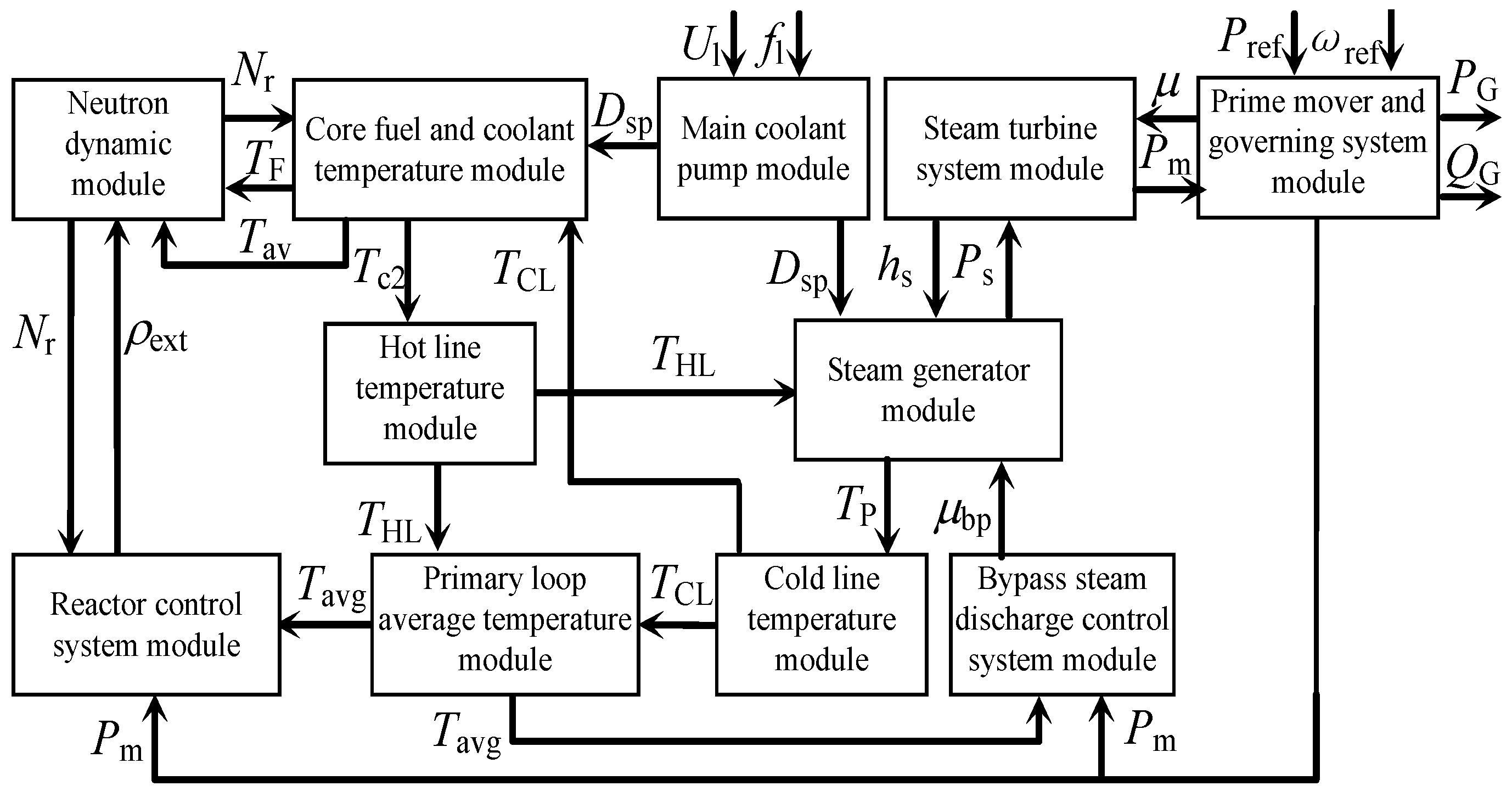
Considering the main equipment, subsystem boundary, operating characteristics and operational parameter testability, the PWR primary loop system model was divided into multiple sub-modules adopting modular modeling method. The established model should fully reflect the energy generation, transmission and transformation process in a NPP. The focus was on the subsystems that had a greater influence on the power plant physical process. The subsystems with lower impact were simplified.

Based on the second-generation PWR nuclear power plant model [9] and the characteristics of the third-generation nuclear power plant, the dynamic AP1000 model of the primary loop system was established for power system simulation. It contains the core neutron dynamic module, the core fuel and coolant temperature module, the hot line and cold line temperature module, the primary loop average temperature module, the steam generator module, the reactor power control system module and the main coolant pump module. Figure 1 shows each sub-module with multi-input multi-output (MIMO) characteristics that are coupled with each other to form an integrated system.

In this figure μ is the tone opening. P_ref and ω_ref are the given unit power and speed, respectively. P_G and Q_G are the generator output active power and reactive power, respectively. h_s is the outlet steam specific enthalpy.

2.1. Reactor and Coolant System Model

Considering the effect of delayed neutrons, the neutron flux density is assumed in the same shape of the spatial distribution at different times. Considering the core and coolant system as a lumped parameter system to simulate normal operation as well as transient processes of the reactor and coolant system, the point reactor kinetics equations of the core neutron dynamic module are as follows:

$$\begin{array}{l}\frac{d{N}_{\mathrm{r}}}{dt}=\frac{{\rho }_{\mathrm{ext}}-\beta }{l}{N}_{\mathrm{r}}+\frac{\beta }{l}{C}_{\mathrm{r}}+({\alpha }_{\mathrm{F}}(T_{\mathrm{F}}-T_{\mathrm{F}0})+{\alpha }_{\mathrm{C}}(T_{\mathrm{av}}-T_{\mathrm{av}0}))N_{\mathrm{r}}\\ \frac{d{C}_{\mathrm{r}}}{dt}=\lambda N_{\mathrm{r}}-\lambda C_{\mathrm{r}}\end{array}$$

(1)

where l is the average neutron lifetime, β is the total share of delayed neutron group and λ is the time delay of equivalent delayed neutron group. C_r is the precursor nuclear density of equivalent single set of delayed neutron. α_F and α_C are the reactivity coefficients of the fuel temperature and coolant temperature, respectively.

Considering the effect of nuclear fission energy on fuel temperature, as well as the heat energy transferred from the fuel to the core coolant, according to energy conservation law and volume balance, the mathematical model of core fuel and coolant temperature module is given by the following expression:

$$\begin{array}{l}\frac{d{T}_{\mathrm{F}}}{dt}=\frac{F_{\mathrm{f}}{P}_0}{{\mu }_f}{N}_{\mathrm{r}}-\frac{\Omega }{{\mu }_f}{T}_{\mathrm{F}}+\frac{\Omega }{2{\mu }_f}{T}_{\mathrm{av}}+\frac{\Omega }{4{\mu }_f}{T}_{\mathrm{HL}}+\frac{\Omega }{4{\mu }_f}{T}_{\mathrm{CL}}\\ \frac{d{T}_{\mathrm{av}}}{dt}=\frac{(1-F_{\mathrm{f}})P_0}{{\mu }_c}{N}_{\mathrm{r}}+\frac{\Omega }{{\mu }_c}{T}_{\mathrm{F}}-\frac{4M+\Omega }{2{\mu }_c}{T}_{\mathrm{av}}+\frac{4M-\Omega }{2{\mu }_c}{T}_{\mathrm{c}1}\\ \frac{d{T}_{\mathrm{c}2}}{dt}=\frac{(1-F_{\mathrm{f}})P_0}{{\mu }_c}{N}_{\mathrm{r}}+\frac{\Omega }{{\mu }_c}{T}_{\mathrm{F}}-\frac{4M+\Omega }{2{\mu }_c}{T}_{\mathrm{av}}+\frac{4M-\Omega }{2{\mu }_c}{T}_{\mathrm{c}2}\end{array}$$

(2)

where T_F0 and T_av0 are the initial temperature values within the fuel and core coolant, respectively. P₀ is the core thermal power. F_f is the heating fuel share. Ω is the heat transfer coefficient between fuel and coolant in the core. μ_f and μ_c are the heat capacities of fuel and core coolant, respectively. M = D_sp × C_pc × m_Cn, in which C_pc is the coolant heat capacity and m_Cn is the rated coolant mass flow.

Ignoring the heat loss of coolant in the pipeline, according to energy conservation law and volume balance, the hot line and cold line temperature module is given by the following equation:

$$\begin{array}{c}\frac{d{T}_{\mathrm{HL}}}{dt}=\frac{1}{{\tau }_{\mathrm{HL}}}(T_{\mathrm{c}2}-T_{\mathrm{HL}})\\ \frac{d{T}_{\mathrm{c}1}}{dt}=\frac{1}{{\tau }_{\mathrm{CL}}}(T_{\mathrm{CL}}-T_{\mathrm{c}1})\end{array}$$

(3)

where τ_HL and τ_CL are the coolant hotline and cold line time constants, respectively. Considering the coolant measuring sensor characteristics, the measured average temperature of the coolant loop circuit can be expressed using first-order inertial link as follows:

$$T_{\mathrm{avg}}=\frac{1}{{\tau }_{\mathrm{c}}s+1}\left(\frac{T_{\mathrm{HL}}+T_{\mathrm{CL}}}{2}\right)$$

(4)

where τ_c is the temperature measuring time constant of coolant.

2.2. Steam Generator Module

The AP1000 NPP uses two Δ125-type U-shaped natural circulation steam generators. Assuming the thermal power from the main pump transmitted to the primary circuit coolant can be neglected, the specific heat of the U-shaped heat transfer tube, the specific heat and density of the coolant are treated as constants. According to mass balance, volume balance and energy conservation law, a steam generator model with centralized parameters containing temperature and pressure equations is established as shown in Equation (5):

$$\begin{array}{l}\frac{\mathrm{d}{T}_{\mathrm{P}}}{\mathrm{d}t}=\frac{2M-{\Omega }_{\mathrm{p}}}{2{\mu }_{\mathrm{p}}}{T}_{\mathrm{HL}}-\frac{2M+{\Omega }_{\mathrm{p}}}{2{\mu }_{\mathrm{p}}}{T}_{\mathrm{P}}+\frac{{\Omega }_{\mathrm{p}}}{{\mu }_{\mathrm{p}}}{T}_{\mathrm{m}}\\ \frac{\mathrm{d}{T}_{\mathrm{CL}}}{\mathrm{d}t}=\frac{2M-{\Omega }_{\mathrm{p}}}{2{\mu }_{\mathrm{p}}}{T}_{\mathrm{HL}}-\frac{2M+{\Omega }_{\mathrm{p}}}{2{\mu }_{\mathrm{p}}}{T}_{\mathrm{P}}+\frac{{\Omega }_{\mathrm{p}}}{{\mu }_{\mathrm{p}}}{T}_{\mathrm{m}}\\ \frac{\mathrm{d}{T}_{\mathrm{m}}}{\mathrm{d}t}=\frac{{\Omega }_{\mathrm{p}}}{4{\mu }_{\mathrm{m}}}{T}_{\mathrm{HL}}+\frac{{\Omega }_{\mathrm{p}}}{2{\mu }_{\mathrm{m}}}{T}_{\mathrm{P}}+\frac{{\Omega }_{\mathrm{p}}}{4{\mu }_{\mathrm{m}}}{T}_{\mathrm{CL}}-\frac{{\Omega }_{\mathrm{p}}+{\Omega }_{\mathrm{S}}}{{\mu }_{\mathrm{m}}}{T}_{\mathrm{m}}+\frac{{\Omega }_{\mathrm{S}}}{{\mu }_{\mathrm{m}}}{K}_{Ps\_Ts}(P_{\mathrm{s}})\\ \frac{\mathrm{d}{P}_{\mathrm{s}}}{\mathrm{d}t}=\frac{{\Omega }_{\mathrm{S}}}{K_{P_{\mathrm{s}}}}{T}_{\mathrm{m}}-\frac{{\Omega }_{\mathrm{S}}}{K_{P_{\mathrm{s}}}}{K}_{Ps\_Ts}(P_{\mathrm{s}})+\frac{Q_{\mathrm{s}}(h_{\mathrm{fw}}-h_{\mathrm{s}})}{K_{P_{\mathrm{s}}}}\end{array}$$

(5)

where T_p is the average temperature of the primary coolant. T_m denotes the U-shaped heat pipe temperature. K_Ps is the steam pressure time constant. K_{Ps_Ts}(P_s) is the conversion relation between the main steam pressure and temperature of the secondary circuit. Ω_p is the heat transfer coefficient between coolant in steam generator and U-shaped heat pipe. Ω_S is the heat transfer coefficient between U-shaped heat pipe and secondary loop steam. μ_p and μ_m are the heat capacities of coolant in the steam generator and U-shaped heat pipe, respectively. h_fw is the inlet temperature specific enthalpy of secondary loop feed water.

2.3. Main Coolant Pump Module

The main coolant pump of the AP1000 is a shielded motor pump, mainly used to complete the circulation of the reactor coolant. The main coolant pump module is established considering the influence of auxiliary power supply voltage and frequency on the main coolant pump speed and flow rate, as shown in Equation (6):

$$\begin{array}{l}{T}_{\mathrm{pj}}\frac{d{\omega }_{\mathrm{p}}^{*}}{dt}=M_{\mathrm{pe}}^{*}-M_{\mathrm{pm}}^{*}\\ M_{\mathrm{pe}}^{*}=k_{\mathrm{e}1}\frac{{U_1^{*}}^2(1-\raisebox{1ex}{${\omega }_{\mathrm{p}}^{*}$}\!\left/ \!\raisebox{-1ex}{$f_{\mathrm{l}}^{*}$}\right.)}{[1+k_{\mathrm{e}2}{f_1^{*}}^2{(1-\raisebox{1ex}{${\omega }_{\mathrm{p}}^{*}$}\!\left/ \!\raisebox{-1ex}{$f_{\mathrm{l}}^{*}$}\right.)}^2]f_{\mathrm{l}}^{*}}\\ M_{\mathrm{pm}}^{*}={{\omega }_{\mathrm{p}}^{*}}^2\\ D_{\mathrm{sp}}^{*}={\omega }_{\mathrm{p}}^{*}/{\omega }_{\mathrm{pr}}^{*}\end{array}$$

(6)

where T_pj is the inertia time constant of main coolant pump rotor. $M_{\mathrm{pe}}^{*}$ and $M_{\mathrm{pm}}^{*}$ are the electromagnetic torque and resistance moment per-unit values, respectively. k_e1 and k_e2 are the characteristic coefficients of the asynchronous motor. ${\omega }_{\mathrm{p}}^{*}$ and ${\omega }_{\mathrm{pr}}^{*}$ are the speed and rated speed per-unit values of the asynchronous motor, respectively; $f_1^{*}$ is the auxiliary power bus frequency per-unit value; $U_1^{*}$ is the auxiliary power bus voltage per-unit value and $D_{\mathrm{sp}}^{*}$ is the main coolant pump flow per-unit value.

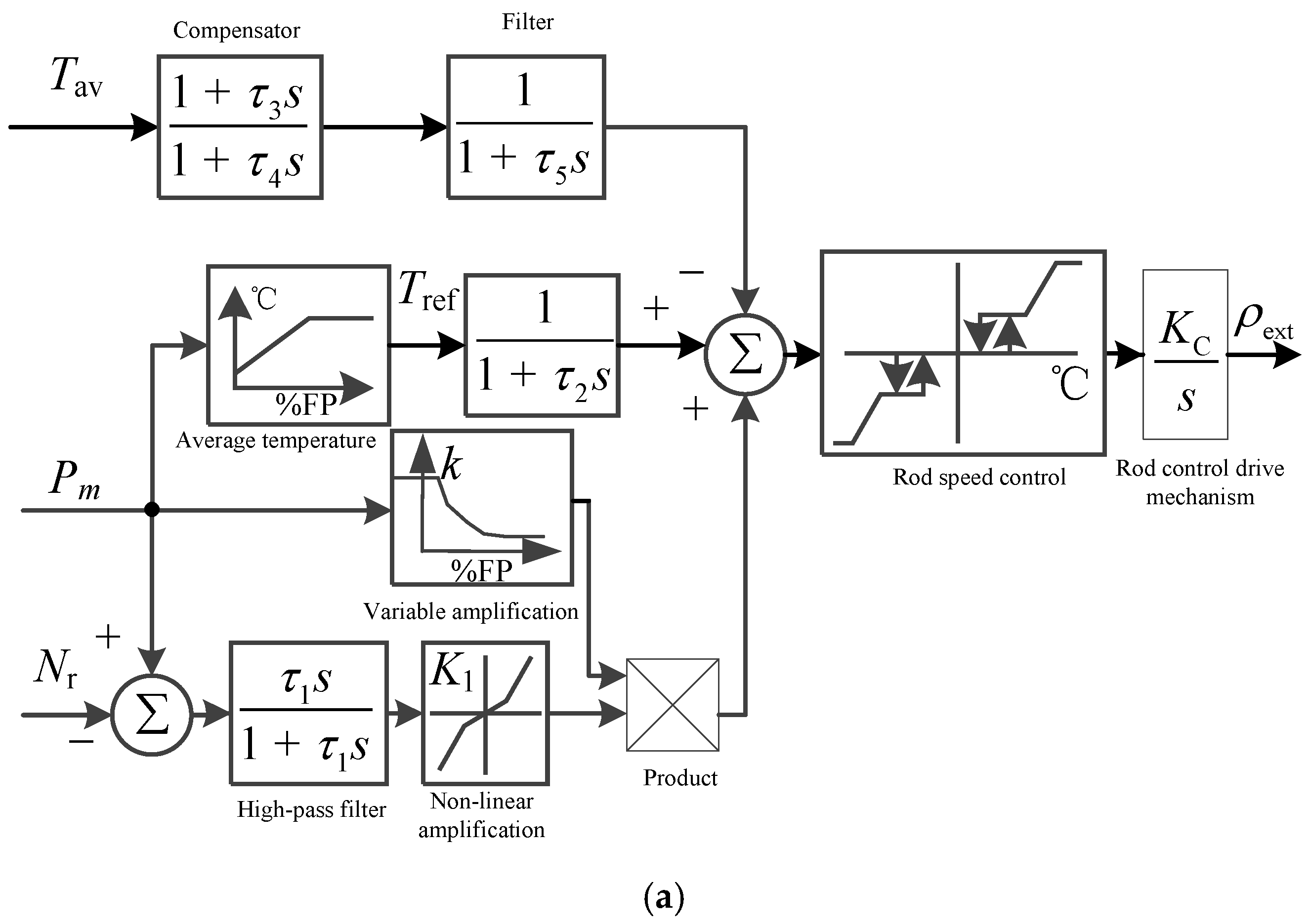
2.4. Reactor Power Control Module

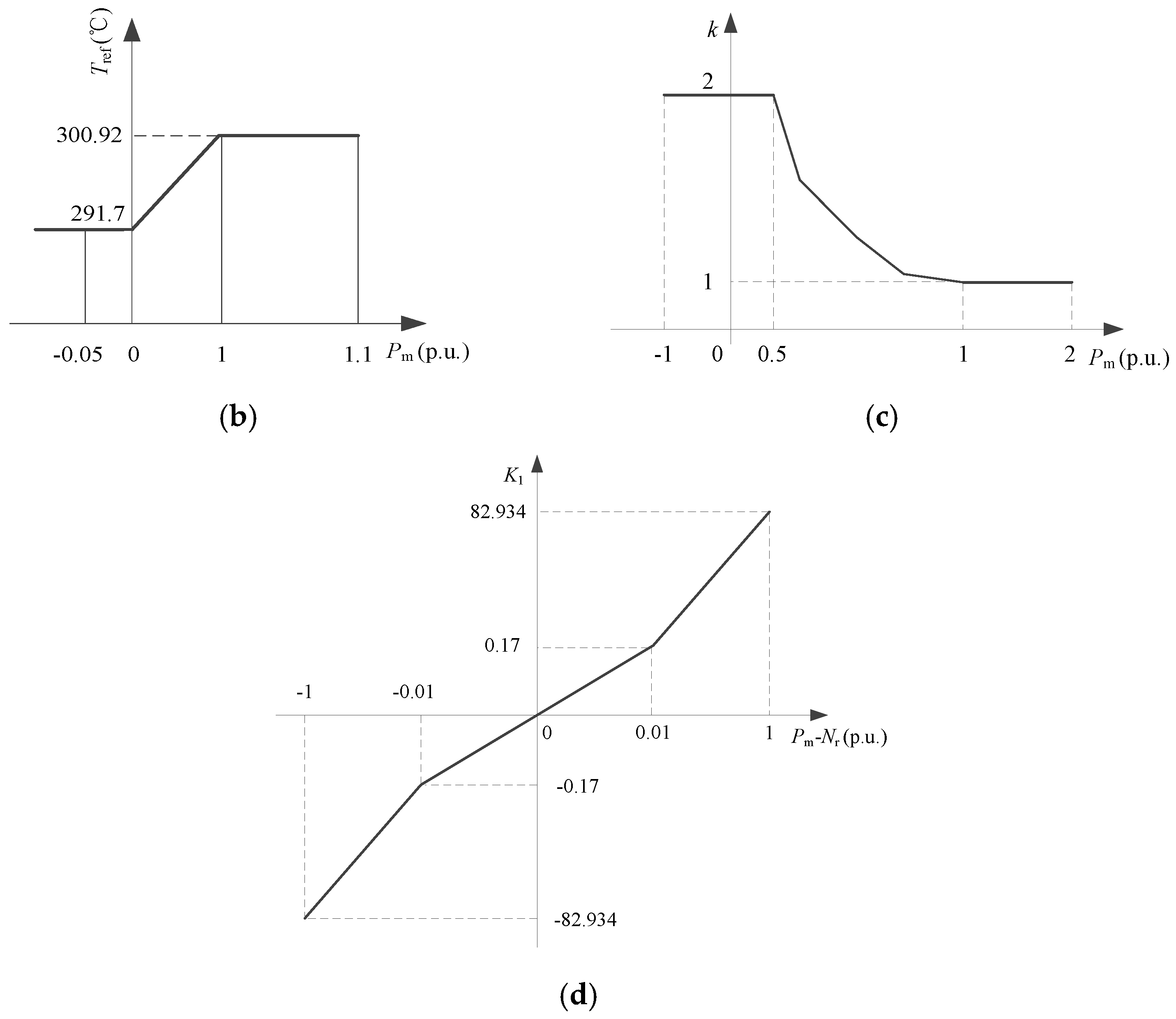
The PWR reactor power control module adjusts the reactor neutron flux density which reflects the core power by removing or inserting rods. The dead zone and hysteresis links are applied to maintain the average primary coolant temperature in the designed control band. Figure 2 showed the third-generation reactor power control system module including the average temperature link, the variable amplification link, the nonlinear amplification link, the rod speed control link, the compensator and filter link. The variable measurement links were omitted. The rod speed varies over the range of 8–72 steps per minute depending on the input signal level.

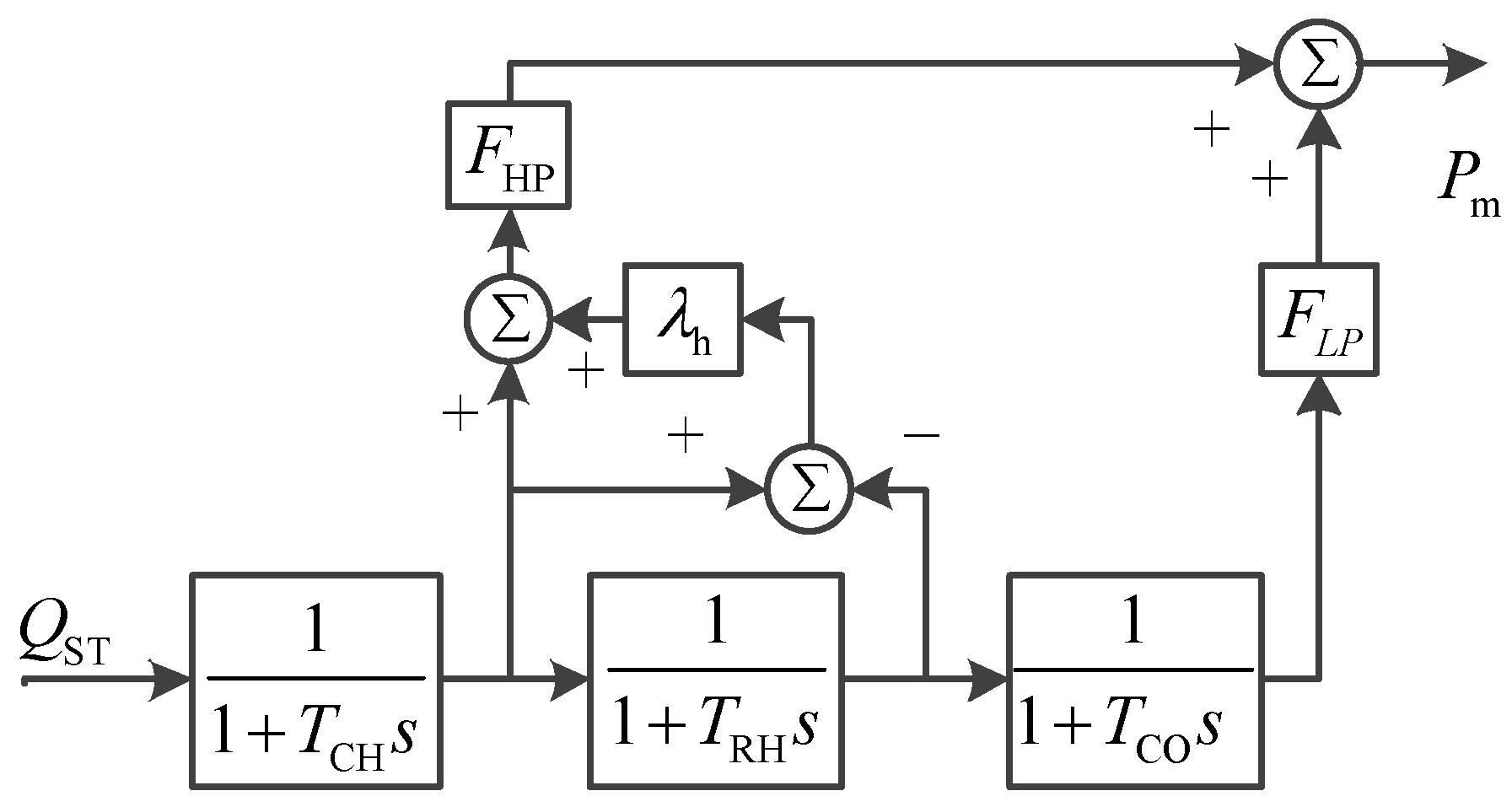
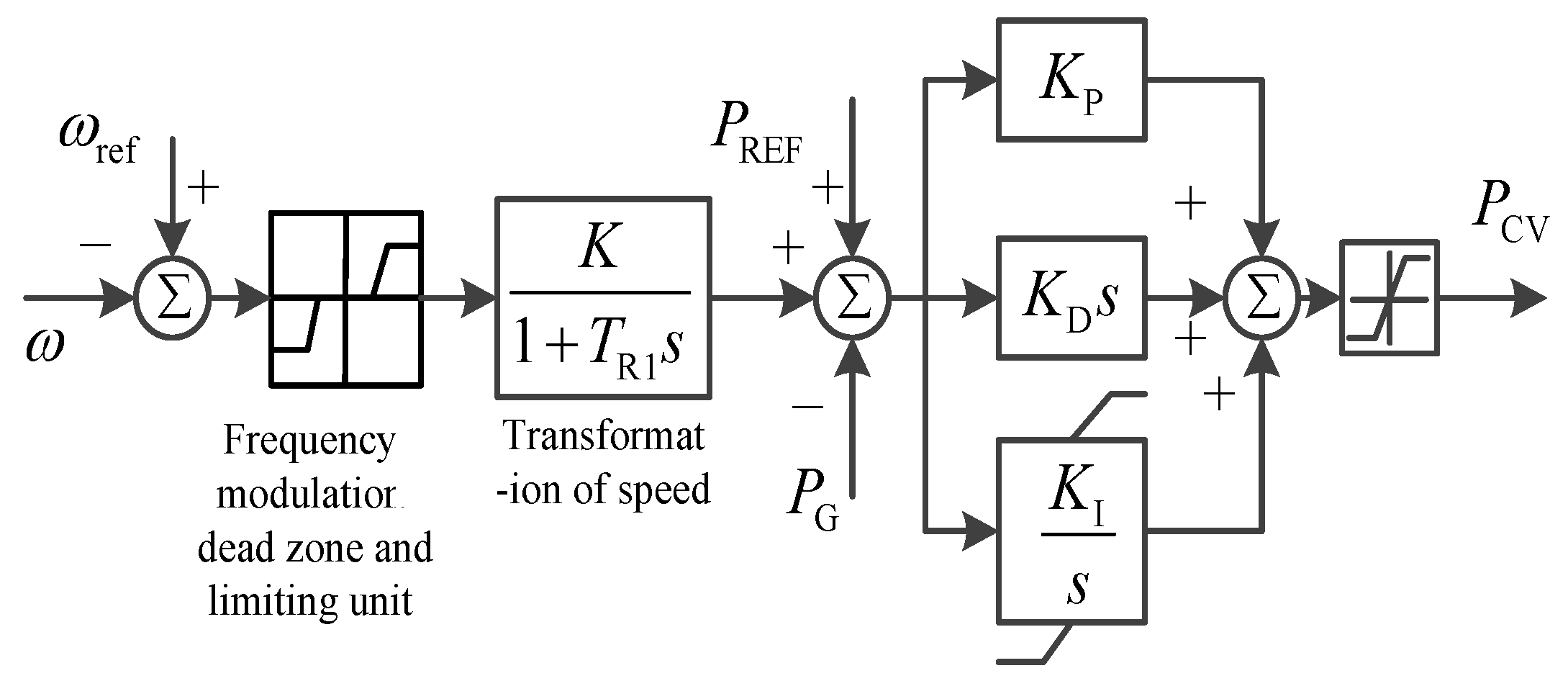
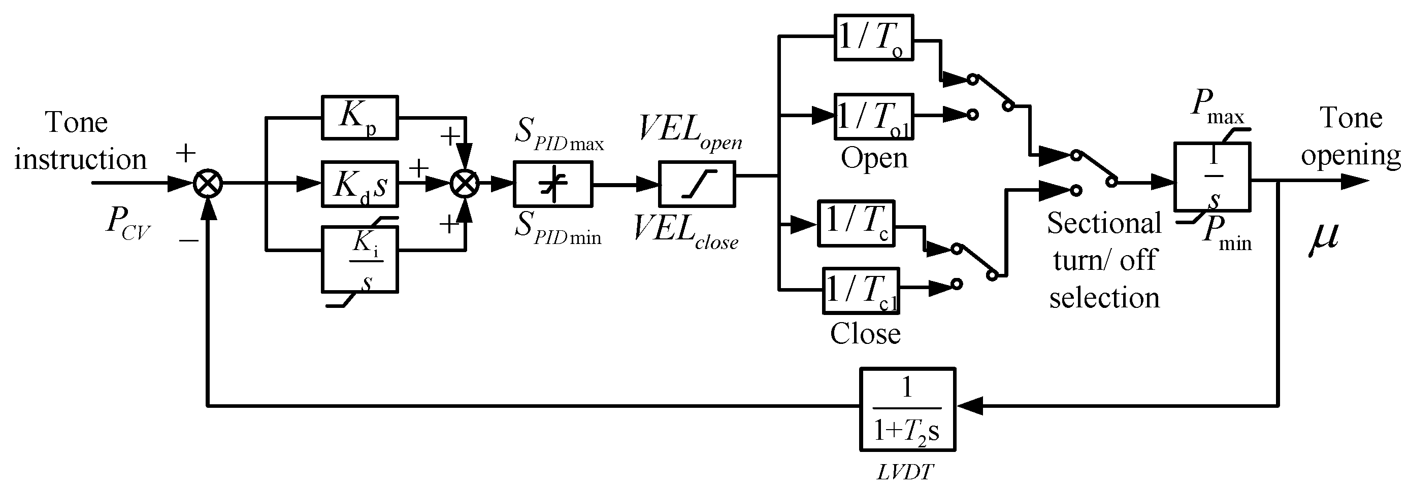
2.5. Steam Turbine and Its Control System Module

The steam turbine of the AP1000 has characteristics of a single-shaft with four-cylinder (i.e., a high-pressure cylinder and three low-pressure cylinders) reheat condensing steam turbine at half speed. A digital electric-hydraulic governor is used to respond to the frequency and power changes. The steam turbine module, speed control system module (i.e., the governor and electro-hydraulic servo system) and turbine bypass control system module suitable for the AP1000 are shown in Figure 3, Figure 4, Figure 5 and Figure 6, respectively, in which the main turbine steam flow is shown as follows:

$$Q_{\mathrm{ST}}=\mu \cdot P_{\mathrm{s}}/P_{\mathrm{sn}}$$

(7)

where P_sn is the rated main steam pressure.

In Figure 5, K_p, K_i and K_d are the proportional, integral and differential coefficients, respectively. S_PIDmax and S_PIDmin are the upper and low limits, respectively. VEL_open and VEL_close are the rapid opening and rapid closing coefficients, respectively. T₂ is the time constant of oil motive stroke feedback link, usually taken as 0.02 s. T_o and T_c are defined as the main on/off time constants while T_o1 and T_c1 are defined as the auxiliary oil motive on/off time constants. The segmented opening and closing tone values are determined according to actual conditions.

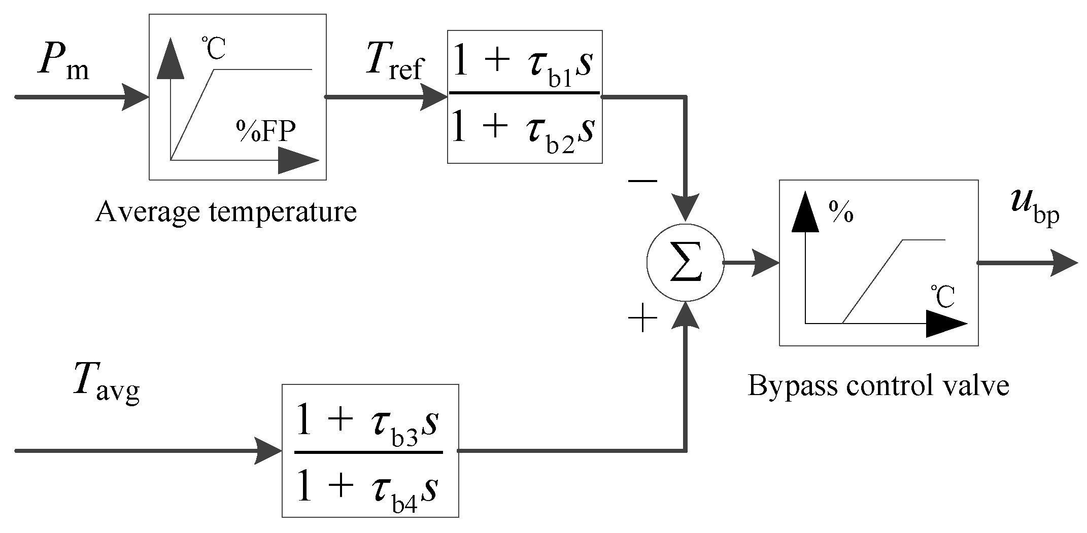
Figure 6 shows the steam turbine bypass control system diagram in the case that a large deviation between the turbine mechanical output power and the coolant average temperature equivalent to the core power appeared. The steam was discharged through the bypass valve to ensure reactor safety. τ_b1, τ_b2, τ_b3 and τ_b4 are compensator and filter time constants. The %FP symbol in Figure 6 means the percentage of the rated full power.

2.6. Generator Mathematical Model

As the large-scale nuclear power plant uses a half-speed steam turbine generator unit, the PARK equation is adopted to establish the mathematical model of the six windings synchronous generator. The voltage and flux equations are shown in Equations (8) and (9):

$$\mathit{u}=p\mathit{\Psi }+\mathit{\omega }\mathit{\Psi }+\mathit{r}\mathit{i}$$

(8)

$$\mathit{\Psi }=\mathit{x}\mathit{i}$$

(9)

where u = [u_d, u_q, u_f, 0, 0, 0]^T, Ψ = [Ψ_d, Ψ_q, Ψ_f, Ψ_D, Ψ_g, Ψ_Q]^T, i = [i_d, i_q, i_f, i_D, i_g, i_Q]^T, r = diag{R_s, R_s, R_f, R_D, R_g, R_Q}, $\mathit{\omega }=\left[\begin{array}{cccccc}0& -{\omega }_{\mathrm{r}}& 0& 0& 0& 0\\ {\omega }_{\mathrm{r}}& 0& 0& 0& 0& 0\end{array}\right]$. x is a reactance matrix of size 6 × 6.

The motion equations of the generator rotor are shown in Equations (10) and (11):

$$T_{\mathrm{j}}\frac{\mathrm{d}\omega }{\mathrm{d}t}=T_{\mathrm{m}}-T_{\mathrm{e}}-D_{\omega }(\omega -{\omega }_0)$$

(10)

$$\frac{\mathrm{d}\delta }{\mathrm{d}t}=\omega -{\omega }_0$$

(11)

where T_j is the inertial time constant of generator. D_ω is the damping coefficient. T_m is the mechanical torque. T_e = Ψ_d × i_q – Ψ_q × i_d, δ is the power angle and ω₀ is the rated speed (i.e., ω₀ = 1).

The model parameters were obtained according to the AP1000 design manual, the test curves of second-generation operating PWR units and through comparison with the simulation curves from the PCTRAN software.

3. Parameter Identification Method and Process

3.1. Particle Swarm Optimization Algorithm Based on Random Perturbation

The PSO algorithm is a bionic algorithm used to solve optimization problems. D is the parameter dimension. The position of the i-th particle is described as $x_i=(x_{i1},x_{i2},\cdots ,x_{iD})$. The velocity of the i-th particle is described as $v_i=(v_{i1},v_{i2},\cdots ,v_{iD}),1\le i\le m$. The historical best point experienced by the i-th particle is denoted as $p_i=(p_{i1},p_{i2},\cdots ,p_{iD})$. The best point for all particles is denoted as $p_g=(p_{g1},p_{g2},\cdots ,p_{gD})$. The position and velocity of the particles needed to be constantly updated by the following equation:

$$\begin{array}{l}{v}_{iD}^{k+1}=v_{iD}^k+C_1\times \xi \times (p_{iD}^k-x_{iD}^k)+C_2\times \eta \times (p_{gD}^k-x_{iD}^k)\\ x_{iD}^{k+1}=x_{iD}^k+v_{iD}^{k+1}\end{array}$$

(12)

where C₁ and C₂ are learning factors. ξ and η are uniformly distributed random numbers in [0,1]. k reflects the k-th number of iterations.

The concept of inertia weight was introduced in the particle’s velocity updating equation to adopt global search followed by local search for solution efficiency [11]. The position and velocity were written as the following:

$$\begin{array}{l}{v}_{iD}^{k+1}=\omega \times v_{iD}^k+C_1\times \xi \times (p_{iD}^k-x_{iD}^k)+C_2\times \eta \times (p_{gD}^k-x_{iD}^k),V_{\min }\le v_{iD}^{k+1}\le V_{\max }\\ \omega ={\omega }_{\max }-({\omega }_{\max }-{\omega }_{\min })\times k/MI,1\le k\le MI\end{array}$$

(13)

where ω is the inertia weight. V_min and V_max are the minimum and maximum velocity values. MI is the largest iteration.

Let C₁ and C₂ change linearly and the convergence factor is introduced by the following expression:

$$\begin{array}{l}{C}_1=C_{1\max }-(C_{1\max }-C_{1\min })\times k/MI\\ C_2=C_{2\max }-(C_{2\max }-C_{2\min })\times k/MI\\ x_{iD}^{k+1}=x_{iD}^k+\lambda \times v_{iD}^{k+1}\end{array}$$

(14)

where λ is the convergence factor. The velocity and position of the particles cannot exceed their upper and lower limits.

To further enhance the optimization ability, the particle initial population was generated by chaos method to achieve better initial solution. The two-dimensional cat map was written as follows:

$$\{\begin{array}{l}{x}_{iD}^{k+1}=\mathrm{mod}(x_{iD}^k+v_{iD}^k,1)\\ v_{iD}^{k+1}=\mathrm{mod}(x_{iD}^k+2v_{iD}^k,1)\end{array}$$

(15)

where “mod” means modular operation.

Furthermore, the random perturbation method was introduced to avoid the parameters staying at the boundary value of the given parameter scope and get the appropriate solution. The global optimal value of the parameter was perturbed as follows:

$${\mathrm{z}}_{\mathrm{besti}}={\mathrm{z}}_{\mathrm{besti}}\times (1+K\times \mathrm{randn})i\in [1,D]$$

(16)

where z_besti is a certain identified parameter and “randn” stands for the standard normal distribution function. The formula “z_besti × K × randn” reflects the perturbation value, which can make z_besti larger or smaller, wherein K is the perturbation coefficient which is set reasonably according to the order of magnitude of the parameter. Various parameters were chosen to be perturbed. The number of perturbed parameters were reduced gradually during solving process to make the solution stabilized finally.

The fitness function of the algorithm was expressed as follows:

$$f=\frac{{\displaystyle \sum _{j=1}^N{\displaystyle \sum _{i=1}^T(y_j(i)}-y_{j0}(i){)}^2}}{T},1\le n\le N$$

(17)

where T is the total data points. n and N are the selected number of model output variables for identification and the total output variable number, respectively. y_j(i) and y_j0(i) are the simulation and test results of the i-th data point for the j-th output variable, respectively. The random perturbation may not reduce the fitness function sometimes, but it increases the parameter difference which is helpful for global parameter optimization.

3.2. Parameter Identification Process

Both the single input variable steps and multiple input variable steps were given to get the test data under various working conditions, which was useful for the actual test work as well as for parameter identification. The more working conditions and more output variables that were used in one identification process instance, the more difficult the identification was. The variable and parameter constraints were explored according to the design characteristics and the parameter effect on the model gain. The noise reduction using wavelet de-noising and data smoothing were applied to reduce the effect of noise to test signals. The data resampling was used to get the appropriate data points for identification. The model parameters are obtained in the following steps.

Step 1:

Divide the PWR primary loop system model into several modules properly.

Step 2:

Select the input and output variables of tested data for identification of each module.

Step 3:

Have preprocessing of noise reduction, data resampling and data normalization to a range of 0 to 1 for some variables (e.g., N_r, D_sp and so on) before parameter identification.

Step 4:

Make the model initially stable through variable initialization based on the differential equations of each module and program setting method.

Step 5:

After obtaining the constraints of variables and parameters, calculate some parameters according to the operating characteristics for PWR primary loop system. Identify parameters of each module using the RP-PSO algorithm.

Step 6:

Conduct sensitivity analysis for model parameters. Check parameters under various conditions based on sub-module and the integrated model.

Figure 7a shows the nuclear power parameter identification process diagram. Figure 7b shows the parameter identification process diagram with the RP-PSO and Simulink. Big sensitivity is beneficial for parameter identification in both time domain and frequency domain analysis. Apart from parameter influence analysis on model dynamic simulation, the trajectory sensitivity analysis [25] could provide a reference for parameter identifiability and reference for the perturbed parameter selection in the RP-PSO algorithm (see Figure 7a).

4. Model Parameter Identification and Validation

The tested data was obtained from a sub-module test, or the integrated model test. It required more than 300 s for the steam generator module. The main features of the PWR primary loop system model parameter identification were analyzed through the specific identification of each module. It is important to keep the model initially stable before parameter identification.

4.1. Model Initialization Based on Differential Equations and Program Setting

The rod position control is an integral part of the AP1000. When the input variable deviation is not within the dead band, there will be a rod position output, which works on another module. As a result, more variables are changed. The model initialization is needed to make the model initially stable, which is also conducive to the parameter identification work.

For the mathematical differential equations of each module given in Section 2, let the derivative of the variables in the left sides of the equations equal zero. Then, the initial variable values can be calculated under a certain stable condition by the following expression:

$$\begin{array}{l}{C}_{\mathrm{r}0}=\frac{N_{\mathrm{r}0}\beta }{l\lambda }\\ T_{\mathrm{av}0}=\frac{\Omega \times (T_{\mathrm{c}20}-T_{\mathrm{c}10})}{8\times M}+0.5\times (T_{\mathrm{c}10}+T_{\mathrm{c}20})\\ T_{\mathrm{F}0}=\frac{{\mathrm{F}}_{\mathrm{f}}\times {\mathrm{P}}_0\times N_{\mathrm{r}0}}{\Omega }+0.25\times (T_{\mathrm{c}10}+T_{\mathrm{c}20})+0.5\times T_{\mathrm{av}0}\\ T_{\mathrm{m}0}=T_{\mathrm{s}0}+\frac{M\times \left(T_{\mathrm{HL}0}-T_{\mathrm{CL}0}\right)}{2\times {\Omega }_{\mathrm{s}}}\\ T_{\mathrm{p}0}=T_{\mathrm{m}0}\times 2-T_{\mathrm{av}0}+\frac{M\times \left(T_{\mathrm{HL}0}-T_{\mathrm{CL}0}\right)}{{\Omega }_{\mathrm{p}}}\end{array}$$

(18)

where N_r0 refers to a certain core power. It should be noted that C_r, which is useful for identification analysis, is an intermediate variable whose value is difficult to be obtained. The initial variable values are closely related to the design parameters such as Ω, Ω_s and Ω_p.

The initial values of some temperature variables set by the program were written as follows:

$$\begin{array}{l}{T}_{CL0}=280.7-\left(P_{\mathrm{m}0}-1\right)\times 11\\ T_{HL0}=321.1+\left(P_{\mathrm{m}0}-1\right)\times 29.4\\ T_{\mathrm{s}0}=271.3-\left(P_{\mathrm{m}0}-1\right)\times \left(291.7-271.3\right)\end{array}$$

(19)

where P_m0 is the given mechanical power value.

4.2. Parameter Identification Analysis

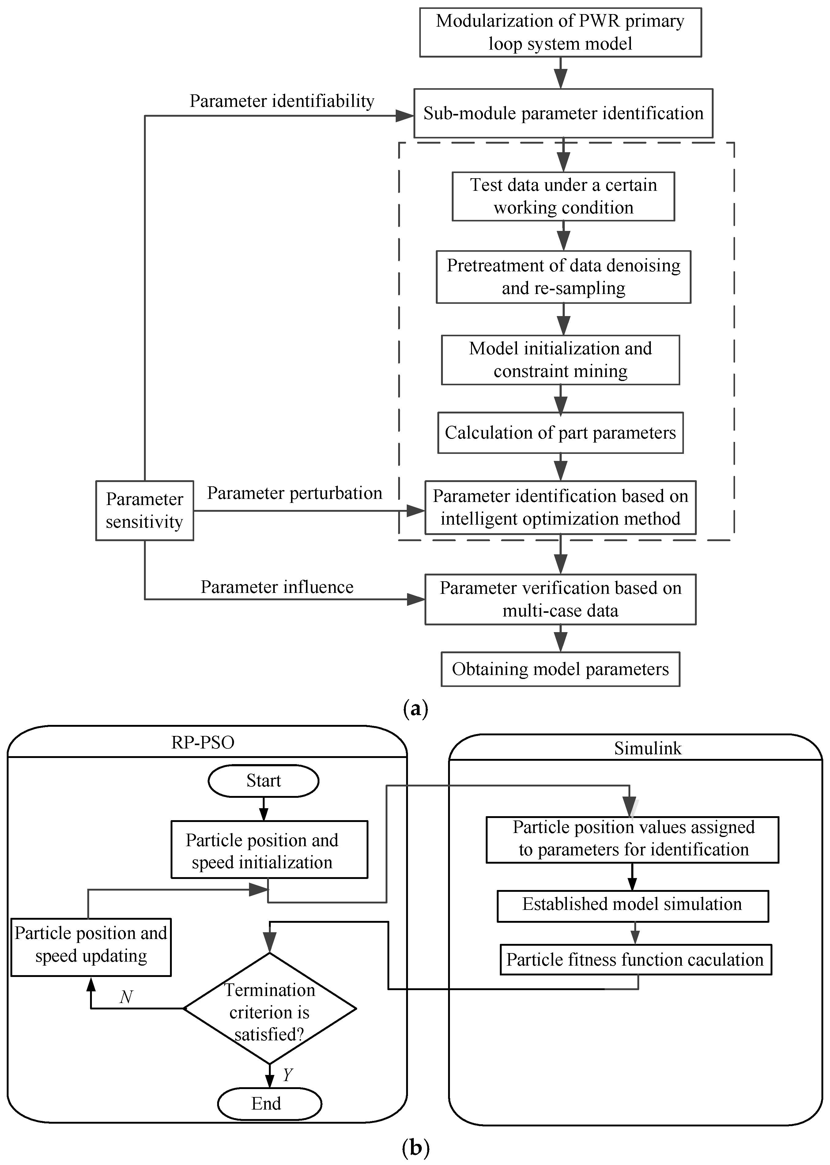
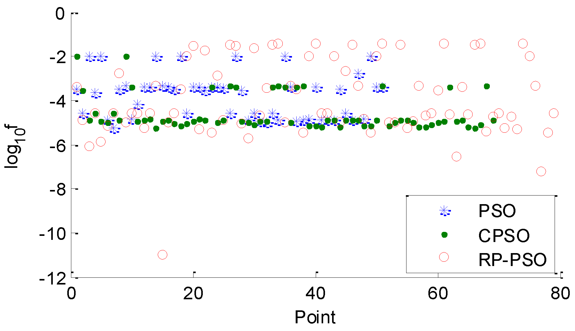
The model parameters were identified by the RP-PSO algorithm with the parameter identification process given in Section 3.2. The parameters for the RP-PSO algorithm were set as ω_max = 0.7, ω_min = 0.01, C_1max = 2.5, C_1min = 0.5, C_2max = 2.5, C_2min = 0.5, V_max = 1, V_min = −1, MI = 200. The population and iteration in the algorithm was set as 200. The largest iteration of 200 was the algorithm termination criterion. A large parameter range was given for the sake of objectivity. The parameter scope was given with a range of 0–1 for the parameters of the core neutron dynamic module, or there was a scope of 0–500 for the other parameters. When the parameter value exceeded 500, the parameter upper limit was set to a 2 order of magnitude larger than its actual value.

Next, it is important to get the model simulation curves under certain working conditions as tested curves with given appropriate parameter values. The data sampling frequency was 0.01 s per point. If the identified parameters were the same with the given values, the fitness function value of the algorithm should be infinitely close to zero.

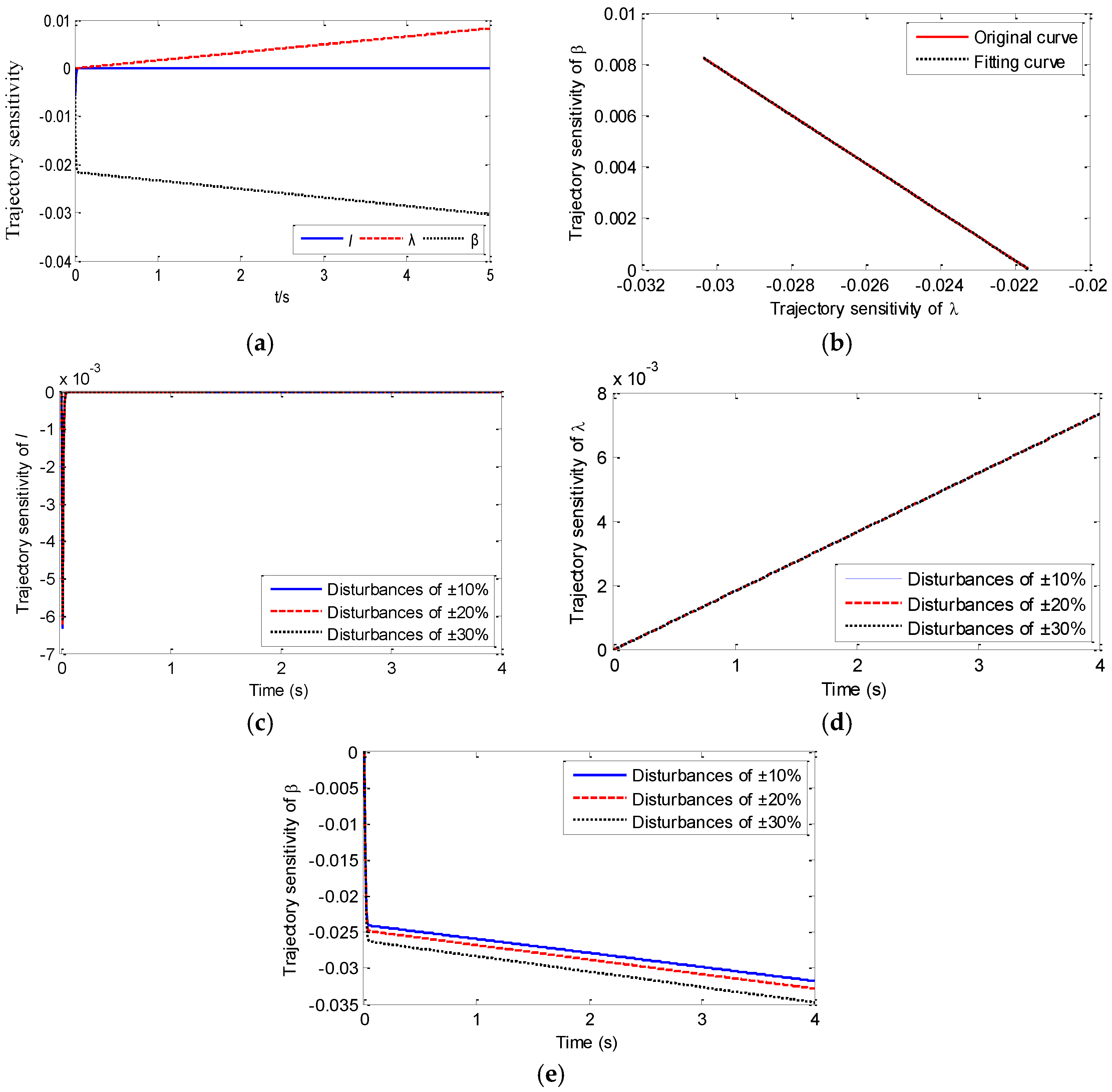
4.2.1. Core Neutron Dynamic Module Parameter Identification

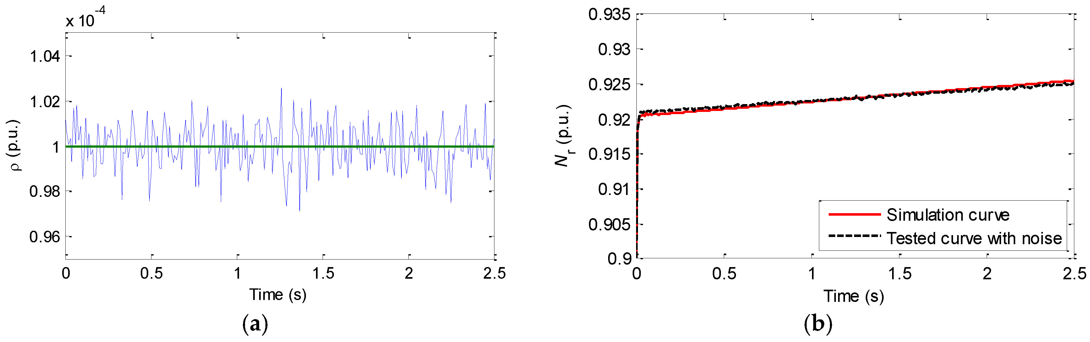
Regardless of the temperature feedback, ρ and N_r are the input and output variables of the core neutron dynamic module, respectively. Supposing a step change of ρ from 0 to 0.0001 p.u. (i.e., per unit) at 1 s, the deviation of N_r was selected as the fitness function to identify l, λ and β.

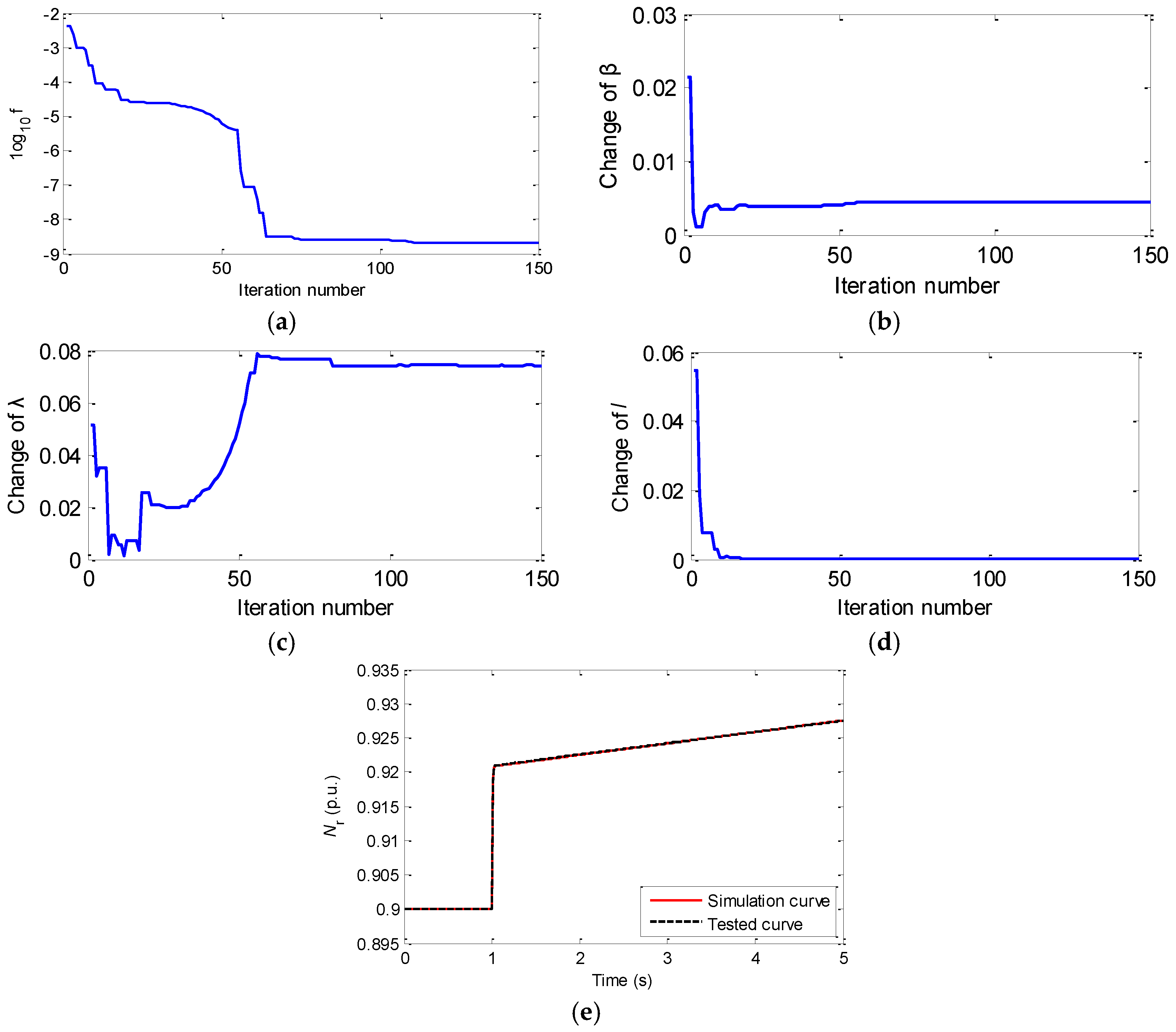
Figure 8 shows the simulation comparison. The identified parameter values changed with iteration increase until they reached their true values after 80 iterations. The fitness function value reached a negative 9 order of magnitude with the identified parameter values in full compliance with their actual values. The simulation curve was consistent with the tested curve as N_r changed from the initial value of 0.9 p.u. (i.e., per unit) with a suddenly steep change to about 0.92 in about 0.03 s, followed by a slower linear growth (see Figure 8e).

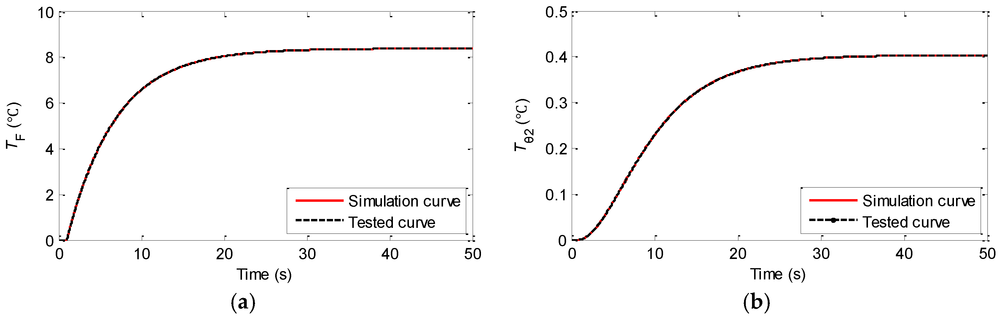
4.2.2. Core Fuel and Coolant Temperature Module Parameter Identification

N_r and T_θ1 are the input variables. T_F, T_θ2 and T_av are the output variables. Given a step change of N_r from 0 to 0.01 at 1 s with all the initial variable values of 0, the parameters identified were fit with their real values as the fitness function value reached negative a 11 order of magnitude. Figure 9 showed the simulation results, proving the effectiveness of the parameter identification. Each output variable raised to a steady-state value with no overshoot.

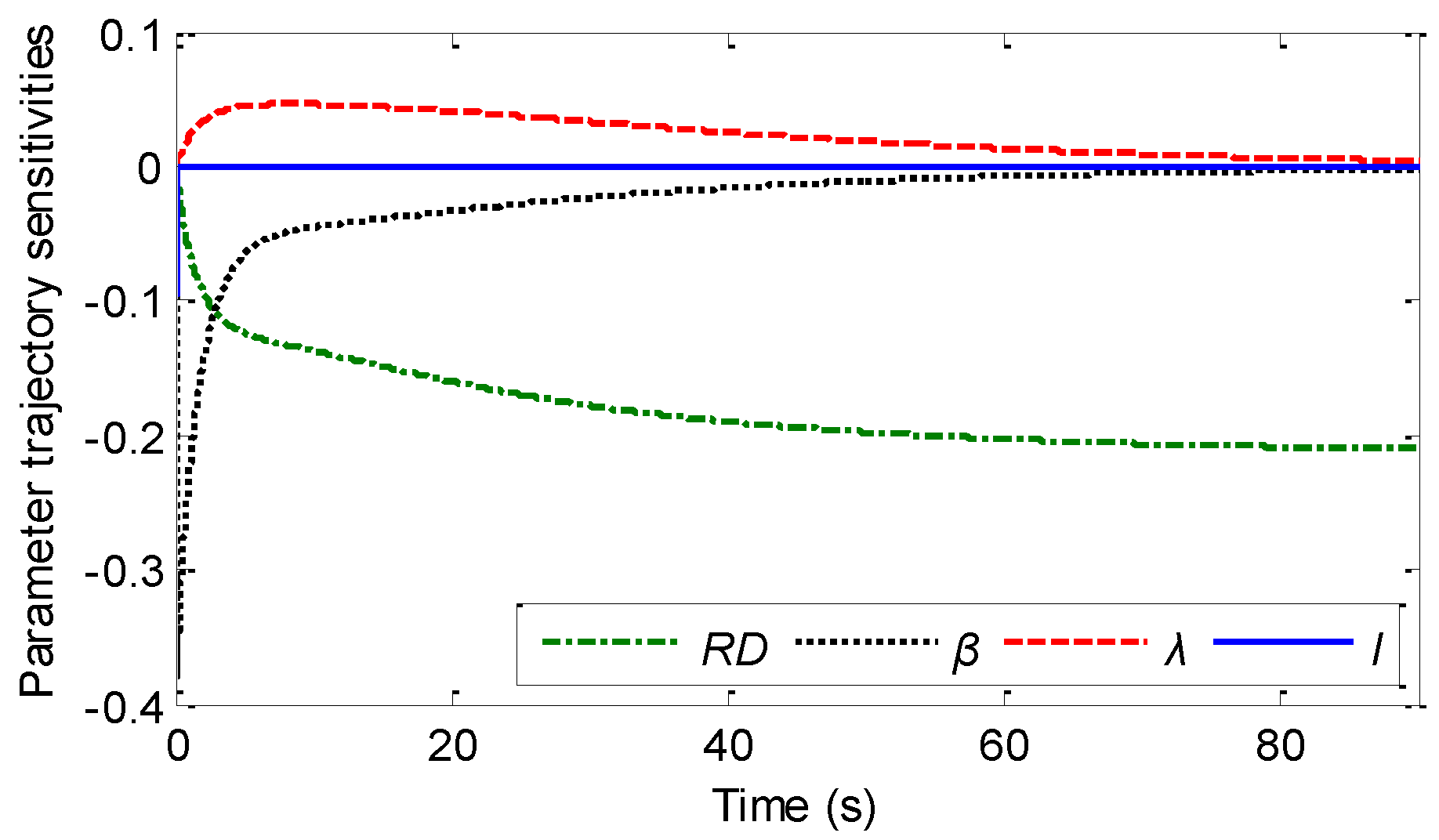
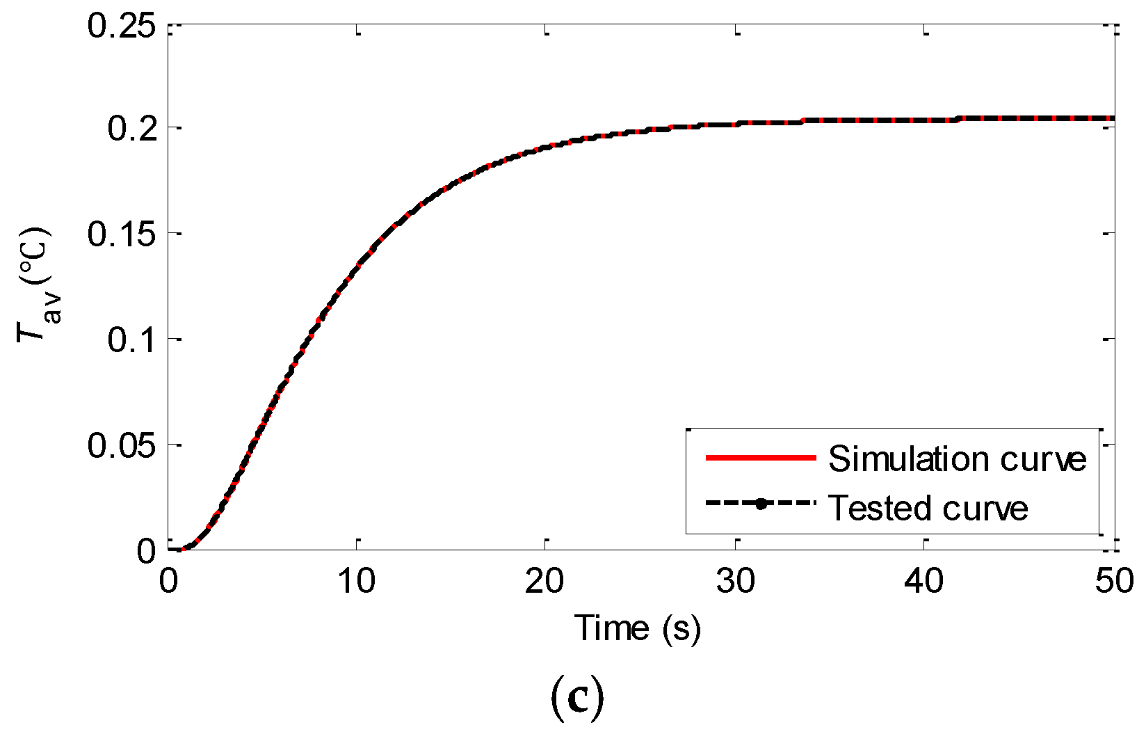
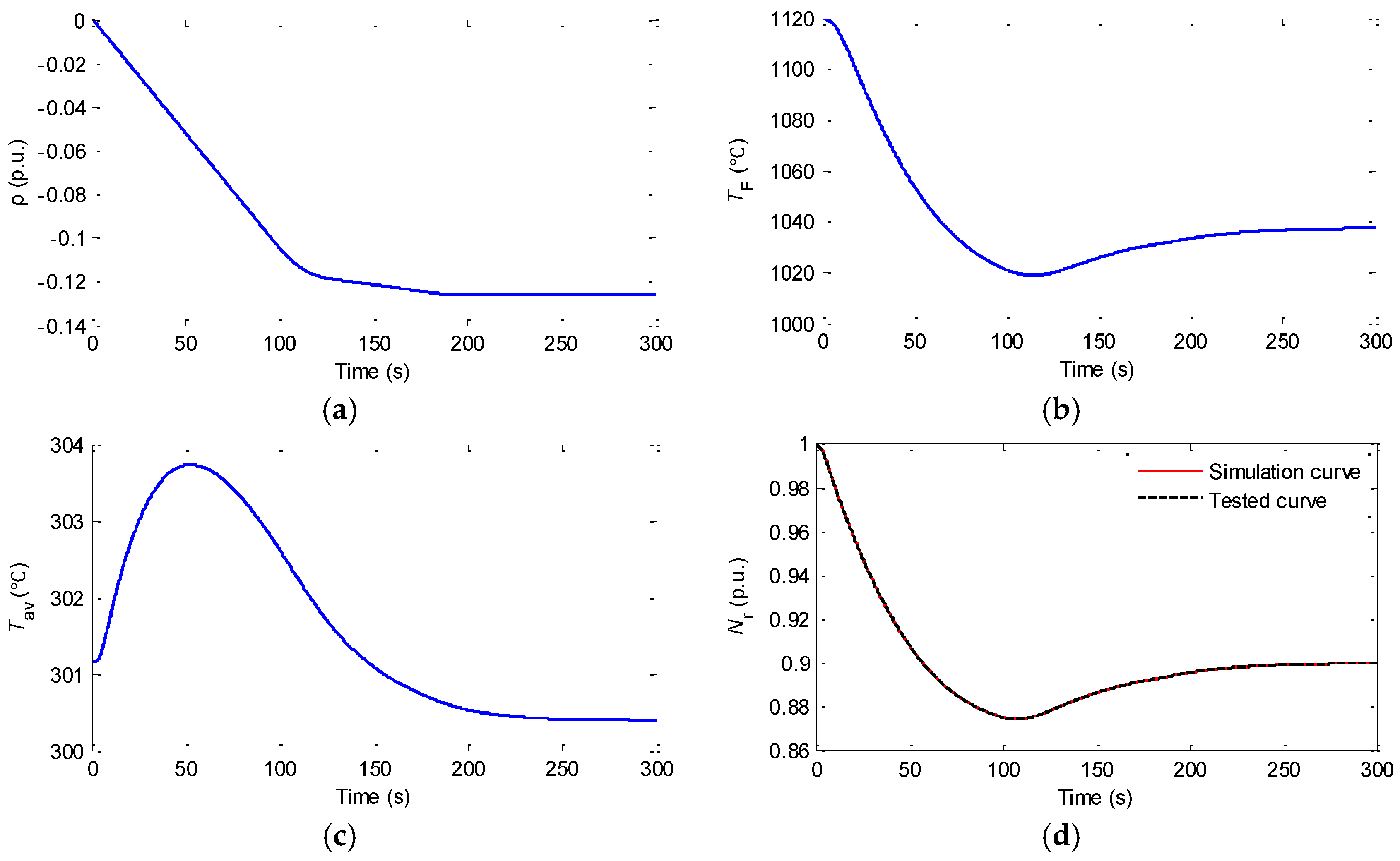
4.2.3. Reactor Power Control System Module Parameter Identification

The input variables are T_avg, and, P_m and N_r. ρ_T is the output variable. Since the transfer function $\frac{1+{\tau }_{3}s}{1+{\tau }_{4}s}$ was the lead link, τ₃ was larger than τ₄.

For the reactor power control system module, the tested data were obtained under a nuclear power change from the rated power of 1–0.9 based on the whole PWR primary loop system model. Furthermore, the turbine bypass control system module was omitted due to its smaller effect when the power changed to 0.1. As the fitness function value reached a negative 14 order of magnitude, the parameters identified were almost the same as their actual values. Figure 10 showed the simulation result after identification. ρ_T declined approximately linearly from 0 before 110 s, followed by a slower decline, until eventually it reached a steady level. The simulation curve fitted the tested curve well.

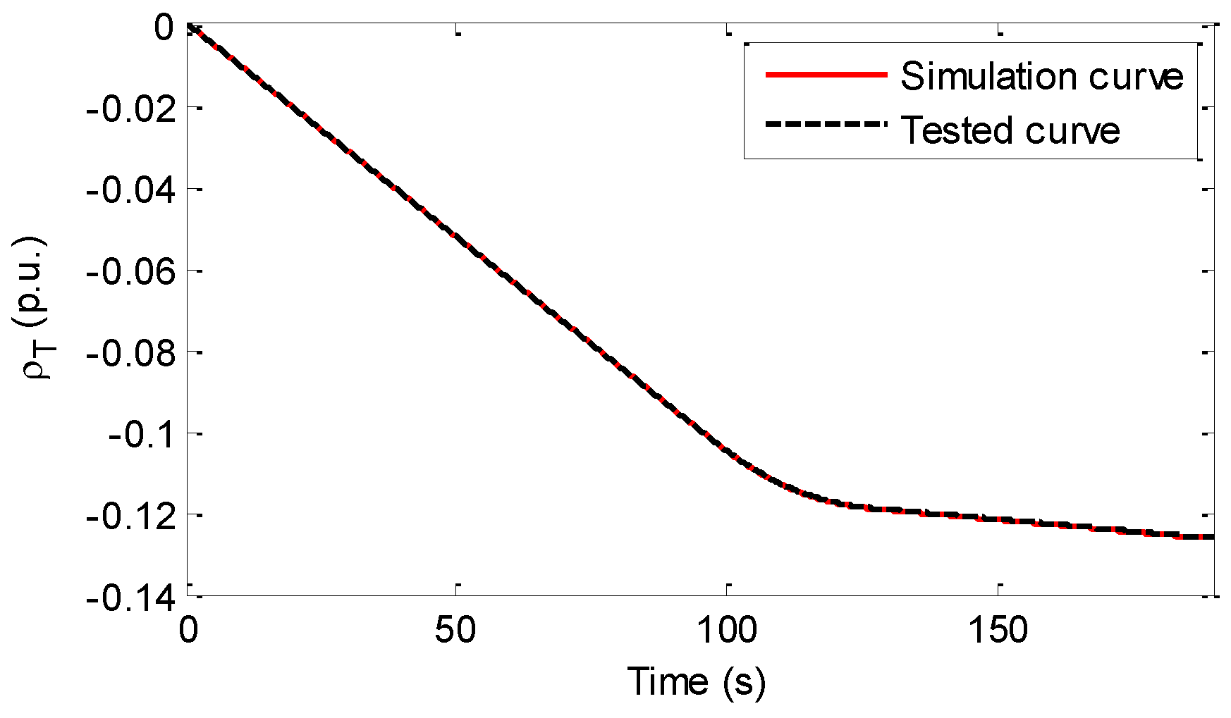
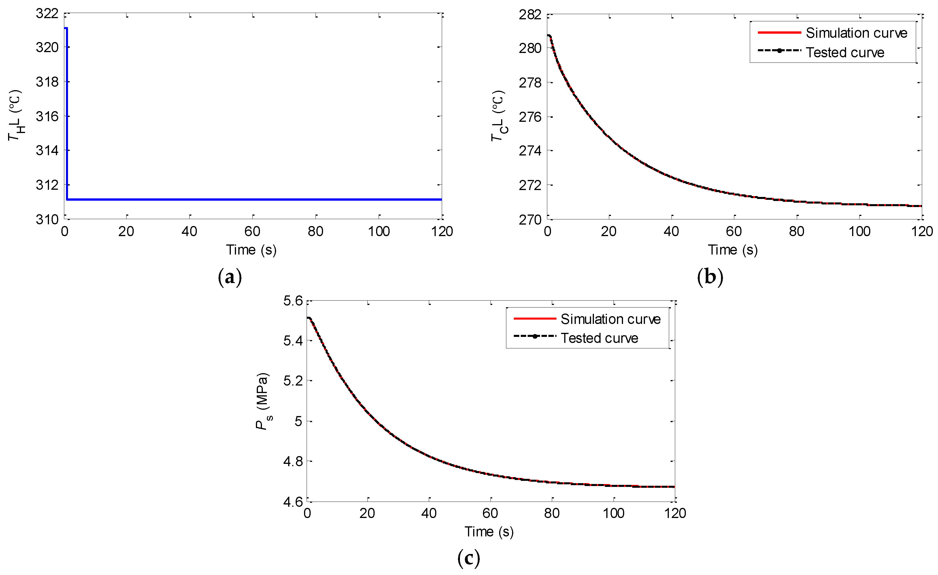
4.2.4. Steam Generator Module Parameter Identification

The input variables are T_HL and Q_sg. Besides some other intermediate variables, T_CL and P_s are the main output variables. The steam generator parameters are mainly related to design parameters with different order magnitudes large to a 7 order of magnitude. Supposing that Q_sg was constant at 1, it gave T_HL a step change of 10 °C from the rated value of 321.1 °C at 1 s. Both the simulation and tested deviation values of T_CL and P_s were used in the fitness function. Figure 8 shows the input T_HL change and output variable simulation comparison.

The simulation result could basically fit with the tested curve (see Figure 11). The variable curves of another condition with Q_sg that were given a step change from 1 to 0.9 were more complex. The identification result using single variable deviation (i.e., the deviation of T_CL or P_s) as the fitness function could not match multiple output variable curves. Thus, the identified parameters might only fit several output variables or parts of the tested curves, if the output variables and tested curves chosen for identification are unable to completely reflect the variable transition process.

Moreover, the parameters of the turbine bypass control system module and the time constants of the cold line, hot line and primary loop average temperature module were easy to be identified, which were omitted in details due to space limitations. Besides the designed parameters,

Table 1. Sub-module parameters.

Core neutron dynamic module	l	Average neutron lifetime
	β	Total share of delayed neutron group
	λ	Time delay of equivalent delayed neutron group
	αF	Reactivity coefficient of fuel temperature
	αC	Reactivity coefficient of coolant temperature
Reactor control system module	KC	Position coefficient of control rods
	τ1, τ2, τ3, τ4 and τ5	Time constants of compensator and filter
Cold line, hot line and primary loop average temperature module	τHL and τCL	Hot and cold line time constants
	τc	Temperature sensor time constant
Core fuel and coolant temperature module	a1 = P0 × Ff/μf, a2 = P0 × (1 − Ff)/μc, a3 = Ω/μf, a4 = Ω/μc, a5 = M/μc
Steam generator module	KPs	Steam pressure time constant
	KPs_Ts	Conversion coefficient between pressure and temperature of the secondary loop main steam
	c1 = M/μp, c2 = Ωp/μp, c3 = Ωp/μm, c4 = ΩS/μm, c5 = ΩS, c6 = (hs − hfw) × Gsn

lists the main sub-module parameters.

Table 2. Model parameter values.

Parameter	Value	Identified	Relative Error	Parameter	Value	Identified	Relative Error
l	2.1 × 10−5 s	1.99 × 10−5 s	5.238%	τ2	56.3514 s	56.1513 s	0.355%
β	4.4 × 10−3	0.004417	0.386%	τ3	12.1755 s	12.1525 s	0.189%
λ	0.0767 s−1	0.0784 s−1	2.216%	τ4	3.9368 s	3.9496 s	0.325%
a1	144.1409	144.14007	5.76 × 10−4%	τ5	0.7275 s	0.7157 s	1.622%
a2	0.2043	0.20359	0.347%	c1	0.4529	0.4282	5.454%
a3	0.1760	0.17601	5.68 × 10−3%	c2	0.8007	0.8082	0.937%
a4	0.0093	0.009357	0.613%	c3/c4	0.8094	0.8754	−8.151%
a5	0.1945	0.19457	3.60 × 10−2%	c5	185,800	181,267.446	2.439%
τ1	19.4949 s	19.3830 s	0.574%	c6	1,717,989.6	1,698,615.318	1.128%

lists partial parameters with their actual and identified values. The index of relative error was applied to judge the identified results that deviated from their true values. Through the caculation of relative error given in Table 2, the identification precision is basically higher than 95%.

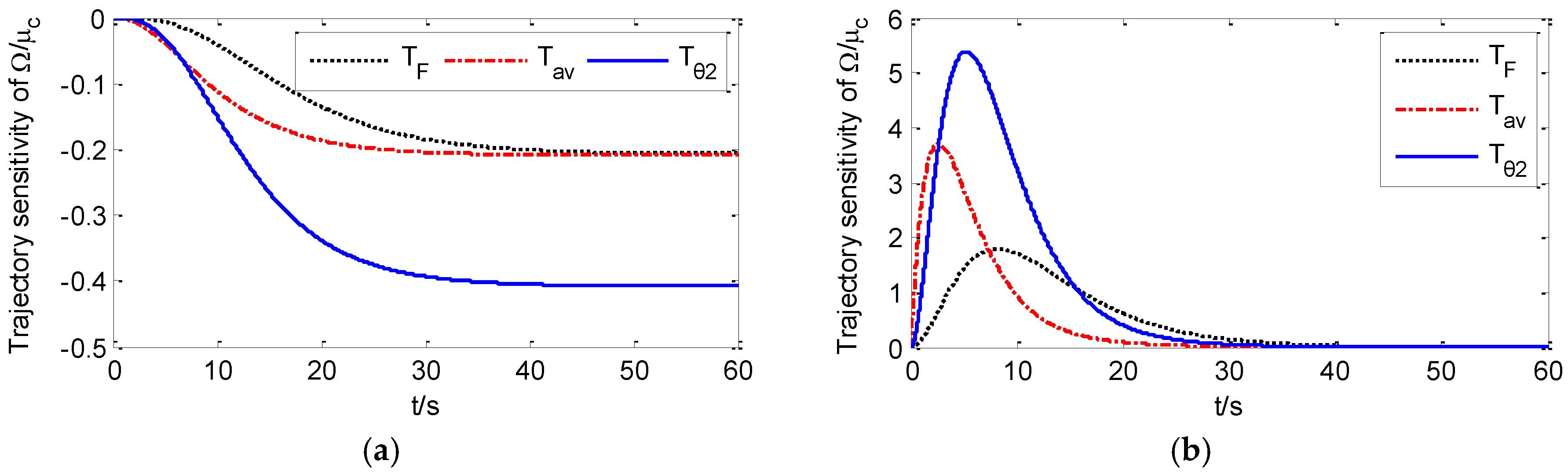
4.3. Parameter Sensitivity Analysis

The parameters should be kept in a suitable range to ensure system transient stability. The parameter influence on the system dynamic response was revealed through the sub-module parameter sensitivity analysis under different input conditions, which gave reference for parameter identification.

Taking the core fuel and coolant temperature module for example, Figure 12 shows the trajectory sensitivity analysis results with changes of ±10% to Ω/μ_c under a step change of 0.01 for N_r, or a positive step change of 10 degrees for $T_{\theta 1}$.

The parameter influence of Ω/μ_c on output variables (i.e., T_F, T_av and $T_{\theta 2}$) existed constantly as N_r changed. The trajectory sensitivities eventually dropped to zero after about 30 s under step change of $T_{\theta 1}$ (see Figure 12). Thus, there was a significant difference in the sensitivity of Ω/μ_c to each output variable under two cases. The change of N_r was more beneficial for the parameter identification of Ω/μ_c. Similarly, some other structural and thermal parameters for the steam generator module also had a constant effect on the model output variables under given input conditions.

5. Results and Discussion

The self-stabilization of the core neutron dynamic module plays an important role in the stability of the PWR plant system. There was also further discussion about the parameter identification analysis of the core neutron dynamic module and the effect of parameter sensitivity on parameter identification.

5.1. Core Neutron Dynamic Module Parameter Sensitivity Analysis

5.1.1. Parameter Sensitivity Analysis without Temperature Feedback

The typical values of l₀, λ₀ and β₀ were 2.1 × 10⁻⁵, 0.0767 and 4.4 × 10⁻³, respectively. The initial output of N_r was 0.9. This gave changes of ±10% to l₀, λ₀ and β₀, then the trajectory curve of N_r with a step change of ρ from 0 to 0.001 at 1 s was recorded. Figure 13a shows the trajectory sensitivity analysis.

For a time period longer than 0.04 s, the trajectory sensitivity of β could be expressed by the trajectory sensitivity of λ as follows:

$$\beta =-0.9451\lambda -0.02044$$

(20)

Figure 13b shows the trajectory sensitivity curves and the fitting relationship. There was a strong linear correlation between the trajectory sensitivity curves of β and λ for a time slightly longer than 0 s. β had a larger trajectory sensitivity during the entire time, meaning that λ was more difficult identify. Furthermore, l, λ and β were changed by ±10%, ±20% and ±30% at the rated working condition. Figure 13b to Figure 13e show the trajectory sensitivity curves.

From Figure 13a–e, l and λ had greater impact on the initial time with a sudden change of ρ, but l did not affect the dynamic simulation of N_r when the time was slightly over 0 s. λ and β had a continuous opposite influence on the dynamic simulation of N_r. The trajectory sensitivity had little relation to the initial working conditions due to a lack of a non-linear link in the core neutron dynamic module. In addition, the impact of l and λ on N_r did not change with the parameter disturbance depths, but β had a larger effect on the simulation result with a bigger parameter disturbance depth.

5.1.2. Parameter Sensitivity Analysis with One Loop Temperature Feedback

The core neutron dynamic module has fuel temperature and coolant temperature feedbacks with the total feedback coefficient being negative, which is necessary to ensure the reactor self-stability. Supposing the temperature feedback was reduced to one-loop, it could be expressed by the first-order inertia link as follows:

$$H\left(s\right)=\frac{a}{s+d}\times RD$$

(21)

where a and d are the constant coefficients. RD is the temperature feedback coefficient. The transfer function analysis of the core neutron dynamic module with one-loop feedback showed that the reactor temperature feedback coefficient change would change the model gain. It also showed that it would change the model output N_r under the same input of ρ.

With typical parameters, it gave changes of ±10% to l, λ, β and RD, respectively, under a step change of ρ from 0 to 0.001 at 0 s. Then, it recorded the trajectory curve of N_r. Figure 14 shows the trajectory sensitivity analysis.

From Figure 13 and Figure 14, the track sensitivities of β and λ first became larger due to the effect of the negative temperature feedback. Then, eventually the track sensitivities tended to zero at about 90 s. The effect of RD always existed with its value reducing gradually from 0, indicating that the temperature feedback coefficient had an evident effect on the steady-state value of N_r.

To summarize, the reactor temperature feedback coefficient, as well as some design parameters actually changed the model gain. As a result, the output variable steady-state values were changed with the trajectory sensitivities constantly existing. Meanwhile, the effects of other parameters were only reflected in the variation process with the trajectory sensitivities eventually reduced to zero. The trajectory sensitivity analysis of parameters could generally reflect the influence of parameters on the system dynamic response and provide a reference for the parameter identifiability. The parameter was easier to be identified if the parameter trajectory sensitivity had a large value over a long time interval. On the contrary, it was not conducive to parameter identification.

5.2. Identification Discuss of Core Neutron Dynamic Module

5.2.1. Influence of the Tested Data

For core neutron dynamic module, the identification results under two kinds of situations were further analyzed.

(a) In the case of tested data with random noise

Assuming that the tested data contained random noise with the maximum noise value reached 3% of its steady value, the parameters of the core neutron dynamic module without temperature feedback were identified. β and l could be well identified, whereas when λ was slightly different from the given value, the identification result was acceptable (see Figure 15).

(b) Input signal related to β

For the core neutron dynamic module without temperature feedback, the input signal was 0.01 multiplied by β. In this case, λ and the parameter β divided by l could be identified well. However, β and l were difficult to obtain since the parameter β divided by l could be simplified as one parameter from the differential equation of the core neutron dynamic module in Section 2. The correlation between β and l did not affect the identification of other parameters such as λ that were not associated with them.

5.2.2. Identification of Temperature Feedback Coefficient for the Core Neutron Dynamic Module

Given the power set a step change from 1 to 0.9 at 1 s, the fuel temperature and the coolant temperature feedback coefficients could be identified assuming that β, λ and l were already known. The identification of five parameters (i.e., β, λ, l, α_F and α_C) of the three-input single-output core neutron dynamic module was attempted using the RP-PSO algorithm with the parameter scope of 1 × 10⁻⁸ to 1.

Table 3. Model parameters for core neutron dynamic module.

Parameter	Value	Identified
l	2.1 × 10−5 s	8.30 × 10−6 s
β	4.4 × 10−3	0.02529
λ	0.0767 s−1	0.07666 s−1
αF	−5.81 × 10−6	−5.8080 × 10−6
αC	−9.81 × 10−5	−9.8085 × 10−5

listed the parameters for core neutron dynamic module. Figure 16 showed the comparison results after identification.

As the power set was reduced, the control rod insertion decreased the reactivity. N_r decreased rapidly with instantaneous change of T_F, and then slowly raised to 0.9. T_av firstly presented an increasing trend (see Figure 16).

The RP-PSO was compared with two other algorithms namely PSO and CPSO (i.e., the cooperative particle swarm optimization algorithm) [26]. Figure 17 shows the fitness function distribution of optimization solutions with three kinds of identification algorithms.

Due to the orders of magnitude (i.e., for the parameters to be identified were far less than 1), the PSO and CPSO algorithms were easier to cause a certain parameter to reach the set boundary value of 1 × 10⁻⁸ with the fitness function value reaching about a negative 6 order of magnitude (see Figure 17). The identification results of these two algorithms were bad. However, the RP-PSO algorithm produced some better results with the fitness function value of one group solution reaching a negative 11 order of magnitude. For this group of solution, the simulation results were acceptable (see Figure 17). The identified parameters of α_F, α_C and λ were consistent with the real value. However, β and l were slightly different from their real values since the input signal of ρ was related to β, which affected the identification as analyzed in Section 5.2.1. From the above analysis, it could also be concluded that, to a certain extent, the parameter scope might affect the optimization results of the algorithm.

The identification process that would obtain five parameters provided a way to get appropriate core neutron dynamic module parameters using the measured data of various working conditions, or under different fuel life cycles. Also through the identification based on the integrated primary loop system model, the temperature feedback coefficients had a significant effect on the identification results.

5.3. Model Adaptation

The adaptability of the established integrated model was analyzed through the comparison with the PCTRAN software, which mainly analyzed the primary loop system variables with data that was sampled at a frequency of 5 s per point. Assuming that the power set value stepped from 1 to 0.9 in 1 s, Figure 18 showed the simulation results with a nuclear power unit model connected to the single machine infinite power system. The curves in Figure 18 marked by the triangle were obtained with PCTRAN.

The thermal power of the reactor was approximated by N_r. The power set value change leads to the valve opening closure and the decrease of turbine mechanical power. The reactor core fuel temperature and the coolant average temperature were also reduced as the core power was controlled at about 0.9 p.u (see Figure 18).

6. Conclusions

The electrical, temperature and pressure variables with clear physical meaning were integrated in the primary loop system model using a modular modeling method, which reflected the actual operating characteristics. The PWR primary loop system had the characteristics of orders of magnitude that ranged from −5 to 7 for parameters and variables with a time scale of more than 300 s, which increased the parameter identification difficulty. The sampling frequency should be increased to record the rapid transition process in actual tests. Different disturbance depths under multiple conditions should be applied to get the test data, especially in case of signals with noise. The model practicability was increased by the variable initialization based on the differential equation and program setting method. The parameters were obtained from calculation or identification with the RP-PSO algorithm and were checked under various working conditions.

The trajectory sensitivities of the same parameter to the output variables under various input disturbances might be quite different for a MIMO system. Thus, the design of the appropriate test conditions was beneficial to parameter identification. The linear correlation between the trajectory sensitivities of different parameters made the parameter identifiability worse. However, the relevance parameters did not affect the identification of other parameters that were not associated with them. The parameters that changed the model gain, like the reactor temperature feedback coefficients and some other design parameters, had a more significant effect on the simulation results. These parameters needed to be obtained properly, since large deviations from their real values changed the output variable steady-state values. Meanwhile, the effects of some other parameters were only reflected in the variation process.

The parameter identification features of the advanced PWR primary loop system and the parameter identifiability difficulty degree through sensitivity analysis was helpful for the test-work design. It also laid the foundation for the calculation and identification of the model parameters based on measured data.

References

1. Maldonado, G.I. The performance of North American nuclear power plants during the electric power blackout of August 14, 2003. In Proceedings of the Nuclear Science Symposium Conference, Rome, Italy, 16–22 October 2004.
2. Kirby, B.; Kueck, J.; Leake, H.; Muhlheim, M. Nuclear generating stations and transmission grid reliability. In Proceedings of the 39th North American Power Symposium, Las Cruces, NM, USA, 30 September–2 October 2007.
3. Osborne, D.R.; Hou, J.; Graves, G.; Miller, L.F. Development of a modern pressurized water reactor simulator: Instrumentation, design and data acquisition. In Proceedings of the IEEE Nuclear Science Symposium Conference, Honolulu, HI, USA, 26 October–3 November 2007.
4. Cheng, Y.H.; Shih, C.; Chiang, S.C.; Weng, T.L. Introducing PCTRAN as an evaluation tool for nuclear power plant emergency responses. Ann. Nucl. Energy 2012, 40, 22–129. [Google Scholar] [CrossRef]
5. Ichikawa, T.; Inoue, T. Light water reactor plant modeling for power system dynamic simulation. IEEE Trans. Power Syst. 1988, 3, 463–471. [Google Scholar] [CrossRef]
6. Inoue, T.; Ichikawa, T.; Kundur, P.; Hirsch, P. Nuclear plant models for medium-to-long term power system stability studies. IEEE Trans. Power Syst. 1995, 10, 141–148. [Google Scholar] [CrossRef]
7. Hu, X.; Zhang, X.; Zhou, X.; Gan, F.; Zong, W. Pressurized water reactor nuclear power plant (NPP) modelling and the midterm dynamic simulation after NPP has been introduced into power system. In Proceedings of the IEEE Region 10 Conference on Computer, Communication, Control and Power Engineering, Beijng, China, 19–21 October 1993.
8. Wu, G.; Ju, P.; Song, X.; Xie, C.; Zhong, W. Interaction and coordination among nuclear power plants, power grids and their Protection Systems. Energies 2016, 9, 306. [Google Scholar] [CrossRef]
9. Zhao, J.; Liu, D.; Ouyang, L.; Sun, W.; Wang, Q.; Yang, N. Analysis of the mutual interaction between large-scale pressurized water reactor nuclear power plants and power systems. Proc. CSEE 2012, 32, 64–70. [Google Scholar]
10. Dong, Z. A neural-network-based nonlinear adaptive state-observer for pressurized water reactors. Energies 2013, 6, 114–119. [Google Scholar] [CrossRef]
11. Abdio, M.A. Optimal design of power system stabilizers using particle swarm optimization. IEEE Trans. Energy Convers. 2002, 17, 406–413. [Google Scholar] [CrossRef]
12. Hsu, Y.Y.; Liu, C.S.; Luor, T.S.; Chang, C.L. Experience with the identification and tuning of excitation system parameters at the second nuclear power plant of Taiwan power company. IEEE Trans. Power Syst. 1996, 11, 747–753. [Google Scholar]
13. Yu, D.; Yu, X.; Chen, F.; Chen, C. Modeling and parameter measurement research pressurized water reactor nuclear power generator’s prime mover and governor. In Proceedings of the International Conference on Power System Technology, Chengdu, China, 20–22 October 2014.
14. Sage, A.P.; Masters, G.W. Identification and modeling of states and parameters of nuclear reactor systems. IEEE Trans. Nucl. Sci. 1967, 279–285. [Google Scholar] [CrossRef]
15. Gábor, A.; Fazekas, C.; Szederkényi, G.; Hangos, K.M. Modeling and identification of a nuclear reactor with temperature effects and Xenon poisoning. Eur. J. Control 2009, 17, 104–115. [Google Scholar] [CrossRef]
16. Fazekas, C.; Szederkényi, G.; Hangos, K.M. Parameter estimation of a simple primary circuit model of a VVER plant. IEEE Trans. Nucl. Sci. 2008, 55, 2643–2743. [Google Scholar] [CrossRef]
17. Carlos, S.; Ginestar, D.; Martorell, S.; Serradell, V. Parameter estimation in thermalhydraulic models using the multidirectional search method. Ann. Nucl. Energy 2003, 30, 133–158. [Google Scholar] [CrossRef]
18. Cadini, F.; Zio, E. A Monte Carlo method for the model-based estimation of nuclear reactor dynamics. Ann. Nucl. Energy 2007, 34, 773–781. [Google Scholar] [CrossRef]
19. Embrechts, M.J.; Benedek, S. Hybrid identification of nuclear power plant transients with artificial neural networks. IEEE Trans. Ind. Electron. 2004, 51, 686–693. [Google Scholar] [CrossRef]
20. Khoshahval, F.; Minuchehr, H.; Zolfaghari, A. Performance evaluation of PSO and GA in PWR core loading pattern optimization. Nucl. Eng. Des. 2011, 241, 799–808. [Google Scholar] [CrossRef]
21. Waintraub, M.; Schirru, R.; Pereira, C.M.N.A. Multiprocessor modeling of parallel particle swarm optimization applied to nuclear engineering problems. Prog. Nucl. Energy 2009, 51, 680–688. [Google Scholar] [CrossRef]
22. Medeiros, J.A.C.C.; Schirru, R. Identification of nuclear power plant transients using the Particle Swarm Optimization algorithm. Ann. Nucl. Energy 2008, 35, 576–582. [Google Scholar] [CrossRef]
23. Pereira, C.M.N.A.; Lapa, C.M.F.; Mol, A.C.A.; Luz, A.F.D. A particle swarm optimization (PSO) approach for non-periodic preventive maintenance scheduling programming. Prog. Nucl. Energy 2010, 52, 710–714. [Google Scholar] [CrossRef]
24. Li, Y.; Ma, J.; Chan, A.; Huang, Y.; Wang, B. Mechanism model of pressurizer in the pressurized water reactor nuclear power plant based on PSO algorithm. In Proceedings of the 24th Control & Decision Conference, Taiyuan, China, 23–25 May 2012.
25. Tang, L.; Mccalley, J. Trajectory sensitivities: Applications in power systems and estimation accuracy refinement. In Proceedings of the IEEE Power & Energy Society General Meeting, Vancouver, BC, Canada, 21–25 July 2013.
26. Li, X.; Yao, X. Cooperatively coevolving particle swarms for large scale optimization. IEEE Trans. Evol. Comput. 2012, 16, 210–224. [Google Scholar]
Figure 1. AP1000 system model diagram.
Energies 10 00173 g001
Figure 2. Reactor power control system module. (a) Reactor power control system diagram; (b) average temperature link; (c) variable amplification link; and (d) nonlinear amplification link. Tref is the given temperature value for the reactor.
Energies 10 00173 g002aEnergies 10 00173 g002b
Figure 3. System diagram of steam turbine module. FHP and FLP are the proportional coefficients of high-pressure cylinder and low-pressure cylinder, respectively. λh is the overshooting coefficient. TCH, TRH and TCO are the volume time constants.
Energies 10 00173 g003
Figure 4. System diagram of governor model. ω is the generator speed unit. K is the proportional coefficient. TR1 is the measurement inertia time constant. KP, KI and KD are the proportional, integral and differential coefficients, respectively.
Energies 10 00173 g004
Figure 5. Electro-hydraulic servo system model.
Energies 10 00173 g005
Figure 6. Steam turbine bypass control system diagram.
Energies 10 00173 g006
Figure 7. Nuclear power parameter identification process. (a) Nuclear power parameter identification process diagram; and (b) parameter identification process diagram with the random perturbation particle swarm optimization (RP-PSO) and Simulink.
Energies 10 00173 g007
Figure 8. Core neutron dynamic module simulation comparison. (a) Fitness function change with optimization iterations; (b) change of β with optimization iterations; (c) change of λ with optimization iterations; (d) change of l with optimization iterations; and (e) simulation comparison of Nr.
Energies 10 00173 g008
Figure 9. Core fuel and coolant temperature module simulation comparison. (a) Change of TF; (b) change of Tθ2; and (c) change of Tav.
Energies 10 00173 g009aEnergies 10 00173 g009b
Figure 10. Reactor power control module simulation comparison.
Energies 10 00173 g010
Figure 11. Steam generator module simulation comparison. (a) Input change of THL; (b) output change of TCL; and (c) output change of Ps.
Energies 10 00173 g011
Figure 12. Sensitivity of parameter change to the output variables under two different cases. (a) Sensitivity analysis of Ω/μc under input change of Nr; and (b) sensitivity analysis of Ω/μc under input change of T θ 1 .
Energies 10 00173 g012
Figure 13. Sensitivity analysis of parameter change without temperature feedback. (a) Trajectory sensitivity with parameter disturbances of ±10%; (b) fitting relationship between the trajectory sensitivity of β and λ; (c) trajectory sensitivity with different disturbance depths for l; (d) trajectory sensitivity with different disturbance depths for λ; and (e) trajectory sensitivity with different disturbance depths for β.
Energies 10 00173 g013
Figure 14. Sensitivity analysis of parameter change with one-loop temperature feedback.
Energies 10 00173 g014
Figure 15. Comparison results tested data in case of tested data with random noise. (a) Input signal with random noise; and (b) simulation comparison of Nr with random noise.
Energies 10 00173 g015
Figure 16. Comparison results of the core neutron dynamic module. (a) Input change of ρ; (b) input change of TF; (c) input change of Tav; and (d) output change of Nr.
Energies 10 00173 g016
Figure 17. Fitness function value distribution of optimization solutions for three kinds of identification algorithms.
Energies 10 00173 g017
Figure 18. Response of AP1000 with power disturbance. (a) Change of TF; (b) change of reactor thermal power; (c) change of Tavg; (d) change of Ps; and (e) change of Pm.
Energies 10 00173 g018