Article

An Artificial Neural Network for Analyzing Overall Uniformity in Outdoor Lighting Systems

by
Antonio Del Corte-Valiente
1,*,
José Luis Castillo-Sequera
2,
Ana Castillo-Martinez
2,
José Manuel Gómez-Pulido
2 and
Jose-Maria Gutierrez-Martinez
2
1
Department of Computer Engineering, Polytechnic School, University of Alcala, 28871 Alcalá de Henares, Spain
2
Department of Computer Sciences, Polytechnic School, University of Alcala, 28871 Alcalá de Henares, Spain
*
Author to whom correspondence should be addressed.
Energies 2017, 10(2), 175; https://doi.org/10.3390/en10020175
Submission received: 18 October 2016 / Revised: 19 January 2017 / Accepted: 20 January 2017 / Published: 4 February 2017

Abstract

:
Street lighting installations are an essential service for modern life due to their capability of creating a welcoming feeling at nighttime. Nevertheless, several studies have highlighted that it is possible to improve the quality of the light significantly improving the uniformity of the illuminance. The main difficulty arises when trying to improve some of the installation’s characteristics based only on statistical analysis of the light distribution. This paper presents a new algorithm that is able to obtain the overall illuminance uniformity in order to improve this sort of installations. To develop this algorithm it was necessary to perform a detailed study of all the elements which are part of street lighting installations. Because classification is one of the most important tasks in the application areas of artificial neural networks, we compared the performances of six types of training algorithms in a feed forward neural network for analyzing the overall uniformity in outdoor lighting systems. We found that the best algorithm that minimizes the error is “Levenberg-Marquardt back-propagation”, which approximates the desired output of the training pattern. By means of this kind of algorithm, it is possible to help to lighting professionals optimize the quality of street lighting installations.

1. Introduction

Street lighting has become in an essential service for modern life. These kinds of installations are responsible of creating a welcoming feeling, making it possible to increment the night activity while reducing crime at the same time [1,2]. Despite all their helpful uses, street lighting installations are one of the highest energy consumers, accounting for up to 2.3% of the global electricity consumption [3], while also being responsible for up to 60% of the local government’s greenhouse gas emissions [4].
Nevertheless, several studies have highlighted that it is possible to reduce the energy costs up to 45% [5]. To achieve this reduction, it is necessary to study each case carefully to find the best design solution. The main problem for performing this type of study is the need to preserve the compliance with the current standards and satisfy the desired level of energy efficiency at the same time.
Several tools are used by lighting designers to make this study possible, such as AutoCAD or DIALux, among others. Their main difficulty arises when trying to optimize some of the installation’s characteristics, as the lamps or the distance between luminaires, due to the impact on multiple final factors. For that reason, it is important to define the most important parameter to optimize.
One of the parameters that must to be taken into account in the design phase in outdoor lighting systems is the overall illuminance uniformity, which allows one to perceive the environment continuously and without sudden breaks caused by lighting level drops. This factor is directly related to the quality of road illumination due to the fact that low uniformity ratios imply frequent changes between contrasting high and low lit road segments, causing eye discomfort, which in turn lead to stress and fatigue [6]. A perfect uniformity means that the luminous flux is spatially invariant. However, in practice, there is always some degree of non-uniformity in the illumination field.
Due to the high number of vehicles on roads, the severity of fatigue-related accidents has become a major concern [7]. Thereby, for the driver’s comfort and safety, decreased illumination uniformity ratios on the road are unacceptable conditions [8] because it difficult to perceive certain objects against the background [9]. However, not only the driver’s comfort and security benefit from correct lighting. It also helps to increase the security due to the well-established reduction of crime incidents in a well-lit area. Despite the importance of the uniformity in lighting, the main problem arises when, with the purpose of saving energy, half the road lamps are switched off at midnight, resulting in bad uniformity in light distribution and poor visibility [10].
Analyzing Spanish regulations regarding energy efficiency [11], a minimum overall uniformity level of 40% is recommended to ensure that lighting installations do not create dark lighting patches next to lighter light patches. Current uniformity metrics are based only on statistical analysis of the light distribution [12,13]. These approaches are good for applications where the end user is not a human, e.g., solar concentrators. However, for most applications, illumination patterns are ultimately viewed by human beings, and then the natural way of quantifying uniformity quality should be through direct observation by humans. However, this is very impractical and prone to subjective errors. The simplest approach to obtain the overall illuminance uniformity involving numeric values of illuminance of only two points on the target. The most popular of these approached is the min–max ratio.
To help in this field of street lighting optimization, this paper presents a new algorithm that is able to obtain the overall illuminance uniformity in an easy way, in order to improve the quality of lighting systems. Taking into account that feedforward neural networks have been applied successfully in many different problems since the advent of the error back-propagation-learning algorithm [14], this paper presents a new approach of using these sort of artificial neural networks to obtain the overall illuminance uniformity.
To develop this algorithm it was necessary to conduct a detailed study of all the elements which are part of the street lighting installations. With the purpose of guaranteeing that all the elements were taken into account, DIALux, one of the most powerful tools in street lighting design was used [15].
The paper is organized as follows: firstly, the most important characteristics of street lighting installations and its influence on energy efficiency were analyzed. Next, a description of the selected algorithm is presented. After that, the configuration of the algorithm parameters is shown through several experiments. To finalize, a section to summarize the most relevant conclusions obtained after the development of the algorithm is presented.

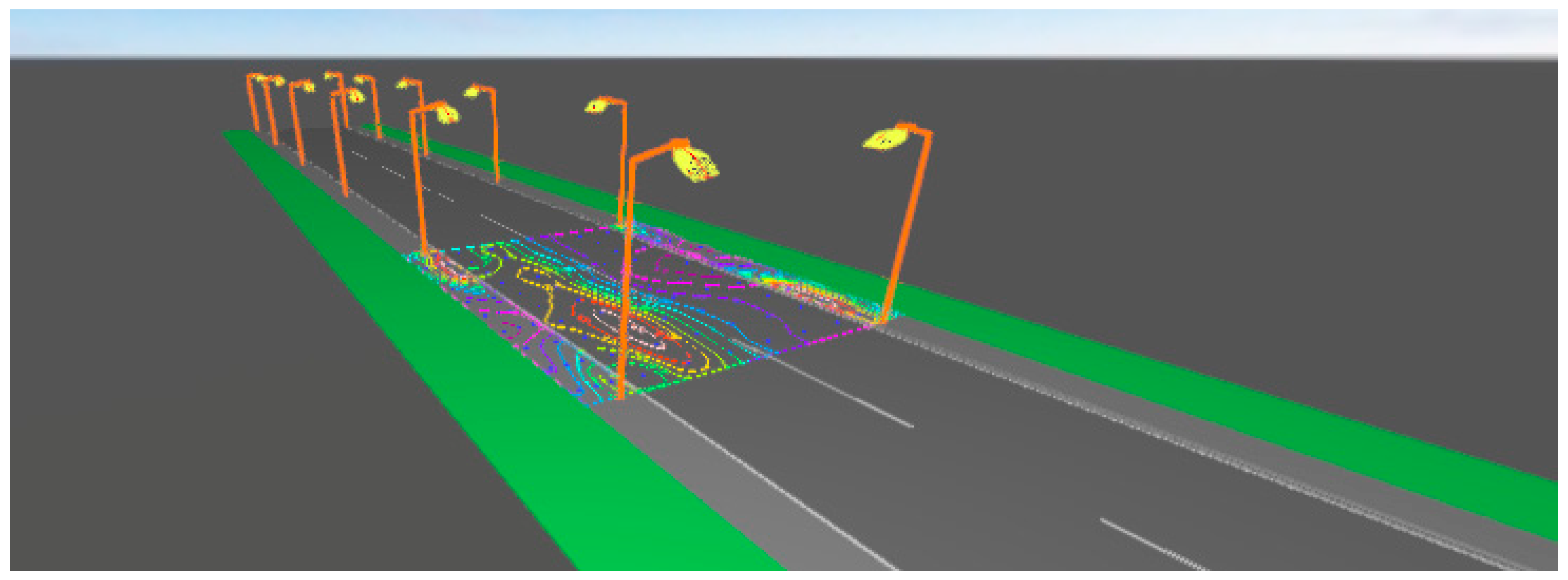
2. Street Lighting/Experimental Context

Uniformity is a ratio of the minimum illuminance level to the average illuminance level. A uniformity value of 0.4 or 40% is recommended to ensure that lighting installations do not create dark patches next to lighter patches, especially when our eyes have difficulty in adjusting quickly enough to proceed along any route. Low uniformity ratios, frequent changes of contrasting high- and low-lit road segments cause enormous eye discomfort, leading to stress and fatigue which often have a negative impact on road safety [6]. In a conventional sense, uniformity is what distinguishes a good quality road lighting installation from a poor one [16]. Thus, a good lighting system is one designed to distribute an appropriate amount of light evenly with uniformity values of between 0.25 and 0.40 using lamps with a rating of at least 60 on the Colour Rendering Index (CRI) [17].
This magnitude is influenced by several design considerations of the installations. For example, the height of street lighting poles influences how uniform the light levels are on the street and in the surrounding area [18]. The higher the mounting height, the greater the beam spread along the road and the smaller the number of mounting points required within a certain area will be. Other pay-offs from higher mounting height will enhance road surface luminance uniformity and lower glare [19]. Thus, lighting designers must take into account several considerations when designing a new installation.
Classification is one of the most important tasks in the application areas of artificial neural networks (ANNs). Training a neural network is a complex task in the supervised learning field of research. The main difficulty in adopting ANN is to find the most appropriate combination of learning, transfer and training functions for the classification task. We compared in this work the performances of six types of training algorithms in feed-forward neural network for analyzing overall uniformity in outdoor lighting systems. In this work, we have selected the following training algorithms: Levenberg-Marquadt back-propagation, scaled conjugated gradient back-propagation, gradient descent with momentum, gradient descent with adaptive learning rate back-propagation, gradient descent with momentum and adaptive learning rate back-propagation and gradient descent back-propagation with a sigmoidal activation function. We believe it is important to establish the best training algorithm to optimize some of the installation’s characteristics in outdoor lighting systems with ANN.
In our study, we used thirteen outdoor lighting system input patterns and we intended to analyze the behavior of ANN in the random selection of training patterns, validation and testing with 260 patterns from 500 simulations. Simple random sampling (SRS) is the most common method [20,21,22] to partition data. It is efficient, easy to implement and leads to low model performance bias. Samples were selected randomly with a uniform distribution. The 13 elements that characterized the data and which constituted the input pattern (training, validation and test) to the neural network included the variables shown in Table 1. All the data used in the learning process were normalized in order to have the same range. We also checked that the input data were always the same.

The Simulation Software

To obtain enough information to train and test the algorithm, the DIALux software was used in order to simulate as many cases as possible. DIALux is a free software used to design, calculate and visualize light professionally in single rooms, whole floors, buildings and outdoor scenes. DIALux is used as a planning tool by over 600,000 lighting designers worldwide. DIALux is constantly undergoing further development and meets the requirements of modern lighting design and lighting calculations. As a result, 500 different simulations were performed with different combinations of the variables showed on Table 1. Figure 1 shows one of those simulations.

3. Artificial Neural Networks

3.1. ANN Application in Lighting Systems

Neural networks, with their remarkable ability to derive meaning from complicated or imprecise data, can be used to extract patterns and detect trends that are too complex to be noticed by either humans or other computer techniques. A trained neural network can be thought of as an “expert” system. This expert can then be used to provide projections given new situations of interest and answer “what if” questions. Other advantages of artificial neural networks (ANN) include:
(1)
Adaptive learning: An ability to learn how to do tasks based on the data given for training or initial experience.
(2)
Self-Organization: An ANN can create its own organization or representation of the information it receives during learning time.
(3)
Real Time Operation: ANN computations may be carried out in parallel, and special hardware devices are being designed and manufactured which take advantage of this capability.
(4)
Fault Tolerance via Redundant Information Coding: Partial destruction of a network leads to the corresponding degradation of performance. However, some network capabilities may be retained even with major network damage.
There are many steps where the ANN can be utilized in the lighting system design both in the room index and zonal cavity methods. Some of them are commented on briefly:
(a)
Determination of the effective reflectance of ceiling, room and floor cavities: This is a preliminary requirement for the determination of coefficient of utilization in the zonal cavity method.
(b)
Determination of the coefficient of utilization (CU): The CU table is provided for the discrete values of room cavity ratio (RCR), effective reflectance of ceiling cavity (ERCC) and room cavity wall reflectance (RWR) are calculated.
(c)
Other areas of application of ANN: In a similar way, the ANN may be used for the determination of correction factors for the coefficient of utilization, utilization factor in the room index method, glare index, correction factor for glare index, direct ratios, light output ratios from polar curves, selection of lighting fixtures. illuminance at any point using photometric data and upward and downward light output ratios.

3.2. ANN Development

Because ANNs are computational models which try to simulate some properties of biological neural networks, they are composed of a number of interconnected simple processing elements called neurons or nodes. Each node receives an input signal with information from other nodes or external stimuli, processes it locally through an activation or transfer function and produces an output signal that is sent to other nodes or external outputs. Despite the fact that a single neuron could seem extremely simple, the interconnection of several neurons building a network is very powerful. Indeed, it has been shown that artificial neural networks can approximate arbitrary continuous functions making tools which can be used to model complex relationships between inputs and outputs or to find patterns in data [23]. The first step to develop an ANN is to select between the different kinds of existing networks. ANNs can be classified in four groups depending on their use:
  • Feed-forward networks: Feed-forward ANNs allow signals to travel one-way only; from input to output. There is no feedback (loops), i.e., the output of any layer does not affect that same layer. Feed-forward ANNs tend to be straightforward networks that associate inputs with outputs. They are extensively used in pattern recognition. This type of organization is also referred to as bottom-up or top-down.
  • Feedback networks: Feedback networks can have signals traveling in both directions by introducing loops in the network. Feedback networks are very powerful and can get extremely complicated. Feedback networks are dynamic; their ‘state’ is changing continuously until they reach an equilibrium point. They remain at the equilibrium point until the input changes and a new equilibrium needs to be found. Feedback architectures are also referred to as interactive or recurrent, although the latter term is often used to denote feedback connections in single-layer organizations.
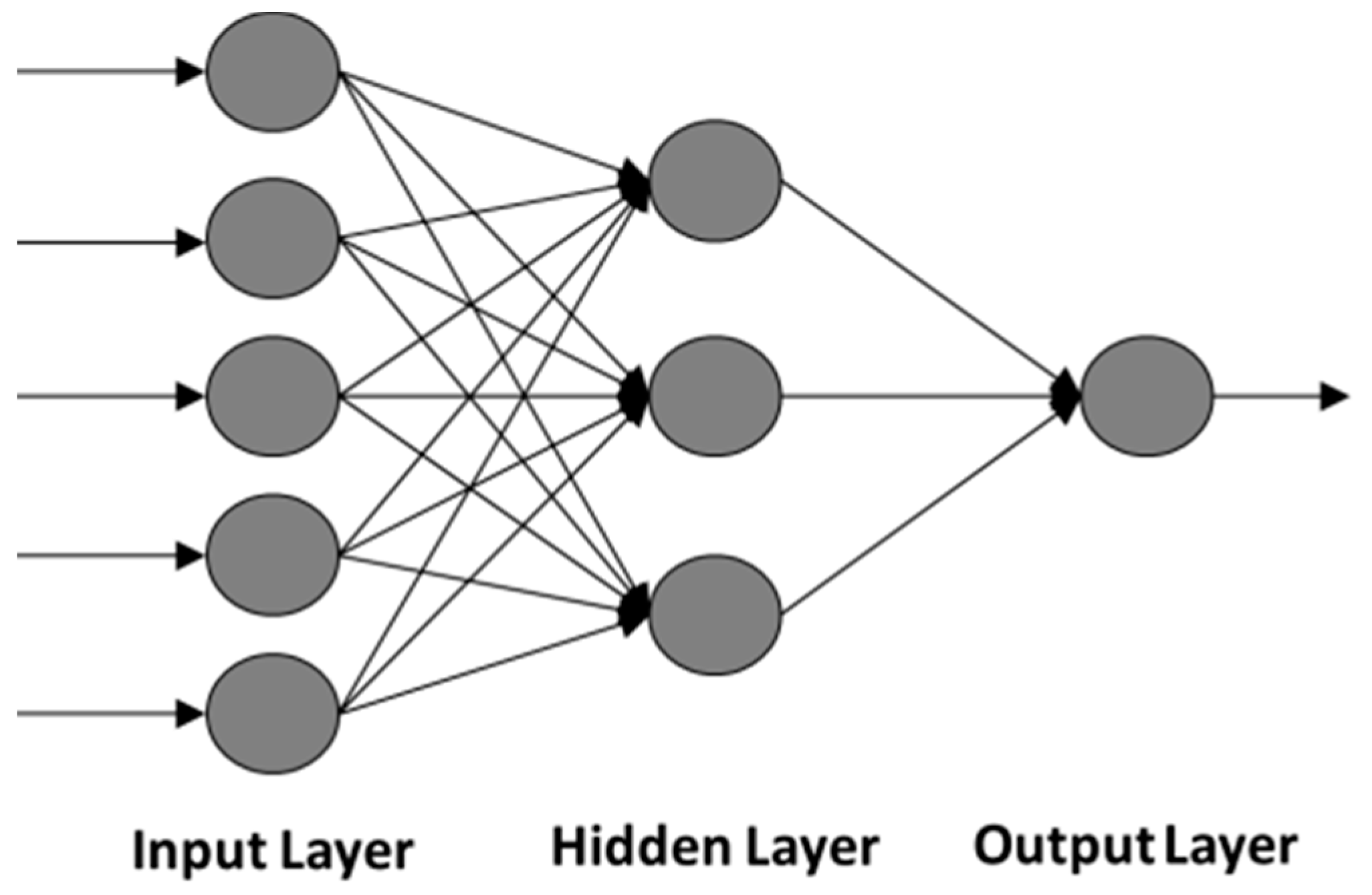
  • Network layers: The commonest type of artificial neural network consists of three groups, or layers, of units. A layer of “input” units is connected to a layer of “hidden” units, which is connected to a layer of “output” units. The activity of the input units represents the raw information that is fed into the network. The activity of each hidden unit is determined by the activities of the input units and the weights on the connections between the input and the hidden units. The behavior of the output units depends on the activity of the hidden units and the weights between the hidden and output units. This simple type of network is interesting because the hidden units are free to construct their own representations of the input. The weights between the input and hidden units determine when each hidden unit is active, and so by modifying these weights, a hidden unit can choose what it represents. We also distinguish single-layer and multi-layer architectures. The single-layer organization, in which all units are connected to one another, constitutes the most general case and is of more potential computational power than hierarchically structured multi-layer organizations. In multi-layer networks, units are often numbered by layer, instead of following a global numbering.
  • Perceptrons: The perceptron turns out to be a neuron with weighted inputs with some additional, fixed, pre-processing. Units are called association units and their task is to extract specific, localized featured from the input data. They were mainly used in pattern recognition even though their capabilities extended a lot more.

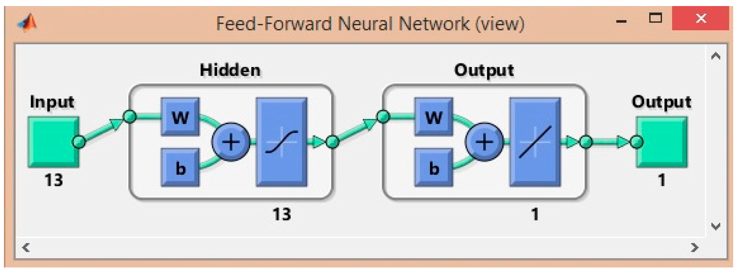
3.3. Feedforward Neural Network (FNN)

Feedforward ANNs are currently being used in a variety of applications with great success, mainly, due to its capability to learn from examples being not necessary to specify the problem to solve. This ability makes ANN able to identify and respond to patterns that are similar but not identical to the ones they have been trained. Nonetheless, the main drawback of this kind of ANNs is that there is not guarantee that the model will perform well for the problem at hand [24].
Therefore, the development of an ANN’s consists in the search of the best configuration of the four elements that comprise its architecture [25]:
  • The number of layers
  • The number of neurons in each layer
  • The activation function
  • The training algorithm (because this determines the final value of the weights and biases).
The feedforward neural network is a particular network where all the layers are linked to each other and where the information is elaborated by neurons in only one direction. When an input layer is defined, one or more hidden layers, and one output one you are defining a particular architecture of ANN generally called multi-layer perceptron (MLP) which is a particular feedforward neural network pattern. The MLP is the architecture (the number of layers) defined for the ANN. When the ANN is trained it is necessary to choose the available learning process which allows one to minimize the error function and to modify the weight matrix of the neuron connections. In order to optimize the velocity of the learning process, which is, all the processes related to the implementation of ANN (training, validation, and test), different algorithms for the transfer function can be defined in the neurons. This transfer function is used for the gradient calculation of the error function; if the sigmoidal function is chosen, the learning process is faster thanks to the simplification arising from the calculation of the gradient function. The Matlab tools mean squared error (MSE) and Regression allow calculating all the control parameters, therefore all the results obtained in terms of these parameters depend on all these factors. For these reasons, this kind of ANN has been selected to solve the problem of obtain the overall street lighting uniformity. Next, the study of the best elements setting for each of the above features in FNN is shown.

3.4. Number of Layers

A multilayer perceptron network (MPN) consists of an input layer, one or more hidden layers of computation nodes, and an output layer. Figure 2 shows a typical feed-forward network with one hidden layer consisting of three nodes, five input neurons and one output.
Studying in depth the number of layers needed there is no doubt that the selected network needs at least two layers, one for the street lighting characteristics inputs and one for the overall uniformity output. To find the best configuration for the hidden layers, some studies show how a single hidden layer is enough for ANNs to approximate a complex nonlinear function, the reason why most authors use this configuration for forecasting purposes [26,27]. However, a two hidden layer networks may provide more benefits for some type of problems [28]. On the other hand, studies have concluded that a network never needs more than two hidden layers to solve most problems [29,30]. As can be seen, the issue of determining the optimal number of hidden nodes is crucial and complicated. Despite the fact networks with fewer hidden nodes are preferable due to their better generalization ability and less over-fitting problems, networks with too few hidden nodes may not have enough power to solve the problem. As there is no theoretical basis for selecting this network characteristic, the configuration selected to solve the proposed problem is three layers, one input layer, one hidden layer and one output layer.

3.5. Number of Neurons in Each Layer

As we saw in the previous section, the proposed ANN has three different layers. In the case of the input layer there is no doubt that the number of nodes must be equal to the number of street lighting installation characteristics, that in our case is composed of 13 different parameters. In the case of the output, the number of nodes must be equal to the number of desired parameters, which in our case is one, the overall uniformity. However, the number of nodes of the hidden layer requires a previous study that may help determine the best configuration.
To determine the number of hidden nodes, the most common practice is through experiments, where several configurations are compared, or by trial-and-error. Nonetheless, some rules of thumb have been proposed. If we pay attention to the studies carried out with one hidden layer networks, we can find different existing guidelines such as “2n + 1” [31], “2n” [32], “n” [33] or, “n/2” [34], where n is the number of input nodes. Although it is impossible to generalize to one of these proposals due to the fact none of these choices work for all problems, several studies have shown how networks with the same number of hidden nodes as input nodes have better forecasting results [32,35]. For that reason, we have decided to set this number of hidden nodes to the final network.

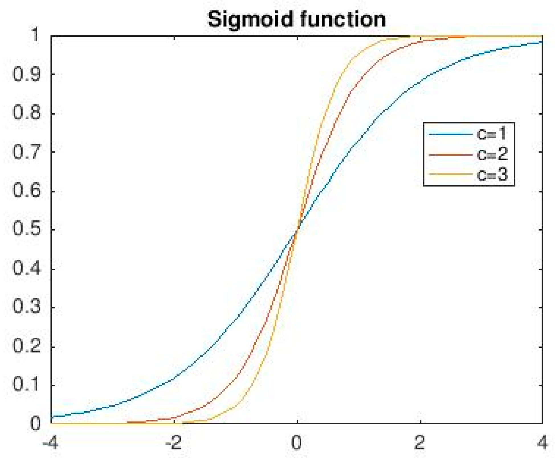
3.6. Activation Function of Each Layer

The more popular activation functions for feed forward networks is the sigmoid, a real function Sc: R → (0, 1) defined by the expression:
S c ( x ) =   1 1 + e c x
The constant c can be selected arbitrarily and its reciprocal 1/c is called the temperature parameter in stochastic neural networks. The shape of the sigmoid changes according to the value of c, as can be seen in the Figure 3.
The graph shows the shape of the sigmoid for c = 1, c = 2 and c = 3. Higher values of c bring the shape of the sigmoid closer to that of the step function and in the limit, c → ∞ the sigmoid converges to a step function at the origin.

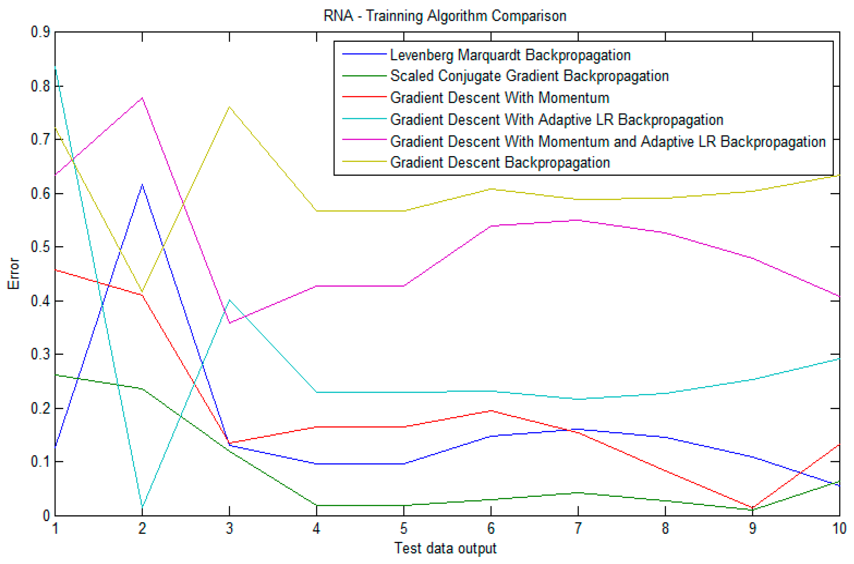
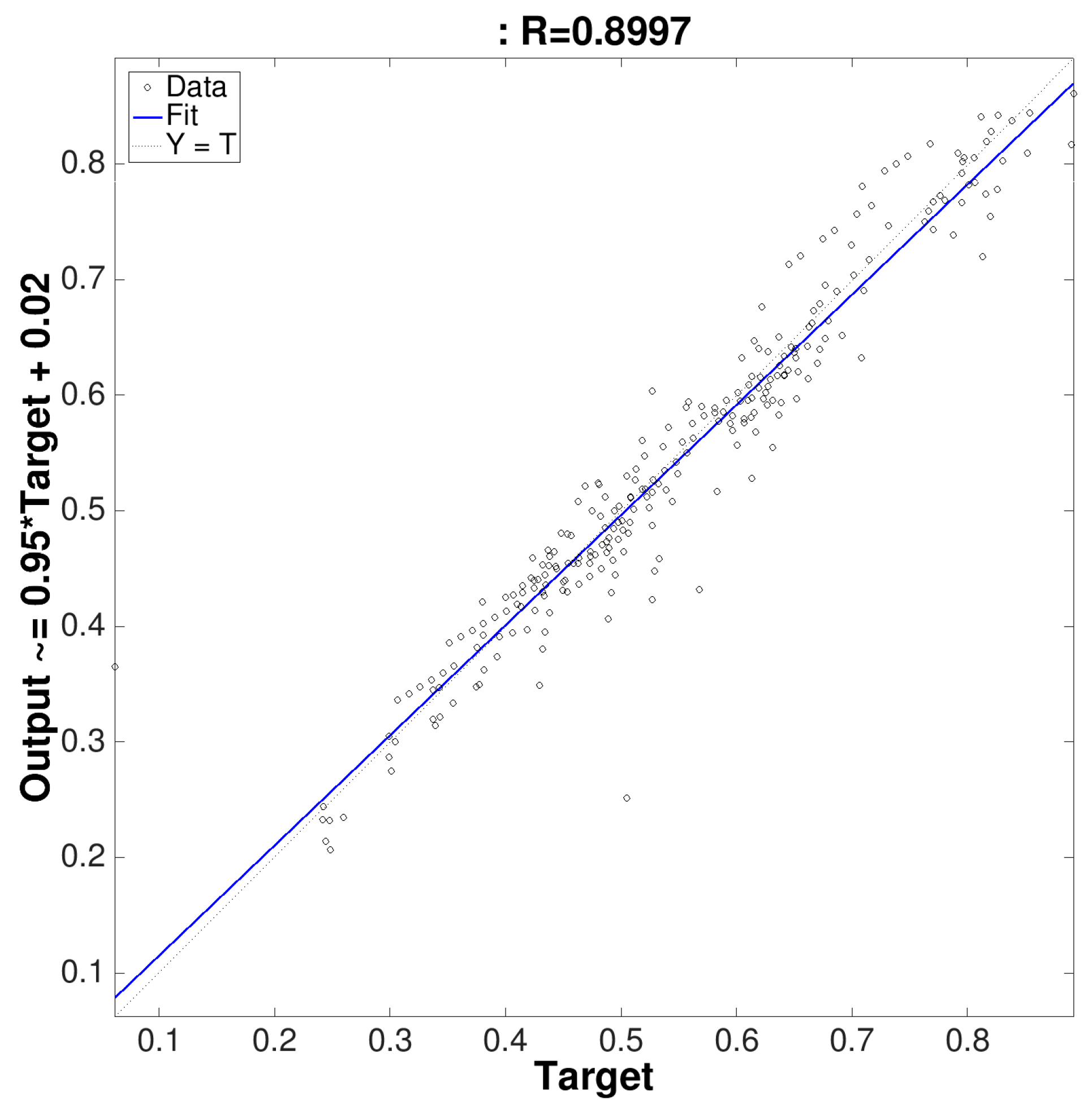
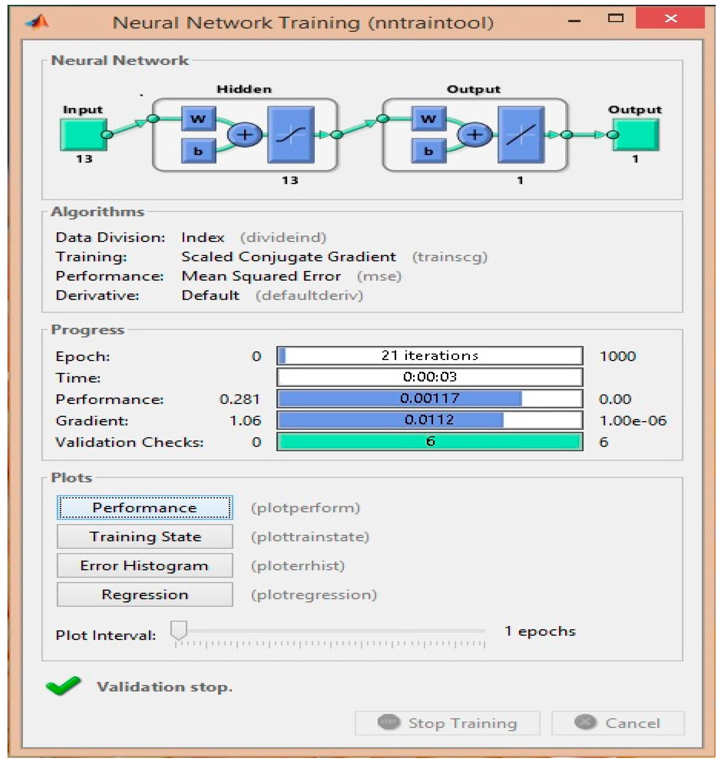
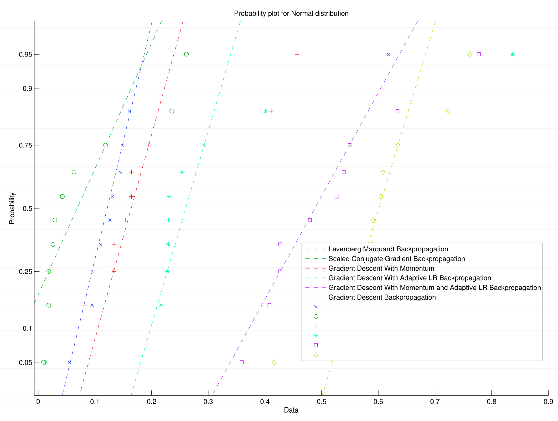
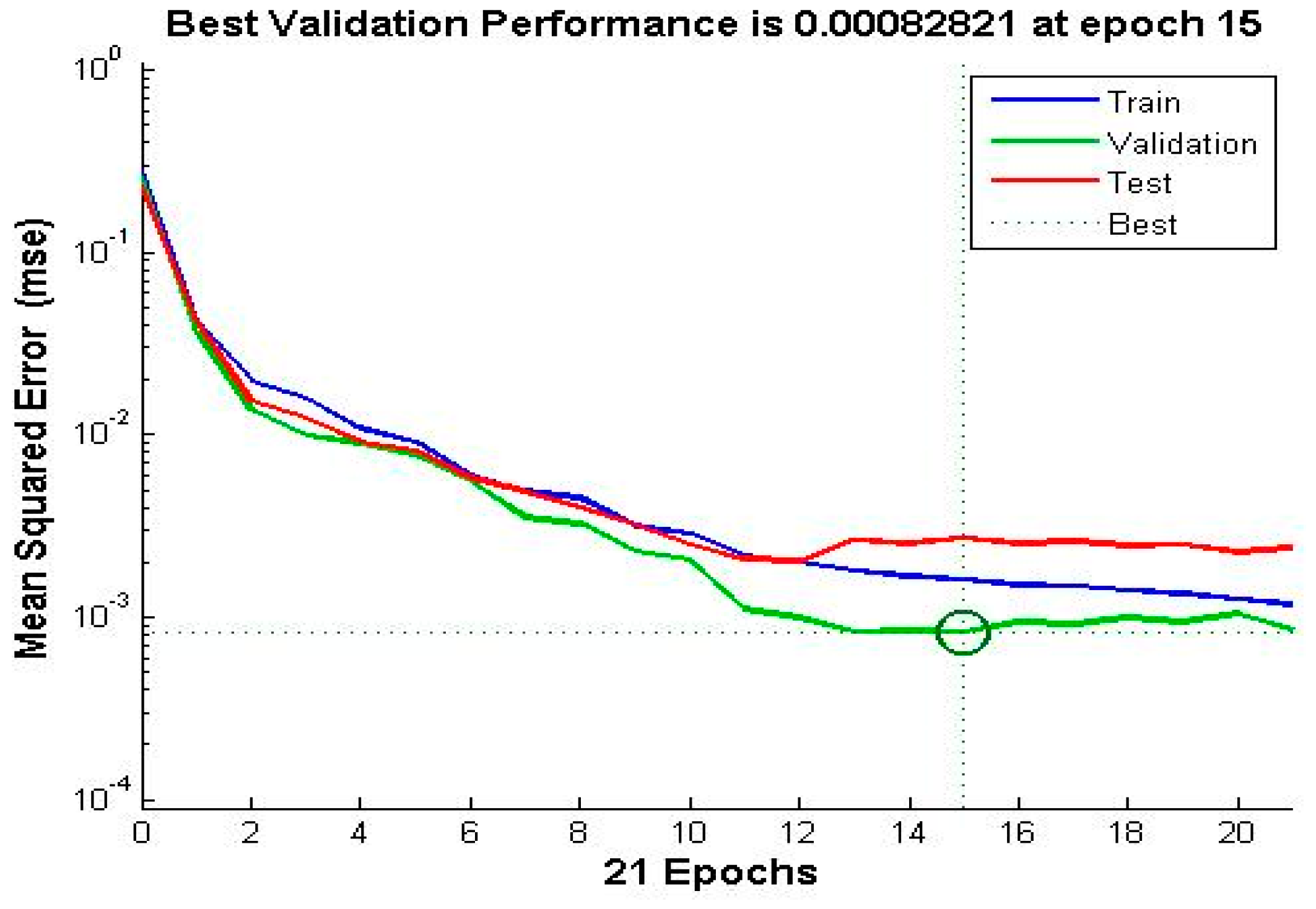
3.7. Training Algorithm

The existence of different training algorithms, where is no single one can guarantee the global optimal solution, provides various choices for neural network training. For that reason, and in order to identify the best option for the proposed algorithm, several training algorithms were used.

3.7.1. Levenberg-Marquadt Back-Propagation

The Levenberg-Marquardt algorithm (LMA), also known as the damped least-squares (DLS) method, is an iterative technique that locates the minimum of a multivariate function that is expressed as the sum of squares of non-linear real-valued functions [36]. It has become a standard technique for non-linear least-squares problems [37], widely adopted in a broad spectrum of disciplines. LMA can be thought of as a combination of steepest descent and the Gauss-Newton method. When the current solution is far from a local minimum, the algorithm behaves like a steepest descent method: slow, but guaranteed to converge. When the current solution is close to a local minimum, it becomes a Gauss-Newton method and exhibits fast convergence [38]:
F ( w ) = p = 1 P k = 1 K ( d k p o k p ) 2
where d k p is the desired value of the k-th output at the p-th pattern, o k p is the actual value of the k-th output at the p-th pattern, P is the number of patterns, and K is the number of the network outputs [39].

3.7.2. Scaled Conjugated Gradient Back-Propagation

Scaled conjugate gradient (SCG) is a second order conjugate gradient algorithm that helps to minimize goal functions or several variables. This theoretical foundation was prove by Moller [40], who used first order techniques in first derivatives like standard back-propagation and found a better way to a local minimum in second order techniques in second derivatives. The SCG training algorithm was developed to avoid this time-consuming line search, thus significantly reducing the number of computations performed in each iteration, although it may require more iterations to converge than the other conjugate gradient algorithms [40].

3.7.3. Gradient Descent with Momentum

The gradient descent with momentum (GDM) algorithm is the steepest descent with momentum that allows a network to respond to the local gradient as well as recent trends in the error surface. It acts like a low-pass filter that means that with momentum the network ignores small features in the error surface. A network can get stuck into a shallow local minimum but with momentum it slides through such local minima [41].

3.7.4. Gradient Descent with Adaptive Learning Rate Back-Propagation

The gradient descent with adaptive (GDA) algorithm was developed to allow the learning rate parameter to be adaptive to keep the learning step size as large as possible while maintaining learning stability. In the GDA algorithm, the optimal value of the learning rate parameter changes with the gradient’s trajectory on the error surface [42].

3.7.5. Gradient Descent with Momentum and Adaptive Learning Rate Back-Propagation

The gradient descent with momentum and adaptive learning rate algorithm can train any network as long as its weight, net input, and transfer functions have derivative functions [43]. This method uses back-propagation to calculate the derivative of the performance cost function with respect to the weight and bias variables of the network. Each variable is adjusted according to the gradient descent with momentum. For each step of the optimization, if performance decreases the learning rate is increased. This is probably the simplest and most common way to train a network [14].

3.7.6. Gradient Descent Back-Propagation

The gradient descent back-propagation learning algorithm is the basic one permitting stable training. This algorithm updates the weights and biases of artificial neural nets in the direction of the negative gradient of the performance function with a pre-set learning rate. This can cause a very slow training when the gradient has a small magnitude [44].

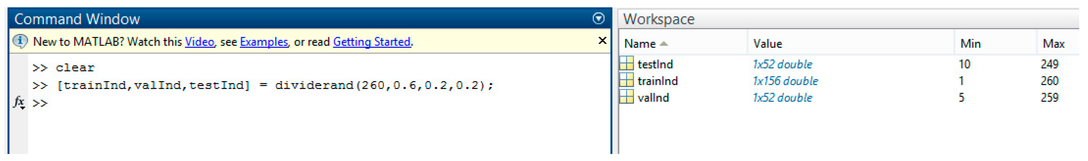
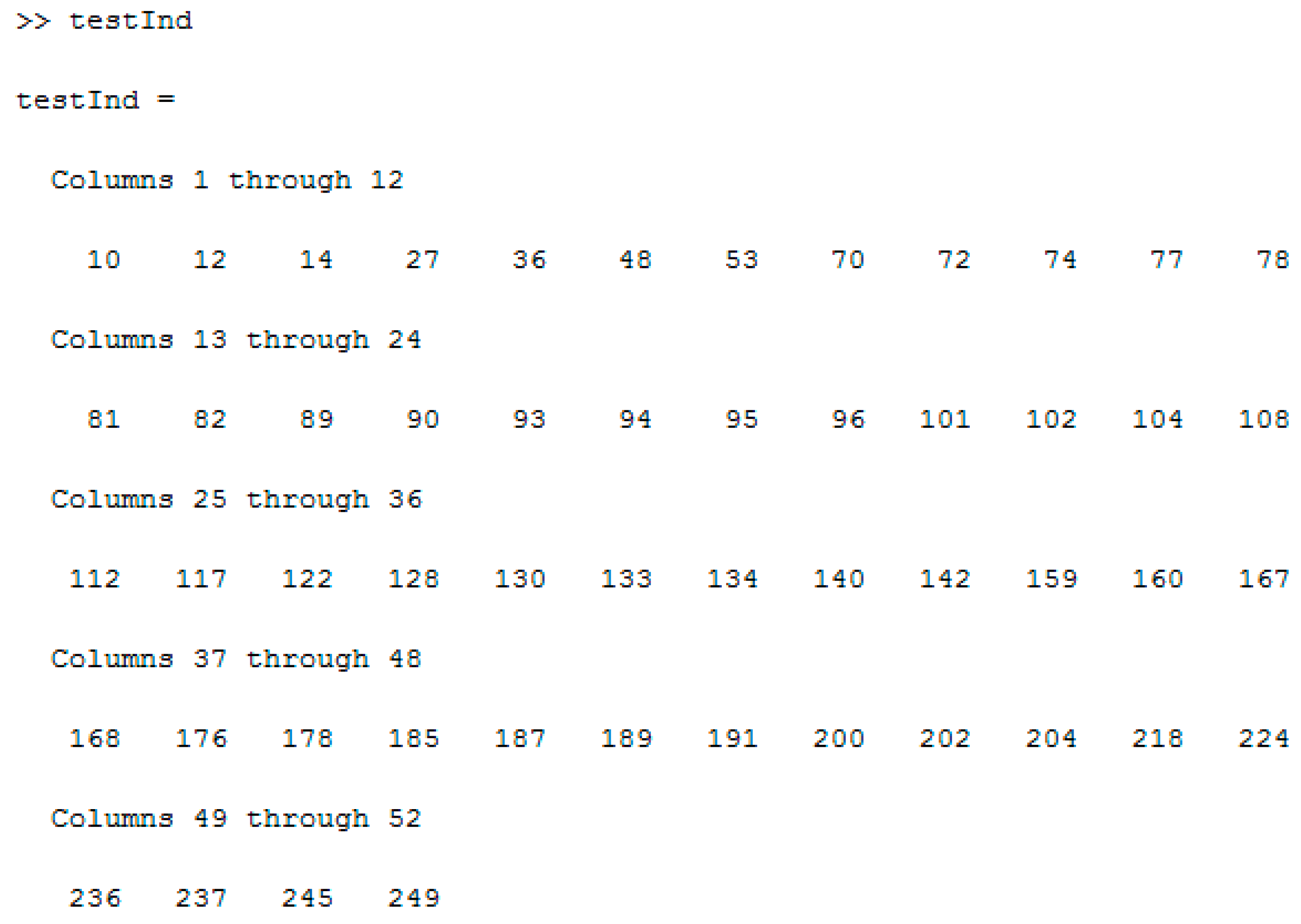
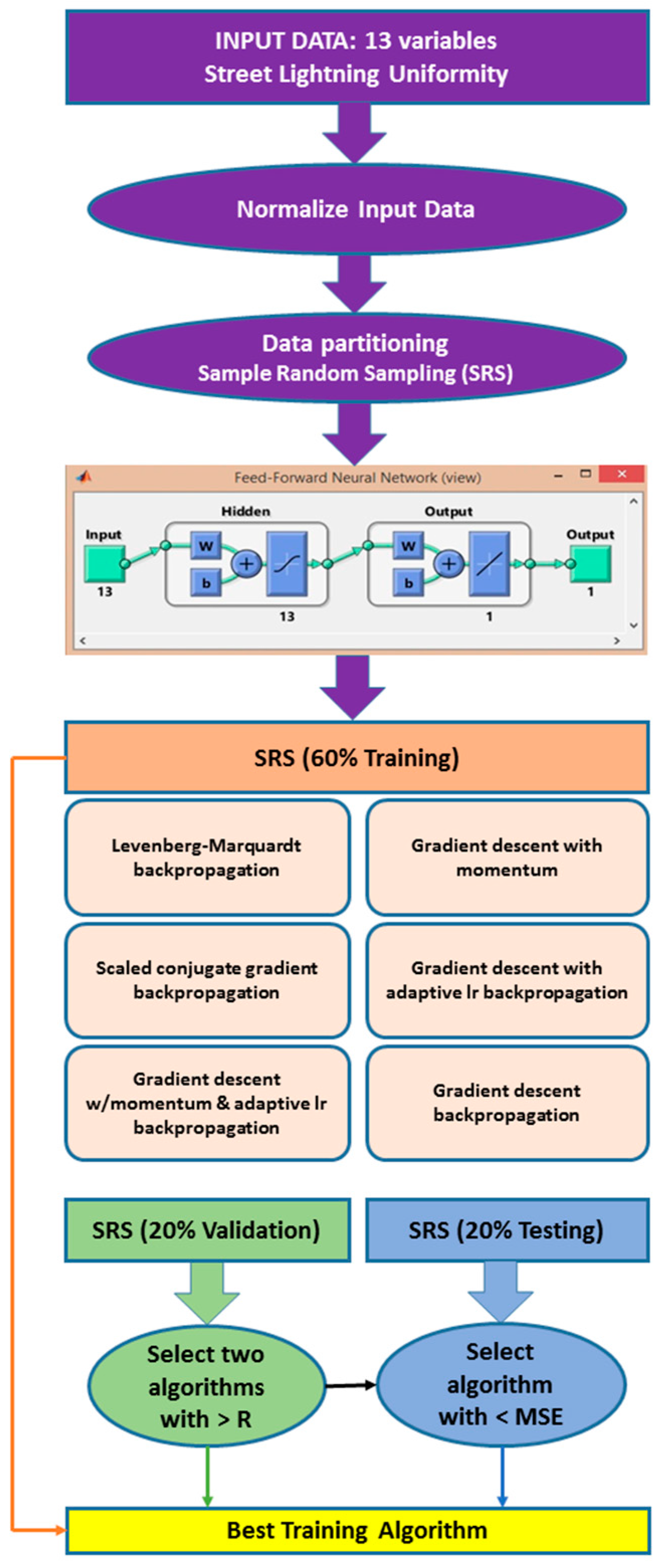
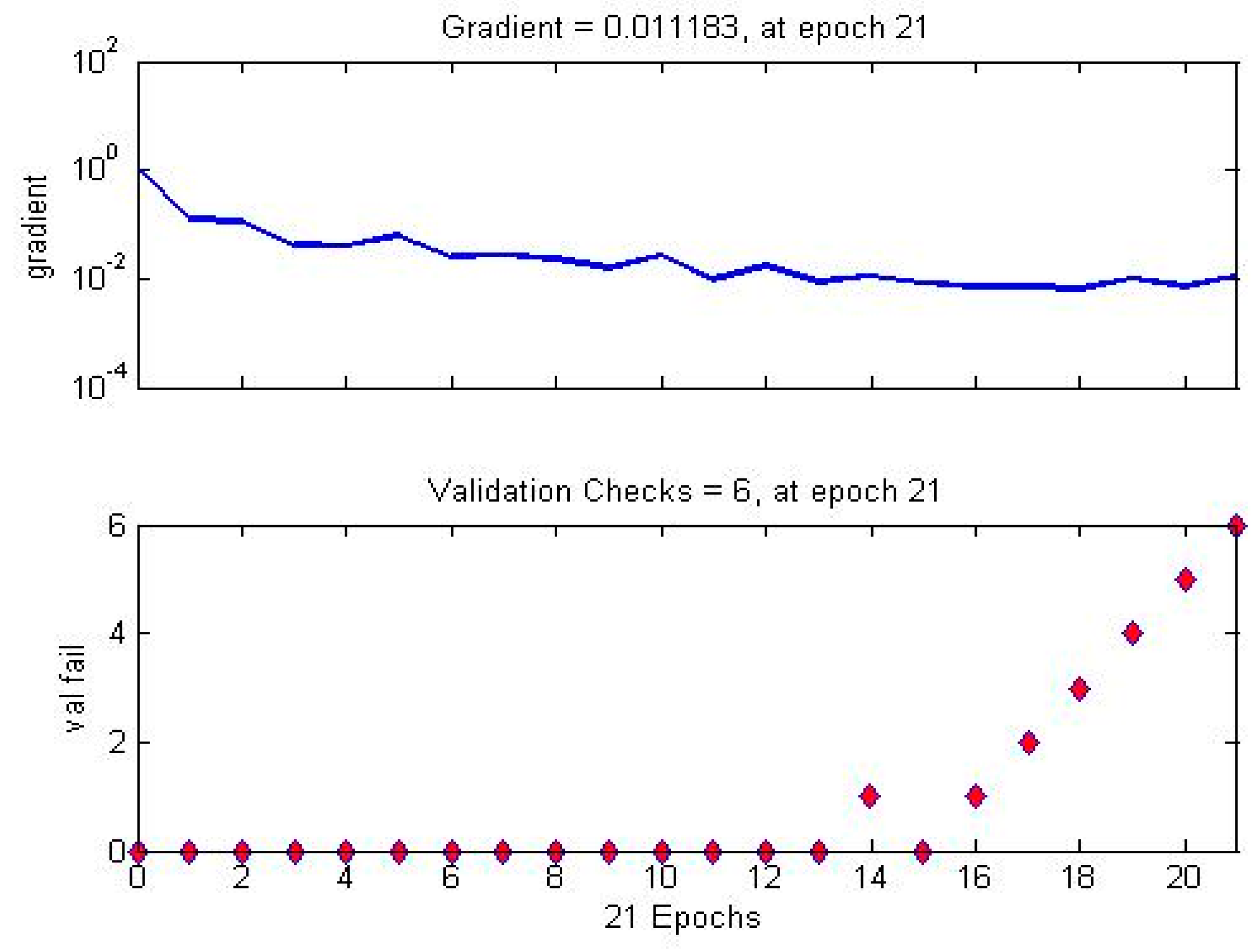
3.8. Validation Process

The validation process of our algorithm consist of selecting the best training algorithm according to the regression parameter and average error obtained during the global process. Figure 4 shows a flow chart of the ANN. Firstly, because thirteen different input variables were used, the data was normalized in order to have the same range for each parameter. Next, a simple random sampling (SRS) partitioning method was selected to select the set of variables for training, validation and testing of the ANN. Note that the same set of data was used to analyze the six training algorithms and by using the same ANN architecture (feed-forward network). For the ANN training, 60% of data was used to analyze the six training algorithms, whereas 20% was used for the validation step and the remaining 20% for the testing step. Finally, our selection criteria was to choose the training algorithm that fulfilled the following rules:
(1)
Select the two algorithms with the highest regression parameters (R) for the training step
(2)
Select the two algorithms with the highest regression parameters (R) for the validation step
(3)
Select the algorithm with the lowest values (MSE) in all the processes.
When an ANN is trained it is wrong to consider only the test process in order to establish the best trained ANN. All the processes should be considered in order to establish the best training algorithm of the network [45,46,47,48,49,50,51,52,53].

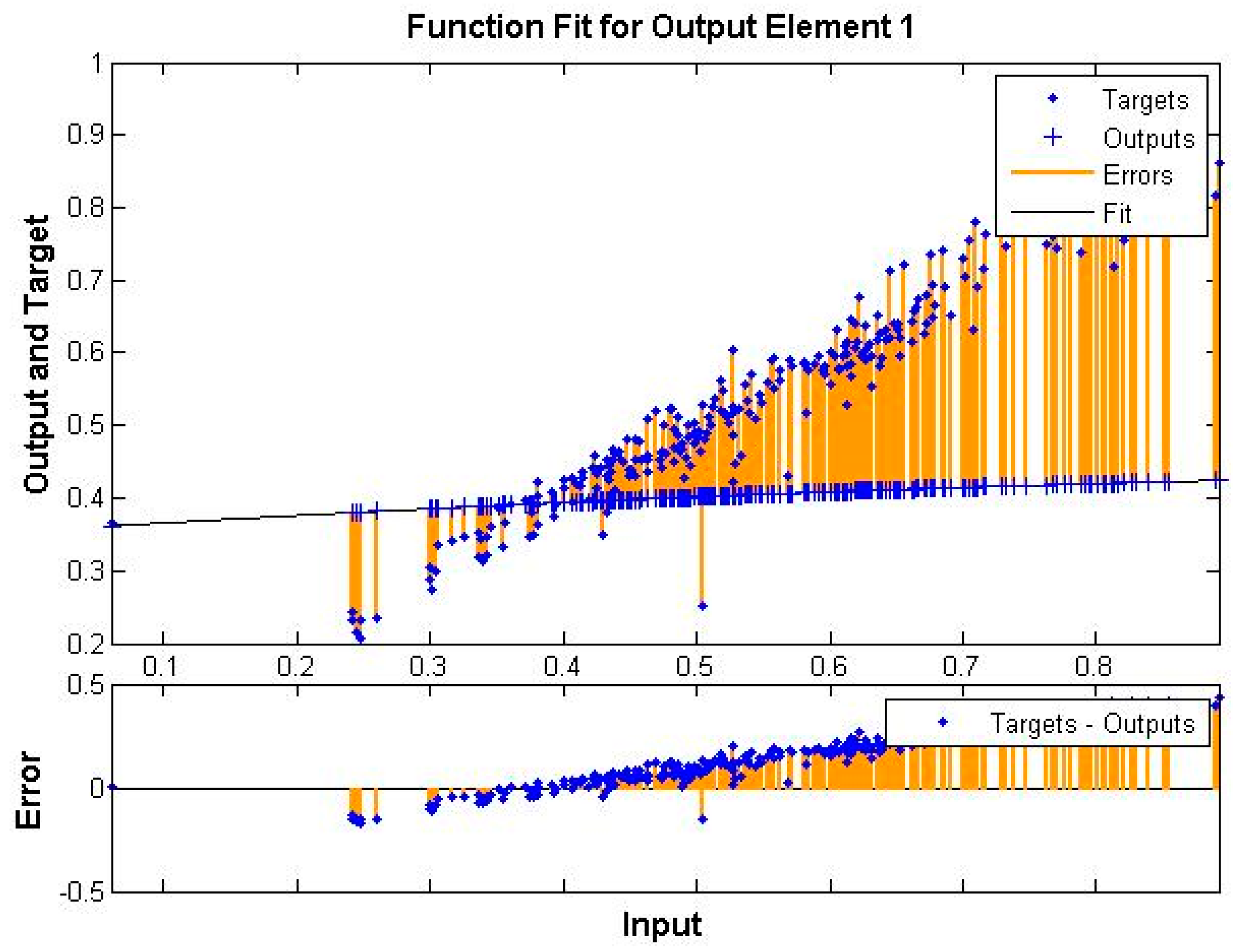
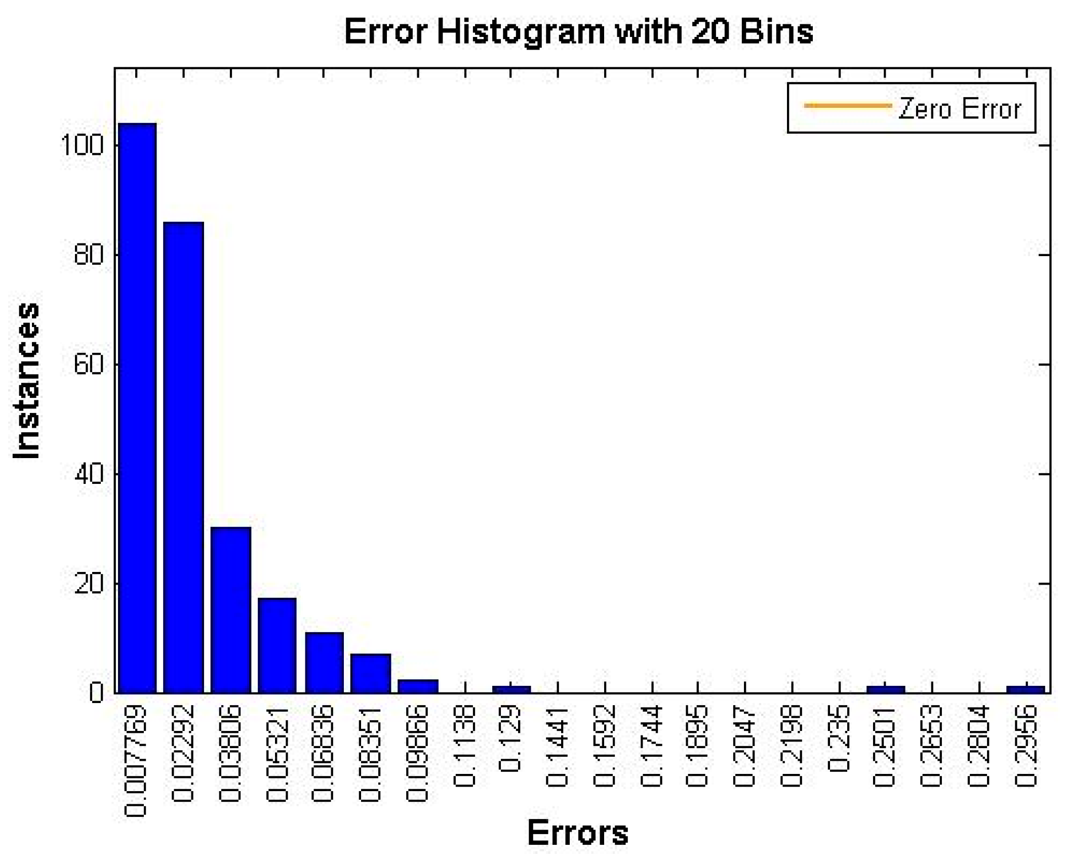
4. Experimental Results and Discussion

This section describes the process followed in the development of the neural network and the experiments performed to select the optimal training algorithm. To do that, the Matlab software (R2015b, Mathworks, Natick, MA, USA) package and its nnstart tool were used. The experiment data consisted on 260 values for street lighting uniformity; all of them matched the specification of the 13 variables of the installation structure (see Table 1).
For learning process, all the data obtained for the development of the ANN was randomly divided into sets of 60% for training (156), 20% for validation (52) and for 20% for testing (52), using a total of 260 patterns of data. For this, we have used the Matlab function dividerand. This function returns the random indexes that allow us to choose the respective data sets according to the sizes specified in the arguments of the function call:
[trainInd, valInd, testInd] = dividerand (260, 0.6, 0.2, 0.2)
In this case, the dividerand function separates the targets into three sets and returns the training references in the trainInd variable, the validation references in the valInd variable and the test references in the testInd variable (Figure 5). We can use this information to create the specific datasets to use in every step of the ANN development (Figure 6).
After the data sets were constructed, we had to create the architecture of the ANN. As discussed previously, a feed-forward neural network was selected to perform the experiments. The ANN consisted in 13 inputs, one for each of the variables of the installation structure, 13 hidden neurons and one output as target for the desired uniformity (Figure 7).
Next, the Matlab utility nntraintool was used to perform the training of the ANN. This tool opens a data manager window, which allows importing, creating, using, and exporting neural networks data experiments. Figure 8 shows an example of the nntraintool when the Scaled Conjugate Gradient training algorithm was used.
Once training is completed, we can use the information provided by nntraintool to analyze the results obtained with every algorithm. First, the performance button plots a graph with the error found in the training step. The performance of the six algorithms in terms of error was compared in the Figure 9. It is possible to check that both the scaled conjugate gradient back-propagation and Levenberg-Marquardt back-propagation algorithms are the closest to the desired output because they present the lowest errors.
Next, for every training algorithm and for every phase (training, validation and testing), information about the mean squared error (MSE) and the regression (R) values was obtained. Table 2 compares the MSE and the R values. The highest regression value for the training process) was obtained with the gradient descent back-propagation. For the validation process, the highest regression value was obtained using the Levenberg-Marquardt back-propagation (0.899) method and for the test process, it was obtained using the gradient descent back-propagation (0.812). Although the Levenberg-Marquardt back-propagation training algorithm presents the lowest MSE values in all the processes, and according with our validation process (in Section 3.8), we can conclude that the best training algorithm is the Levenberg-Marquardt back-propagation one.
In terms of probability, Figure 10 shows the regression function by comparing the actual output of the neural network with the corresponding desired output target for every training algorithm.
These checks ensure that the best results for the ANN are obtained with the Levenberg-Marquardt back-propagation algorithm, so estimations are very close to the desired output. Overall results after the training, validation and testing phases of the ANN are shown in Figure 11, where it can be seen that the ANN fits the best value after 15 epochs.
As it can be seen in the performance plot, the MSE of the ANN has decreased with the number of epochs. The ANN was well trained so presents a very low MSE at the end of the training phase. Because the MSE, that is, the distance between the model’s estimate of the test values and the actual test value, is very small (close to zero), it means that the desired outputs and the ANN’s outputs for the training set have become very close to each other.
Next, Figure 12 shows the evolution of the gradient in the search of the minimum of the cost function (uniformity) versus the number of validation checks. The magnitude of the gradient and the number of validation checks are used to terminate the training. The gradient will become very small as the training reaches a minimum of its performance. The number of validation checks represents the number of successive iterations that the validation performance fails to decrease.
Figure 13 shows the evolution of the error (as target—output) while the ANN is trained to fit the desired value for the cost function.
Next, Figure 14 shows a histogram with the evolution of the error depending of the number of instances used in the ANN training phase. The histogram can give us an indication of outliers, which are data points where the fit is significantly worse than for the majority of the data. In this case, as the number of instances increases, the error decreases.
Finally, in the Figure 15, the learning curve of our neural network can be compared with the best training algorithm. This graph shows a regression analysis between the response of the network and the desired objectives. The value of R indicates the correlation coefficient between outputs and objectives. This value corresponds with the R-value shown in Table 2 for the Levenberg-Marquardt back-propagation training function in the validation step. The output tracks the targets very well for validation, and the R-value is over 0.96, that is, the network response is satisfactory.
All this is a measure of how well the output is adapted to the targets. Thus, if R equals 1 means there is perfect correlation. Then, to evaluate the algorithms, we compared the error obtained after analyzing the samples collected in the testing phase.

5. Conclusions

A new algorithm that is able to find the best installation configuration with the purpose of obtaining the overall illuminance uniformity was presented. The goal is to improve the quality of street lighting systems. A feed-forward back-propagation neural network can be used as a highly effective tool for analyzing overall uniformity in outdoor lighting systems with an appropriate combination of learning, transfer and training functions. The ANNs were simulated and trained with all the above-mentioned algorithms using avtraining dataset. In the proposed work after the experiments, we found that, on average, the algorithm that best minimizes the error is the Levenberg-Marquardt back-propagation one, which approximates the desired output of the training pattern. This kind of algorithms will help lighting professionals optimize the quality of street lighting installations and reduce their electricity consumption.

Author Contributions

Ana Castillo-Martinez and José Manuel Gómez-Pulido have contributed developing ideas about energy efficiency. Antonio del Corte-Valiente and José Luis Castillo-Sequera have obtained the training data and used Matlab for the ANNs. Jose-Maria Gutierrez-Martinez validated the results obtained with the ANNs. All the authors were involved in preparing the manuscript.

Conflicts of Interest

The authors declare no conflict of interest.

References

  1. Lorenc, T.; Petticrew, M.; Whitehead, M.; Neary, D.; Clayton, S.; Wright, K.; Thomson, H.; Cummins, S.; Sowden, A.; Renton, A. Environmental interventions to reduce fear of crime: Systematic review of effectiveness. J. Syst. Rev. 2013, 2. [Google Scholar] [CrossRef] [PubMed]
  2. Space, D. Crime Prevention through Environmental Design; Mac: New York, NY, USA, 1972. [Google Scholar]
  3. Reusel, K.V. A look ahead at energy-efficient electricity applications in a modern world. In Proceedings of the European Conference on Thermoelectrics, Bergen, Norway, 16–20 June 2008.
  4. Equipment Energy Efficiency (E3) Program. Street Lighting Strategy. Available online: http://www.energyrating.gov.au/wp-content/uploads/Energy_Rating_Documents/Library/Lighting/Street_Lighting/Draft-streetlight-Strategy.pdf (accessed on 18 October 2016).
  5. Herranz, C. Interview with Alfonso Beltrán García-Echaniz, managing director of the Institute for Diversification and Energy Saving (IDAE). J. Phys. Soc. 2011, 21, 26–29. [Google Scholar]
  6. Dully, M. Traffic Safety Evaluation of Future Road Lighting Systems. Master’s Thesis, Linköping University, Linköping, Sweden, 2013. [Google Scholar]
  7. Coetzer, R.C.; Hancke, G.P. Eye detection for a real-time vehicle driver fatigue monitoring system. In Proceedings of the Intelligent Vehicles Symposium (IV), Baden-Baden, Germany, 5–9 June 2011.
  8. Güler, Ö.; Onaygil, S. A new criterion for road lighting: Average visibility level uniformity. J. Light Vis. Environ. 2003, 27, 39–46. [Google Scholar] [CrossRef]
  9. Matout, N. Estimation of the Influence of Artificial Roadway Lighting on Road Collision Frequency. Ph.D. Thesis, Concordia University, Montreal, QC, Canada, 2013. [Google Scholar]
  10. Halonen, L.G. Intelligent Road Lighting Control Systems; Report 50; Helsinki University of Technology: Espoo, Finland, 2008. [Google Scholar]
  11. Royal Decree 1890/2008 (2008), 14th November, by Approving Energetic Efficiency. Regulation in Outdoor Lighting Installations and Their Complementary Instructions EA-01 and EA-07. Available online: https://www.boe. es/boe/dias/2008/11/19/pdfs/A45988-46057. pdf (accessed on 5 January 2015).
  12. Fournier, F.; Cassarly, W.J.; Rolland, J.P. Method to improve spatial uniformity with lightpipes. Opt. Lett. 2008, 33, 1165–1167. [Google Scholar] [CrossRef] [PubMed]
  13. Yang, H.; Bergmans, J.W.; Schenk, T.C.; Linnartz, J.P.; Rietman, R. Uniform illumination rendering using an array of LEDs: A signal processing perspective. IEEE Trans. Signal Process. 2009, 57, 1044–1057. [Google Scholar] [CrossRef]
  14. Daliakopoulos, I.N.; Coulibaly, P.; Tsanis, I.K. Groundwater level forecasting using artificial neural networks. J. Hydrol. 2005, 309, 229–240. [Google Scholar] [CrossRef]
  15. Sędziwy, A.; Kozień-Woźniak, M. Computational support for optimizing street lighting design. J. Complex Syst. Dependabil. 2012, 170, 241–255. [Google Scholar]
  16. Jackett, M.; Frith, W. Quantifying the impact of road lighting on road safety—A New Zealand study. IATSS Res. 2013, 36, 139–145. [Google Scholar] [CrossRef]
  17. Lighting against Crime. A Guide for Crime Reduction Professionals. Available online: http://www.securedbydesign.com/ pdfs/110107_LightingAgainstCrime.pdf (accessed on 18 October 2016).
  18. Mara, K.; Underwood, P.; Pasierb, B.P.; McColgan, M.; Morante, P. Street Lighting Best Practices; Hiline Enegineering: Richland, WA, USA, 2005. [Google Scholar]
  19. Fisher, A. A Review of Street Lighting in Relation to Road Safety; Australian Government Publishing Service: Canberra, Australia, 1971. [Google Scholar]
  20. Anderson, N.H. Empirical Directions in Design and Analysis; Erlbaum: Mahwah, NJ, USA, 2001. [Google Scholar]
  21. McLeod, I. Simple random sampling. In Encyclopedia of Statistical Sciences; Kotz, S., Johnson, N.L., Eds.; Wiley: New York, NY, USA, 1988; Volume 8, pp. 478–479. [Google Scholar]
  22. Schaeffer, R.L.; Ott, R.L.; Mendenhall, W. Elementary Survey Sampling, 6th ed.; Thompson Learning: Belmont, CA, USA, 2006. [Google Scholar]
  23. Pizzuti, S.; Annunziato, M.; Moretti, F. Smart street lighting management. Energy Effic. 2013, 6, 607–616. [Google Scholar] [CrossRef]
  24. Benardos, P.G.; Vosniakos, G.C. Optimizing feedforward artificial neural network architecture. Eng. Appl. Artif. Intell. 2007, 20, 365–382. [Google Scholar] [CrossRef]
  25. Cybenko, G. Approximation by superpositions of a sigmoidal function. Math. Control Signals Syst. 1989, 2, 303–314. [Google Scholar] [CrossRef]
  26. Hornik, K.; Stinchcombe, M.; White, H. Multilayer feedforward networks are universal approximators. Neural Netw. 1989, 2, 359–366. [Google Scholar] [CrossRef]
  27. Barron, A.R. A comment on “Neural networks: A review from a statistical perspective”. Stat. Sci. 1994, 9, 33–35. [Google Scholar] [CrossRef]
  28. Lippmann, R.P. An introduction to computing with neural nets. IEEE ASSP Mag. 1987, 4, 4–22. [Google Scholar] [CrossRef]
  29. Cybenko, G. Continuous Valued Neural Networks with Two Hidden Layers are Sufficient; Technical Report; Tuft University: Medford, MA, USA, 1988. [Google Scholar]
  30. Lapedes, A.; Farber, R. How neural nets work. In Neural Information Processing Systems; Anderson, D.Z., Ed.; American Institute of Physics: New York, NY, USA, 1988; pp. 442–456. [Google Scholar]
  31. Wong, F.S. Time series forecasting using back-propagation neural networks. Neurocomputing 1991, 2, 147–159. [Google Scholar] [CrossRef]
  32. Tang, Z.; Fishwick, P.A. Feedforward neural nets as models for time series forecasting. ORSA J. Comput. 1993, 5, 374–385. [Google Scholar] [CrossRef]
  33. Kang, S. An Investigation of the Use of Feedforward Neural Networks for Forecasting. Ph.D. Thesis, Kent State University, Kent, OH, USA, 1991. [Google Scholar]
  34. De Groot, C.; Wurtz, D. Analysis of univariate time series with connectionist nets: A case study of two classical examples. Neurocomputing 1991, 3, 177–192. [Google Scholar] [CrossRef]
  35. Levenberg, K. A method for the solution of certain non-linear problems in least squares. Q. Appl. Math. 1944, 2, 164–168. [Google Scholar] [CrossRef]
  36. Marquardt, D.W. An algorithm for the least-squares estimation of nonlinear parameters. SIAM J. Appl. Math. 1963, 11, 431–441. [Google Scholar] [CrossRef]
  37. Kaj Madsen, Hans Bruun Nielsen, Ole Tingleff Methods for Non-Linear Least Squares Problems (2nd ed.). Informatics and Mathematical Modelling, Technical University of Denmark, DTU. Available online: http://www2.imm.dtu.dk/pubdb/views/edoc_download.php/3215/pdf/imm3215.pdf (accessed on 25 January 2017).
  38. Lourakis, M.L.; Argyros, A.A. Is levenberg-marquardt the most efficient optimization algorithm for implementing bundle adjustment? In Proceedings of the Tenth IEEE International Conference on Computer Vision, Marseille, France, 12–18 October 2005.
  39. Wilamowski, B.M.; Iplikci, S.; Kaynak, O.; Efe, M.O. An algorithm for fast convergence in training neural networks. In Proceedings of the International Joint Conference on Neural Networks, Washington, DC, USA, 15–19 July2001.
  40. Møller, M.F. A scaled conjugate gradient algorithm for fast supervised learning. Neural Netw. 1993, 6, 525–533. [Google Scholar] [CrossRef]
  41. Gopalakrishnan, K. Effect of training algorithms on neural networks aided pavement diagnosis. Int. J. Eng. Sci. Technol. 2010, 2, 83–92. [Google Scholar] [CrossRef]
  42. Beale, M.; Hagan, M.; Demut, H. Neural Network Toolbox User’s Guide; Mathworks: Natick, MA, USA, 2010. [Google Scholar]
  43. Pramanik, N.; Panda, R.K. Application of neural network and adaptive neurofuzzy inference systems for river flow prediction. Hydrol. Sci. J. 2009, 54, 247–260. [Google Scholar] [CrossRef]
  44. Makarynskyy, O. Improving wave predictions with artificial neural networks. Ocean Eng. 2004, 31, 709–724. [Google Scholar] [CrossRef]
  45. Mba, L.; Meukam, P.; Kemajou, A. Application of artificial neural network for predicting hourly indoor air temperature and relative humidity in modern building in humid region. Energy Build. 2016, 121, 32–42. [Google Scholar] [CrossRef]
  46. Chae, Y.T.; Horesh, R.; Hwang, Y.; Lee, Y.M. Artificial neural network model for forecasting sub-hourly electricity usage in commercial buildings. Energy Build. 2016, 111, 184–194. [Google Scholar] [CrossRef]
  47. Ji, Y.; Xu, P.; Duan, P.; Lu, X. Estimating hourly cooling load in commercial buildings using a thermal network model and electricity submetering data. Appl. Energy 2016, 169, 309–323. [Google Scholar] [CrossRef]
  48. Moon, J.W.; Chung, S.K. Development of a thermal control algorithm using artificial neural network models for improved thermal comfort and energy efficiency in accommodation buildings. Appl. Therm. Eng. 2016, 103, 1135–1144. [Google Scholar] [CrossRef]
  49. Kariminia, S.; Motamedi, S.; Shamshirband, S.; Piri, J.; Mohammadi, K.; Hashim, R.; Roy, C.; Petković, D.; Bonakdari, H. Modelling thermal comfort of visitors at urban squares in hot and arid climate using NN-ARX soft computing method. Theor. Appl. Climatol. 2016, 124, 991–1004. [Google Scholar] [CrossRef]
  50. Papantoniou, S.; Kolokotsa, D. Prediction of outdoor air temperature using neural networks: Application in 4 European cities. Energy Build. 2016, 114, 72–79. [Google Scholar] [CrossRef]
  51. Şahin, M.; Oğuz, Y.; Büyüktümtürk, F. ANN-based estimation of time-dependent energy loss in lighting systems. Energy Build. 2016, 116, 455–467. [Google Scholar] [CrossRef]
  52. Kim, W.; Jeon, Y.; Kim, Y. Simulation-based optimization of an integrated daylighting and HVAC system using the design of experiments method. Appl. Energy 2016, 162, 666–674. [Google Scholar] [CrossRef]
  53. Romero, V.P.; Maffei, L.; Brambilla, G.; Ciaburro, G. Modelling the soundscape quality of urban waterfronts by artificial neural networks. Appl. Acoust. 2016, 111, 121–128. [Google Scholar] [CrossRef]
Figure 1. A DIALux street lighting simulation.
Energies 10 00175 g001
Figure 2. Structure of a feed-forward network.
Energies 10 00175 g002
Figure 3. Three sigmoid (for c = 1, c = 2 and c = 3).
Energies 10 00175 g003
Figure 4. Flowchart of the ANN.
Energies 10 00175 g004
Figure 5. Data of the ANN randomly divided into sets.
Energies 10 00175 g005
Figure 6. Indexes returned by the dividerand function.
Energies 10 00175 g006
Figure 7. Architecture of the ANN.
Energies 10 00175 g007
Figure 8. Matlab nntraintool.
Energies 10 00175 g008
Figure 9. ANN error comparison.
Energies 10 00175 g009
Figure 10. ANN probability for normal distribution.
Energies 10 00175 g010
Figure 11. ANN best validation performance.
Energies 10 00175 g011
Figure 12. ANN gradient evolution.
Energies 10 00175 g012
Figure 13. ANN cost function adjustment.
Energies 10 00175 g013
Figure 14. Histogram of error evolution.
Energies 10 00175 g014
Figure 15. Learning curve of the neural network.
Energies 10 00175 g015
Table 1. ANN input pattern variables.
Variable NameVariable Description
Type of lampMercury Vapor
High Pressure Sodium Vapor
Low Pressure Sodium Vapor
Metal Halide
LED
Luminaire arrangementUnilateral
Paired
Quincunx
Power of the lampPower consumed divided by the time it takes to consume [w]
Width of the lampPhysical dimension of the lamp [cm]
InterdistanceDistance between two luminaires [m]
Spacing between luminaire and roadDistance between the lights and the road [m]
Mounting heightData Lamp height [m]
Arm lengthLength of the arm supporting the lamp [m]
Tilt armTilt arm supporting the lamp [degrees]
System fluxMeasure of perceived light output [lumen]
Lamp fluxPower emitted by a light source as visible radiation [lumen]
Colour temperatureTemperature of an ideal black-body radiator that radiates light of comparable hue to the light source [°K]
Luminaire powerPower of the complete lighting unit [w]
Table 2. ANN input pattern variables.
Training MethodsStepMSER
Levenberg-Marquardt back-propagationTraining0.01230.6644
Validation0.00950.8997
Testing0.0516−0.0531
Scaled conjugate gradient back-propagationTraining1.66270.1063
Validation0.37120.8983
Testing0.01460.6128
Gradient descent with momentumTraining0.5760−0.3032
Validation0.0503−0.8773
Testing0.0535−0.0212
Gradient descent with adaptive lr back-propagationTraining4.36410.3517
Validation4.06300.1115
Testing0.12680.3491
Gradient descent w/momentum & adaptive lr back-propagationTraining6.0454−0.0046
Validation0.03050.3640
Testing0.2339−0.3598
Gradient descent back-propagationTraining0.01550.6747
Validation0.00540.8820
Testing0.37530.8123

