Article

Risk-Based Probabilistic Voltage Stability Assessment in Uncertain Power System

School of Electrical and Electronic Engineering, Huazhong University of Science and Technology, 1037 Luoyu Road, Wuhan 430074, China
*
Author to whom correspondence should be addressed.
Energies 2017, 10(2), 180; https://doi.org/10.3390/en10020180
Submission received: 28 October 2016 / Revised: 19 January 2017 / Accepted: 23 January 2017 / Published: 5 February 2017

Abstract

:
The risk-based assessment is a new approach to the voltage stability assessment in power systems. Under several uncertainties, the security risk of static voltage stability with the consideration of wind power can be evaluated. In this paper, we first build a probabilistic forecast model for wind power generation based on real historical data. Furthermore, we propose a new probability voltage stability approach based on Conditional Value-at-Risk (CVaR) and Quasi-Monte Carlo (QMC) simulation. The QMC simulation is used to speed up Monte Carlo (MC) simulation by improving the sampling technique. Our CVaR-based model reveals critical characteristics of static voltage stability. The distribution of the local voltage stability margin, which considers the security risk at a forecast operating time interval, is estimated to evaluate the probability voltage stability. Tested on the modified IEEE New England 39-bus system and the IEEE 118-bus system, results from the proposal are compared against the result of the conventional proposal. The effectiveness and advantages of the proposed method are demonstrated by the test results.

1. Introduction

With the rapid growth of power demand, modern power grids have been changing incredibly throughout the world. Despite the sustainable features, wind power generation introduces uncertainties to the entire power system. Additionally, load forecasting errors with respect to the change of operating conditions also contribute to the system uncertainties. Therefore, the risks of bearing these uncertainties during operating states must be quantified and fully investigated. The security of the voltage stability problem considered in this paper is motivated by the increasing presence of stochastic elements in the power system as a result of integrating intermittent renewables at both the wholesale and retail levels. The surge of solar power integration in recent years, for example, has fundamentally changed the overall net load characteristics. In some areas, the traditional load profile is being transformed to the so-called “duck curve” profile where a steep down-ramp during the hours when a large amount of solar power is injected into the network is followed by a steeper up-ramp when the solar power drops sharply in the late afternoon and early evening hours.
While the duck curve phenomenon represents an average net load behavior, it is the highly stochastic and spatial-temporal-dependent ramp event that presents difficult operational challenges to system operators. For this reason, power system voltage stability is one of major topics of concern for secure operation of transmission networks. It is defined as the ability of a power system to maintain load voltage magnitudes after disturbances [1]. The static method is widely analyzed for voltage stability assessment when large demand and limited network expansion occur. The relationship between transmitted power and receiving end voltage (PV) curve is one of the powerful tools for stability analysis [2]. The work in [3]
provides an index that accounts for both the future uncertainties on the system and the consequences associated with voltage collapse and violation of limits. Besides, Reference [4] proposes an on-line voltage security method based on wide-area measurements and a decision tree. While the operating point reaches the critical voltage collapse point, the system may lose controllability and face a series of cascading outages problem. Furthermore, due to the load fluctuation and intermittent energy behavior, it is hard to predict the system operational status. The voltage stability analysis should consider how to accurately express the system’s risks.
Probabilistic risk-based approaches have been adopted for not only power system planning, but also the security assessment for the last decades [5,6,7]. The work in [8] provides an AFTER (A Framework for electrical power sysTem vulnerability identification, dEfense and Restoration) in-depth risk assessment tool to deal with extreme events for static security assessment, such as threats, vulnerability, contingency and impact. Otherwise, Reference [9] introduces a transmission line overload risk index for measuring the security level of wind integrated power systems considering the wind and load-power generation correlation. Besides, a fuzzy risk assessment of small-disturbance stability has been proposed in [10] to handle the rotor angle instability. The literature for voltage risk assessment is rather limited. In order to quantitatively evaluate the voltage stability risk, Reference [11] provides a stability index for determining the bifurcation point of the power system. The voltage instability probability is calculated based on a joint distribution for the entire system [12,13]. The work in [14] addresses the voltage stability topic, including unstable states caused by modeling resolvability and loss of controllability. The risk of high distribution generation penetration in a low-voltage secondary distribution network affecting voltage stability is analyzed in [15]. The work in [16] proposes a set of risk indices to tell the weak lines and buses of the system, which can bring in static voltage instability, and the author also provides an assessment technique to calculate them. Furthermore, risk can also be used for the application of security-constrained optimal power flow to describe the system health [17,18].
The stochastic nature of the system uncertainties requires the probabilistic approach to cope with them. These techniques could be classified under three main categories: cumulant method, point estimate method and Monte Carlo (MC) simulation. The cumulant method is widely used for solving probabilistic power flow [19,20,21], which is computationally effective, but requires some mathematical assumptions in order to simplify the problem. The cumulant method combined with the Gram–Charlier expansion is used to estimate the output distribution [20,22]. Later, the method of cumulants and the von Mises function is developed to deal with discrete distributions [21]. Furthermore, point estimate methods provide an approximate statistical description of the output random variables with less computational burden [8,9,23]. The Monte Carlo simulation is widely used as the benchmark method for the reason that circuit size, simulation time, etc., often make Monte Carlo analysis time expensive [24]. In this paper, the Quasi-Monte Carlo (QMC) simulation is made to accelerate the speed of Monte Carlo simulation by improving the technique of sample generation.
Although researchers have made great efforts, these probabilistic risk-based methods are not appropriate enough for large wind power-penetrated system, because these indices cannot reflect the tail risk of the voltage static loss. Furthermore, the randomness and violation are not considered in their forecast model. Hence, a risk-based probabilistic voltage stability assessment is of great value to be learned. As we know, Conditional Value at Risk (CVaR) is used as risk hedging tool in a power system for its advantages of consistency and subadditivity [25,26,27]. Sometimes, it is difficult to calculate CVaR for the reason that it is hard to find an analytical representation of the loss function, which is associate with the distribution of the input random variables [28]. Hence, Monte Carlo simulation is employed to the optimization and calculation of the CVaR to solve this problem. However, the risk-based security assessment is a state-of-the-art method, which will be used in the near future. The Monte Carlo simulation cannot handle the online computation, because of the drawback of the great number of simulations required to obtain convergence [29]. We provide a new voltage stability index based on QMC and CVaR, which reveals important aspects of static voltage stability and is used for the online evaluation of tail risk-based security levels of wind-penetrated power systems.
The paper is organized as follows. In Section 2, the probabilistic model of wind power generation is built by the Gaussian mixture model, whose parameters are obtained according to the Expectation Maximization (EM) algorithm. In Section 3, a security risk index of voltage stability based on CVaR and the PV curve is described. In Section 4, the QMC simulation is adopted to forecast the real-time voltage distribution. In Section 5, two comprehensive case studies are designed, and the corresponding results are analyzed to highlight the advantages of the proposed method.

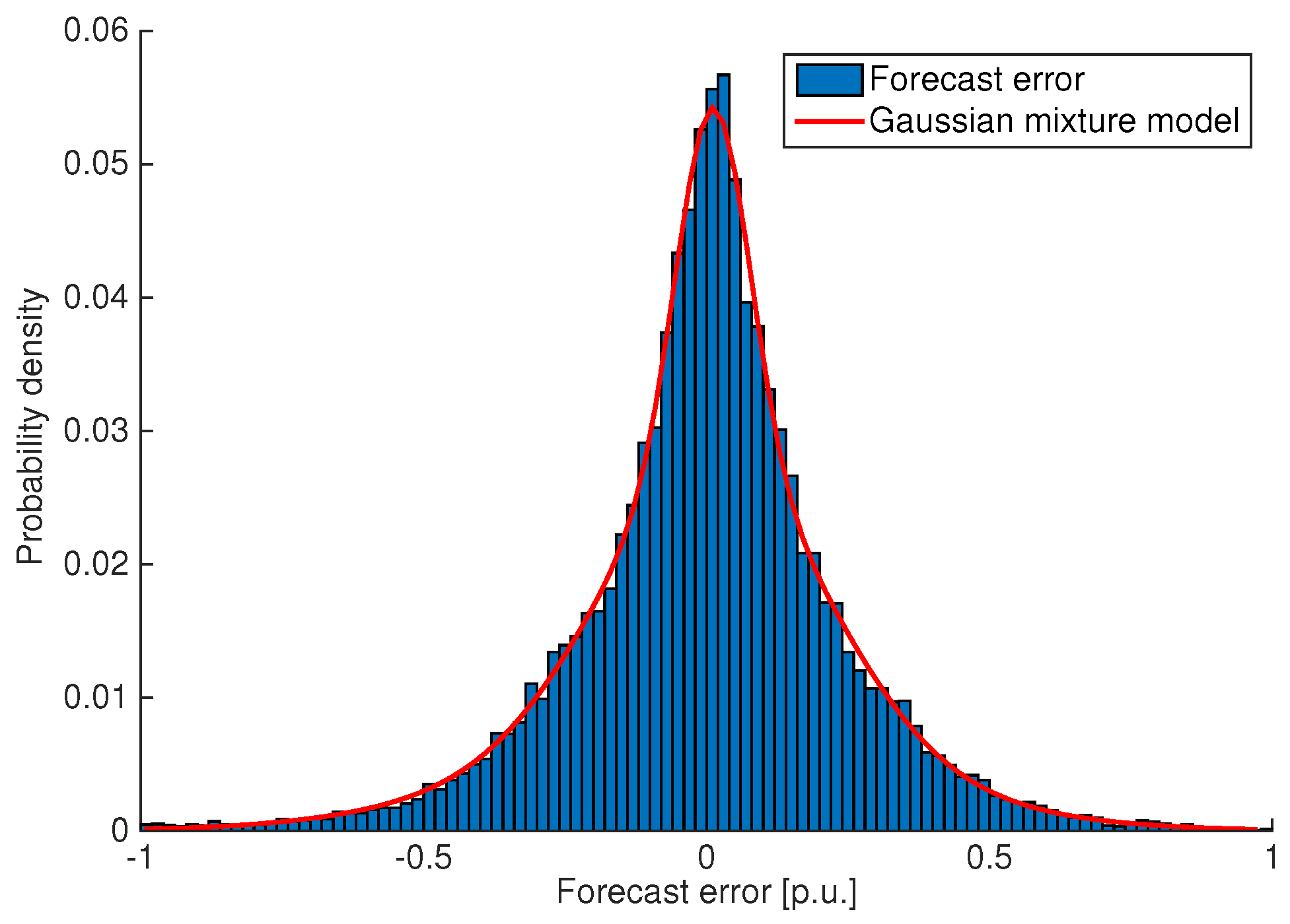
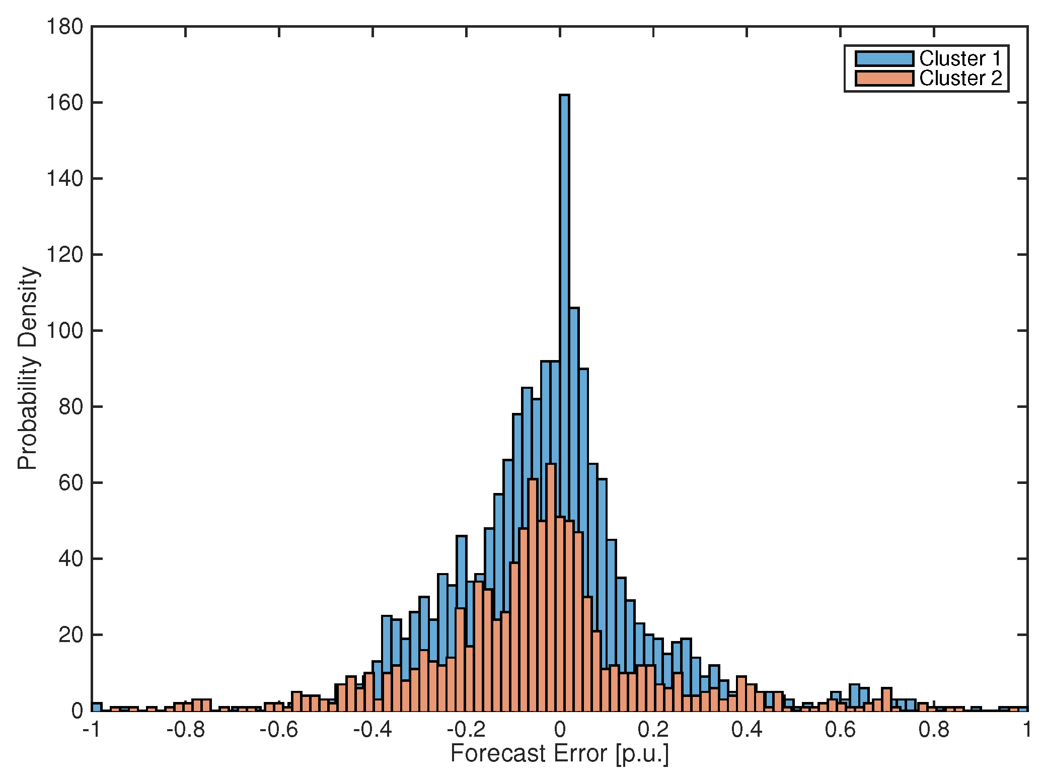
2. Probabilistic Model of Wind Power Generation

Wind power ultra-short-term forecast error is usually assumed to follow a weighted sum of beta distribution. The work in [30] uses the Gaussian mixture distribution to model any non-Gaussian distribution. Furthermore, in order to represent the stochastic power output of wind farms, References [31,32,33] use the Gaussian mixture model to approximate the development for the probability density function (PDF) of wind power generation. The ultra-short-term wind power forecast error distribution, following the Gaussian mixture model at each time interval, had also served in in this paper. Hence, the probability density function of measured wind power can be modeled by a Gaussian mixture model corresponding to different given predicted wind powers. The observed value of the measured wind power is available from the stratified sampling of the wind power scenario tree for a single time interval. According to the observed value, maximum likelihood mixture densities’ parameters can be found via the EM algorithm [34]. In addition, the Stochastic Approximation Expectation Maximization (SAEM) algorithm [35], compared to the EM algorithm, performs better and converges almost surely to a local maximum of the likelihood of the function. In this paper, we obtained 140,160 sampling data from the four years, each of the 15-min wind power historical data on [36], the website of Belgium’s transmission system operator in Europe. The histogram of 15-min forecast error compared with the Gaussian mixture distribution is plotted in Figure 1, which shows that the Gaussian mixture distribution can fit the shape of the forecast error PDF. The PDF and parameters of the Gaussian distribution are calculated by the following equations:
f ( x ) = i = 1 n w i ( x ) 1 2 π σ e ( x μ ) 2 2 σ 2
μ = 1 n i = 1 n e i
σ 2 = 1 n i = 1 n ( e i μ ) 2
where f ( x ) is the PDF of the total forecast error and w i is the weight of the forecast power bin i.

3. Security Risk Evaluation of Voltage Stability Issues

IEEE defines voltage collapse as the process by which voltage instability leads to the loss of voltage in a significant part of the power system. Voltage stability is a complex phenomenon that involves many power system components at once. As mentioned in [37], the voltage collapses take place on different time scales ranging from seconds to hours: (1) electromechanical transients (e.g., generators, regulators condensers) and power electronics (e.g., SVC (Static Var Compensator) , HVDC (High-Voltage Direct Current) reaching reactive power limits) in seconds; (2) discrete switching devices (e.g., action of tap-changers transformers) acting at tens of seconds; (3) load recovery processes in several minutes. Besides, increasing in loading, line tripping or generator outages are also contributing to the voltage collapses, and the method proposed in this paper captures partially of such a complex phenomenon in minutes time scales.
Nowadays, it is of high value to evaluate the safety distance from a normal operational status to a process of cascading trip incident as typical centralized wind farms are integrated. However, the operational status will be estimated to be a probability distribution, instead of a determined point, in the near future when considering the wind uncertainties. In this section, a new index of the risk-based voltage stability margin has been proposed for security risk evaluation of voltage stability analysis when considering the small probability of a serious event in an uncertain environment.

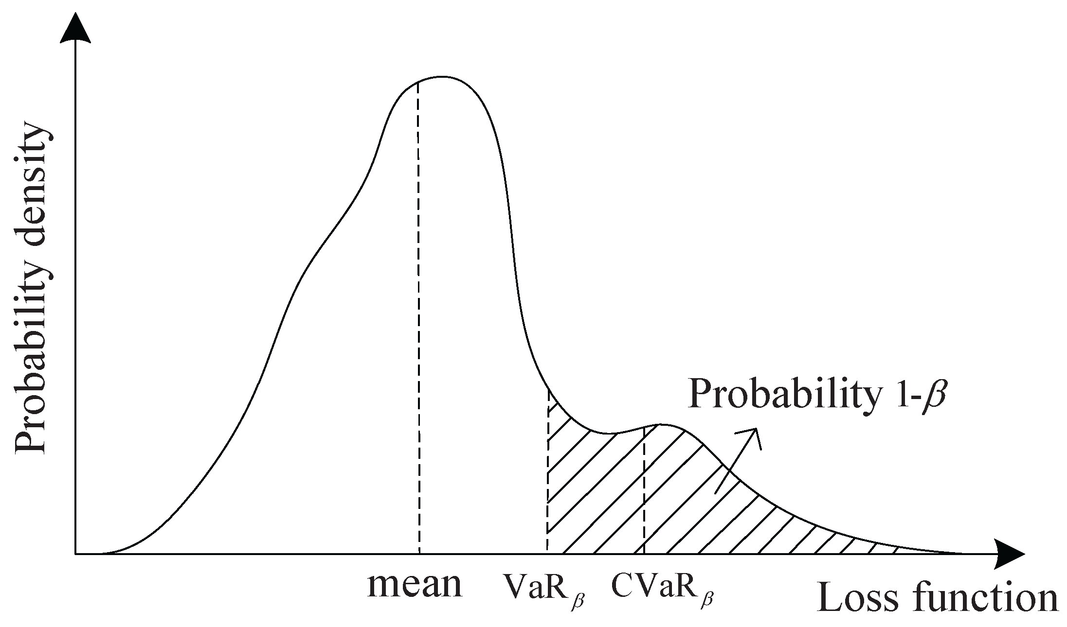
3.1. Definition of Conditional Value at Risk in Security Risk Evaluation

Risk is the potential of gaining or losing something of value [38]. In this paper, risk is associated with ‘security losses’ of the locational voltage of the power system. Risk assessment evaluates the potential voltage stability loss for system operators.
Various methods are used to measure risks. Specifically, CVaR is an index to represent the expected shortfall of the profit distribution at a specified confidence level in finance and banking [39]. Risk measures used for decision making in electricity markets are discussed in [40,41], and the advantages of CVaR are explained. It is considered to be a more consistent measure of risk than Value-at-Risk ( VaR ) [28].
Taking into account the uncertainties associated with electric load and wind power generation integrations, the system may face the risk that the static voltage approaches the voltage collapse point V c p , which is the nose of the PV curve (as shown in Figure 2).
When the system situation reaches the voltage collapse point, a series of uncontrollable cascading events, such as a blackout, may come out step by step. Besides, the voltage collapse value can be obtained by the continues power flow.
The question is how to evaluate the risk of the static security for the power system in an uncertain environment. We define the static voltage stability loss, which is shown as follows:
Ψ ( x , α ) = f ( x , y ) α ρ ( y )   d y
where Ψ ( x , α ) is the cumulative distribution function (CDF) of node voltage stability loss for extreme conditions with respect to demand level x. Furthermore, it is the probability of the relative distance from the node voltage operation point to the collapse point f ( x , y ) without exceeding a threshold α. Besides, ρ ( y ) is the probability density of variance y for f ( x , y ) .
The β- VaR and β- CVaR values for the loss random variable following x and any specified probability level β in ( 0 , 1 ) will be denoted by VaR β ( x ) and CVaR β ( x ) :
VaR β ( x ) = m i n { α R : Ψ ( x , α ) β }
and:
CVaR β ( x ) = E [ x | x V a R β ( x ) ] = 1 1 β f ( x , y ) V a R β ( x ) f ( x , y ) ρ ( y )   d y
In Equation (5), the VaR function, which is the percentile of the loss distribution with confidence level β, is the smallest number, such that Ψ ( x , α ) = β . In Equation (6), the CVaR function is defined as the conditional expected loss associated with x relative to the loss higher than or equal to VaR with probability level β (as shown in Figure 3).
It is difficult to calculate CVaR because it is hard to find an analytical representation of VaR , which has been involved in CVaR ’s definition. Without reference to VaR , a much simpler way of defining CVaR is:
CVaR β ( x ) = F β ( x , α ) = α + 1 ( 1 β ) y R n [ f ( x , y ) α ] + ρ ( y ) d y
where [ ] + = max ( , 0 ) . However, instead of obtaining an analytical expression for the implementation of the approach, it is sufficient to generate random samples y ^ = { y m | y 1 , y 2 , , y M } from the node voltage magnitude distribution via QMC simulation:
CVaR β ( x ) = α + 1 M ( 1 β ) m = 1 M [ f ( x , y m ) α ] +
where M is the number of QMC simulations.

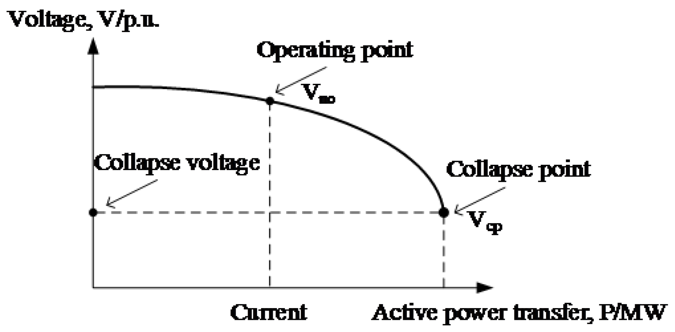
3.2. Index of Voltage Stability Margin Considering the Risk

The steady state relation between injected real power and voltage at a particular bus is described by the PV curve [42] (as shown in Figure 2). It provides sufficient information on the active power margin and voltage magnitude due to small disturbances. The PV curve helps system operators in reliability assessment.
For the purpose of locating the weakest bus of a system, the traditional local voltage stability margin ( V LVSM ) is measured as the relative distance of the voltage magnitude from the operating point ( V n o ) to the voltage collapse point ( V c p , the nose of the PV curve). Furthermore, V LVSM admits a value between zero and one. It is defined as:
V LVSM = V n o V c p V c p
As we consider more and more renewables injected in the power system, the state-of-the-art operational status estimation is deemed to be a probability distribution instead of a deterministic point. Via the results of the probabilistic power flow by the QMC algorithm (Section 4), the probability density functions of the node voltage magnitude can be achieved by modeling the stochastic variation of system uncertainties, such as wind power generation and load fluctuation. We provide a powerful risk-based voltage stability margin index ( V RBVSM ) to measure the security risk of voltage stability loss in the near future. The voltage stability loss is defined as V n o V c p , and V RBVSM is the CVaR β of node voltage stability loss at a specified probability level β. Therefore, the tail risk can be taken into account.
Furthermore, the CVaR-based voltage margin index V RBVSM is a linear sensitive index. It measures the relative distance from the current operational point to the voltage collapse point. This index is of great value for warning about dangers in the proximate future, while it will not change suddenly or sharply until access to the voltage collapse point. It provides ample time for the system operators to make preventive control decisions. Besides, the index is useful for identification of the weakest bus of a system, which helps the system operators focus on these weakest buses, and it can also be used for the application of security-constrained optimal power flow to quantify the system security risk.
Besides V RBVSM , which can be used to measure the risk of voltage stability loss for each local buses, we also provide another voltage stability index, the probabilistic voltage stability margin ( V PVSM % ). As if there is not only one bus that is unstable in the system, the indices can help the system operators to identify the weakest area in the power system for the state-of-art forecast. The n %   V PVSM % is defined as the n % percentage of buses that are voltage stable buses for the near future.
V PVSM % = N s N b %
N s ( i ) = 0 V RBVSM ( i ) 0 1 V RBVSM ( i ) > 0
where N s is the number of voltage stable buses; each indicator function of voltage stable bus N s ( i ) for bus i is calculated in (11); N b is the total number of buses in the power system. They are all estimated for a particular time interval in the near future. Equations (10) and (11) are not the only indices, but help the operators make decisions for preventive control and planning ahead of time.

4. A Quasi-Monte Carlo Simulation for Real-Time Probabilistic Voltage Forecast

In this section, we provide the key theoretical foundation of the probabilistic sampling technique QMC for the real-time static voltage forecast assessment. Instead of generating the pseudo-random samples, the QMC simulation focuses on obtaining a set of low-discrepancy sampling points.

4.1. Quasi Monte Carlo Simulation

Quasi-Monte Carlo methods, using a deterministic set of points from low-discrepancy sequences, aim to outperform the classical Monte Carlo method [43,44,45,46]. The goal for almost all of the MC simulations is to converge to the required accuracy as rapidly as possible, with the least sample simulations. Although pseudo-random sampling points typically used by classical MC are uniformly distributed, geometrically, they suffer from clusters and empty spaces, which are unequally separated over the sampling region. Rather than randomly generating the samples, the QMC tries to select the point set homogeneously equidistantly distributed over the space.
The MC integration error | Q Q n | decreases asymptotically to zeros as convergence rate O ( n 1 2 ) for general integrable f with increasing n [47]. QMC is used to improve on this convergence behavior, which targets the behavior n 1 2 and not the proportionality constant σ ( f ) as the standard variance reduction techniques.
There is another way to analyze the integration error, based on Niederreiter’s development of the concept of discrepancy, which is used to measure the uniformity for finite point sets.
Remark 1
(Discrepancy [44]). Let C s denote the s -dimensional unit cube. For a Jordan measurable set J interval C s and a sequence of N points { x n } in C s , let V o l ( J ) be the volume of J, and let I J ( x ) be the characteristic function of J. Define the n J as the number of points lying inside J,
n J = i = 1 n I J ( x i )
Then, we define the discrepancy as:
D N = sup J C s n J N V o l ( J ) .
If we only look at hyper-rectangles with one corner at zero, J = [ 0 , a ) where a C s , the star discrepancy is defined as:
D N = sup a C s n [ 0 , a ) N V o l ( [ 0 , a ) ) .
Reference [48] shows that for uniform points x i U [ 0 , 1 ) s , the star discrepancy for classical MC is D N = O ( ( l o g l o g N N ) 1 2 ) . However, QMC performs using the samples generated from a deterministic sequence; the low-discrepancy sequence, which has been constructed with star discrepancy bound D N = O ( ( l o g N ) s N ) , yielding a convergence rate of O ( ( l o g N ) s N ) , shows the surprising attribute of asymptotically superior discrepancy, in comparison with the pseudo-random sequence used by classical MC.
Finally, Koksma-Hlawka gives the answer to the question of the relationship of the integration error in MC and the discrepancy of a point set.
Theorem 1
(Koksma-Hlawka [44]). If function f has bounded variation in the sense of Hardy and Krause, then the Monte Carlo error is bounded as follows.
ε ( f ) = | Q Q n | V ( f ) D N *
where V ( f ) = 0 1 | d f | is the variation of f and D N * is the star discrepancy of the sequence { x n } .
By Theorem 1, the Koksma-Hlawka inequality function guides us to search for effective point sets and sequences by making precise the role of star discrepancy. It is particularly attractive because using the points with lower star discrepancy D N might reduce the integration error. Obviously, we see the terrific possibility of linear ( N 1 ) convergence of QMC integration error, instead of the slow ( N 0.5 ) MC integration error [24].
In the field of computational finance, QMC has had widespread success and obvious application [43]. Besides, References [24,49] handle it for the research of statistical static timing analysis, small signal stability analysis and other engineering problems. All of the results show significant gains over classical MC. In this paper, we will try to use it for the calculation of probabilistic power flow.

4.2. The Formulation of the Real-Time Voltage Forecast Problem

In an uncertain environment, with stochastic and intermittent variables injected into the power system, the forecast of node voltage magnitude is not truly deterministic. Most quantities of practical interest present it as probability distributions. Hence, the QMC simulation technique is a state-of-the-art prediction strategy for probabilistic voltage forecast analysis.
The real-time statistic voltage and its posterior probability mass function at time T forecast from initial time t can be obtained by the probabilistic power flow, which is defined as,
p T | t ( j ) = j 1 { V ( j ) = V i ( T ) } M
where j is the number of buses, V i ( T ) is the discrete value of voltage that may occur at time T and M is the number of QMC runs. The indicator function 1 { } is set to be one, while the voltage at bus j is V i ( T ) .
The computation of the above conditional probabilities depends on a probabilistic model of the power injections, such as wind power generation W { w 1 , w 2 , , w m } and load D { d 1 , d 2 , , d m } . The relationships of voltage state V i , W and D are described in Equation (17).
V i = f i ( d 1 , d 2 , , d m , w 1 , w 2 , , w m ) .
The technique of marginal CDF transformation [23] maps the problem into the independent standard uniform space. Hence, the voltage state can be regarded as a function of independent standard uniform random variables:
V i = g i ( u 1 , u 2 , , u m ) .
where u U ( 0 , 1 ) , and g i is a piecewise constant function, when we assume that the system topology is fixed in each time interval. The step function g V i , having only a finite number of pieces, can be written as:
g V i ( U ^ ) = k = 1 n V i k · 1 A k ( U ^ )
where U ^ = [ u 1 , u 2 , u j , , u m ] T . k { 1 , 2 , , n } is the number of intervals over the domain of U ^ . A k is the k-th interval of the piecewise constant function g i . Their relationships are described in the following indicator function 1 { } :
1 A k ( u j ) = 1 , if   u j A k 0 , if   u j A k .
The intervals A k are assumed to have the following properties:
(1)
The intervals are disjoint. For all a b , A a A b = ;
(2)
The union of the intervals is a multi-dimensional integration over the entire m-dimensional unit hypercube [ 0 , 1 ] m .
For example, the Lebesgue integration of the piecewise constant function g V i ( U ^ ) can be calculated as:
[ 0 , 1 ] m g V i ( U ^ )   d ( U ^ ) = k = 1 n V i k l ( l ( A k ( U ^ ) ) )
where l ( A k ( U ^ ) ) is the length of the interval A k ( U ^ ) , which satisfy U ^ A k .
For QMC simulation, it can be obtained as:
[ 0 , 1 ] m g V i ( U ^ )   d ( U ^ ) = k = 1 n h = 1 u V i k l ( A k ( U h ) )
where { U h , ( h = 1 , 2 , , u ) } is the low-discrepancy sequence in QMC simulation. In a typical MC simulation setting, in order to obtain accuracy and flexibility, we suffer from the cost of speed: a huge number of random samples { U h } is needed to guarantee a higher accuracy. In fact, the convergence rate of MC integration error is as high as N 1 / 2 for general integral function f as we run multiple N-point MC runs. Additionally, the proof is based on the central limit theorem [24]. This means that, in number theoretic investigations of deterministic sampling patterns, the integral result will be more accurate when the point set samples are more uniformly distributed in each unit hypercube, which can be achieved when N increases in MC simulation. Consequently, the QMC technique is a choice to gain extraordinary accuracy by improving the sampling generation properties. The low-discrepancy sequences { U h } are generated by QMC, instead of the pseudo-random sequences, to satisfy the accurate evaluation of the Lebesgue integration [ 0 , 1 ] m g V i ( U ^ )   d ( U ^ ) with a lower computation burden. According to [47], the convergence of QMC integration error increases to as high as N 1 .
Based on the sample sets of voltage state V i in each time interval [ t , t 1 ) , the probability of node voltage in each interval can be achieved. Furthermore, the whole process of the risk-based static voltage evaluation assessment will be adopted in the next Section 4.3.

4.3. The Process of the Proposed Algorithm

The process of the risk-based voltage stability assessment is shown as below:
(1)
Obtain the wind power forecast error distribution based on historical data;
(2)
Obtain the PV curve and voltage collapse value through continues power flow;
(3)
Generate sample sets for the forecast time interval via the QMC algorithm;
(4)
Calculate V RBVSM to evaluate the tail risk of the voltage stability loss for each bus;
(5)
Calculate V PVSM % to evaluate the voltage stability level for the entire system;
(6)
Take the value of the weakest buses for further dispatch adjustment.

5. Results and Discussion

In this section, we present some results to compare the performance of the proposed probabilistic static voltage assessment algorithm with the certainty equivalent method. We first build the probabilistic wind power model, then test our algorithm in the IEEE 39-bus system to obtain its behavior in the basic situation and at last test how static voltage reliability is affected in the IEEE 118 bus system. The proposed algorithm’s effectiveness and advantages are demonstrated with the test results. The simulations are programmed based on Matpower 4.0 in Matlab (MathWorks, Natick, MA, USA) , and the test are fulfilled on an laptop with an Intel Core i7-4790 at 3.1-GHz and 32 GB memory (Intel, Santa Clara, CA, USA).

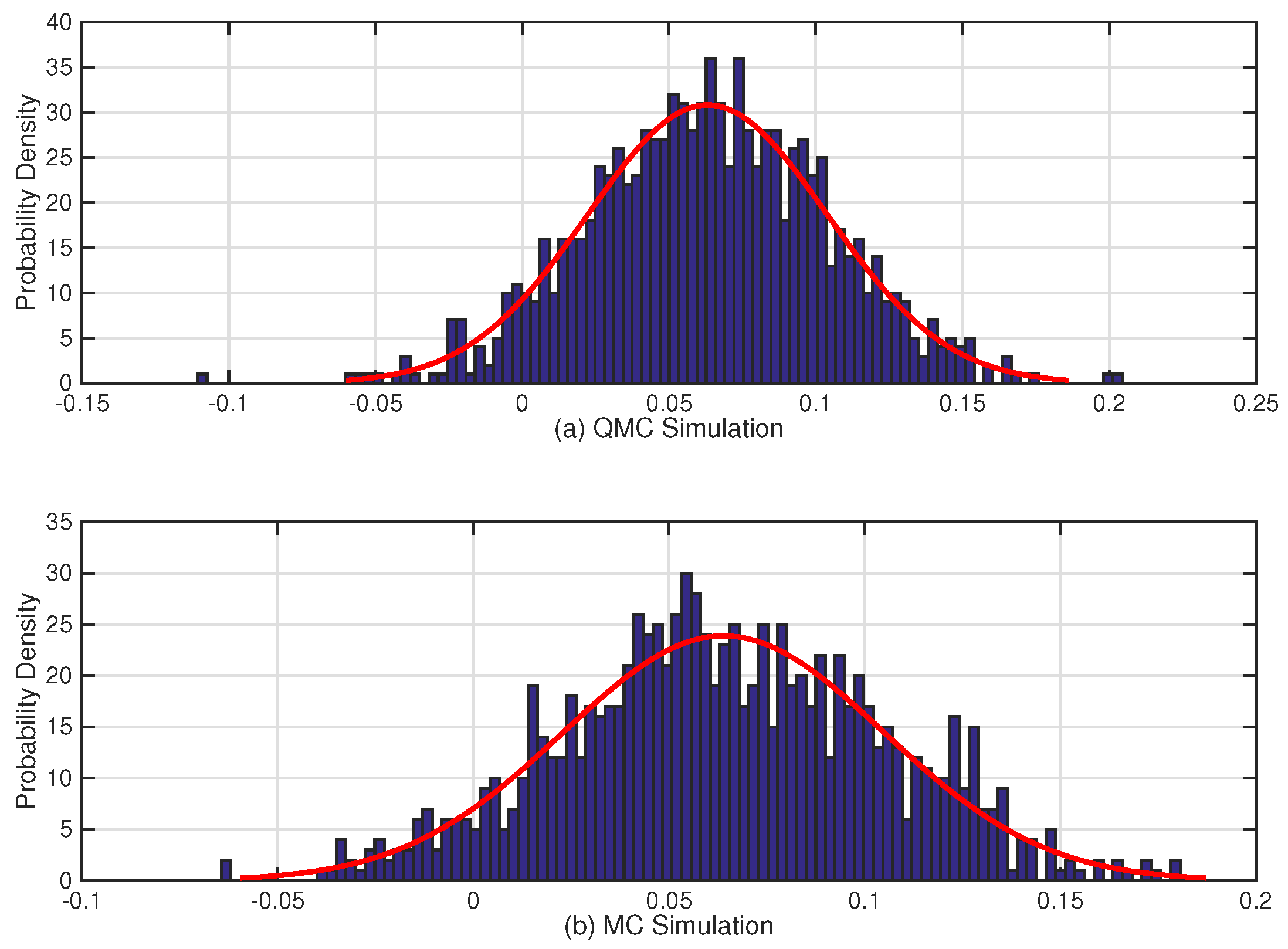
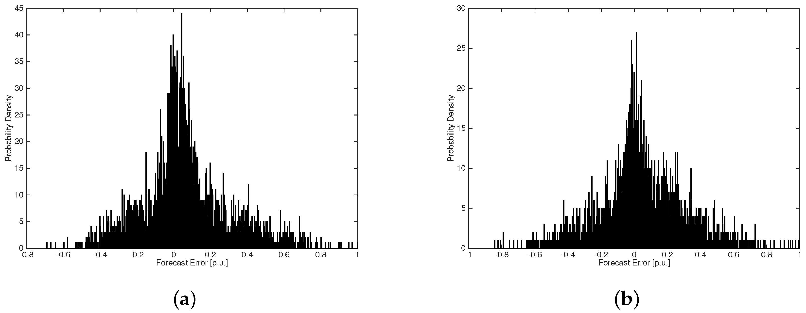
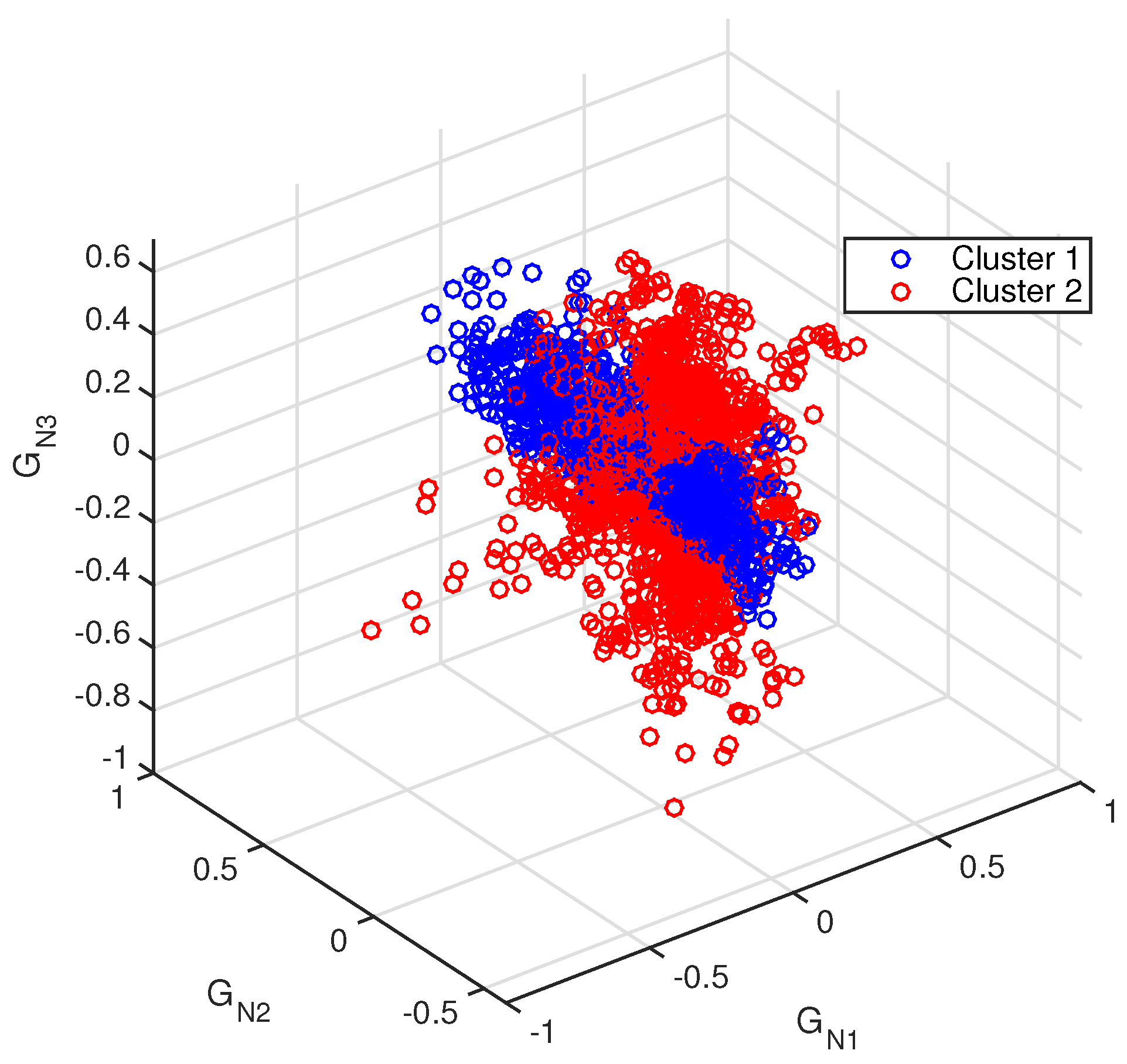
5.1. Statistical Distribution of Wind Power Forecast Error Analysis

The data analyzed in this section are obtained from the amended Renewable Energy Sources (RES) Act (EEG) in Germany [50]. The dataset contains a two-year time series of 15-min projection and the actual value of wind power for 10 wind generations in a wind farm, with around one million data available for analysis, which correspond to the years 2014 and 2015.
Figure 4a,b shows the PDF of forecast error corresponding to the prediction horizon of 1 and 5 h. In the short-term forecast horizon, a particular normal distribution is no longer fitted for the actual forecast error, which is usually used in the probabilistic analysis. Specifically, the shorter the forecast horizon is, the higher the kurtosis is than the others.
The EM algorithm is employed to the Gaussian mixture model, which generates the maximum likelihood estimation of parameters in a statistical model. The clusters of the Gaussian mixture wind power forecast error model for wind generations G N 1 and G N 2 located geomagnetically different for a 1-h and 5-h forecast horizon are presented in Figure 5a,b.
Furthermore, the PDF of the 1 h-ahead forecast error Gaussian mixture distribution for G N 1 is shown in Figure 6. The cluster for 1 h-ahead forecast gathers more closely than the clusters for the 5 h-ahead forecast, which shows that the confidence level of 1 h-ahead forecast error is smaller than that of the 5 h-ahead forecast error. The parameters for the function of the 1 h-ahead forecast error Gaussian mixture distribution for 10 wind generators are shown in Table 1. G N 1 has the largest variance in the average level, which means it has the biggest volatility compared to the other wind generations. Figure 7 describes the 3D clusters of the Gaussian mixture model of wind power forecast error for G N 1 , G N 2 and G N 3 for a 1-h forecast horizon. It shows that in the view of G N 1 , the point sets are distributed more discretely than in other directions.

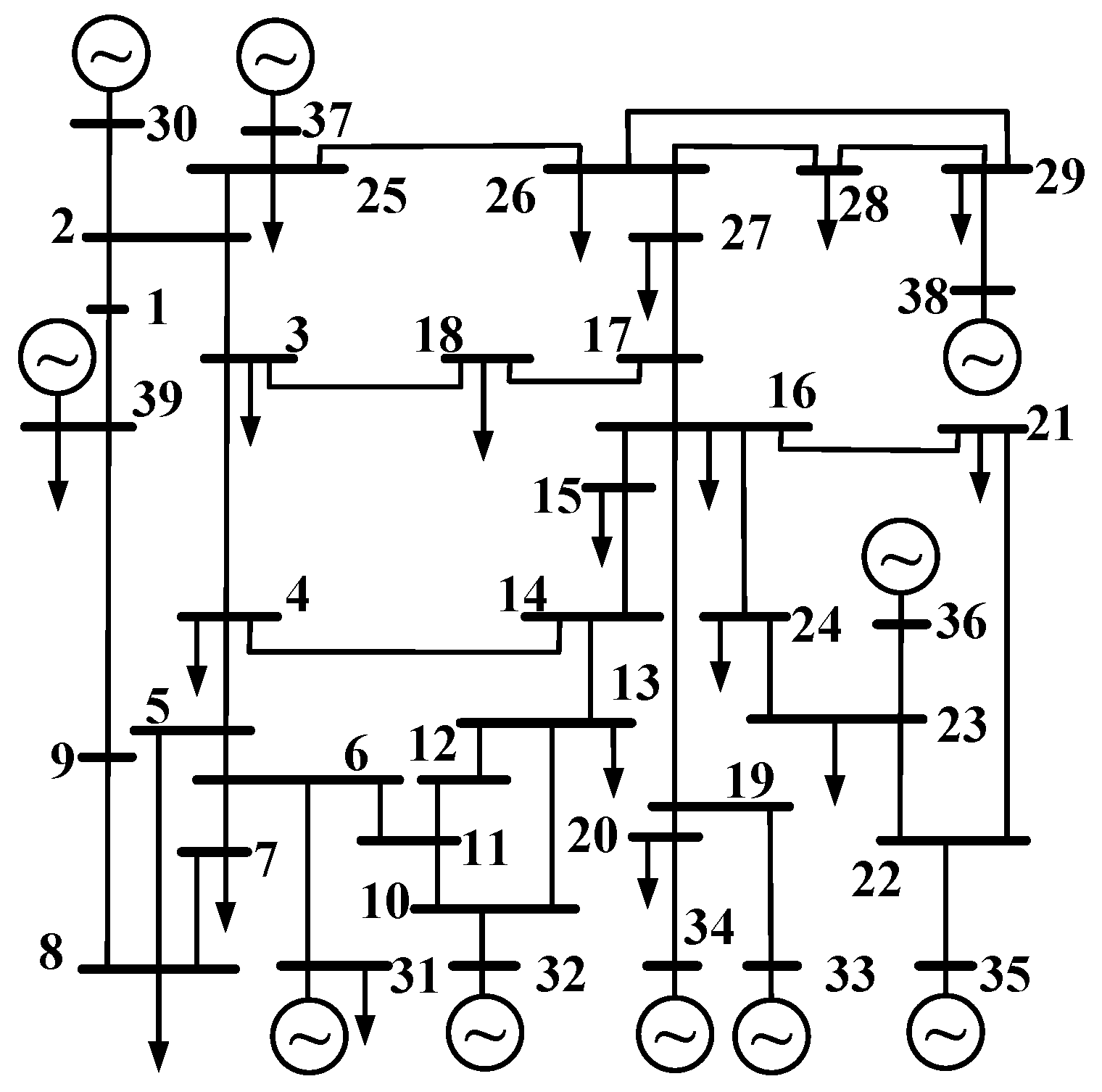
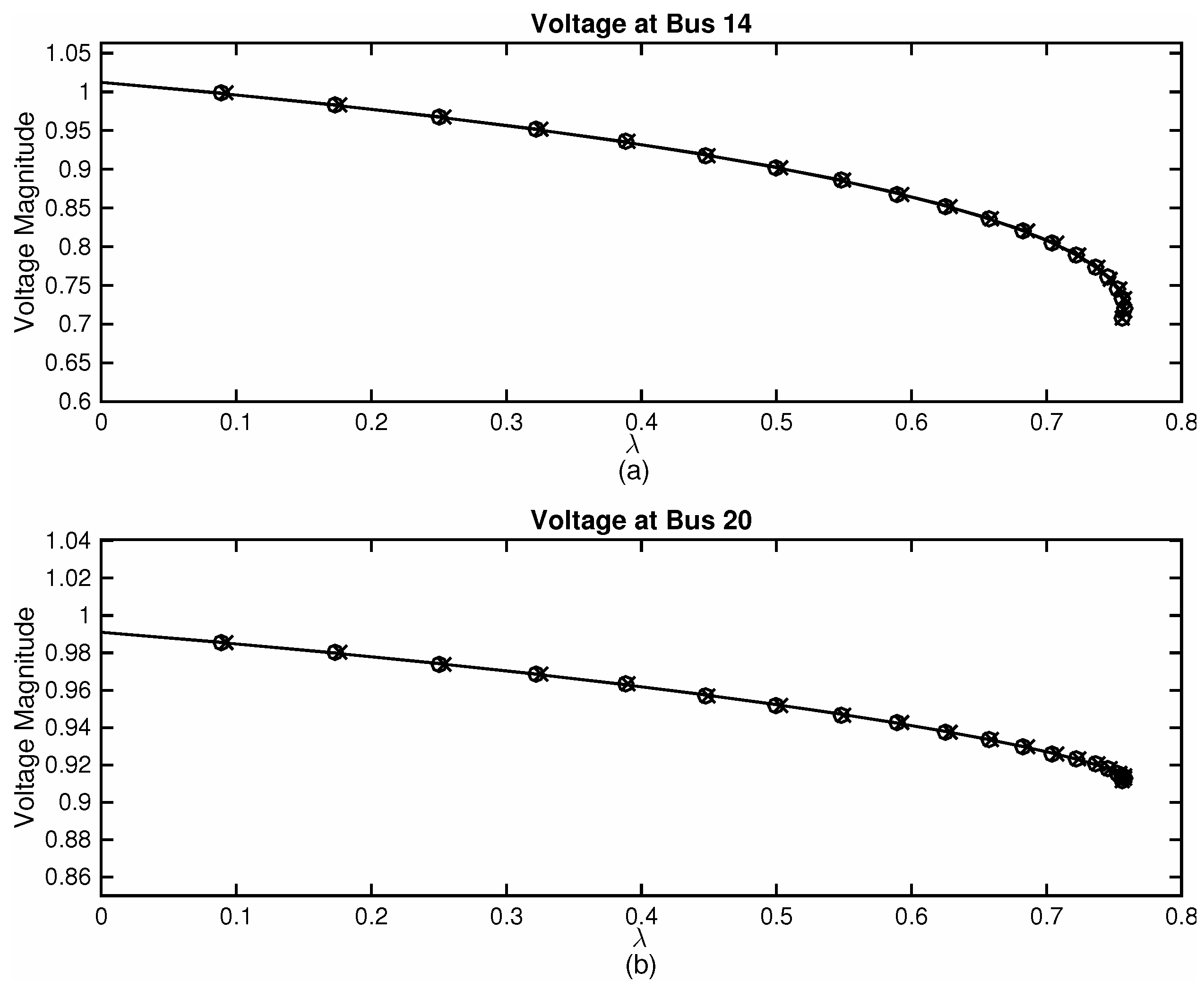
5.2. Case Study: IEEE 39-Bus System

The performance of the proposed algorithm is tested on the IEEE 39 bus New England system [51] in this section. This system consists of 39 buses, 46 lines, 10 units terminal and 29 loads. The wind farms are located at Buses 14, 15 and 30. The rated capacity of each wind farm is 500 WM. Wind generations are fitted for the Gaussian mixture distribution, from which the parameters are obtained in Section 5.1. The network topology of the modified IEEE 39 bus system is given in Figure 8.
Figure 9 shows the comparison between the MC and QMC 1000 times simulation for the probabilistic forecast error model for wind generation G N 1 located at Bus 14. We can figure out that the result of QMC in Figure 9a has less barbs to fit for the Gaussian mixture distribution, which shows that it is closer to the estimated model and has a better performance approach to the actual distribution. However, the results of MC in Figure 9b are worse, which need to sacrifice the efficiency of the computational cost to gain a better performance.
The shape of the magnitude voltage distribution is highly different at different locational buses (in Figure 10), from the perspective of the width of the voltage distribution. The width of the voltage distribution at Bus 15 is three-times larger than the width of the voltage distribution at Bus 30. The peak value of the magnitude at Bus 30 is the most centralized one overall on the whole map of the voltage distribution in the 39-bus system. This is because the randomness comes from the renewable generation at Buses 14, 15 and 30; the voltage at these buses has a longer tail to simulate the worst cases of the small probability events. Besides, the peak value of the magnitudes at Buses 14, 15, 19, 30 is about 0.98675, 0.96188, 1.01094, 1.01143 V, respectively. Besides, the peak value of the phase at Bus 14 is about −52.13 radians. Most of the probability is clustered with respect to this range of phase value. However, the peak value of the phase at Buses 15, 19 and 30 is about −45.59, −42.45, −41.01 radians, respectively.
In addition to this, the shape of the tail is also different for different buses. Even if there is no magnitude or phase out-of-limit event, the risk for each locational voltage is extremely different. The nose curve of the voltage magnitudes at Buses 14 and 20 is compared in Figure 11. The voltage collapse points are 0.710 and 0.915 V, respectively. Then, the index of VaR, CVaR and V RBVSM can be calculated to evaluate the safety-distance from the predicted operational point to the collapse point. The comparison results are shown in Table 2, the sequence of buses is in an ascending order according to the index of V RBVSM to evaluate the weakest voltage bus. The smaller the value of V RBVSM is, the larger the risk of voltage loss is. Hence, Bus 36 is the weakest bus, which may face the voltage out-of-limit event immediately. Additionally, Bus 8 is the strongest bus, which is the safest bus in the IEEE 39-bus system. We should pay more attention to the weakest buses in the system. Several precautions, such as wind curtailment, should be adopted ahead of time.

5.3. Case Study: IEEE 118-Bus System

A modified IEEE 118-bus system is used to study the proposed method. The IEEE 118-bus system has 54 thermal generators, 186 branches and 91 load buses. We assume that three wind turbines are located at Buses 15, 54 and 96. The system topology is given in [52].
The computational cost of the proposed algorithm is approximately 40.17 s via 200 times QMC simulation. However, the computational cost of the method complemented with the same convergence rate via MC runs is about 8000.52 s, which runs the MC simulation 40,000 times. The convergence rate compared between QMC and MC is shown in Figure 12a.
We make a comparison of our proposed method (Method 1) and a conventional risk-based approach (Method 2) [53]. The work in [53] gives a process of voltage instability risk calculation for a given contingency:
(1)
Run continuation power flow to obtain the expected value of the loadability;
(2)
Compute loadability sensitivities;
(3)
Get the PDF for Pr (%margin) = Pr [ Loadability Forecast / Forecast ] ;
(4)
Obtain the risk index Risk = Pr ( % margin ) × Sev ( % margin ) ;
(5)
Store the risk index.
The indices of VaR, CVaR and V RBVSM of the voltage magnitudes are shown in Table 3 to evaluate the weakest 20 buses in the IEEE 118-bus system. The risk of voltage out-of-limit events at these buses is larger than the risk of voltage loss at any other buses. However, using Method 2, they only give one risk index value for measuring voltage instability in a particular case. The weakest bus is Bus 24, the same as the result using Method 1. Furthermore, the risk index of Bus 24 is equal to 11. Besides, the risk index for other buses is equal to zero. The index proposed in Method 2 is not as sensitive as the index using Method 1. As shown in Table 3, the ranking of the 20 weakest buses is listed to support the system operators to pay attention to these buses. Even though Method 2 can identify the weakest bus and using the risk index for measuring the weakest bus as the final result, it is hard for Method 2 to identify the weakest area or to help the system operators to perform preventive control as if the voltage instability may happen in a different area.
We assume that the nodal load of the IEEE 118-bus system is fitted for the California ‘duck curve’-nodal load curve as shown in Figure 12b. In order to evaluate the magnitudes at the weakest Bus 24, we obtain the index of V RBVSM as shown in Figure 13 according to the time varying wind power output forecast for each 5 min. As we know, when the value of V RBVSM is closer to zero, the probability of a voltage collapse event happening at that particular point is higher. In this scenario, the nodal load reaches the peak value at the last 1 h, as the value of V RBVSM decreases to the lowest level in the same time period.

6. Summary and Conclusions

In the operation of today’s electricity power system, the on-line security of the operation is still the most significant issue, especially in an uncertain environment. This paper develops a risk-based statistic voltage evaluation mechanism. Different from the conventional deterministic evaluation method, the powerful risk-based voltage statistic index V RBVSM provides the relative safety distance to the voltage collapse point on the system risk level considering the tail risk of the voltage stability loss. Using this voltage evaluation index results in more secure operating conditions when the precaution has been made ahead of serious events happening. The new voltage evaluation approach was illustrated and compared in both the IEEE 39-bus system and the IEEE 118-bus system. In both cases, the proposed method provides a more conservative result depending on the forecast estimation for the near future. While the parameter of the wind power output forecast error distribution has been studied, the real-time probabilistic voltage forecast can be simulated based on the QMC sampling techniques to speed up the whole approach. Furthermore, the voltage index proposed in this paper offers an alternative approach based on the real-time probabilistic voltage forecast method. The approach avoids the effect of small probability serious events on voltage spikes while providing control to enhance the system security level. The proposed method is of great value in the application of real-time economic dispatch, system security prevention and control in the future.

Acknowledgments

This research is supported by the National High Technology Research and Development of China (863 Program) (No. 2015AA050201). The authors also thank Beth Larson for her constructive comments and suggestions.

Author Contributions

Weisi Deng and Buhan Zhang conceived and designed the experiments; Weisi Deng performed the experiments; Buhan Zhang and Hongfa Ding contributed materials and analysis tools; Weisi Deng wrote the paper; Hang Li analyzed the data and revised the paper.

Conflicts of Interest

The authors declare no conflict of interest.

References

  1. Abe, S.; Fukunaga, Y.; Isono, A.; Kondo, B. Power system voltage stability. IEEE Trans. Power Appar. Syst. 1982, PAS-101, 3830–3840. [Google Scholar] [CrossRef]
  2. Almeida, A.B.; De Lorenci, E.V.; Leme, R.C.; De Souza, A.C.Z.; Lopes, B.I.L.; Lo, K. Probabilistic voltage stability assessment considering renewable sources with the help of the PV and QV curves. IET Renew. Power Gener. 2013, 7, 521–530. [Google Scholar] [CrossRef]
  3. Wan, H.; McCalley, J.D.; Vittal, V. Risk based voltage security assessment. IEEE Trans. Power Syst. 2000, 15, 1247–1254. [Google Scholar] [CrossRef]
  4. Beiraghi, M.; Ranjbar, A. Online voltage security assessment based on wide-area measurements. IEEE Trans. Power Deliv. 2013, 28, 989–997. [Google Scholar] [CrossRef]
  5. Dissanayaka, A.; Annakkage, U.D.; Jayasekara, B.; Bagen, B. Risk-based dynamic security assessment. IEEE Trans. Power Syst. 2011, 26, 1302–1308. [Google Scholar] [CrossRef]
  6. Kirschen, D.; Jayaweera, D. Comparison of risk-based and deterministic security assessments. IET Gener. Transm. Distrib. 2007, 1, 527–533. [Google Scholar] [CrossRef]
  7. Li, W. Risk assessment of power systems: Models, methods, and applications; John Wiley & Sons: Hoboken, NJ, USA, 2014. [Google Scholar]
  8. Ciapessoni, E.; Cirio, D.; Kjølle, G.; Massucco, S.; Pitto, A.; Sforna, M. Probabilistic risk-based security assessment of power systems considering incumbent threats and uncertainties. IEEE Trans. Smart Grid 2016, 7, 2890–2903. [Google Scholar] [CrossRef]
  9. Li, X.; Zhang, X.; Wu, L.; Lu, P.; Zhang, S. Transmission line overload risk assessment for power systems with wind and load-power generation correlation. IEEE Trans. Smart Grid 2015, 6, 1233–1242. [Google Scholar] [CrossRef]
  10. Preece, R.; Milanović, J.V. Probabilistic risk assessment of rotor angle instability using fuzzy inference systems. IEEE Trans. Power Syst. 2015, 30, 1747–1757. [Google Scholar] [CrossRef]
  11. Aldeen, M.; Saha, S.; Alpcan, T.; Evans, R. New online voltage stability margins and risk assessment for multi-bus smart power grids. Int. J. Control 2015, 88, 1338–1352. [Google Scholar] [CrossRef]
  12. Alpcan, T.; Saha, S.; Aldeen, M. Assessment of voltage stability risks under intermittent renewable generation. In Proceedings of the 2014 IEEE PES General Meeting|Conference & Exposition, Metro Area, Washington, DC, USA, 27–31 July 2014; pp. 1–5.
  13. Aldeen, M.; Saha, S.; Alpcan, T. Voltage stability margins and risk assessment in smart power grids. IFAC Proc. Vol. 2014, 47, 8188–8195. [Google Scholar] [CrossRef]
  14. Rodrigues, A.B.; Prada, R.B.; da Guia da Silva, M. Voltage stability probabilistic assessment in composite systems: Modeling unsolvability and controllability loss. IEEE Trans. Power Syst. 2010, 25, 1575–1588. [Google Scholar] [CrossRef]
  15. Chen, P.C.; Malbasa, V.; Kezunovic, M. Analysis of voltage stability issues with distributed generation penetration in distribution networks. In Proceedings of the 45th North American Power Symp, Manhattan, NY, USA, 22–24 September 2013; pp. 1–7.
  16. Yu, J.; Li, W.; Yan, W.; Zhao, X.; Ren, Z. Evaluating risk indices of weak lines and buses causing static voltage instability. In Proceedings of the 2011 IEEE Power and Energy Society General Meeting, Detroit, MI, USA, 24–28 July 2011; pp. 1–7.
  17. Bienstock, D.; Chertkov, M.; Harnett, S. Chance-constrained optimal power flow: Risk-aware network control under uncertainty. SIAM Rev. 2014, 56, 461–495. [Google Scholar] [CrossRef]
  18. Zhang, Y.; Giannakis, G.B. Distributed stochastic market clearing with high-penetration wind power. IEEE Trans. Power Syst. 2016, 31, 895–906. [Google Scholar] [CrossRef]
  19. Allan, R.; Al-Shakarchi, M.G. Probabilistic techniques in ac load-flow analysis. Electr. Eng. Proc. Inst. 1977, 124, 154–160. [Google Scholar] [CrossRef]
  20. Zhang, P.; Lee, S.T. Probabilistic load flow computation using the method of combined cumulants and Gram-Charlier expansion. IEEE Trans. Power Syst. 2004, 19, 676–682. [Google Scholar] [CrossRef]
  21. Hu, Z.; Wang, X. A probabilistic load flow method considering branch outages. IEEE Trans. Power Syst. 2006, 21, 507–514. [Google Scholar] [CrossRef]
  22. Gao, L.; Wu, J. Voltage risk evaluation based on improved probabilistic load flow considering intermittent wind farm. In Proceedings of the 2012 Asia-Pacific Power and Energy Engineering Conference, Shanghai, China, 27–29 March 2012; pp. 1–4.
  23. Morales, J.M.; Perez-Ruiz, J. Point estimate schemes to solve the probabilistic power flow. IEEE Trans. Power Syst. 2007, 22, 1594–1601. [Google Scholar] [CrossRef]
  24. Singhee, A.; Rutenbar, R.A. Why quasi-monte carlo is better than monte carlo or latin hypercube sampling for statistical circuit analysis. IEEE Trans. Comput.-Aided Des. Integr. Circuits Syst. 2010, 29, 1763–1776. [Google Scholar] [CrossRef]
  25. Wu, J.; Zhang, B.; Deng, W.; Zhang, K. Application of cost-cvar model in determining optimal spinning reserve for wind power penetrated system. Int. J. Electr. Power Energy Syst. 2015, 66, 110–115. [Google Scholar] [CrossRef]
  26. Deng, W.; Ding, H.; Zhang, B.; Lin, X.; Bie, P.; Wu, J. Multi-period probabilistic-scenario risk assessment of power system in wind power uncertain environment. IET Gener. Transm. Distrib. 2016, 10, 359–365. [Google Scholar] [CrossRef]
  27. Wang, Z.; Bian, Q.; Xin, H.; Gan, D. A Distributionally Robust Co-Ordinated Reserve Scheduling Model Considering CVaR-Based Wind Power Reserve Requirements. IEEE Trans. Sustain. Energy 2016, 7, 625–636. [Google Scholar] [CrossRef]
  28. Rockafellar, R.T.; Uryasev, S. Optimization of conditional value-at-risk. J. Risk 2000, 2, 21–42. [Google Scholar] [CrossRef]
  29. Uryasev, S. Conditional value-at-risk: Optimization algorithms and applications. In Proceedings of the IEEE/IAFE/INFORMS 2000 Conference on Computational Intelligence for Financial Engineering, New York, NY, USA, 26–28 March 2000; pp. 49–57.
  30. Sirisena, H.; Brown, E. Representation of non-Gaussian probability distributions in stochastic load-flow studies by the method of Gaussian sum approximations. IEE Proc. C-Gener. Transm. Distrib. 1983, 130, 165–171. [Google Scholar] [CrossRef]
  31. Ke, D.; Chung, C.; Sun, Y. A novel probabilistic optimal power flow model with uncertain wind power generation described by customized Gaussian mixture model. IEEE Trans. Sustain. Energy 2016, 7, 200–212. [Google Scholar] [CrossRef]
  32. Valverde, G.; Saric, A.; Terzija, V. Probabilistic load flow with non-Gaussian correlated random variables using Gaussian mixture models. IET Gener. Transm. Distrib. 2012, 6, 701–709. [Google Scholar] [CrossRef]
  33. Singh, R.; Pal, B.C.; Jabr, R.A. Statistical representation of distribution system loads using Gaussian mixture model. IEEE Trans. Power Syst. 2010, 25, 29–37. [Google Scholar] [CrossRef]
  34. Bilmes, J.A. A Gentle Tutorial of the EM Algorithm and Its Application to Parameter Estimation for Gaussian Mixture and Hidden Markov Models; International Computer Science Institute: Berkeley, CA, USA, 1998. [Google Scholar]
  35. Celeux, G.; Diebolt, J. A stochastic approximation type EM algorithm for the mixture problem. Stochastics 1992, 41, 119–134. [Google Scholar] [CrossRef]
  36. Elia. Available online: http://www.elia.be/ (accessed on 23 January 2017).
  37. Dobson, I.; Van Cutsem, T.; Vournas, C.; DeMarco, C.; Venkatasubramanian, M.; Overbye, T.; Canizares, C. Voltage stability assessment: Concepts, practices and tools. IEEE Power Eng. Soc. Power Syst. Stab. Subcomm. Spec. Publ. 2002, 11, 21–22. [Google Scholar]
  38. Beck, M.; Kewell, B. Risk: A Study of Its Origins, History and Politics; World Scientific: Hackensack, NJ, USA, 2014. [Google Scholar]
  39. Palmquist, J.; Uryasev, S.; Krokhmal, P. Portfolio Optimization With Conditional Value-at-Risk Objective and Constraints; Department of Industrial & Systems Engineering, University of Florida: Gainesville, FL, USA, 1999. [Google Scholar]
  40. Van der Veen, R.A.; Abbasy, A.; Hakvoort, R.A. Agent-based analysis of the impact of the imbalance pricing mechanism on market behavior in electricity balancing markets. Energy Econ. 2012, 34, 874–881. [Google Scholar] [CrossRef]
  41. Dabbagh, S.R.; Sheikh-El-Eslami, M.K. Risk Assessment of Virtual Power Plants Offering in Energy and Reserve Markets. IEEE Trans. Power Syst. 2016, 31, 3572–3582. [Google Scholar] [CrossRef]
  42. Xue, Y.; Manjrekar, M.; Lin, C.; Tamayo, M.; Jiang, J.N. Voltage stability and sensitivity analysis of grid-connected photovoltaic systems. In Proceedings of the 2011 IEEE Power and Energy Society General Meeting, Detroit, MI, USA, 24–28 July 2011; pp. 1–7.
  43. Glasserman, P. Monte Carlo Methods in Financial Engineering; Springer: Heidelberg, Germany, 2003; Volume 53. [Google Scholar]
  44. Niederreiter, H. Quasi-Monte Carlo methods and pseudo-random numbers. Bull. Am. Math. Soc. 1978, 84, 957–1041. [Google Scholar] [CrossRef]
  45. Morokoff, W.J.; Caflisch, R.E. Quasi-random sequences and their discrepancies. SIAM J. Sci. Comput. 1994, 15, 1251–1279. [Google Scholar] [CrossRef]
  46. Owen, A.B. Quasi-monte carlo sampling. Monte Carlo Ray Tracing Siggraph 2003, 1, 69–88. [Google Scholar]
  47. Caflisch, R.E. Monte carlo and quasi-monte carlo methods. Acta Numer. 1998, 7, 1–49. [Google Scholar] [CrossRef]
  48. Chung, K.L. An estimate concerning the kolmogroff limit distribution. Trans. Am. Math. Soc. 1949, 67, 36–50. [Google Scholar] [CrossRef]
  49. Huang, H.; Chung, C.; Chan, K.W.; Chen, H. Quasi-Monte Carlo based probabilistic small signal stability analysis for power systems with plug-in electric vehicle and wind power integration. IEEE Trans. Power Syst. 2013, 28, 3335–3343. [Google Scholar] [CrossRef]
  50. Date of Wind Projection and Actual Value by TransnetBW. Available online: https://www.transnetbw.com/en/key-figures/renewable-energies/wind-infeed (accessed on 23 January 2017).
  51. Pai, A. Energy Function Analysis for Power System Stability; Springer: Heidelberg, Germany, 2012. [Google Scholar]
  52. Gonzalez-Longatt, F.M. IEEE 118 Bus Test. Available online: http://fglongatt.org/OLD/TestCaseIEEE118. html (accessed on 19 March 2015).
  53. Ni, M.; McCalley, J.D.; Vittal, V.; Tayyib, T. Online risk-based security assessment. IEEE Trans. Power Syst. 2003, 18, 258–265. [Google Scholar] [CrossRef]
Figure 1. Comparison of the histogram of 15-min forecast error with the Gaussian mixture distribution using historical data on [36].
Energies 10 00180 g001
Figure 2. The relationship between transmitted power and receiving end voltage (PV curve).
Energies 10 00180 g002
Figure 3. The comparison of VaR and CVaR .
Energies 10 00180 g003
Figure 4. (a) A histogram of 1 h-ahead measured wind forecast error; and (b) a histogram of 5 h-ahead measured wind forecast error.
Energies 10 00180 g004
Figure 5. The clusters of the Gaussian mixture wind power forecast error model for (a) 1-h and (b) 5-h horizon (the cluster means the sample sets fit for one particular Gaussian distribution).
Energies 10 00180 g005
Figure 6. The Gaussian mixture wind power forecast error distribution for a 1-h horizon.
Energies 10 00180 g006
Figure 7. The three-dimensional clusters of the Gaussian mixture model of wind power forecast error for a 1-h horizon.
Energies 10 00180 g007
Figure 8. IEEE New England 39-bus system.
Energies 10 00180 g008
Figure 9. The comparison between the (a) QMC and (b) MC simulation of the Gaussian mixture wind forecast error model for wind generation G N 1 at Bus 14 (1000 times).
Energies 10 00180 g009
Figure 10. The voltage magnitudes distribution at different buses in the 39-bus system (voltage magnitudes/p.u. vs. probability density).
Energies 10 00180 g010
Figure 11. The nose curve of voltage magnitudes at Buses 14 and 20.
Energies 10 00180 g011
Figure 12. (a) The convergence rate for QMC and MC sampling (0.005 is the rate of convergence); and (b) the duck curve of nodal load in the California power system.
Energies 10 00180 g012
Figure 13. The index of V RBVSM at Bus 24 according to the duck curve nodal load at risk level β = 95 % .
Energies 10 00180 g013
Table 1. The parameters of the 1 h-ahead forecast error Gaussian mixture distribution for 10 wind generations.
Generation μ 1 σ 1 ϖ 1 μ 2 σ 2 ϖ 2
G N 1 0.03740.05150.45570.08530.06090.5443
G N 2 −0.10420.03340.4557−0.05340.01180.5443
G N 3 0.03310.03150.45570.00720.02250.5443
G N 4 −0.06790.04910.45570.02150.00450.5443
G N 5 0.00960.02090.45570.02150.00580.5443
G N 6 0.00960.02090.45570.02570.00580.5443
G N 7 −0.03220.02670.45570.02570.06930.5443
G N 8 0.07410.07830.45570.10680.01400.5443
G N 9 −0.04270.02280.45570.05180.04200.5443
G N 10 −0.01910.00660.4557−0.02110.02030.5443
Table 2. The indices of VaR, CVaR and V RBVSM for evaluating the weakest 10 buses at the risk level β = 95 % .
Index of BusesVaRCVaR V RBVSM
361.00801.05630.0047
351.00581.05000.0052
381.00991.04150.0165
311.00041.01120.0298
321.00201.01250.0342
331.00221.01840.0456
341.00411.02200.0509
371.00941.03100.0531
220.97710.97850.0839
230.97830.97170.0958
Table 3. The indices of VaR, CVaR and V RBVSM for evaluating the weakest 20 buses at the risk level β = 95 % .
Index of BusesVaRCVaR V RBVSM
240.960090.975450.00010
80.943810.976040.00013
610.980000.980780.00014
480.970000.989780.00016
250.960360.992560.00028
620.980110.984290.00042
590.980000.982150.00049
260.961150.966600.00055
230.960020.965330.00063
670.984410.985250.00079
600.980000.980790.00080
40.938720.939440.00081
50.942180.945750.00091
90.944360.962810.00091
660.984000.991400.00092
500.971000.976900.00096
460.969300.985130.00096
730.985000.985880.00096
470.969440.982280.00096
490.970000.997350.00097

