
Discrete Fracture Network Modelling in a Naturally Fractured Carbonate Reservoir in the Jingbei Oilfield, China

Abstract
:1. Introduction
2. Data and Methodology
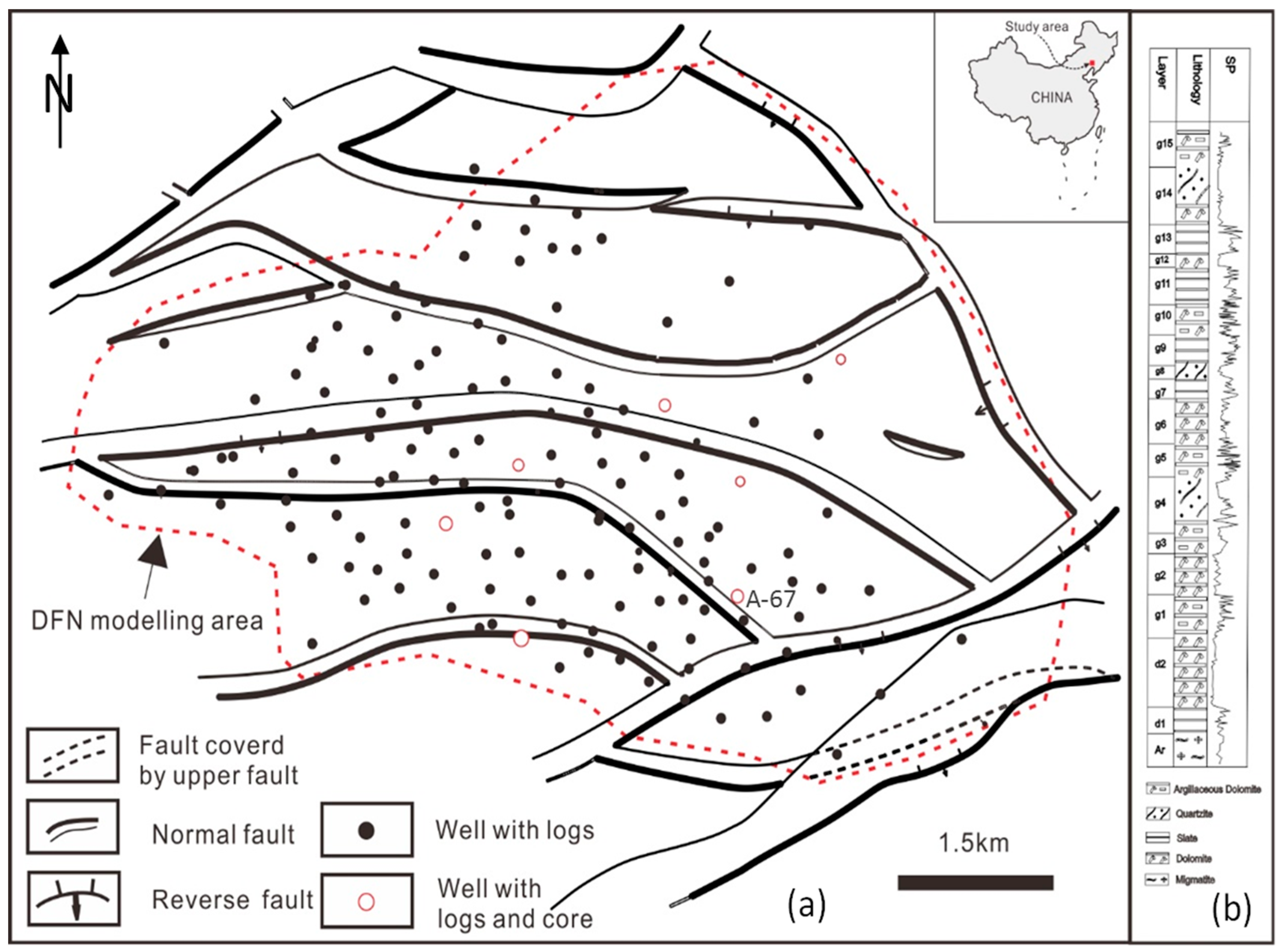
2.1. Geological Settings for Jingbei Oilfield
2.2. Data
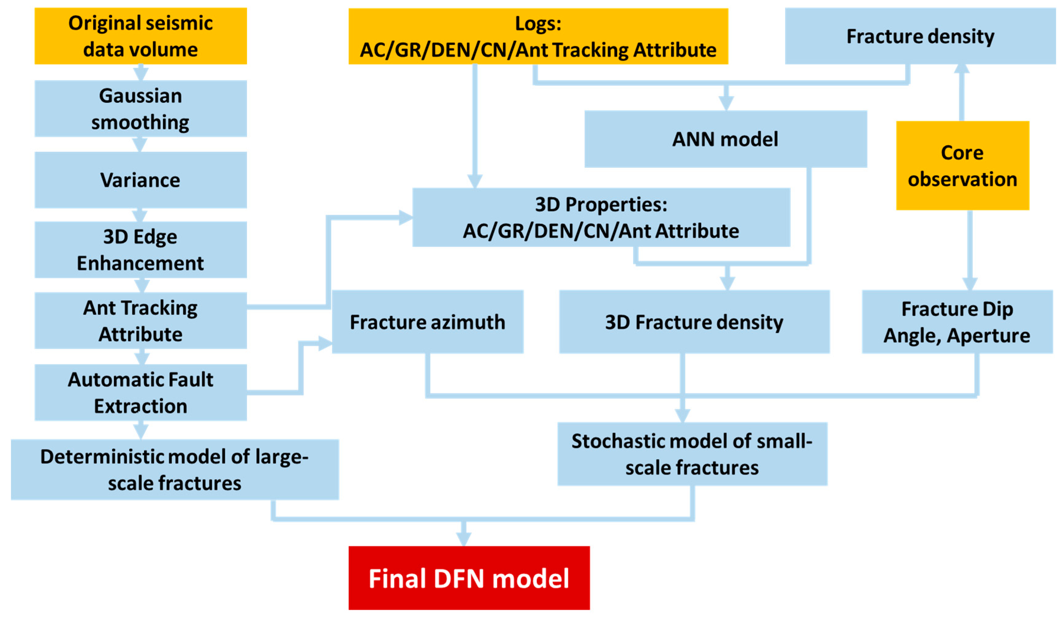
2.3. Methodology
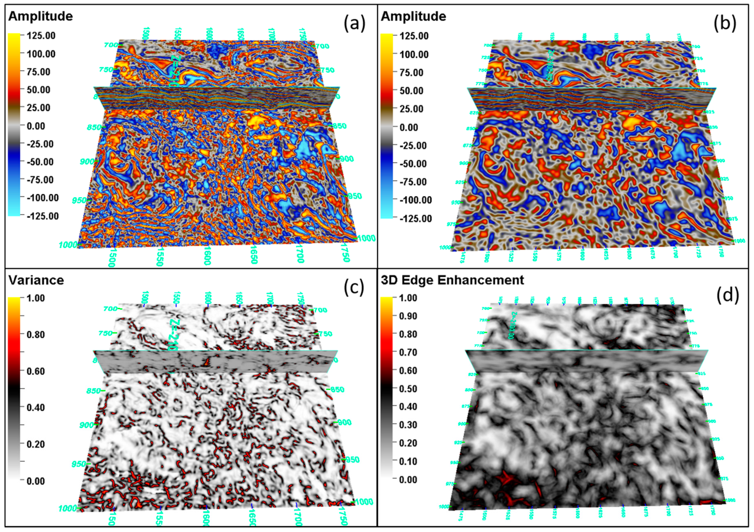
2.3.1. Condition of the Seismic Data Volume
2.3.2. Ant Tracking Algorithm
2.3.3. Extraction of the Faults and Fractures
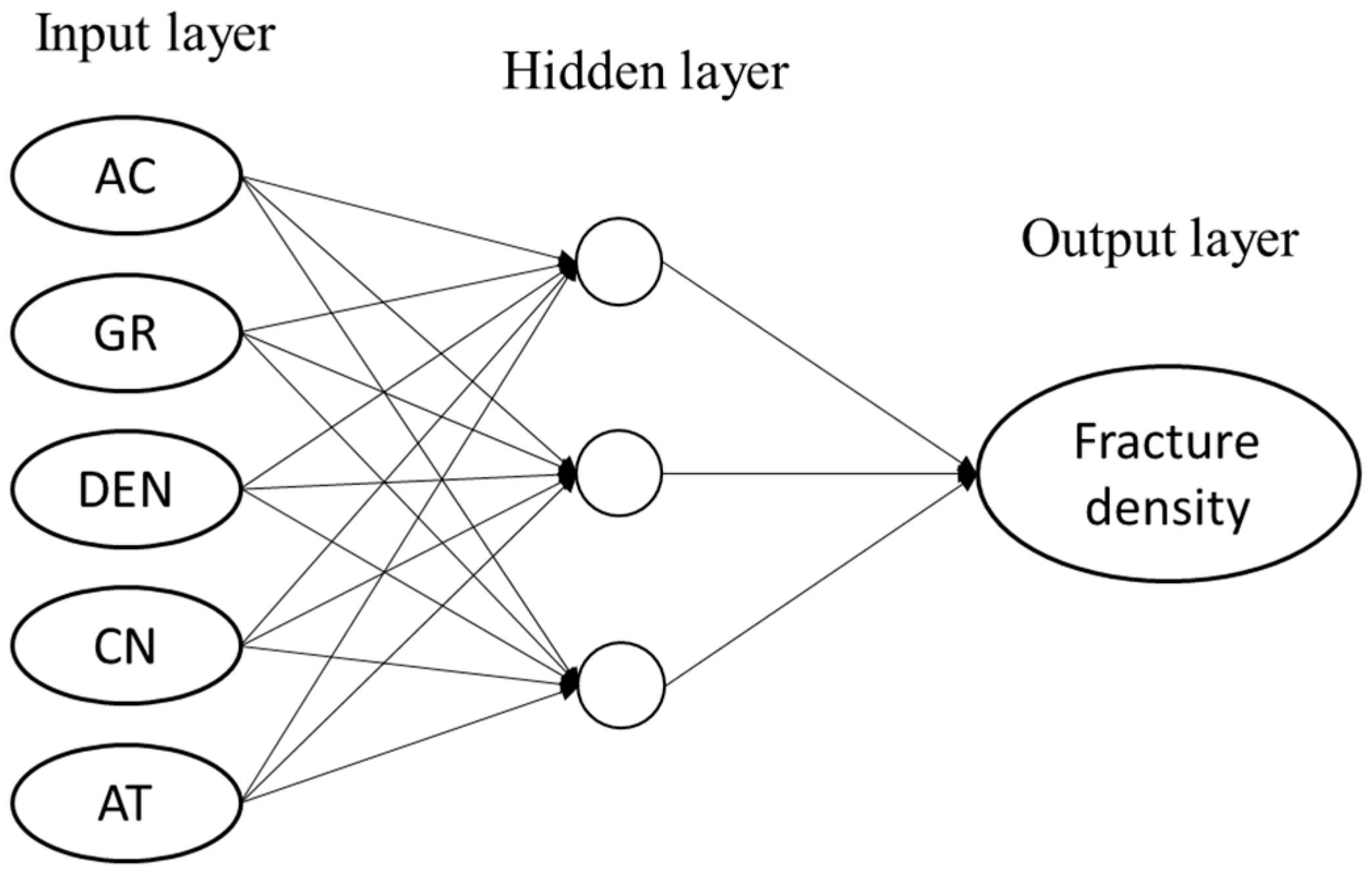
2.3.4. Artificial Neural Network
2.3.5. Discrete Fracture Modelling
2.3.6. Core Observation and Analysis
3. Results and Discussion
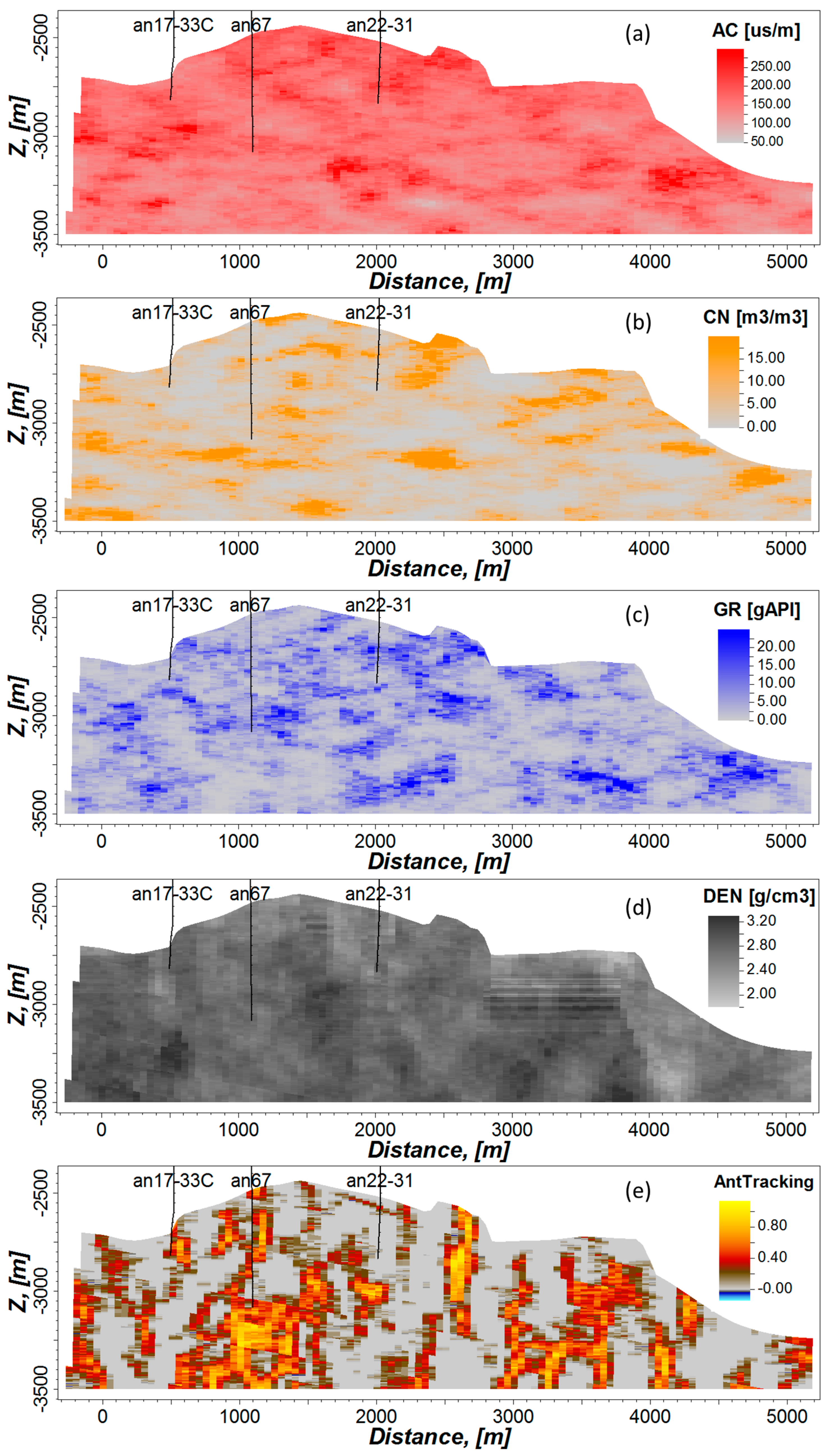
3.1. Seismic Conditions
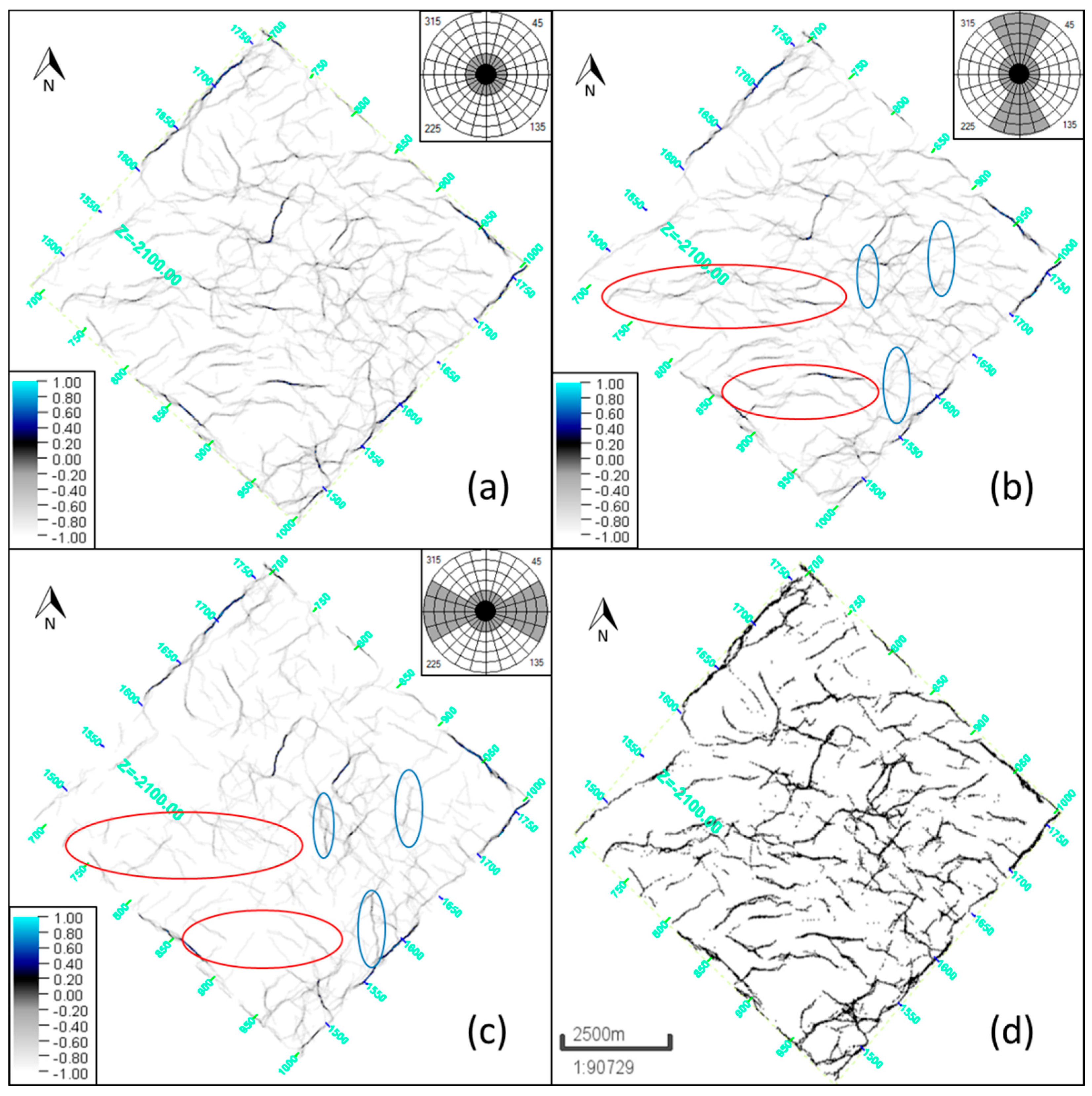
3.2. Ant Tracking Result
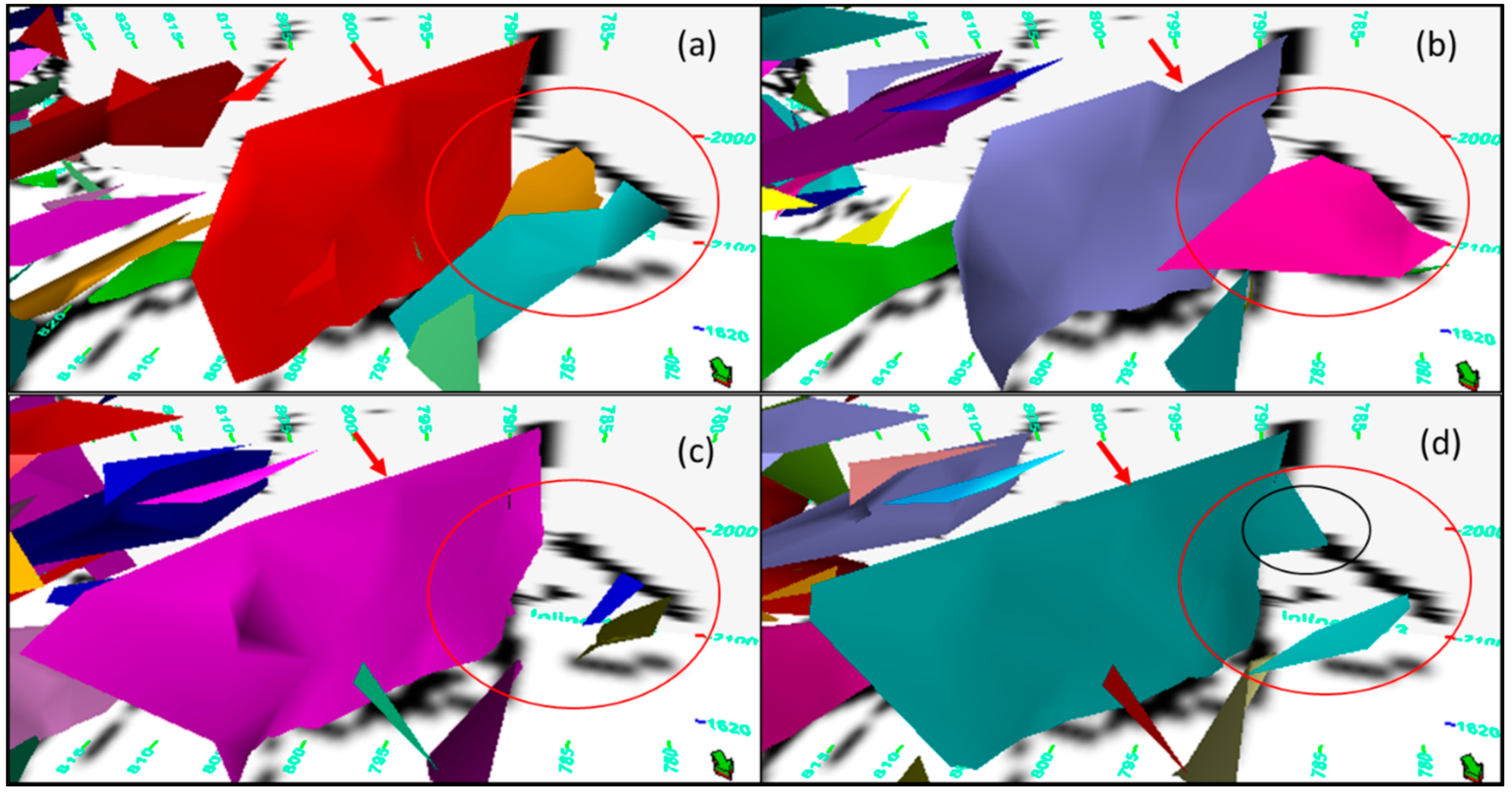
3.3. Extraction of the Large-Scale Fractures
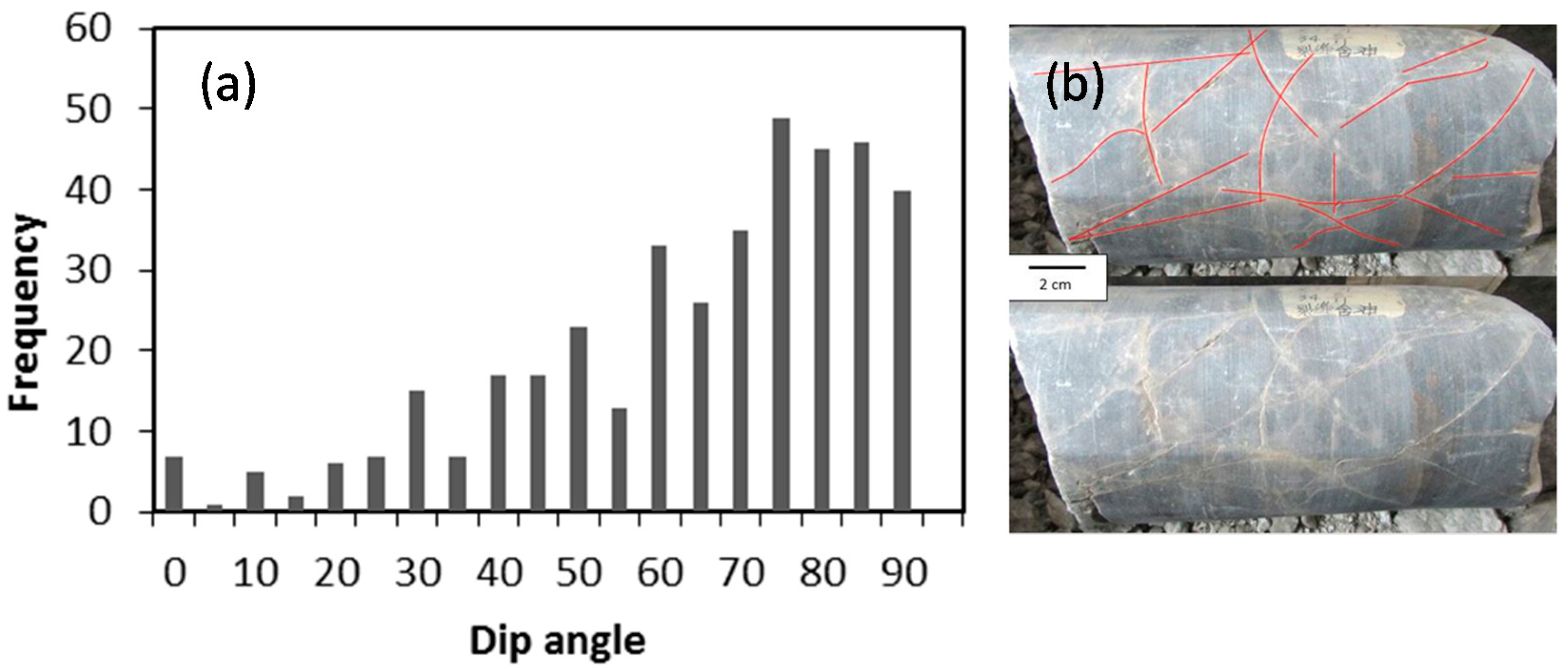
3.4. Core Observation Result
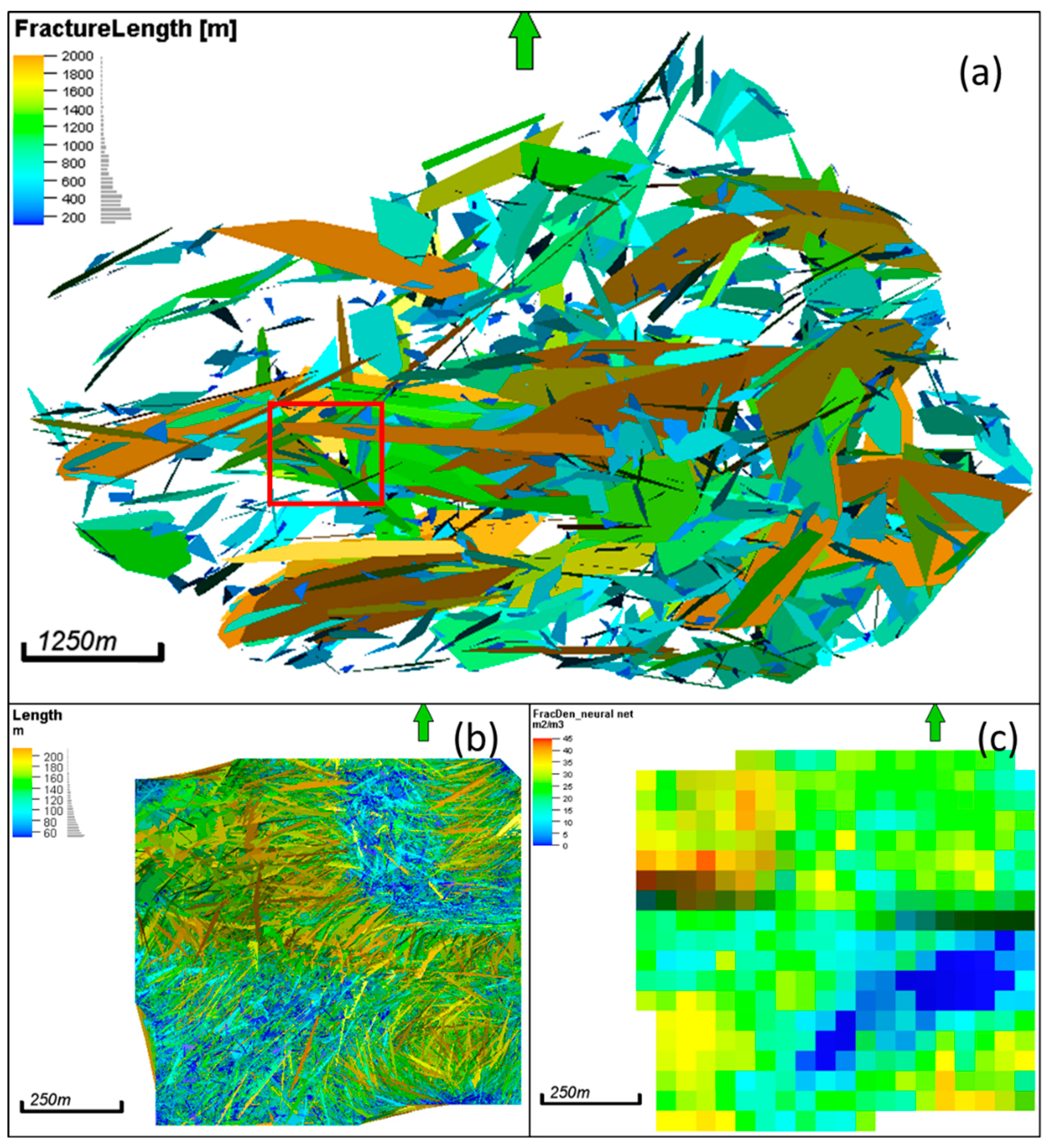
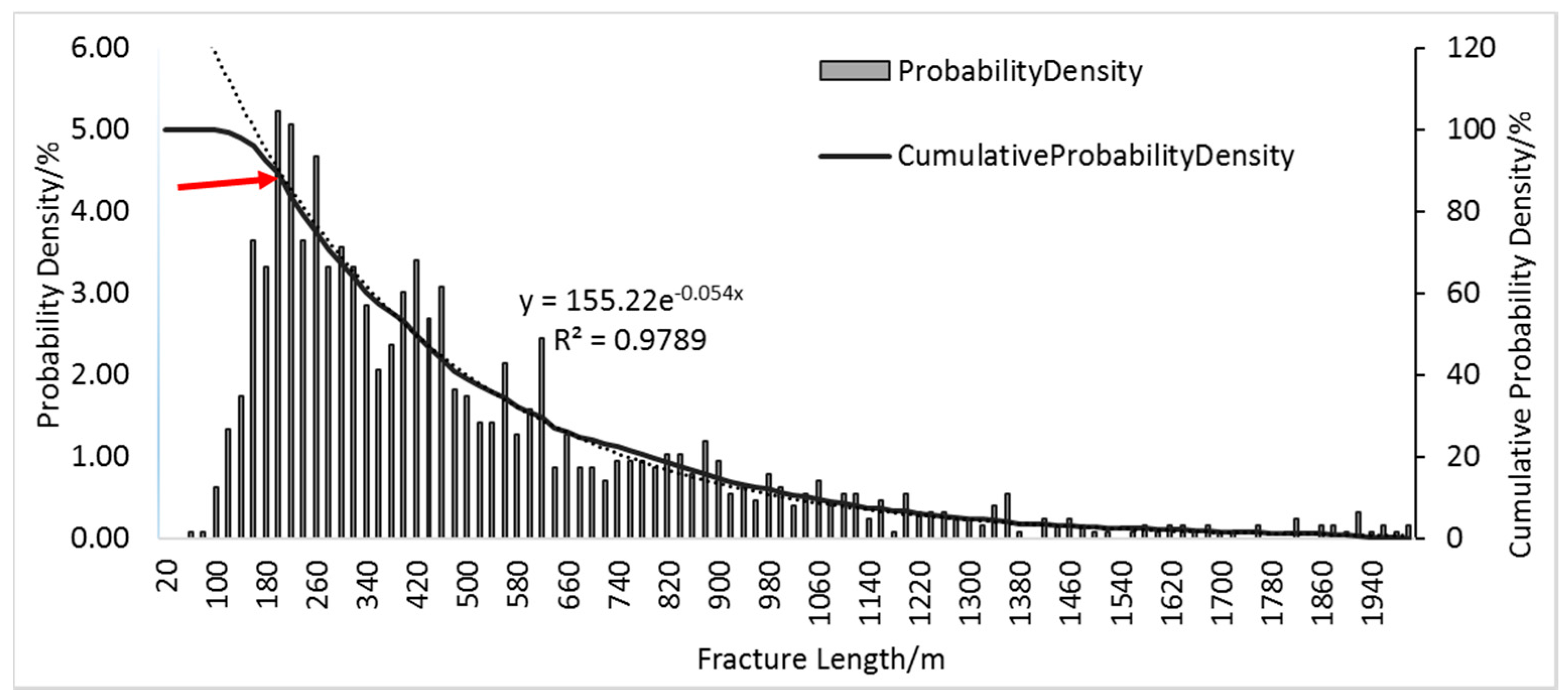
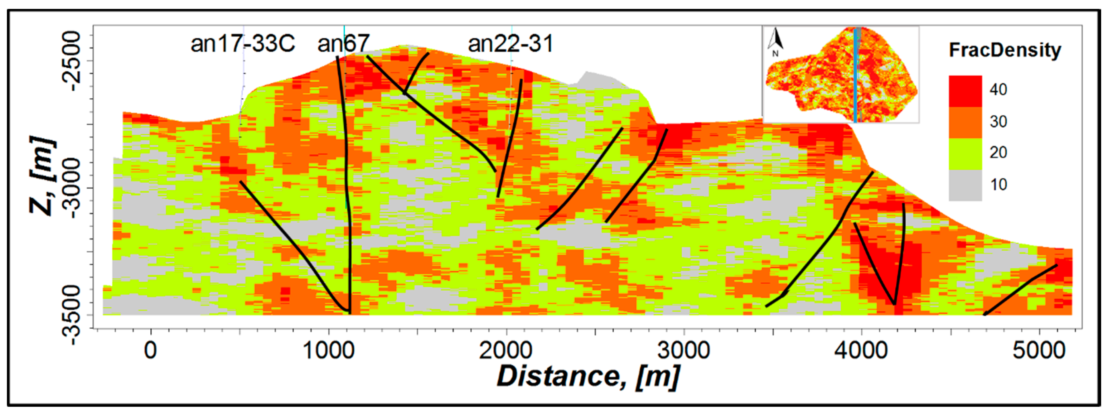
3.5. Fracture Density Distribution
3.6. DFN Modelling
4. Conclusions
- (1)
- The ant tracking attribute is feasible to detect the small faults and large-scale fractures in the buried hill reservoir. Before using the ant tracking algorithm, the seismic condition processes are necessary to enhance the quality of the seismic data;
- (2)
- The variance attribute is a powerful method to detect the edge of the amplitude volume, which is essential to the ant tracking process. Particularly, we tried an automatic workflow to extract the faults and fractures detected by the ants. The automatical workflow can save computing time, although we lost some accuracy since the shape and the position of the fractures do not always follow the discontinuity of the ant tracking attribute;
- (3)
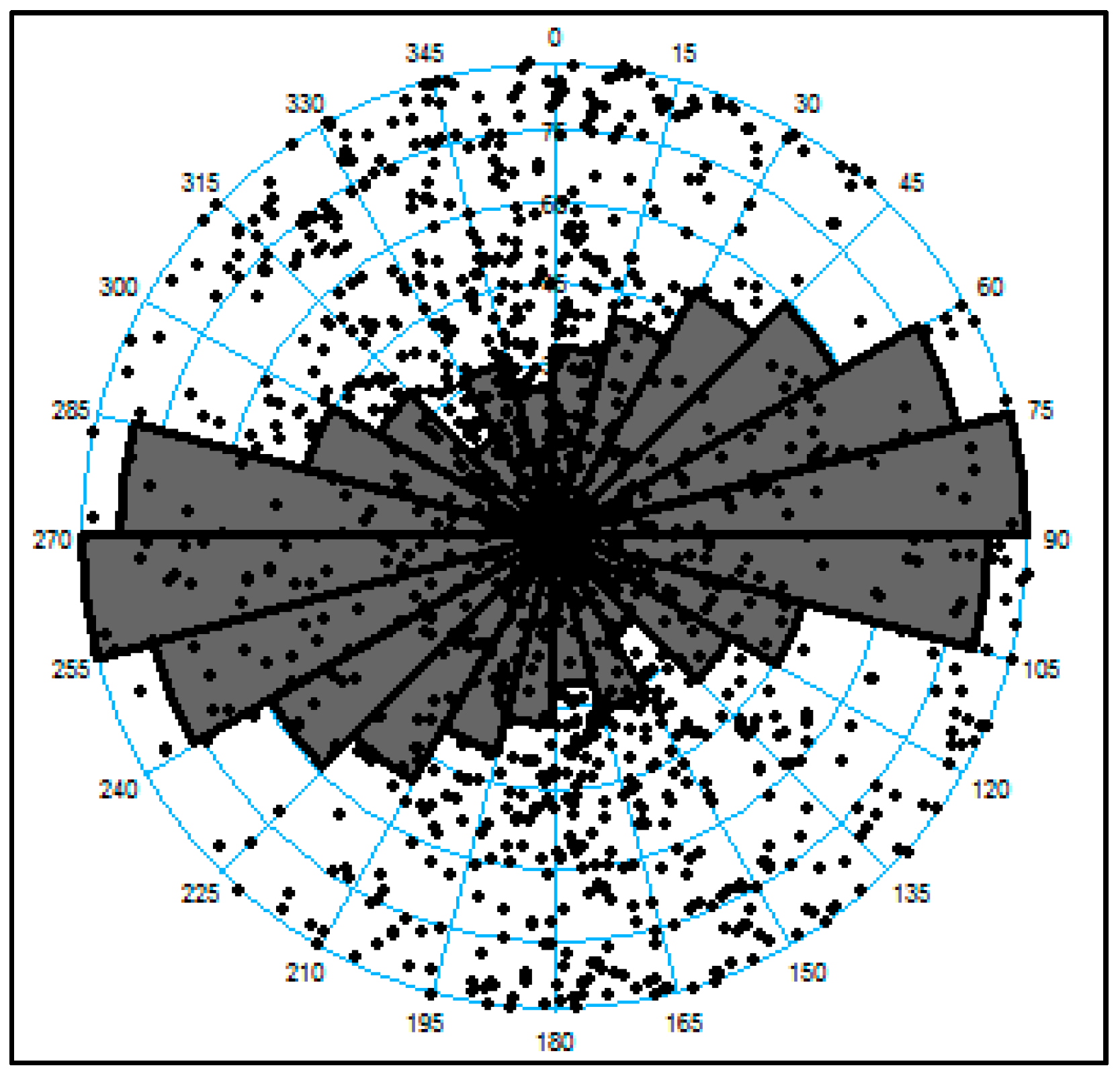
- In total, 1264 subtle faults and LSFs were extracted in the reservoir. These fractures can be divided into two sets in terms of the azimuth distribution. Mostly, the strike of the fractures is in the W–E direction;
- (4)
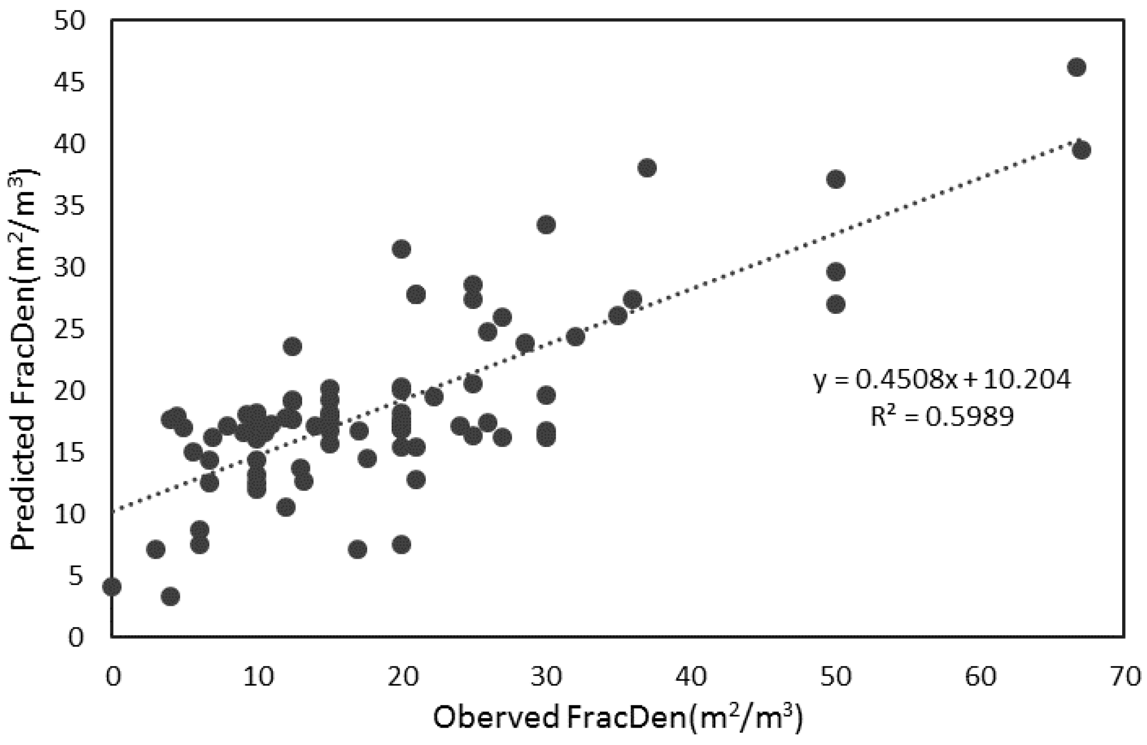
- The fracture density is predicted through an integrated method by combining the core observation, well log interpretation, and artificial neural network algorithm. The spatial distribution of the fractures matched the faults.
Acknowledgments
Author Contributions
Conflicts of Interest
References
- Nelson, R.A. Geologic Analysis of Naturally Fractured Reservoirs, 2nd ed.; Gulf Professional Publishing: Huston, TX, USA, 2001. [Google Scholar]
- Boro, H.; Rosero, E.; Bertotti, G. Fracture-network analysis of the Latemar Platform (northern Italy): Integrating outcrop studies to constrain the hydraulic properties of fractures in reservoir models. Pet. Geosci. 2014, 20, 79–92. [Google Scholar] [CrossRef]
- Wennberg, O.P.; Casini, G.; Jonoud, S.; Peacock, D.C.P. The characteristics of open fractures in carbonate reservoirs and their impact on fluid flow: A discussion. Pet. Geosci. 2016, 22, 91–104. [Google Scholar] [CrossRef]
- Nasseri, A.; Mohammadzadeh, M.J.; Raeisi, H.T. Fracture enhancement based on artificial ants and fuzzy c-means clustering (FCMC) in Dezful Embayment of Iran. J. Geophys. Eng. 2015, 12, 227–241. [Google Scholar] [CrossRef]
- Deng, X.L.; Li, J.H.; Liu, L.; Ren, K.X. Advances in the study of fractured reservoir characterization and modelling. Geol. J. China Univ. 2015, 21, 306–319. [Google Scholar]
- Basir, H.M.; Javaherian, A.; Yaraki, M.T. Multi-attribute ant-tracking and neural network for fault detection: A case study of an Iranian oilfield. J. Geophys. Eng. 2013, 10, 1–10. [Google Scholar] [CrossRef]
- Chopra, S.; Marfurt, K.J. Volumetric curvature attributes for fault/fracture characterization. First Break 2007, 25, 35–46. [Google Scholar] [CrossRef]
- Dalley, R.M.; Gevers, E.E.A.; Stampli, G.M.; Davies, D.J.; Gastaldi, C.; Ruijter, P.R.; Vermeer, G. Dip and azimuth displays for 3-D seismic interpretation. First Break 1989, 7, 86–95. [Google Scholar] [CrossRef]
- Rijks, E.J.H.; Jauffred, J.C.E.M. Attribute extraction: An important application in any detailed 3-D interpretation study. Lead. Edge 1991, 10, 9–11. [Google Scholar] [CrossRef]
- Roberts, A. Curvature attributes and their application to 3D interpreted horizons. First Break 2001, 19, 85–100. [Google Scholar] [CrossRef]
- Hart, B.S.; Pearson, R.; Rawling, G.C. 3D seismic horizon-based approaches to fracture-swarm sweet spot definition in tight-gas reservoirs. Lead. Edge 2002, 21, 28–35. [Google Scholar] [CrossRef]
- Al-Dossary, S.; Marfurt, K.J. 3D volumetric multispectral estimates of reflector curvature and rotation. Geophysics 2006, 71, 41–51. [Google Scholar] [CrossRef]
- Luis, B.; Milagrosa, A. Volume curvature attributes to identify subtle faults and fractures in carbonate reservoirs: Cimarrona Formation, Middle Magdalena Valley Basin, Colombia. In Proceedings of the SEG Denver 2010 Annual Meeting, Denver, CO, USA, 17–22 October 2010.
- Bahorich, M.S.; Farmer, S.L. 3D seismic discontinuity for faults and stratigraphic features: The coherence cube. Lead. Edge 1995, 14, 1053–1058. [Google Scholar] [CrossRef]
- Marfurt, K.J.; Kirlin, R.L.; Farmer, S.H.; Bahorich, M.S. 3D seismic attributes using a semblance-based algorithm. Geophysics 1998, 63, 1150–1165. [Google Scholar] [CrossRef]
- Gresztenkorn, A.; Marfurt, K.J. Eigenstructure-based coherence computations as an aid to 3D structural and stratigraphic mapping. Geophysics 1999, 64, 1468–1479. [Google Scholar] [CrossRef]
- Silva, C.C.; Marcolino, C.S.; Lima, F.D. Automatic fault extraction using ant tracking algorithm in the Marlim South Filed, Campos Basin. In Proceedings of the 9th International Congress of the Brazilian Geophysical Society, Extended Abstracts, Salvador, Brazil, 11–14 September 2005; pp. 857–860.
- Ngeri, A.P.; Tamunobereton-ari, I.; Amakiri, A.R.C. Ant-tracker attributes: An effective approach to enhancing fault identification and interpretation. IOSR J. VLSI Signal Process. 2015, 5, 67–73. [Google Scholar]
- Baytok, S.; Pranter, M.J. Fault and fracture distribution within a tight-gas sandstone reservoir: Mesaverde Group, Mamm Creek Field, Piceance Basin, Colorado, USA. Pet. Geosci. 2013, 19, 203–222. [Google Scholar] [CrossRef]
- Noha, S.F.; Mark, D.Z. Utilizing ant-tracking to identify slowly slipping faults in the Barnett Shale. In Proceedings of the Unconventional Resources Technology Conference, Denver, CO, USA, 25–27 August 2014.
- Ahmadi, M.A.; Zendehboudi, S.; Lohi, A.; Elkamel, A.; Chatzis, I. Reservoir permeability prediction by neural networks combined with hybrid genetic algorithm and particle swarm optimization. J. Geophys. Prospect. 2013, 61, 582–598. [Google Scholar] [CrossRef]
- Zendehboudi, S.; Ahmadi, M.A.; Bahadori, A.; Shafiei, A.; Babadaghli, T. A developed smart technique to predict minimum miscible pressure—EOR implications. Can. J. Chem. Eng. 2012, 91, 1325–1337. [Google Scholar] [CrossRef]
- Zendehboudi, S.; Ahmadi, M.A.; James, L.; Chatzis, I. Prediction of condensate-to-gas ratio for retrograde gas condensate reservoirs using artificial neural network with particle swarm optimization. Energy Fuels 2012, 26, 3432–3447. [Google Scholar] [CrossRef]
- Shafiei, A.; Dusseault, M.B.; Zendehboudi, S.; Chatzis, I. A new screening tool for evaluation of steamflooding performance in naturally fractured carbonate heavy oil reservoirs. Fuel 2013, 108, 502–514. [Google Scholar] [CrossRef]
- Liu, Y.; Dong, N.; Fehler, M.; Fang, X.; Liu, X. Estimating the fracture density of small-scale vertical fractures when large-scale vertical fractures are present. J. Geophys. Eng. 2015, 12, 311–320. [Google Scholar] [CrossRef]
- Lefranc, M.; Farag, S.; Souche, L.; Dubois, A. Fractured basement reservoir characterization for fracture distribution, porosity and permeability prediction. In Proceedings of the AAPG International Conference and Exhibition, Singapore, 16–19 September 2012.
- Schlumberger. High-Definition Formation Microimager, 2013. Available online: http//www.slb.com/fmi-hd (accessed on 23 November 2016).
- Weatherford. Compact Microimager, 2013. Available online: http://www.weatherford.com/doc/wft268562 (accessed on 23 November 2016).
- Al-Anazi, A.; Babadagli, T. Automatic fracture density update using smart well data and artificial neural networks. Comput. Geosci. 2010, 36, 335–347. [Google Scholar] [CrossRef]
- Tokhmchi, B.; Memarian, H.; Rezaee, M.R. Estimation of the fracture density in fractured zones using petrophysical logs. J. Pet. Sci. Eng. 2010, 72, 206–213. [Google Scholar] [CrossRef]
- Zazoun, R.S. Fracture density estimation from core and conventional well logs data using artificial neural networks: The Cambro-Ordovician reservoir of Mesdar oil field, Algeria. J. Afr. Earth Sci. 2013, 83, 55–73. [Google Scholar] [CrossRef]
- Jafari, A.; Babadagli, T. Estimation of equivalent fracture network permeability using fractal and statistical network properties. J. Pet. Sci. Eng. 2012, 92–93, 110–123. [Google Scholar] [CrossRef]
- Walter, H.F.; Dresser, A. Evaluation of fractured reservoir rocks using geophysical well logs. In Proceedings of the SPE Unconventional Gas Recovery Symposium, Pittsburgh, PA, USA, 18–21 May 1980.
- Martinez, L.P. Characterization of Naturally Fractured Reservoirs from Conventional Well Logs. Master’s Thesis, University of Oklahoma, Norman, OK, USA, 2002. [Google Scholar]
- Caers, J. Petroleum Geostatistics; Society of Petroleum Engineers: Richardson, TX, USA, 2005. [Google Scholar]
- Zhou, F.; Allinson, G.; Wang, J.; Sun, Q.; Xiong, D.; Cinar, Y. Stochastic modelling of coalbed methane resources: A case study in Southeast Qingshui Basin, China. Int. J. Coal Geol. 2012, 99, 16–26. [Google Scholar] [CrossRef]
- Barenblatt, G.I.; Zheltov, Y.P. Fundamental equations of filtration of homogeneous liquids in fissured rocks. Dokl. Akad. Nauk SSSR 1960, 13, 545–548. [Google Scholar]
- Warren, J.E.; Root, P.J. The behaviour of naturally fractured reservoirs. SPE J. 1963, 3, 245–255. [Google Scholar] [CrossRef]
- Kazemi, H.; Merrill, L.S.; Porterfield, K.L. Numerical simulation of water-oil flow in naturally fractured reservoirs. SPE J. 1976, 16, 317–326. [Google Scholar] [CrossRef]
- Thomas, L.K.; Dixon, T.N.; Pierson, R.G. Fractured reservoir simulation. SPE J. 1983, 23, 42–54. [Google Scholar] [CrossRef]
- Dai, Z.X.; Wolfsberg, A.; Lu, Z.M.; Reimus, P. Upscaling matrix diffusion coefficients for heterogeneous fractured rocks. Geophys. Res. Lett. 2007, 34. [Google Scholar] [CrossRef]
- Pedersen, S.I.; Skov, T.; Hetlelid, A.; Fayemendy, P.; Randen, T.; Sonneland, L. New paradigm of fault interpretation. SEG Tech. Program Expand. Abstr. 2003. [Google Scholar] [CrossRef]
- Pointe, L. A workflow for building and validation static reservoir models for fractured reservoirs for direct implementation into Dynamic Simulators. In Proceedings of the AAPG Annual Meeting, Dallas, TX, USA, 18–21 April 2004.
- Cherpeau, N.; Caumon, G. Stochastic structural modelling in sparse data situations. Pet. Geosci. 2015, 21, 233–247. [Google Scholar] [CrossRef]
- Wang, X.N.; Ghassemi, A. A three-dimensional stochastic fracture network model for geothermal reservoir simulation. In Proceedings of the Thirty-Sixth Workshop on Geothermal Reservoir Engineering, Stanford, CA, USA, 31 January–2 February 2011.
- Oda, M. Permeability tensor for discontinuous rock mass. Geotechnique 1985, 35, 483–495. [Google Scholar] [CrossRef]
- Dai, Z.; Wolfsberg, A.; Lu, Z.; Deng, H. Scale dependence of sorption coefficients for contaminant transport in saturated fractured rock. Geophys. Res. Lett. 2009, 36, L01403. [Google Scholar] [CrossRef]
- Ampomah, W.; Balch, R.; Cather, M.; Rose-Coss, D.; Dai, Z.; Heath, J.; Dewers, T.; Mozley, P. Evaluation of CO2 Storage Mechanisms in CO2 Enhanced Oil Recovery Sites: Application to Morrow Sandstone Reservoir. Energy Fuels 2016, 30, 8545–8555. [Google Scholar] [CrossRef]
- Shan, Y.; Ge, W. A preliminary stugy on the Formation Mechanisms of natural fractures in reservoirs: An Example from Jingbei Buried-hill Pool, North of Central Liaoning Province. Pet. Geol. Exp. 2001, 23, 457–464. [Google Scholar]
- Zeng, L.; Zhang, J.; Zhang, Y. The study of fissures development in Jingbei buried hill reservoir in Liaohe Basin. China Offshore Oil Gas 1998, 12, 381–385. [Google Scholar]
- Shan, Y.; Ge, W. Fracture pattern of middle Proterozoic in Jingbei buried hill, central Liaoning province. Pet. Explor. 1997, 2, 37–42. [Google Scholar]
- Ni, G.; Bao, Z.; Du, X.; Zhang, Z.; Li, X.; Chen, S. Bedrock reservoir of Jingbei buried hill in Damintun Sag, Liaohe Depression. Pet. Explor. Dev. 2006, 33, 461–465. [Google Scholar]
- Shan, Y.; Ge, W. Minor Fault Simulation in Jingbei Buried-hill Reservoir. Pet. Explor. Dev. 1998, 25, 80–83. [Google Scholar]
- Randen, T.; Peldersen, S.I.; Sønneland, L. Automatic extraction of fault surfaces from three-dimensional seismic data. Seg Technical Program Expanded Abstracts. In Proceedings of the SEG Int’l Exposition and Annual Meeting, San Antonio, TX, USA, 9–14 September 2001.
- Petrel. In Petrel Help Center; Schlumberger: Houston, TX, USA, 2014.
- Zhao, J.; Sun, S.Z. Automatic fault extraction using a modified ant-colony algorithm. J. Geophys. Eng. 2013, 10, 1–7. [Google Scholar] [CrossRef]
- Jafari, A.; Kadkhodaie-Ilkhchi, A.; Sharghi, Y.; Ghanavati, K. Fracture density estimation from petrophysical log data using the adaptive neuro-fuzzy inference system. J. Geophys. Eng. 2012, 9, 105–114. [Google Scholar] [CrossRef]
- Nikravesh, M. Soft computing-based computational intelligent for reservoir characterization. Expert Syst. Appl. 2004, 26, 19–38. [Google Scholar] [CrossRef]
- Wikipedia. Overfitting. 2017. Available online: https://www.en.wikipedia.org/wiki/Overfitting (accessed on 1 November 2016).
- Malin, P.; Leary, P.; Shalev, E.; Rugis, J.; Valles, B.; Boes, C.; Andrews, J.; Geiser, P. Flow lognormality and spatial correlation in crustal reservoirs: II-where-to-drill guidance via acoustic/seismic imaging. In Proceedings of the World Geothermal Congress, Melbourne, Australia, 19–25 April 2015.


| Structural Smoothing | Filter option | Sigma X | Sigma Y | Sigma Z |
| Plain | 1.5 | 1.5 | 1.5 | |
| Variance | Inline range | Crossline range | Vertical smoothing | Plane confidence threshold |
| 3 | 3 | 15 | 0.9 | |
| 3D Edge Enhancement | Horizontal/Vertical radius | Plane half thickness | Minimum/Maximum dip | Maximum/Maximum strike |
| 5/10 | 10 | 50/90 | 0/180 |
| Initial Ant Boundary | Ant Track Deviation | Ant Step Size | Illegal Steps Allowed | Legal Steps Required | Stop Criteria |
|---|---|---|---|---|---|
| 5 | 2 | 3 | 2 | 2 | 10 |
| Extraction Sampling Distance | Extraction Sampling Threshold | Extraction Background Threshold | Deviation from a Plane | Connectivity Constraint | Minimum Patch Size | Patch Down Sampling |
|---|---|---|---|---|---|---|
| 6 voxels | Top 60% | Top 80% | 7 voxels | 2 faces | 50 points | 8 voxels |
| AC, μs/m | GR, API | CN, % | DEN, g/cm3 | Ant Tracking | Frac Density, m2/m3 |
|---|---|---|---|---|---|
| 183.99 | 21.25 | 15.00 | 2.68 | 0.08 | 0.0 |
| 187.63 | 18.89 | 14.32 | 2.78 | 0.08 | 3.0 |
| 179.11 | 20.53 | 17.68 | 2.70 | 0.08 | 4.0 |
| 136.47 | 6.91 | 3.99 | 2.82 | 0.00 | 4.0 |
| 157.72 | 2.02 | 5.00 | 2.75 | 0.00 | 4.5 |
| 148.89 | 4.49 | 6.22 | 2.81 | 0.15 | 4.9 |
| 171.32 | 13.13 | 7.20 | 2.72 | 0.00 | 5.6 |
| 208.47 | 19.97 | 14.64 | 2.68 | 0.08 | 6.0 |
| 188.00 | 14.81 | 20.00 | 2.68 | –0.01 | 6.1 |
| 132.42 | 1.95 | 2.00 | 2.79 | 0.49 | 6.7 |
| 124.02 | 3.12 | 1.00 | 2.77 | 0.47 | 6.7 |
| 143.08 | 3.78 | 4.76 | 2.84 | 0.19 | 7.0 |
| 156.68 | 4.07 | 4.92 | 2.78 | 0.20 | 8.0 |
| 145.50 | 3.99 | 8.99 | 2.84 | 0.15 | 9.1 |
| 183.13 | 4.65 | 4.68 | 2.86 | 0.00 | 9.3 |
| 182.41 | 14.22 | 14.64 | 2.65 | 0.02 | 10.0 |
| 184.59 | 20.18 | 13.00 | 2.74 | 0.24 | 10.0 |
| 164.21 | 12.68 | 10.64 | 2.73 | –0.01 | 10.0 |
| 250.26 | 18.12 | 14.32 | 2.61 | 0.09 | 10.0 |
| 142.54 | 3.33 | 7.32 | 2.84 | 0.20 | 10.0 |
| 155.59 | 4.26 | 5.90 | 2.77 | 0.19 | 10.0 |
| 156.11 | 4.81 | 6.87 | 2.80 | 0.22 | 10.0 |
| 162.62 | 5.45 | 9.15 | 2.74 | 0.01 | 10.0 |
| 149.93 | 8.77 | 3.20 | 2.80 | 0.00 | 10.0 |
| 164.08 | 7.96 | 13.94 | 2.67 | 0.00 | 10.2 |
| 155.08 | 6.16 | 7.38 | 2.80 | 0.00 | 10.2 |
| 157.13 | 6.17 | 12.10 | 2.76 | 0.00 | 10.6 |
| 145.28 | 4.62 | 8.40 | 2.73 | 0.01 | 11.0 |
| 210.32 | 18.39 | 13.00 | 2.69 | 0.08 | 12.0 |
| 159.27 | 4.53 | 9.60 | 2.72 | 0.00 | 12.0 |
| 187.63 | 10.94 | 5.00 | 2.80 | 0.03 | 12.5 |
| 187.26 | 8.52 | 3.00 | 2.80 | 0.03 | 12.5 |
| 177.23 | 6.41 | 6.00 | 2.70 | 0.01 | 12.5 |
| 238.67 | 6.68 | 11.00 | 2.60 | 0.01 | 12.5 |
| 203.92 | 12.69 | 23.00 | 2.63 | 0.02 | 13.0 |
| 178.06 | 16.12 | 20.00 | 2.83 | 0.19 | 13.3 |
| 146.62 | 4.04 | 6.33 | 2.80 | –0.01 | 14.0 |
| 180.72 | 4.36 | 2.00 | 2.77 | 0.51 | 15.0 |
| 147.59 | 4.12 | 5.26 | 2.81 | 0.19 | 15.0 |
| 160.44 | 5.18 | 7.80 | 2.79 | 0.00 | 15.0 |
| 158.78 | 4.89 | 2.68 | 2.87 | 0.00 | 15.0 |
| 159.06 | 3.22 | 2.51 | 2.68 | 0.16 | 15.0 |
| 176.45 | 3.99 | 4.91 | 2.68 | 0.14 | 15.0 |
| 208.59 | 9.96 | 2.00 | 2.77 | 0.01 | 15.0 |
| 193.97 | 20.00 | 13.32 | 2.71 | 0.08 | 17.0 |
| 149.34 | 5.77 | 9.26 | 2.77 | 0.00 | 17.1 |
| 174.57 | 1.75 | 3.00 | 2.77 | 0.33 | 17.6 |
| 204.09 | 20.21 | 18.68 | 2.57 | 0.09 | 20.0 |
| 193.13 | 14.77 | 9.68 | 2.69 | 0.09 | 20.0 |
| 155.68 | 5.55 | 11.36 | 2.75 | 0.00 | 20.0 |
| 138.01 | 5.61 | 6.00 | 2.82 | 0.00 | 20.0 |
| 136.94 | 3.13 | 4.56 | 2.78 | 0.00 | 20.0 |
| 136.91 | 5.01 | 5.56 | 2.79 | 0.00 | 20.0 |
| 140.31 | 5.50 | 5.00 | 2.83 | 0.00 | 20.0 |
| 145.70 | 4.99 | 4.88 | 2.79 | 0.16 | 20.0 |
| 155.75 | 8.65 | 5.78 | 2.74 | 0.00 | 20.0 |
| 148.90 | 6.04 | 5.25 | 2.77 | 0.23 | 20.0 |
| 180.68 | 7.00 | 9.00 | 2.63 | 0.08 | 20.0 |
| 213.38 | 9.82 | 6.00 | 2.70 | 0.08 | 20.0 |
| 309.26 | 2.84 | 5.36 | 2.61 | 0.08 | 20.0 |
| 177.83 | 16.00 | 10.00 | 2.75 | 0.08 | 21.0 |
| 160.02 | 12.37 | 7.68 | 2.77 | 0.04 | 21.0 |
| 284.19 | 4.96 | 0.00 | 2.63 | 0.11 | 21.0 |
| 288.12 | 12.52 | 0.68 | 2.60 | 0.08 | 21.0 |
| 183.15 | 1.74 | 5.00 | 2.73 | 0.00 | 22.2 |
| 144.95 | 5.21 | 5.23 | 2.85 | 0.09 | 24.0 |
| 142.33 | 4.47 | 9.55 | 2.81 | 0.00 | 25.0 |
| 201.62 | 4.37 | 8.32 | 2.69 | 0.08 | 25.0 |
| 264.01 | 8.80 | 0.00 | 2.60 | 0.08 | 25.0 |
| 276.55 | 6.55 | 0.00 | 2.60 | 0.08 | 25.0 |
| 153.85 | 5.47 | 9.22 | 2.72 | –0.01 | 26.0 |
| 218.58 | 5.74 | 0.00 | 2.59 | 0.08 | 26.0 |
| 146.41 | 3.09 | 3.44 | 2.84 | 0.14 | 27.0 |
| 267.75 | 5.16 | 0.00 | 2.62 | 0.16 | 27.0 |
| 295.85 | 10.14 | 6.00 | 2.75 | 0.08 | 28.6 |
| 137.74 | 3.90 | 8.98 | 2.84 | 0.09 | 30.0 |
| 139.41 | 5.58 | 8.34 | 2.79 | 0.00 | 30.0 |
| 150.62 | 3.56 | 5.04 | 2.79 | 0.17 | 30.0 |
| 201.07 | 4.04 | 2.00 | 2.83 | 0.00 | 30.0 |
| 339.43 | 10.96 | 0.00 | 2.59 | 0.08 | 30.0 |
| 212.00 | 1.50 | 0.00 | 2.63 | 0.00 | 32.0 |
| 207.72 | 1.70 | 0.00 | 2.55 | 0.00 | 35.0 |
| 264.00 | 8.84 | 0.00 | 2.60 | 0.08 | 36.0 |
| 265.40 | 4.99 | 4.96 | 2.22 | 0.08 | 37.0 |
| 251.27 | 6.35 | 0.00 | 2.59 | 0.08 | 50.0 |
| 275.64 | 1.64 | 2.00 | 2.56 | 0.08 | 50.0 |
| 207.06 | 15.30 | 7.00 | 2.60 | 0.76 | 50.0 |
| 251.88 | 15.84 | 23.00 | 2.72 | 0.72 | 66.7 |
| 222.32 | 15.60 | 19.00 | 2.63 | 0.63 | 67.0 |
| Fracture Set | Mean Dip, Degree | Mean Azimuth, Degree | Concentration | Anisotropy | Statistical Method |
|---|---|---|---|---|---|
| Fracture set 1 | 37.0 | 166.7 | 2.5 | 0.1 | Kent model |
| Fracture set 2 | 36.7 | 346.4 | 2.6 | 0.1 | Kent model |
© 2017 by the authors. Licensee MDPI, Basel, Switzerland. This article is an open access article distributed under the terms and conditions of the Creative Commons Attribution (CC BY) license ( http://creativecommons.org/licenses/by/4.0/).
Share and Cite
Fang, J.; Zhou, F.; Tang, Z. Discrete Fracture Network Modelling in a Naturally Fractured Carbonate Reservoir in the Jingbei Oilfield, China. Energies 2017, 10, 183. https://doi.org/10.3390/en10020183
Fang J, Zhou F, Tang Z. Discrete Fracture Network Modelling in a Naturally Fractured Carbonate Reservoir in the Jingbei Oilfield, China. Energies. 2017; 10(2):183. https://doi.org/10.3390/en10020183
Chicago/Turabian StyleFang, Junling, Fengde Zhou, and Zhonghua Tang. 2017. "Discrete Fracture Network Modelling in a Naturally Fractured Carbonate Reservoir in the Jingbei Oilfield, China" Energies 10, no. 2: 183. https://doi.org/10.3390/en10020183