Investigating How an Artificial Neural Network Model Can Be Used to Detect Added Mass on a Non-Rotating Beam Using Its Natural Frequencies: A Possible Application for Wind Turbine Blade Ice Detection

Abstract

Structures vibrate with their natural frequencies when disturbed from their equilibrium position. These frequencies reduce when an additional mass accumulates on their structures, like ice accumulation on wind turbines installed in cold climate sites. The added mass has two features: the location and quantity of mass. Natural frequencies of the structure reduce differently depending on these two features of the added mass. In this work, a technique based on an artificial neural network (ANN) model is proposed to identify added mass by training the neural network with a dataset of natural frequencies of the structure calculated using different quantities of the added mass at different locations on the structure. The proposed method is demonstrated on a non-rotating beam model fixed at one end. The length of the beam is divided into three zones in which different added masses are considered, and its natural frequencies are calculated using a finite element model of the beam. ANN is trained with this dataset of natural frequencies of the beam as an input and corresponding added masses used in the calculations as an output. ANN approximates the non-linear relationship between these inputs and outputs. An experimental setup of the cantilever beam is fabricated, and experimental modal analysis is carried out considering a few added masses on the beam. The frequencies estimated in the experiments are given as an input to the trained ANN model, and the identified masses are compared against the actual masses used in the experiments. These masses are identified with an error that varies with the location and the quantity of added mass. The reason for these errors can be attributed to the unaccounted stiffness variation in the beam model due to the added mass while generating the dataset for training the neural network. Therefore, the added masses are roughly estimated. At the end of the paper, an application of the current technique for detecting ice mass on a wind turbine blade is studied. A neural network model is designed and trained with a dataset of natural frequencies calculated using the finite element model of the blade considering different ice masses. The trained network model is tested to identify ice masses in four test cases that considers random mass distributions along the blade. The neural network model is able to roughly estimate ice masses, and the error reduces with increasing ice mass on the blade.

1. Introduction

Wind turbine installations in the northeastern and mid-Atlantic U.S., Canada, Northern Europe and other high altitude areas are increasing due to good wind resources. Cold and humid weather conditions in these sites in winters increase the risk of ice accretion on wind turbines. Ice accumulates on the wind turbine blades when moisture in the air impacts the cold surface of the blades. The amount of ice accretion depends on various parameters, like ambient temperature, the moisture content of the air, wind velocity and the duration of the icing event. The global wind energy installations in cold climate regions reached a capacity of 127 GW at the end of 2015, and the forecast is that it would reach a capacity of 186 GW by the end of 2020 [1]. Icing of the rotor blades results in reduced turbine power output as icing reduces the lift force and increases the drag force [2,3]. Additionally, nacelle vibration amplitudes increase during the icing conditions, so icing can be detected more reliably using the power curve analysis along with nacelle vibration analysis [4]. Etemaddar et al. [5] investigated the effects of atmospheric ice accumulation on the aerodynamic performance and structural response of a wind turbine, and they predicted that the relative change in mean value is bigger than the change in standard deviation for most of the response quantities (rotor speed, torque, power, thrust and structural loads) of the iced blade. Alsabagh et al. [6] considered different ice mass distributions as defined in the ISO 12494:2001 standard on a multi megawatt wind turbine blade. They analyzed the influences of ice mass on natural frequencies and dynamic magnification factors (ratio of the dynamic deflection to static deflection), by considering only the mass changes in the blade. Gantasala et al. [7] analyzed the modal behavior of a 2-MW wind turbine blade under icing conditions. Their analysis showed that the aeroelastic damping factors of the vibration modes reduce when ice accumulates on the blade.

Icing causes measurement errors in the instruments, reduces turbine power output, increases vibrations and loads in the mechanical components and increases the noise and safety risks of ice shedding [8]. Turbine manufacturers are working on technologies to prevent ice formation on the blades, known as anti-icing methods, and ice removal using hot air or heating resistance, known as de-icing methods. For efficient operation of these systems, ice formation needs to be detected in the early stages so that the losses due to blade icing can be minimized and also de-icing of the blades can be performed with less external power. This requires a reliable technique to detect the location and quantity of ice mass on the blades. An ideal de-icing system can be designed with such a technique to automatically stop the turbine and remove ice once an icing event is detected, which will eliminate the need of physical inspection by the turbine maintenance personnel.

Homola et al. [9] investigated 29 different ice sensors and concluded that no sensor performs satisfactorily in different conditions arising in turbine operation. The ice detection sensors can be broadly divided into nacelle- and blade-based systems, and some of these systems are evaluated in [10]. The main disadvantage with nacelle-based systems is that they detect ice based on the operating conditions existing at the nacelle height. In the case of larger wind turbine blades, nacelle-based systems cannot identify icing events caused when cloud heights are above or below the nacelle height. Icing in the outer half of the blade reduces power output more, and this portion of the blade generally accumulates more ice as it sweeps through a larger area in rotation and experiences wind at higher relative velocity. Thus, ice detection using sensors installed on the blade near the tip region can reliably and efficiently detect icing.

The increase in blade mass due to the ice accumulation reduces its natural frequencies depending on the quantity of accumulated ice mass and its location along the blade. The ice detection systems, like the BLADEControl system [11,12] and fos4blade IceDetection [10,13], Wolfel IDD.Blade [14], detect ice based on the deviations in blade natural frequencies. These systems detect icing while the turbine is in operation or at a standstill condition, which enables the automatic restart of the turbine once the blades are ice-free after de-icing. These systems indicate the state of icing on the blades, such as ice-free, non-critical ice and critical ice, but cannot identify the location and quantity of ice mass. As the blade natural frequencies change differently with the location and quantity of ice mass, the authors propose an artificial neural network (ANN) model that detects ice mass accumulated in different zones defined along the blade based on its natural frequencies. The ANN can be used to estimate or approximate functions that depend on multiple variables. Function approximation is the task of learning or constructing a function that generates approximately the same outputs from input vectors as the process being modeled, based on available training data [15]. ANNs are widely used in many areas for function approximation and pattern recognition. Their applications in wind energy are mainly focused on wind power forecasting and wind speed prediction, wind turbine power control, identification and evaluation of faults [16]. Khadiri-Yazami et al. [17] used ANN to detect icing events solely from the meteorological data measured on a 200-m met-mast at an icing relevant site in Germany. They trained the network with measured data of temperature, wind velocity, relative humidity and the existence of liquid water content in the air as inputs and events like icing or no-icing using the data from ice sensors as outputs. The trained network is able to detect icing events accurately for the inputs of some data measured in the same site other than the data used to train the network. This application belongs to the category of pattern recognition using ANN.

In this work, the ice mass detection technique based on a neural network model is demonstrated on a non-rotating cantilever beam. The vibrations of the beam are modeled using the finite element method (FEM), and its natural frequencies are calculated from the eigenvalue analysis of the resulting equations of motion (EOM). The cantilever beam’s length is divided into three zones, and different added masses are considered along these zones to calculate its natural frequencies using the FEM model. The dataset of beam natural frequencies and corresponding added masses considered in the calculations are used to train the ANN. Later, the trained neural network model is used to identify added masses corresponding to natural frequencies estimated from experimental modal analysis of the beam with some added masses. After that, a study is carried out using the current detection technique to identify ice mass on a 2-MW wind turbine blade.

2. Experimental Setup and Modal Analysis

A cantilever beam as shown in Figure 1 is fabricated, whose dimensions and material properties are given in

Table 1. Details of the cantilever beam.

Dimensions
Length	0.45	m
Width	0.02	m
Thickness	0.005	m
Material Properties
Young’s modulus	$2.07\times {10}^{11}$	N/m${}^2$
Density	7656	kg/m${}^3$

. An experimental modal analysis is carried out using an impact hammer for exciting beam vibrations in the flap direction and measuring beam vibration accelerations using a single-axis accelerometer. The details of the instruments used in the experimental modal analysis are given in

Table 2. Modal analysis setup details.

Impact hammer	Bruel & Kjaer Type 8206
Accelerometer	Bruel & Kjaer Type 4507
Data acquisition card	NI 9234
Modal analysis software	$DEWESof{t}^{TM}FRF$

.

The frequency response function (FRF) obtained from the experimental modal analysis of the cantilever beam is shown in Figure 2, where three vibration modes of the beam are identified. These vibration modes are well separated from one another. In the vicinity of each resonance, the FRF is dominated by the contribution of that particular mode alone, and the contributions of other vibration modes are negligible [18]. When structural damping only is present in the system, the receptance FRF traces a perfect circle on the Nyquist plane, and modal parameters can be estimated with better accuracy by fitting a circle to the measured FRF [18], as shown in the Figure 3, which is obtained using $DEWESof{t}^{TM}FRF$ [19] for the vibrations measured in the experimental modal analysis.

3. FEM Modeling of the Beam

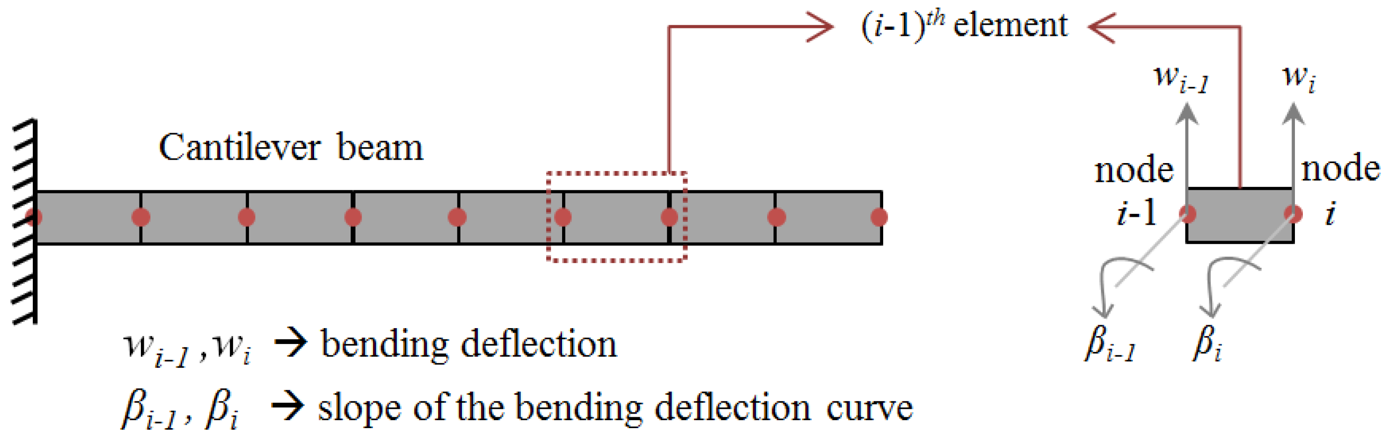
The cantilever beam used in the experimental setup is modeled using Euler beam theory and discretized into finite elements, as shown in the Figure 4. The beam vibrations in vertical plane, i.e., out-of-plane or flap degree of freedom, are only considered in this study. Each element consists of two nodes, and each node has two degrees of freedom. The governing partial differential equations of the beam vibrations given in Equation (1) are analyzed using the finite element method (FEM), and the system matrices of the elements are assembled in the global matrices.

$$\frac{{\partial }^2}{\partial x^2}\left(EI\left(x\right)\frac{{\partial }^{2}w\left(x,t\right)}{\partial x^2}\right)+\rho A\left(x\right)\frac{{\partial }^{2}w\left(x,t\right)}{\partial t^2}=0$$

(1)

where $EI\left(x\right)$ and $\rho A\left(x\right)$ refer to the section stiffness and linear mass density of the beam, respectively; x is the distance of the blade section from the fixed support defined along its length; t refers to the time; $w(x,t)$ refers to the flap vibrations of the beam.

The equations of motion (EOM) obtained from the algebraic equations after discretization are given in Equation (2). One end of the beam is applied fixed boundary conditions in the FEM model.

$$\left[M\right]\left\{\ddot{w}\right\}+\left[K\right]\left\{w\right\}=\left\{0\right\}$$

(2)

where $\left[M\right],\left[K\right]$ refers to the global mass and stiffness matrices of the beam; $\ddot{w}$, w refers to the accelerations and displacements of the vibration degrees of freedom of the beam.

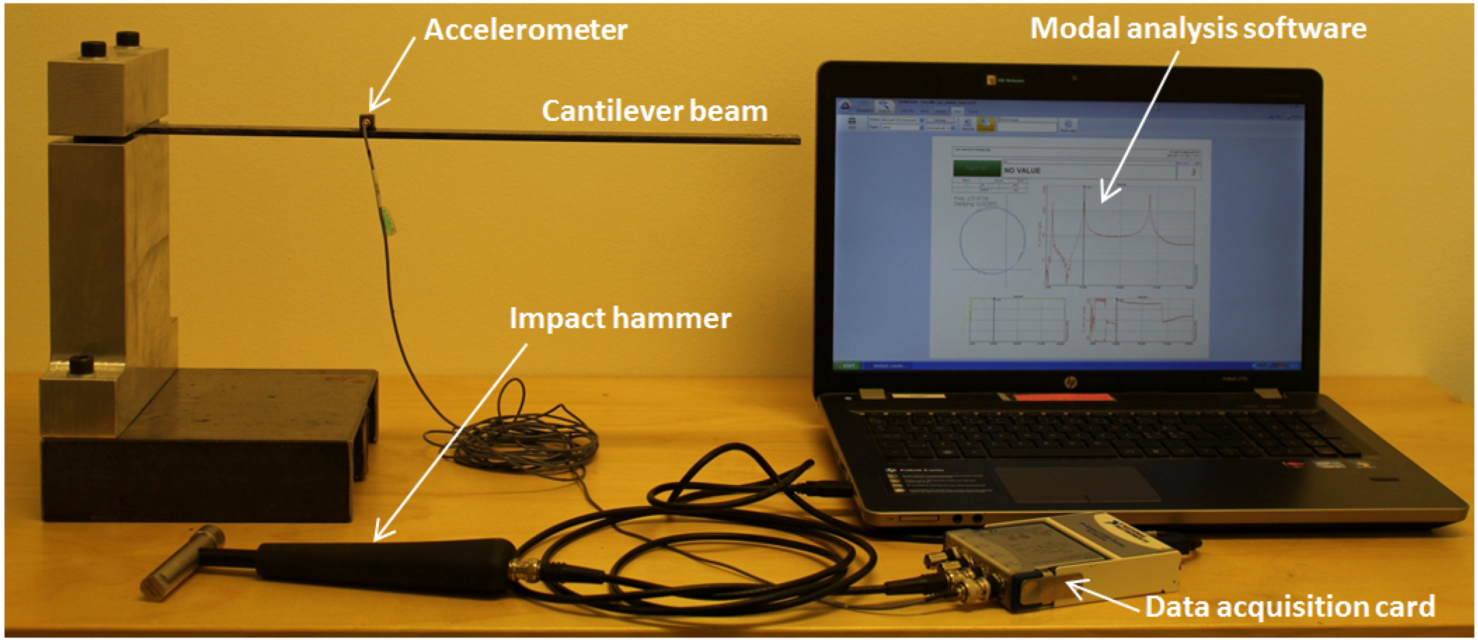
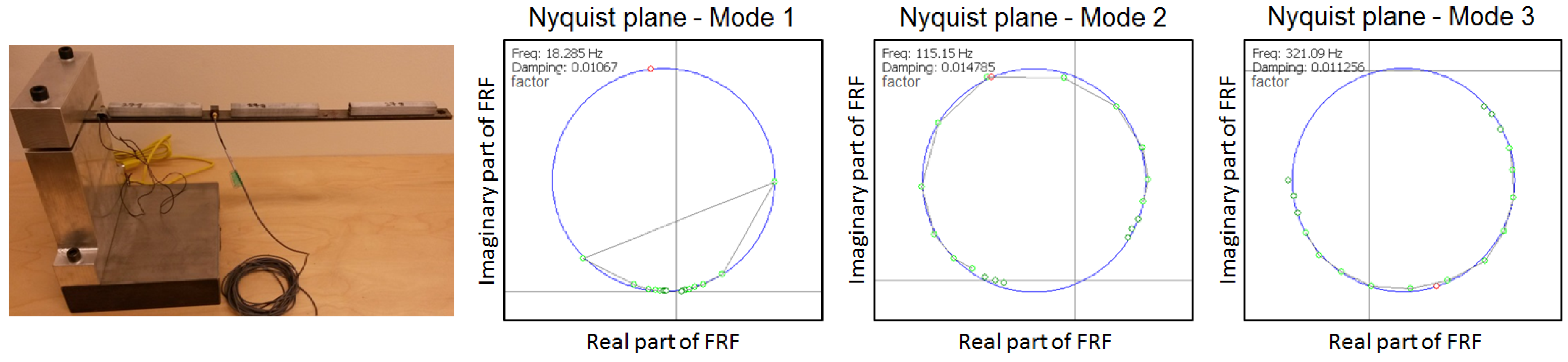
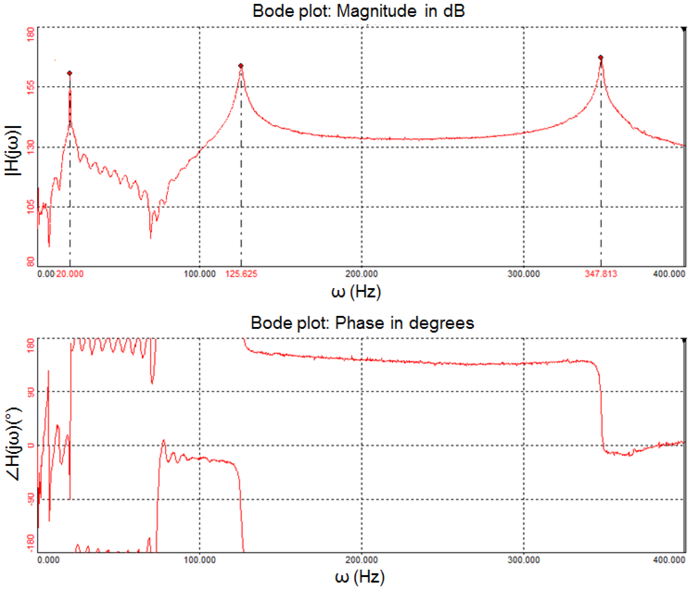
In the experimental setup shown in Figure 1, an accelerometer is placed on the beam at a distance of 0.15 m from its fixed end. The mass of the accelerometer is about 5 g, which is considered as a point mass in the cantilever beam FEM model. As the beam’s cross-section is uniform throughout the length, analytical expressions exist for its natural frequencies if the mass of the accelerometer is ignored. Natural frequencies obtained from the eigenvalue analysis of the EOM are compared with the analytical values and the values estimated from experiments in the

Table 3. Natural frequencies of the cantilever beam.

Vibration Mode	Natural Frequency (Hz)
	Analytical #	FEM (before Updating)	Experiment	FEM (after Updating)
1st Bending	20.74	20.72	20.18	20.26
2nd Bending	129.97	128.68	125.47	125.43
3rd Bending	363.96	358.63	347.97	347.95

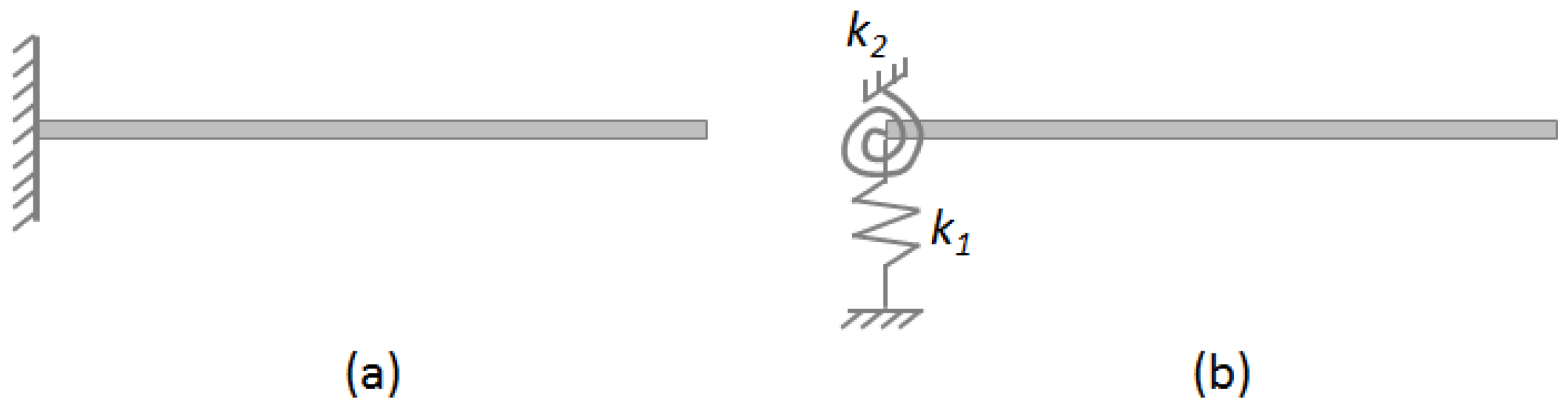
# The mass of the accelerometer is not considered.

. The FEM model’s natural frequencies slightly differ from that of the analytical values due to the mass of the accelerometer. The application of the fixed boundary condition at one end of the beam in the FEM model makes the support infinitely stiff. However, the support used in the experimental setup will have finite stiffness, which is why the frequencies measured in experiments are lower than those calculated using the FEM model. The finite stiffness of the support can be determined using model updating methods [20]. In this study, the support is modeled as two springs with the stiffnesses $k_1,k_2$ as shown in the Figure 5. These stiffness values are added to the global stiffness matrix at the corresponding nodal position in the FEM model. The parameters $k_1,k_2$ are iteratively changed using Equation (3), until the beam natural frequencies calculated from the FEM model closely match with those estimated from experiments. For further details on Equation (3), refer to Sections 2.6 and 8.2 in [21]. The stiffness values of $k_1,k_2$ are found in the model updating process as $5.6995\times {10}^6$ N/m and 8420 Nm/rad. After updating the FEM model with these support stiffnesses, the natural frequencies closely matching with the values estimated from experimental modal analysis as shown in Table 3.

$${\theta }_{j+1}={\theta }_j+{\left[S_j^T{S}_j\right]}^{-1}{S}_j^T\left(z_m-z_j\right)$$

(3)

where ${\theta }_{j+1},{\theta }_j$ are two column vectors of size $2\times 1$ consisting of $k_1,k_2$ values in the $(j+1)$-th and j-th iteration as their elements; $\left[S_j\right]=\frac{\partial {\lambda }_j}{\partial \theta }$ is a $3\times 2$ matrix in the current case (three natural frequencies are chosen to update the FEM model with two support stiffnesses); $\frac{\partial {\lambda }_j}{\partial \theta }={\varphi }_j^T\frac{\partial K}{\partial \theta }{\varphi }_j$, where K is the global stiffness matrix, ${\lambda }_j$ and ${\varphi }_j$ are the eigenvalues and mass normalized eigenvectors, respectively calculated using the FEM model in the j-th iteration; $z_m,z_j$ are two column vectors of size $3\times 1$ consisting of the natural frequencies estimated from the experiments and eigenvalues of the beam FEM model calculated in the j-th iteration, respectively.

4. Artificial Neural Network Model

ANN is a computing system developed using the analogy of biological neural networks that contain a large number of interconnected neurons (nerve cells). The neuron is a small cell that receives electrochemical stimuli (input) from sensory or other types of cells and responds by generating electrical impulses, which will be transmitted to other neurons or effector cells. The same analogy is applied in the ANN models, which use artificial neurons as computing elements for performing some simple computations, and these neurons are interconnected with each other in the network. Each connection within the network is associated with a weight, which either increases or decreases the input signals to the neurons. The neuron behaves as an activation or mapping function (typically a nonlinear function) producing an output corresponding to the input to the neuron. Neural networks can be used for several different kinds of tasks, such as classification, clustering, function approximation and optimization [15]. Each task requires a different kind of network and learning algorithm. The network receives input from the neurons in the input layer, and the output of the network is given by the neurons in the output layer. There may be one or more intermediate hidden layer. Neurons in the network are connected with each other and associated with some weights. These weights are determined in the training process where the relation between input and output variables is determined [16]. The backpropagation algorithm is the most widely-used algorithm to determine the weights of the neurons organized in layers. In this algorithm, the network signal travels in the forward direction, and the errors are propagated backward. The algorithm is provided with a set of inputs and outputs; the error (difference between actual and expected results) is calculated for each input and corresponding output. The backpropagation algorithm is a generalization of the least mean square algorithm that modifies the network weights to minimize the mean square error ($mse$) between the desired and actual outputs of the network. The backpropagation algorithm uses supervised learning in which the network is trained using data for which inputs, as well as desired outputs are known. Once trained, the network weights are frozen and can be used to compute output values for new input samples.

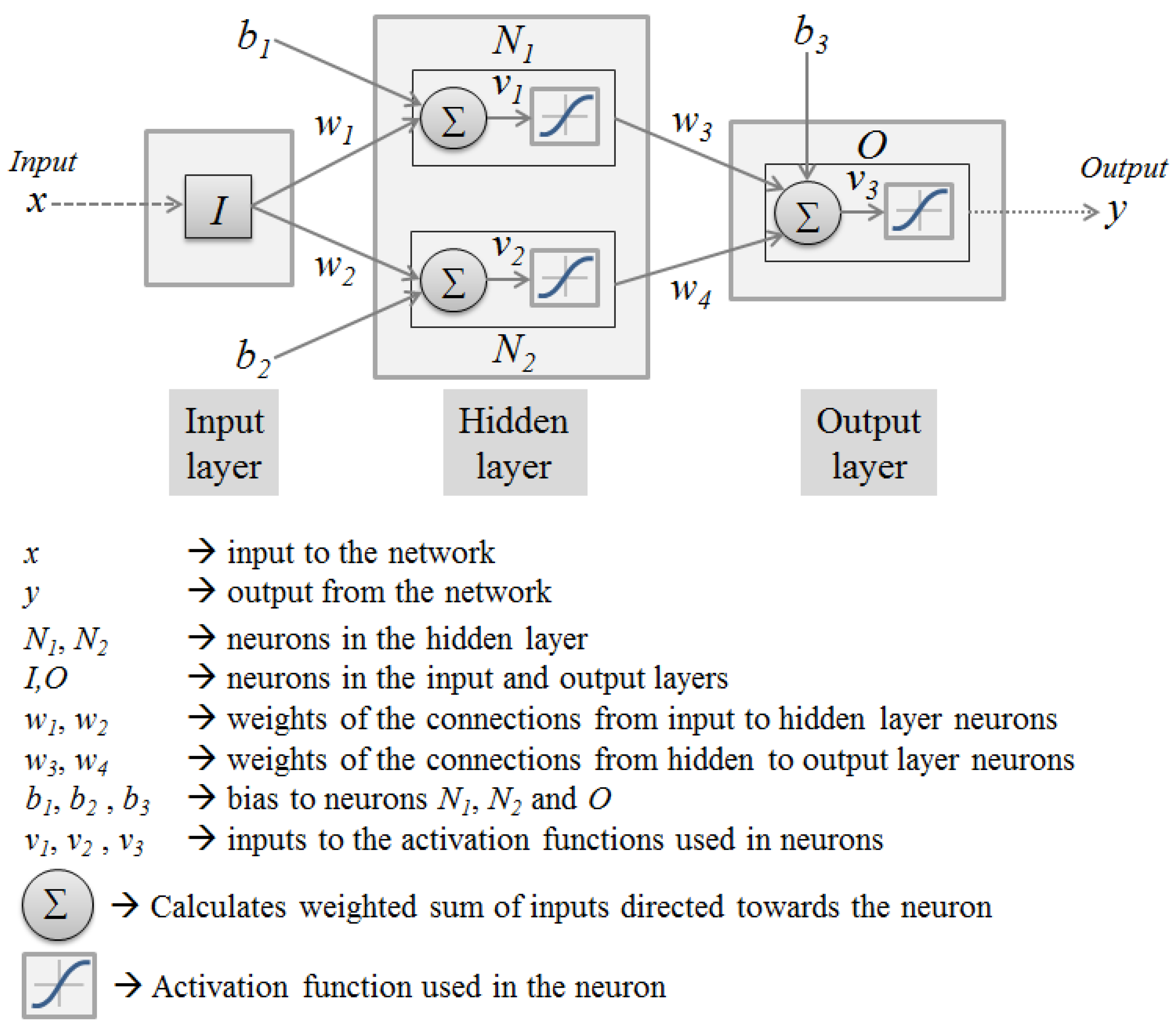
A simple network with two neurons in a hidden layer is shown in Figure 6. The input to the network is x, and the output from the network is y. The connections between neurons from the input to the hidden layer are associated with weights $w_1$, $w_2$, and the neurons in the hidden layer are associated with biases $b_1$, $b_2$. The neurons from the hidden to the output layer are associated with weights $w_3$, $w_4$, and the neuron in the output layer is associated with bias $b_3$. The weights of neurons either increase or decrease their respective input signals to the neuron, whereas bias has the effect of increasing or lowering the net input to the neuron. An input pattern is presented to the input layer neurons that pass this onto the first hidden layer, and the neurons in the input layer do not perform any computations. Each of the hidden layer neurons computes a sum of the weighted inputs and biases ($v_i$, $i=1,2$), passes this through its activation function and presents the result to the output layer. These will be the inputs to the neuron in the output layer, which computes the weighted sum and then feeds to the activation function, which will compute the output of the network (y). The backpropagation algorithm determines the weights $w_i$, $i=1,\dots 4$ and biases $b_i$, $i=1,\dots 3$, such that the difference between the network output (y) and the expected value of the training data is the minimum, which will be problem specific. The network shown in Figure 6 is a simple network that maps the relation between x and y using two neurons; in general, ANNs are used for function approximation for data with multiple inputs and outputs. Such applications require multiple neurons organized in layers between the input and output layers. The number of input and output neurons in the network is dictated by the problem under consideration. There is no hard rule to follow for choosing the number of hidden layers, the neurons in those layers and the number of samples required in the training dataset. These parameters are determined by the trial and error method for the problem under consideration.

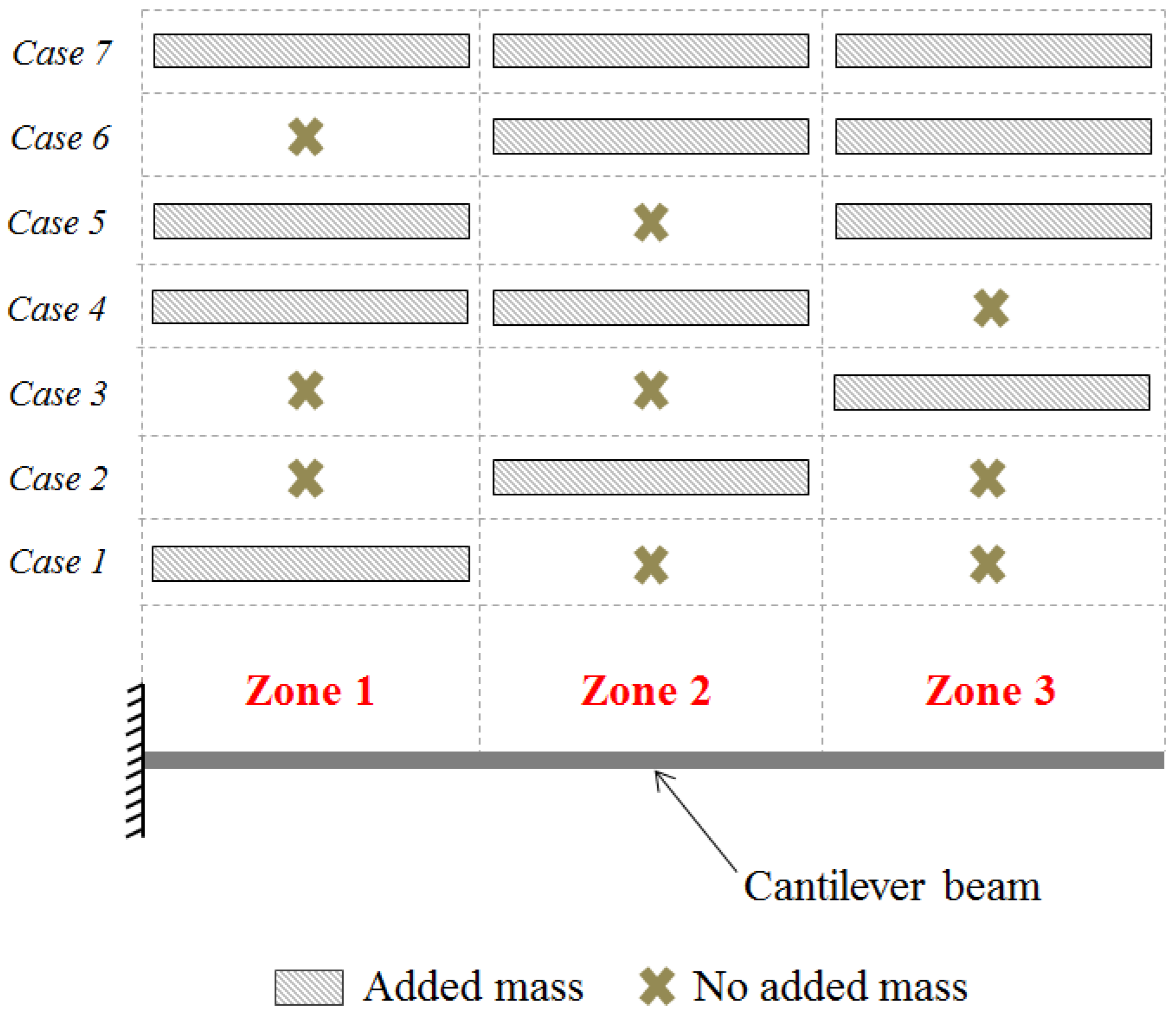
In the current work, ANN is used for function mapping between natural frequencies of the beam and added masses (which have two features: the location and the quantity of mass). For this, the beam is divided into three zones, and different added masses are considered with constant linear mass densities (mass per unit length) in these zones, as shown in Figure 7. Natural frequencies of the beam are calculated from the eigenvalue analysis of the EOM with added masses. The set of beam natural frequencies and corresponding added masses in the three zones are considered as one sample in the dataset. The natural frequencies calculated from the eigenvalue analysis of the EOM by considering 27 g of added mass on the beam in only one zone at a time are shown in

Table 4. Natural frequencies of the beam calculated with added mass of 27 g.

Vibration Mode	Natural Frequency (Hz)
	Added Mass 27 g in Zone 1	Added Mass 27 g in Zone 2	Added Mass 27 g in Zone 3
1st Bending	20.24	19.86	18.58
2nd Bending	123.64	118.00	122.52
3rd Bending	333.85	340.73	337.96

, where each frequency reduces differently with the location of added mass. This particular value of mass is chosen because later in this work, a mass equal to this value was considered on the experimental setup shown in Figure 1 and its natural frequencies estimated.

As discussed before, the network parameters need to be found by the trial and error method, which makes the process of finding network parameters cumbersome. However, based on the training data and the problem under consideration, these parameters can be chosen, which is outlined as follows.

• Number of outputs ($n_{o/p}$): This value is fixed at three in the current problem, which are the added masses in the three zones divided on the blade, as shown in Figure 7. Increasing this number makes the function approximation problem more complex, which requires more natural frequencies as input to find a valid relation between the inputs and outputs of the network.
• Number of inputs ($n_{i/p}$): For the current problem, natural frequencies of the beam are used as an input to the network. We can choose any number of natural frequencies of the beam as inputs; however, it would be advantageous if the added mass is detected with the minimum number of frequencies. The minimum number of frequencies required to detect added masses in the three zones is found in this study as three. It is not able to fit a valid model when the lower number of frequencies is used as an input to the network. Thus, first three natural frequencies of the beam are used as an input to the neural network.
• Number of hidden layers: Neural networks with one hidden layer and the sigmoid function as an activation function can approximate continuous functions with arbitrary precision [15]. Therefore, only one hidden layer is chosen in this study.
• Number of neurons ($n_{neu}$): When neural networks are used for classification tasks with d-dimensional input data, neurons in the hidden layer function as hyperplanes that partition d-dimensional space into various regions. For classifying d-dimensional input data into M clusters using the single-layer network, the number of hidden layer neurons required is M [15]. If two classes are defined for the added mass like light and heavy with respect to the mass of the beam in each zone, then eight classes of combinations of added masses are possible in three zones. If three classes are defined for the added masses like light, moderate and heavy in each zone, then 27 classes of added masses are possible in three zones. Therefore, eight and 27 neurons are considered in the hidden layer.
• Number of samples in the dataset used for training ($n_{sample}$): A rule of thumb, obtained from related statistical problems, is to have at least five- to ten-times as many training samples as the number of weights and bias variables used in the network to be trained [15]. From the above discussion, the number of inputs, the number of outputs and the number of hidden layers are fixed. The number of neurons is only varied; accordingly, the number of weights and bias variables used in the network will change. If $n_{neu}$ number of neurons is considered in the hidden layer, then the number of weights and bias variables to be determined in the network training is given by $n_{variables}=(n_{i/p}+1)n_{neu}+n_{o/p}(n_{neu}+1)$. In this study, the number of samples considered in the training data is such that they are greater than five- and ten-times the number of variables to be determined in the network. Each sample in the dataset consists of $n_{i/p}$ inputs and $n_{o/p}$ outputs.

The training dataset should cover possible added mass values and their combinations in the three zones for a better prediction of these added masses. In this study, 30% of the beam mass is considered as the maximum possible added mass, which is further split into three parts for the three zones. Therefore, a maximum of 10% of the beam mass is considered as a possible added mass in each zone while generating the training dataset. The two possibilities of no added mass and some mass value m in each zone in Figure 7 generated seven possible combinations of added masses in three zones. If n added mass values are considered in the range of 0%–10% of beam mass in each zone, then $(n^3-1)$ combinations of added masses are possible in the three zones. The smallest value of n is chosen in such a way that it satisfies the criteria for the number of samples required in the dataset (i.e., greater than five- and ten-times the number of variables to be determined in the network).

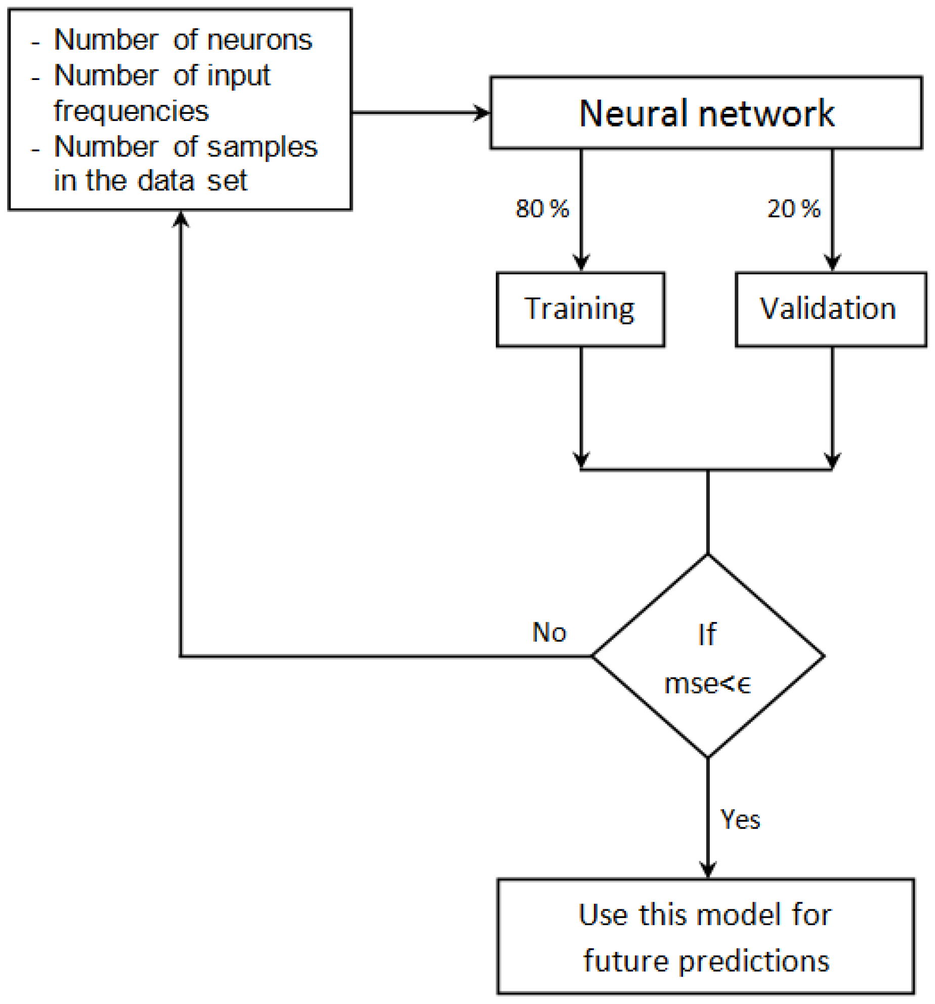
Four neural network models considering different network parameters given in

Table 5. Neural network model parameters.

Network Parameters	${\mathit{n}}_{\mathit{sample}}\ge 5\left({\mathit{n}}_{\mathit{variables}}\right)$		${\mathit{n}}_{\mathit{sample}}\ge 10\left({\mathit{n}}_{\mathit{variables}}\right)$
	Model 1	Model 2	Model 3	Model 4
Number of inputs ($n_{i/p}$)	3	3	3	3
Number of outputs ($n_{o/p}$)	3	3	3	3
Number of hidden layers	1	1	1	1
Number of neurons ($n_{neu}$)	8	27	8	27
Number of samples	342	999	728	2196
in the dataset ($n_{sample}$)

are designed using the MATLAB Neural Network Toolbox [22]. The design process is outlined in the flowchart shown in Figure 8. While designing the network, the dataset given as an input to the network is divided into two sets: 80% for training and 20% for validating the neural network model. The training set is used for computing the gradient (rate of change in $mse$ with the variation of weights and biases used in the network) and updating the network weights and biases. The error on the validation set is monitored during the training process. The validation error normally decreases during the initial phase of training, as does the training set error. However, when the network begins to over-fit the data, the error on the validation set typically begins to rise. The network weights and biases are saved at the minimum of the validation set error. The mean square error ($mse$) between network output and actual output should be low for both sets of data (training and validation). In the current work, added mass is the output of the network, so the unit of $mse$ is kg${}^2$. A condition for $mse<ϵ$ with $ϵ=1\times {10}^{-10}$ is set for limiting the error below square of the 1% of the smallest added mass value used in the dataset. If the error is not acceptable, then the neural network is not able to fit a valid model for the dataset.

The neural network model designed using the MATLAB toolbox [22] with parameters corresponding to the Model 1 in Table 5 is shown in Figure 9. With the network parameters defined in Table 5, four different neural network models satisfying the condition for $mse<ϵ$ are designed. These network models are given natural frequencies estimated from experiments as inputs in the next section to identify added masses.

5. Results and Discussion

Experimental modal analysis is carried out on the cantilever beam setup shown in Figure 1 by placing different added masses in the three zones. These masses are attached to the beam using adhesive while performing the experimental modal analysis. Fourteen test cases of added masses are attached to the beam and estimated beam natural frequencies from the experimental modal analysis. The first seven test cases consist of two possibilities of no added mass or 11 g of mass in each zone, which generates seven possible combinations of added masses in three zones similar to those shown in Figure 7. The remaining seven test cases consist of two possibilities of no added mass or 27 g of mass in each zone. These added mass values are chosen such that they are less than the maximum added mass value (10% of the beam mass in each zone) used in the dataset to train the network in the last section. The natural frequencies estimated in the fourteen test cases are given as an input to the four neural network models designed in the last section to identify added masses. As the actual added mass values used in the experiment and the identified mass values in these cases are known, a metric called the weighted absolute percentage error ($WAPE$), as defined in Equation (4), is calculated for each test case. It is defined as the ratio of the sum of the absolute error in the identified masses in each zone to the sum of actual added masses used in that test case. This $WAPE$ is calculated for all fourteen test cases, and the mean value of these errors for the identified masses by four neural network models is compared in

Table 6. Mean of the error values calculated using Equation (4) for fourteen test cases. $WAPE$, weighted absolute percentage error.

Neural Network	Mean WAPE
Model 1	30.68%
Model 2	30.76%
Model 3	30.44%
Model 4	30.63%

. This metric indicates the overall error in the identified mass values in the fourteen test cases, and it does not change significantly for the four neural network models. That means, increasing the number of neurons and the number of samples in the dataset offers no improvement in the identified values when it is possible to design a neural network with the least number of neurons and samples in the dataset satisfying the condition for $mse$. 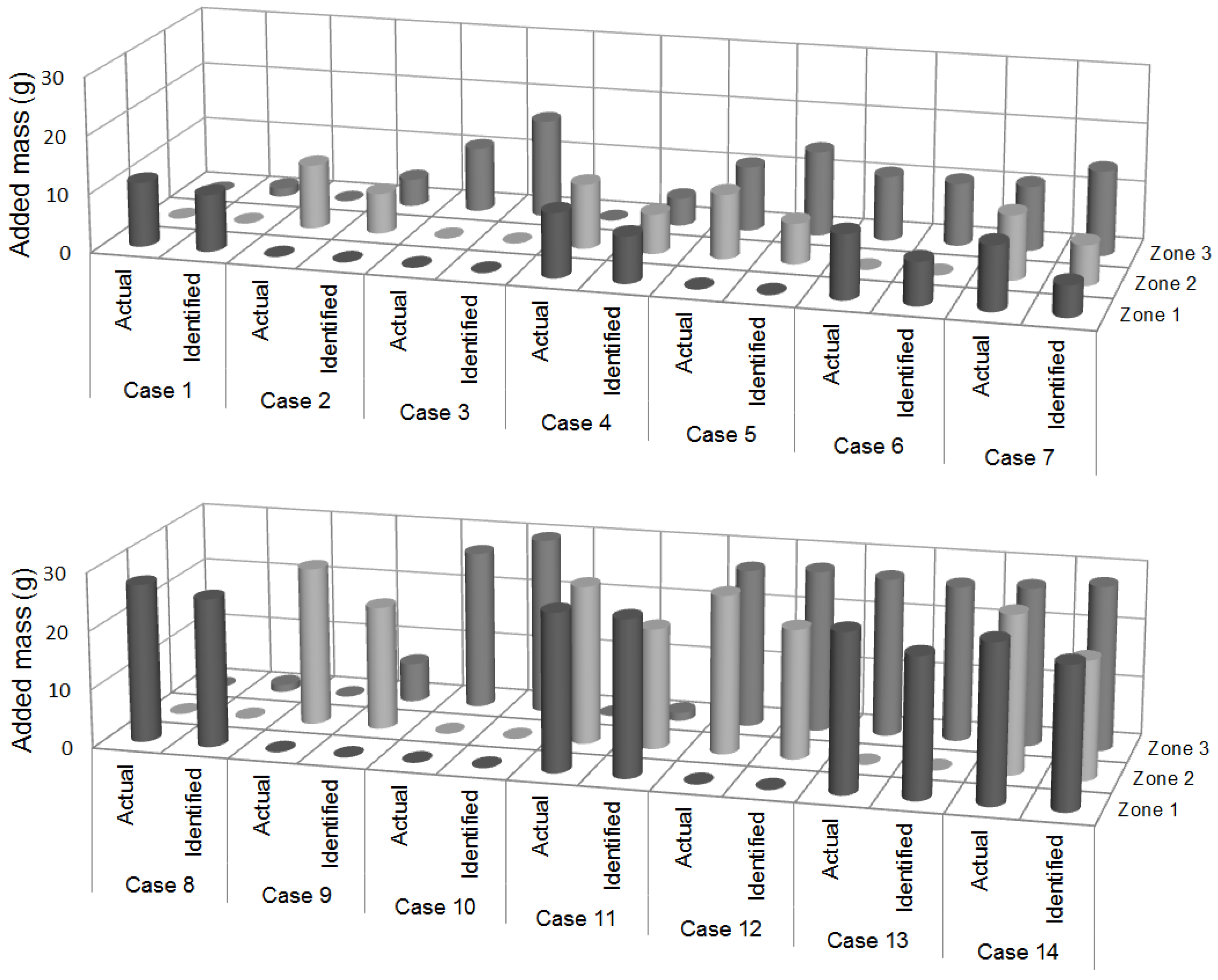The added masses identified in the fourteen test cases using the neural network Model 1 (refer to Table 5) are shown in Figure 10. 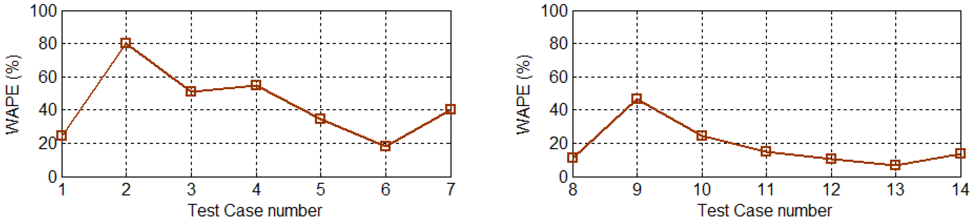The $WAPE$ calculated for the identified masses using the neural network Model 1 in each test case is shown in the Figure 11. This error changes with respect to the location and decreases with the increase in quantity of added mass.

$$WAP{E}_i=\frac{{\sum }_{k=1}^3\left|m_{actual}^{ik}-m_{identified}^{ik}\right|}{{\sum }_{k=1}^3{m}_{actual}^{ik}}$$

(4)

where i refers to the test case number; k refers to the zone number; $m_{actual}$, $m_{identified}$ refer to added masses actually used in the experiment and the value identified by neural network model, respectively.

The natural frequencies estimated from experimental modal analysis of the beam with added masses corresponding to the Test Cases 8–10 are given in

Table 7. Natural frequencies of the beam estimated from experimental modal analysis for the added mass Cases 8–10.

Vibration Mode	Natural Frequency (Hz)
	Added Mass 27 g in Zone 1	Added Mass 27 g in Zone 2	Added Mass 27 g in Zone 3
1st Bending	20.16	19.52	18.26
2nd Bending	123.59	118.90	122.97
3rd Bending	334.22	341.72	339.22

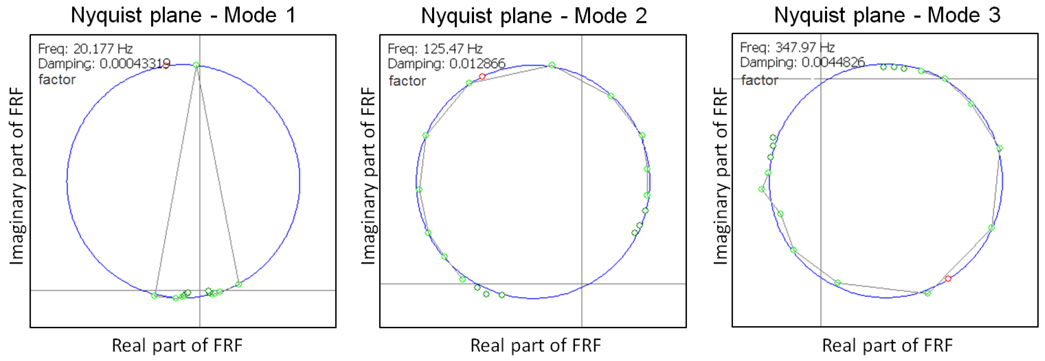
. It is clear from Table 4 and Table 7 that the natural frequencies calculated from the eigenvalue analysis of EOM and experimental modal analysis are not the same. While calculating the eigenvalues, added mass is modeled by increasing the mass density in the beam, whereas in the experiment, added mass introduces some damping due to the use of adhesive and also increases the stiffness of the beam locally. The damping factors in Test Case 14 (where 27 g is considered in all three zones) are identified using the circle fit method and shown in Figure 12. Damping in the structure is very low in both cases of no added mass and with added mass (refer to Figure 3 and Figure 12), which can be neglected (the assumption of no damping in the FEM model in Equation (2) is valid). It can be concluded that added mass in the case of experiments clearly increases the stiffness of the beam locally, due to which the natural frequencies increase. The reduction in frequency values with the increase in mass is higher than the increase in frequency values due to the local changes in stiffness, as a net effect, the natural frequencies estimated in the experimental added mass cases are higher than those calculated from the eigenvalue analysis. ANNs are generally used to predict the output of a function for a given input when it is trained with a dataset generated from a similar function. The network in the current case is trained with a dataset generated from a model where the influence of added mass is only considered on its mass properties, but it is tested with natural frequencies estimated from experiments where the added mass influences mass and structural properties of the beam, which means those frequencies correspond to a different function. In such cases, the neural network identifies added masses with an error. The proposed technique is only able to roughly estimate (with a mean $WAPE$ of 30.68% using the neural network Model 1) the added mass, and the error in identified masses is higher when the quantity of the added mass on the beam is smaller (refer to Test Cases 2 and 3 in Figure 11).

6. Application of the Proposed Technique to Wind Turbine Blade Ice Detection

The detection technique discussed in previous sections has the potential to be used for identifying ice mass accumulation on the wind turbine blades. There exist differences between the non-rotating cantilever beam structure used in the earlier sections and a rotating wind turbine blade. Therefore, the Tjaereborg 2 MW wind turbine blade is considered in this section to demonstrate the ice mass detection technique. Details about the structural and airfoil sections of the blade are reported in [23,24]. 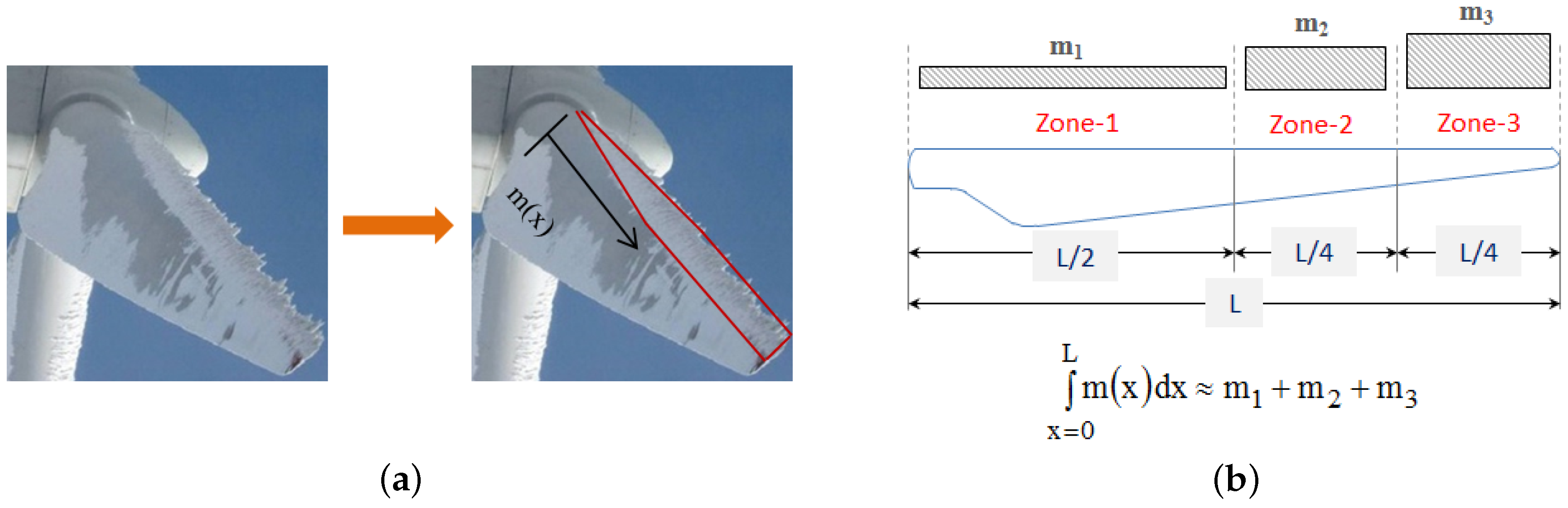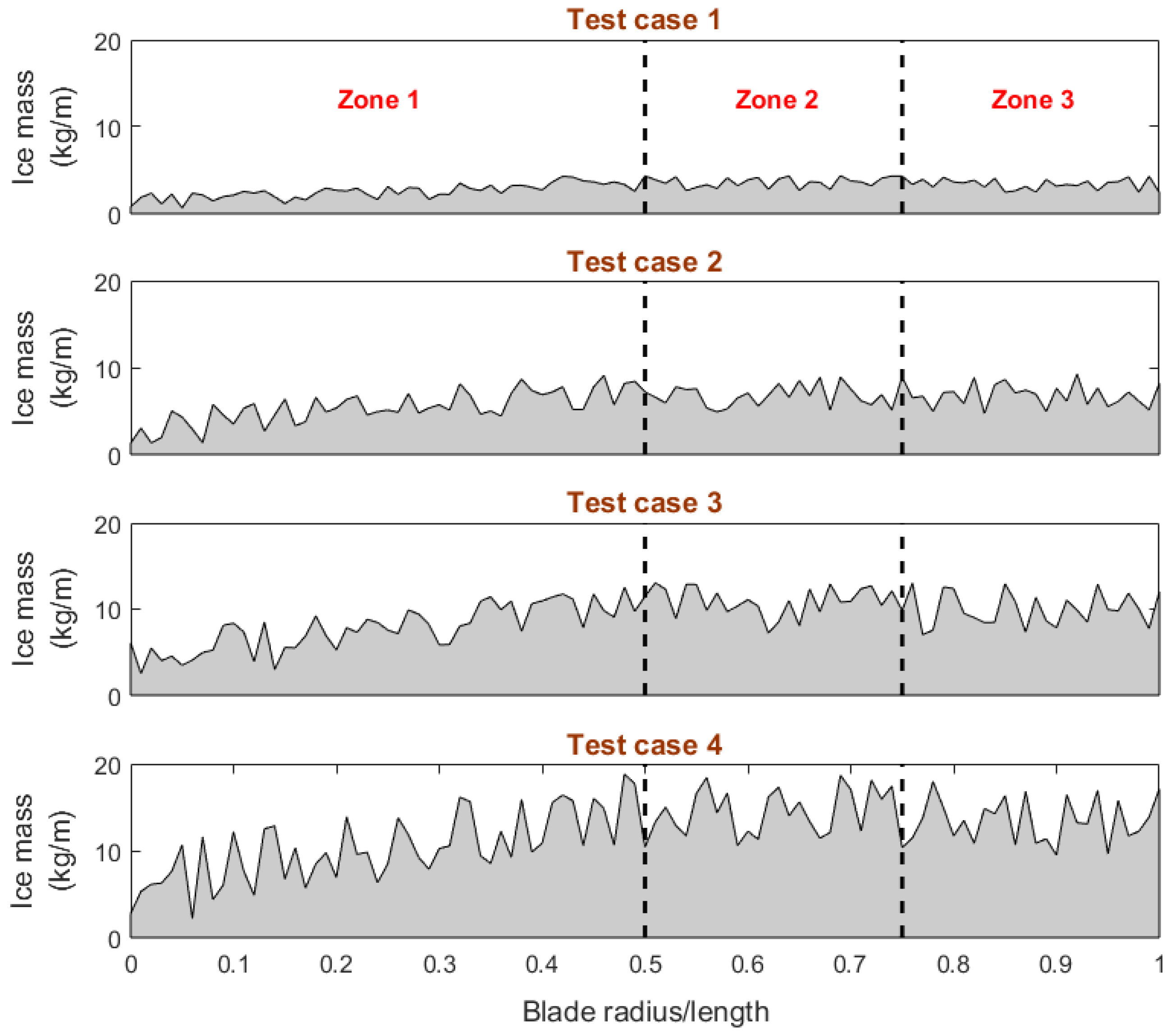In this section, the proposed technique is used to detect average ice mass accumulated on the blade (a typical mass distribution is shown in Figure 13a) by dividing its length into three zones, as shown in the Figure 13b. The inner half of the blade is considered as Zone 1, and the outer half of the blade is divided into two zones, Zones 2 and 3, which accumulate more ice than Zone 1. This is due to the fact that the airfoil sections in this part of the blade sweep more area in the rotation and also experience wind at higher relative velocity. The continuous ice mass distribution on the blade is reduced to three ice masses, which are distributed with a constant linear mass density, as shown in Figure 13b. This is the simplest approximation that is possible to represent a continuous ice mass distribution with minimum variables. This kind of approximation is also justified because de-icing systems of the blade are generally targeted to remove ice in specific locations. In such cases, the identification of ice mass in different zones makes it possible to remove ice effectively with minimum external power by activating the de-icing system in that part of the blade alone.

In the following subsections, the modal behavior of the current wind turbine blade is investigated to find natural frequencies of the blade that can be excited and also can be estimated from vibration measurements. Following that, a dataset of those frequencies is generated considering various masses in the three zones, and it is used to train a neural network model. Later, the trained network model is tested with the frequencies corresponding to four random ice mass distributions on the blade, and the identified ice masses are compared with the actual mass values used in those cases.

6.1. Modal Behavior of the Wind Turbine Blade

Aerodynamic loads generated by the wind blowing over the airfoil sections of the blade rotate the turbine, and dynamic changes in the wind and rotational motion induce vibrations in the turbine. The vibrations of the blade change the effective wind velocity, which influences the aerodynamic loads generated on the turbine. Thus, the structural and aerodynamic behaviors of the blades are coupled. 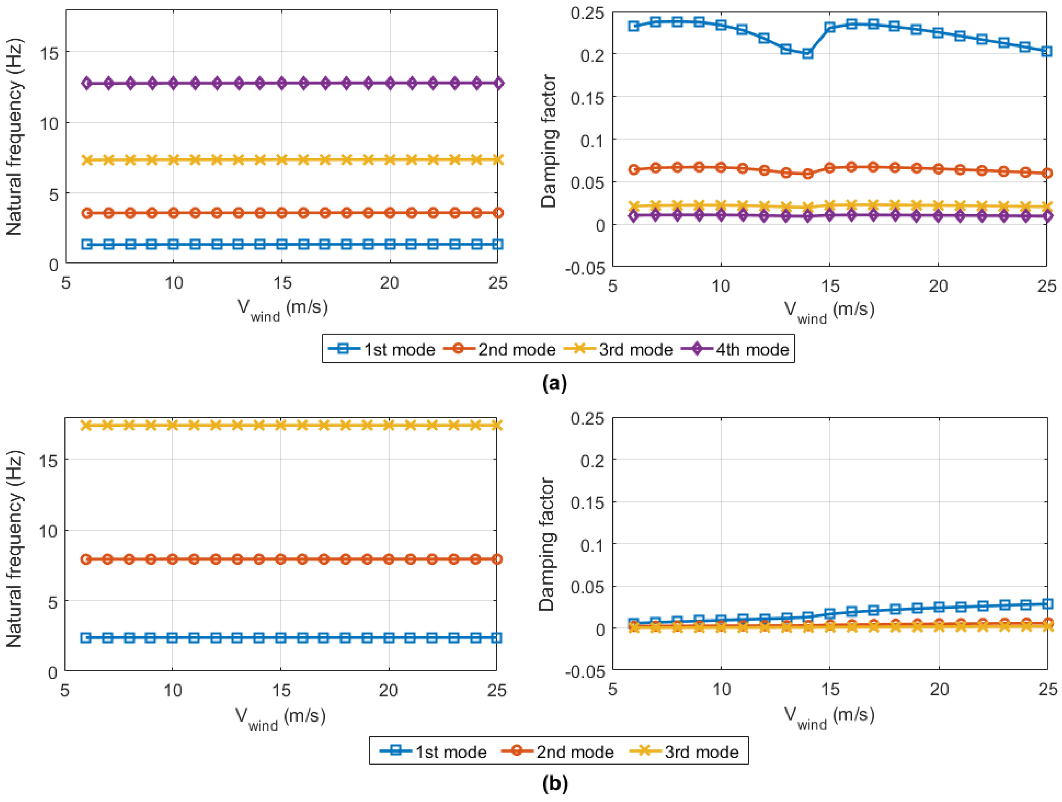Linear aeroelastic partial differential equations are derived in [7] considering this coupling between the structural and aerodynamic behavior of a wind turbine blade. Those equations are analyzed in this study using the finite element method (FEM) to calculate aeroelastic natural frequencies and damping factors of the current wind turbine blade, which are shown in Figure 14 over its operating wind speed range of 5–25 m/s. Aerodynamic loads modify the stiffness and damping in the aeroelastic equations of motion of the blade [7], and these loads vary with the wind speed, so the modal damping factors of the blade change accordingly. Natural frequencies slightly change with the wind velocities, and these changes are not noticeable in Figure 14, whereas the modal damping changes are noticeable. It can be observed that the flapwise modes are highly damped compared to the edgewise modes, and especially, the first flapwise mode is the most damped mode; higher modes are comparatively less damped. Therefore, any external disturbance whose frequency is close to the first flapwise mode frequency will be dampened out quickly. The aeroelastic modal behavior of the blade is analyzed only to find out the low damped modes of the blade.

Due to the recent advancement in wireless sensor technology, it is now possible to measure blade vibrations while in operation. Turbulent wind blowing over the rotor area can be regarded as a random excitation to the wind turbine blade, which excites its natural frequencies. This is the working principle of ice detection systems like BLADEControl [11,12], fos4blade IceDetection [13] and Wolfel IDD.Blade [14]. These systems use an accelerometer installed on the blade to measure vibration accelerations, and ice is detected based on the deviations in blade natural frequencies from the vibration spectra [25]. 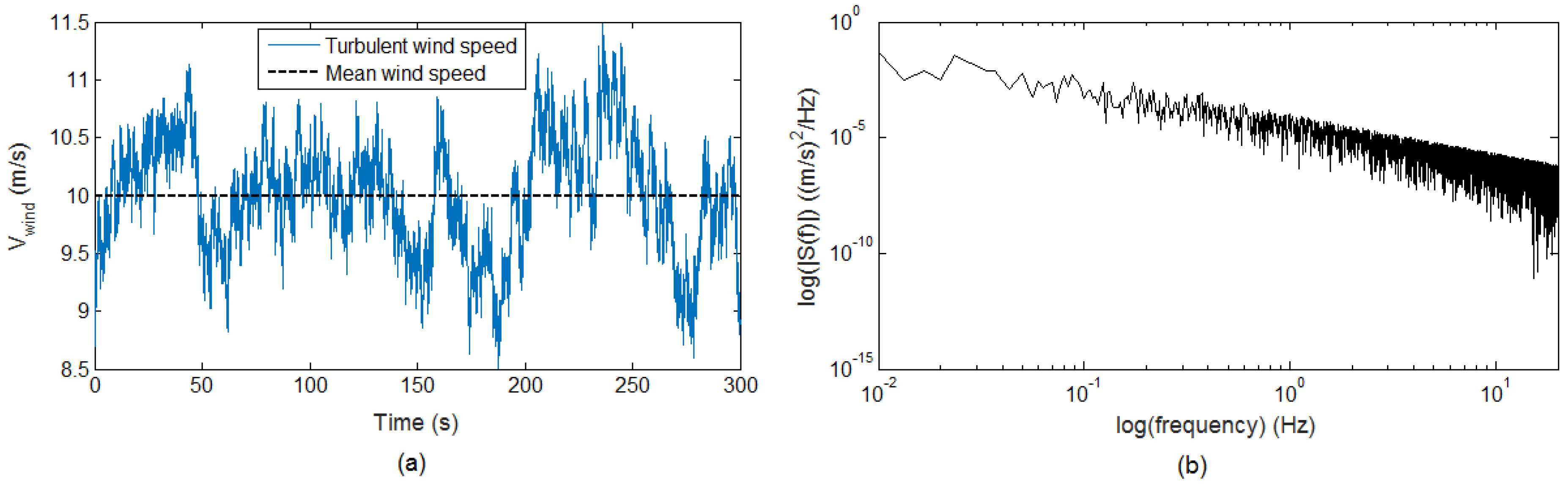These systems require a minimum wind speed of 2 m/s for ice detection [10]. A turbulent wind profile is generated using the QBlade software [26] over the rotor area of the current 2-MW wind turbine with a mean wind speed of 10 m/s at the nacelle height and a turbulence intensity of 5%. It is used to simulate the vibration response of the blade by solving differential equations obtained from the finite element solution of the aeroelastic equations derived in [7]. 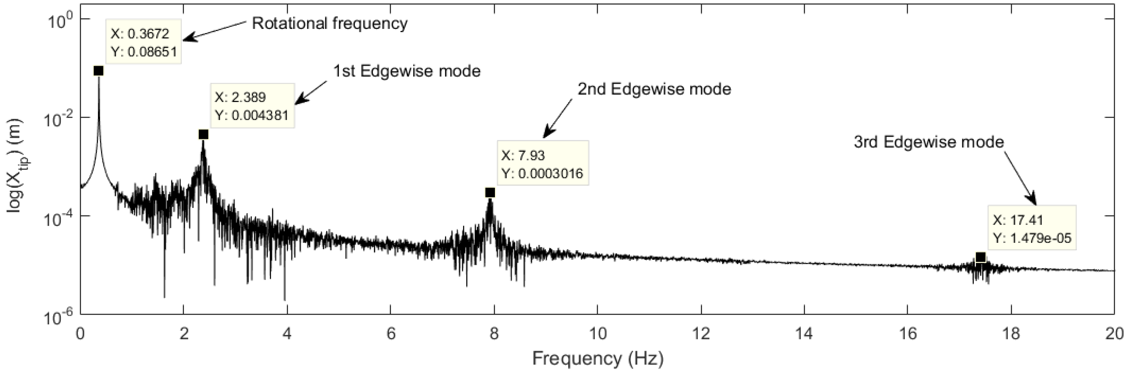The wind speed variation at nacelle height in the wind profile generated using QBlade software is shown in Figure 15a, and its power spectral density (PSD) is shown in Figure 15b. The power density of the turbulent wind speed is concentrated at low frequencies, and it decreases with increasing frequency, so the probability of exciting the first few vibration modes is higher. The Fourier transform of the blade’s edgewise vibration response at its tip location simulated using the turbulent wind profile is shown in Figure 16. The vibration response spectrum consists of a dominant frequency corresponding to the blade rotational frequency that is generally excited by the gravitational forces and wind shear, whereas the turbulence in wind excites the blade edgewise vibration modes. From Figure 14 and Figure 16, it is clear that the first few edgewise vibration modes can be excited by the turbulent wind due to their low damping, and also, these frequencies can be identified from the vibration measurements of the blade. This is the reason for the use of edgewise vibration spectrum analysis in the ice detection systems when the turbine is running and flapwise vibration spectrum analysis when the turbine is in the standstill condition [10]. The first three edgewise natural frequencies of the blade calculated from the eigenvalue analysis of the structural (the blade is assumed to be rotating in still air) and aeroelastic equations (evaluated at a wind velocity of 10 m/s) are compared with the frequencies estimated from the turbulent wind excitation response in

Table 8. Edgewise natural frequencies of the Tjaereborg 2-MW wind turbine blade.

Vibration Mode	Structural	Aeroelastic		Turbulent Wind Response
	Frequency (Hz)	Frequency (Hz)	Rel. Diff *	Frequency (Hz)	Rel. Diff *
1st Edgewise	2.392	2.381	−0.47%	2.389	−0.12%
2nd Edgewise	7.952	7.932	−0.25%	7.930	−0.28%
3rd Edgewise	17.424	17.414	−0.06%	17.410	−0.08%

* Relative difference in the frequencies is calculated with respect to the structural frequencies.

. The influence of aerodynamics on the edgewise natural frequencies is found to be marginal, and thus, it is neglected in this study. The dataset required to train the neural network is generated using the eigenvalue analysis of the structural equations of the blade. As the detection technique requires a minimum of three natural frequencies as an input to the network, first three edgewise natural frequencies of the blade are chosen as an input to the neural network.

6.2. Ice Accretion on the Blade

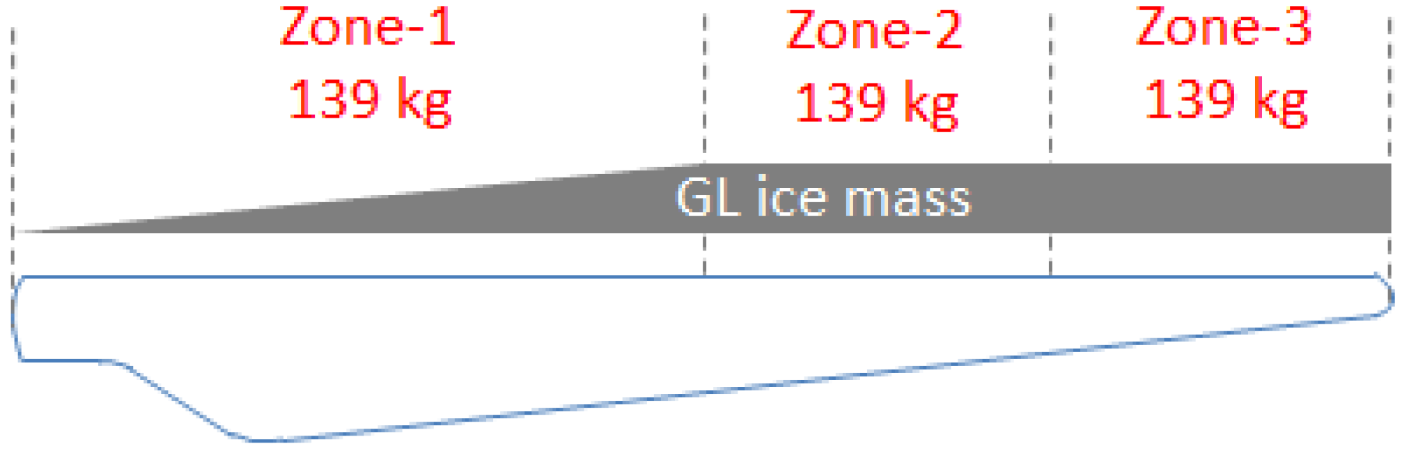
Ice formation on the blades depends on parameters like wind velocity, ambient temperature, liquid water content, median volume diameter or droplet size and the duration of the icing event. All of these parameters vary stochastically in space and time, and these parameters are different for different wind turbine sites and even change for turbines within the site. Ice accumulation on the wind turbine blades is not the same across the blade length. The blade accumulates more ice away from the root as it sweeps through a larger area in rotation and collects more ice. Ice on the blades causes more loads and vibrations in the turbine. In order to certify wind turbines and the components for the cold climate operation, Germanischer Lloyd (GL) [27] proposed a guideline that defines the maximum ice mass distribution on the blade to calculate loads acting on the turbine in various design load cases. The actual ice mass may be lower than this limit, but the turbines are certified for loads corresponding to this mass limit. Using this guideline, the maximum ice mass accumulation on this turbine blade is calculated to be 417 kg [7], which is distributed along the blade, as shown in the Figure 17. One third of this ice mass, i.e., 139 kg, is defined as the maximum ice mass that can be accumulated in each zone while generating the training dataset.

6.3. Artificial Neural Network Model

An artificial neural network model with network parameters $n_{i/p}=3$, $n_{o/p}=3$ and $n_{neu}=27$ is designed using the MATLAB neural network toolbox [22]. In this network, the number of variables to be determined in the training process is $n_{variables}=192$. In this study, the number of samples in the training data is chosen such that it is greater than five-times the number of variables to be determined in the network. A dataset consisting of 999 samples ($n_{sample}=n^3-1$) is generated by considering 10 different ice masses between zero and a maximum value of 139 kg (one third of the maximum ice mass limit defined by the GL specification) in each zone. These ice masses are distributed with constant linear mass density along the length of the zones, and blade natural frequencies are calculated from the eigenvalue analysis of the structural equations. Each sample in the dataset consists of three inputs (the first three edgewise natural frequencies of the blade) and three outputs (ice masses in the three zones). A condition for $mse<ϵ$ is set while designing the neural network model, where ϵ is defined as the square of the 1% of the smallest ice mass value used in the dataset. A neural network satisfying the condition for $mse$ is designed using the network parameters $n_{i/p}=3$, $n_{o/p}=3$, $n_{neu}=27$ and $n_{sample}=999$, and it is used to find average ice mass accumulated in the four test cases shown in Figure 18. The first three edgewise natural frequencies of the blade corresponding to these cases are given as an input to the trained neural network model, and the identified ice masses in these cases are compared with actual masses in

Table 9. Ice masses identified in the test cases.

Test Case No.	Location	Ice Mass (kg)		WAPE
		Actual	Identified
1	Zone 1	36	53	26.8%
	Zone 2	26	21
	Zone 3	25	26
2	Zone 1	75	72	2.2%
	Zone 2	51	49
	Zone 3	50	50
3	Zone 1	108	138	12.0%
	Zone 2	81	82
	Zone 3	74	74
4	Zone 1	143	179	12.4%
	Zone 2	108	102
	Zone 3	99	101

.

The ice mass in the four test cases is chosen in such a way that some part of it is distributed according to the GL specification (i.e., linearly increasing from root to half blade length and thereafter constant mass distribution), and the remaining part is distributed randomly along the blade length resembling the realistic ice mass distributions on the blade. The ice mass in these cases is distributed in a way different from the constant linear mass density distribution used to generate the training dataset. When the natural frequencies of the blade corresponding to these test cases are given as an input to the trained network, it will find equivalent cases of ice masses (distributed with constant linear mass densities) that will reduce the natural frequencies in a similar way. Ice mass in the Zone 1 is consistently over-predicted in the test cases. That means an ice mass distributed with constant linear mass density in Zone 1 reduces the natural frequencies in a similar way as the case of a comparatively lower ice mass whose mass distribution increases linearly along the length of Zone 1. The error in Zone 1 can be reduced by training the network with a dataset that considers an ice mass distribution similar to the GL specification. In reality, the nature of ice mass distribution differs from site to site based on the cloud heights, hub height, rotor diameter and operating conditions, so site-specific ice mass distributions can be captured using automatic cameras installed on the nacelle or spinner [10]. A training dataset with similar ice mass distributions can be generated to improve the accuracy of ice mass detection.

The technique proposed in this work requires first three edgewise natural frequencies of the blade as an input to the network for the ice mass detection. The natural frequencies of the wind turbine blade can be estimated from its vibration response due to ambient excitation (refer to Figure 16) or exciting the blade with some external excitation. The ambient excitation can only excite the first few natural frequencies of the blade, and it is also not certain if it can excite the frequencies required in the ice mass detection technique consistently all of the time. Ambient excitation has the drawback that it is not a controllable excitation that can be relied on. The detection technique becomes robust and reliable by using an external excitation system that can be controlled to excite blade natural frequencies. Lauristen et al. [28] proposed to use a pitch actuation system for blade excitation (different excitation signals like the frequency sweep of sinusoidal signals are possible) and to measure its vibration response using accelerometers installed at different locations on the blade. Ice can be detected based on the deviations in blade natural frequencies. The authors propose another idea to excite blade vibration modes using an eccentric rotating mass (ERM) driven by a DC motor. The unbalance force generated by the eccentric rotating mass varies with a frequency equal to the rotational frequency of the motor, which can be varied to excite the blade vibration modes with the corresponding forcing frequency. It is possible to excite higher modes of the blade. Spectrum analysis of the vibration response measured on the blade using an accelerometer enables one to estimate the natural frequencies of the blade. 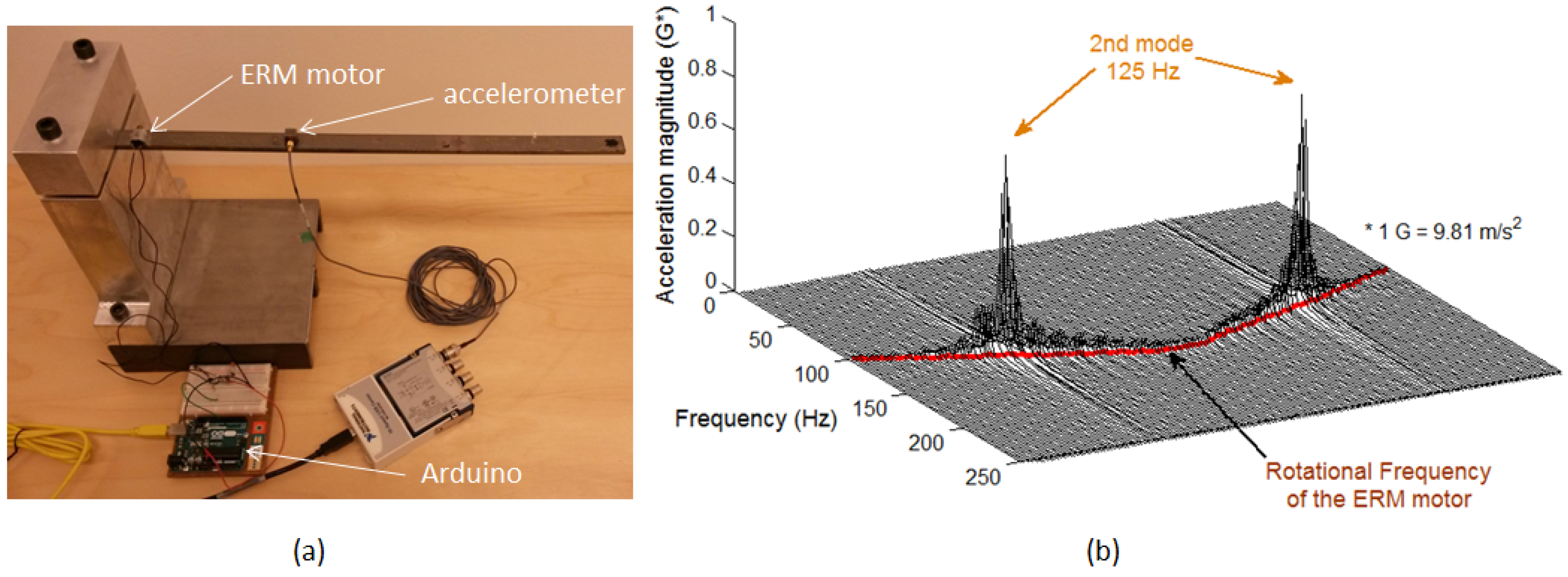This is just an idea similar to the electromechanical actuator proposed in [29] for the structural health monitoring of the blades and the dual de-icing system proposed in [30] that uses an ERM motor to excite low frequency vibrations. The proposed idea of the authors is evaluated on the cantilever beam experimental setup shown in Figure 19a, and a waterfall plot of the vibration response measured using accelerometer is shown in Figure 19b. In this experimental setup, the speed of the ERM motor is controlled using the pulse width modulation control in Arduino [31]. However, the feasibility of a similar system for exciting wind turbine blade vibration modes while it is rotating needs to be evaluated, and the authors are building a small scale-wind turbine experimental setup to evaluate this idea.

7. Summary and Conclusions

The natural frequencies of a structure reduce differently with the location and quantity of added mass. This behavior of the natural frequencies is used in the current study to train an artificial neural network model that identifies added masses for any given set of natural frequencies. The proposed technique is demonstrated on a non-rotating cantilever beam and a rotating wind turbine blade. The added masses in both cases are roughly estimated by the neural network model, and it requires a minimum of three natural frequencies as an input to the network to identify added masses in the three zones defined on their structures. A dataset of natural frequencies is generated considering different added masses at different locations on their structural models and used to train the network. The trained network model in the case of the cantilever beam is tested with the natural frequencies estimated from experiments considering different added masses on the beam. The added mass is modeled as an increase in the mass distribution of the structure while generating the training dataset. However, the added mass in the experimental setup introduces changes in the mass and stiffness properties of the structure. Due to this, the added mass values are identified with an error that changes with the location and quantity of added mass. The neural network (Model 1) identifies added masses in the fourteen test cases with a mean weighted absolute percentage error ($WAPE$) of 30.68%.

In the case of an application of this technique to wind turbine blade ice detection, natural frequencies required in the detection technique can be excited by the turbulent wind and estimated from the vibration measurements of the blade. The edgewise vibration modes of the blade are chosen as an input to the network, as these are the least damped modes that can be easily excited. The dataset required to train the network is generated using the finite element model of the blade considering different ice masses in the three zones defined on the blade. These ice masses are distributed with a constant linear mass density along the length of the zones. However, when the natural frequencies calculated using random mass distributions along the blade length in the four test cases are given as an input to the trained network model, it finds equivalent cases of ice masses (distributed with constant linear mass density), which will reduce the natural frequencies in a similar way as the frequencies corresponding to the test cases. Overall, the proposed technique predicts the ice mass distribution along the blade approximately. The error in identified masses varies with the nature of the ice mass distribution, and the maximum $WAPE$ occurs in Test Case 1, which is calculated as 26.8%.