Assessment of an Adaptive Load Forecasting Methodology in a Smart Grid Demonstration Project

Abstract

This paper presents the implementation of an adaptive load forecasting methodology in two different power networks from a smart grid demonstration project deployed in the region of Madrid, Spain. The paper contains an exhaustive comparative study of different short-term load forecast methodologies, addressing the methods and variables that are more relevant to be applied for the smart grid deployment. The evaluation followed in this paper suggests that the performance of the different methods depends on the conditions of the site in which the smart grid is implemented. It is shown that some non-linear methods, such as support vector machine with a radial basis function kernel and extremely randomized forest offer good performance using only 24 lagged load hourly values, which could be useful when the amount of data available is limited due to communication problems in the smart grid monitoring system. However, it has to be highlighted that, in general, the behavior of different short-term load forecast methodologies is not stable when they are applied to different power networks and that when there is a considerable variability throughout the whole testing period, some methods offer good performance in some situations, but they fail in others. In this paper, an adaptive load forecasting methodology is proposed to address this issue improving the forecasting performance through iterative optimization: in each specific situation, the best short-term load forecast methodology is chosen, resulting in minimum prediction errors.

1. Introduction

Load forecasting is a topic of great interest for electricity utilities because it enables them to make decisions on generation planning, the purchasing of electric power and future infrastructure development, and it is also very important for demand response actions. Load forecasting involves the accurate prediction of the electric demand in a geographical area within a planning horizon. Based on this horizon, load forecasting is usually classified into three categories [1]: Short-Term Load Forecasting (STLF) for a horizon within one day, Medium-Term Load Forecasting (MTLF) for one day to one year ahead and Long-Term Load Forecasting (LTLF) for one year to ten years ahead. This paper addresses an STLF scheme that will provide predictions from one hour to 24 hours-ahead where the variable to be forecasted is active energy consumption. The data used have been gathered from the OSIRIS (Optimisation of Intelligent Monitoring of the Distribution Network) project: an experimental implementation of a smart grid demonstration project in the Madrid area managed by the Utility Gas Natural Fenosa. In this area, there are different types of networks (residential, commercial and industrial).

In their most general form, short-term load forecasting models can be classified into two broad categories: statistical approaches and Artificial Intelligence-based (AI-based) models. Both models forecast the load demand based on historical data and/or exogenous variables, such as weather, day of the week, day of the year, type of day (e.g., holidays) and demand profiles. There are several statistical approaches that have been widely used in load forecasting problems in the past [2]. Similar-day methods are the most straightforward procedure and are based on searching for days in the historical data that share some common characteristics (such as day of the week, day of the year, type of day and weather) with the forecasted day. Regression techniques express the power demand as a linear function of one or more explanatory variables and an error term. Exponential smoothing, a variation of linear regression, gives an accurate and robust prediction that is inferred from an exponentially-weighted average of past observations [3]. Holt–Winter’s method [4] is a relevant example of exponential smoothing techniques. Load forecasting techniques based on stochastic time series assume, in their simplest form, that the future load demand is only a function of the previous loads. The input of the algorithm is the load demand pattern of historical data [5]. The most common techniques in this field are known as Auto-Regressive models (AR), which require making the assumption that the load can be defined as a linear combination of previous loads, and Moving Average (MA), which fits a linear regression between the white noise error terms of the time series. Both techniques can be combined (i.e., ARMA) and expanded to non-stationary processes by using the integrated moving average (i.e., ARIMA). If the load is dependent on external variables, such as sociological variables, variations of the previous techniques may be applied (i.e., ARMAX). In [6], univariate models for STLF based on linear regression and patterns are used, reducing the number of predictor to a few.

Lately, load-forecasting techniques have focused on non-linear methods. These methods usually depart from classical statistical approaches and bring in techniques from other fields of knowledge, such as machine learning or pattern recognition. Compared to classical statistical methods, artificial intelligence-based methods are more flexible and can cope with higher degrees of complexity. Several Artificial Intelligence (AI) methods have been proposed for STLF, such as Artificial Neural Networks (ANNs) [7,8,9]. Other techniques include fuzzy logic [10] and expert systems [11]. In [12], a novel methodology based in random forest is used to improve feature selection and enhance prediction accuracy. Support Vector Regression (SVR) has been proposed as a feasible alternative to ANNs. Support Vector Machines (SVM) have been used to win the EUNITE (European Network on Intelligent Technologies for Smart Adaptive Systems) competition, as explained in [13]. In [14], the least-square version of SVM regression is used to forecast daily peak load demand. Hybrid load forecasting frameworks have been used lately, which combine both statistical approaches and artificial intelligence-based models [15]. In [16], a meta-learning system is proposed, which automatically selects the best load forecasting algorithm out of seven well-known options based on the similarity of the new samples with previously analyzed ones, considering not only univariate data, but also multivariate data. As an improvement to traditional forecasting algorithms, other novel hybridizations have been proposed lately, such as chaotic evolutionary algorithms hybridized with SVR [17] or least squares SVM with fuzzy time series and the global harmony search algorithm [18].

In this paper, an exhaustive comparative study is presented comparing several methods applied to a short-term load forecasting in two smart grids’ deployment. Moreover, a novel adaptive load forecasting methodology is proposed that offers the capability to dynamically adapt its performance to the different situations of the power grid and even to different power networks (i.e., different types of clients, different aggregation level and different number of customers). This methodology is able to provide the best STLF method, which fits better to each specific situation. To the best of the authors’ knowledge, this procedure has not been considered in the existing literature, thus representing one of the main contributions of the paper.

This paper is structured as follows. In Section 2, an overview of the project from which the data have been obtained is presented. A description of the forecasting methods used and the evaluation methodology are explained in Section 3. In Section 4, the experimental results for the different forecast methods are presented. The adaptive load forecasting methodology is presented in Section 5. Results are based on a large collection of data, obtained from real electrical networks. The conclusions drawn from these results are discussed in Section 6.

2. Description of the Demonstration Project

The data used in this evaluation correspond to the smart meters’ measurements deployed at the OSIRIS project. The OSIRIS project is an innovation project to develop knowledge, tools and new equipment, to optimize the supervision of the smart grid that the Utility Gas Natural Fenosa is deploying in the Spanish national smart meter roll out. The project scenario is a primary substation which provides 240-MW of power to a region located in the south of Madrid (Spain), with 24 medium voltage feeders, 167 secondary substations and 25,849 customers. The distribution power network of the OSIRIS pilot is heterogeneous and involves different Low Voltage (LV) networks (rural, urban and semi-rural). The main objectives of the project are to implement an advanced distribution automation system, active remote metering and active energy management functionalities, to develop an optimum and interoperable smart grid architecture.

In this paper, the main findings obtained when STLF was applied in several LV networks of the OSIRIS project are detailed.

2.1. Overview of the Deployed Communications Infrastructure

The performance of any forecasting methodology relies heavily on the available data, notably on the number of data and the quality of the measurements. For this reason, ICT (Information and Communications Technologies) play a key role in smart grids because they are crucial to both enable the required almost real-time bidirectional information exchange and make the appropriate decisions based on the huge amount of gathered data at the required time. Although this paper is focused on the second part of the former sentence, it is worthwhile addressing the M2M (Machine-to-Machine) communications network that allows collecting part of the data used in the assessed STLF methods (notably, the historical hourly measurements), as well as enforcing the potential decisions made based on such STLF methods by carrying the resulting commands all the way down to the consumption points (e.g., if demand response programs were operated).

Communications networks for smart grids need to meet specific requirements from both technical and economic perspectives, such as low latency, high reliability, high levels of security and privacy or minimum deployment and operational costs [19,20,21]. Therefore, much research has recently been carried out on what the most appropriate communications architectures and technologies for smart grids are, based on simulations and actual deployments [22,23]. However, there is not a single answer to this question, since this depends on multiple factors, such as the target application [24], the specific features and constraints of the underlying power infrastructure or the specific regulation of each country.

As a result, there is a plethora of communications architectures and technologies available within the scope of M2M communications for smart grids [25,26], ranging from monolithic architectures based on a single communications technology (e.g., cellular) to hierarchical and heterogeneous architectures that involve different communications technologies depending on the specific requirements of each communications segment (the latter in general presenting higher flexibility and scalability than the former).

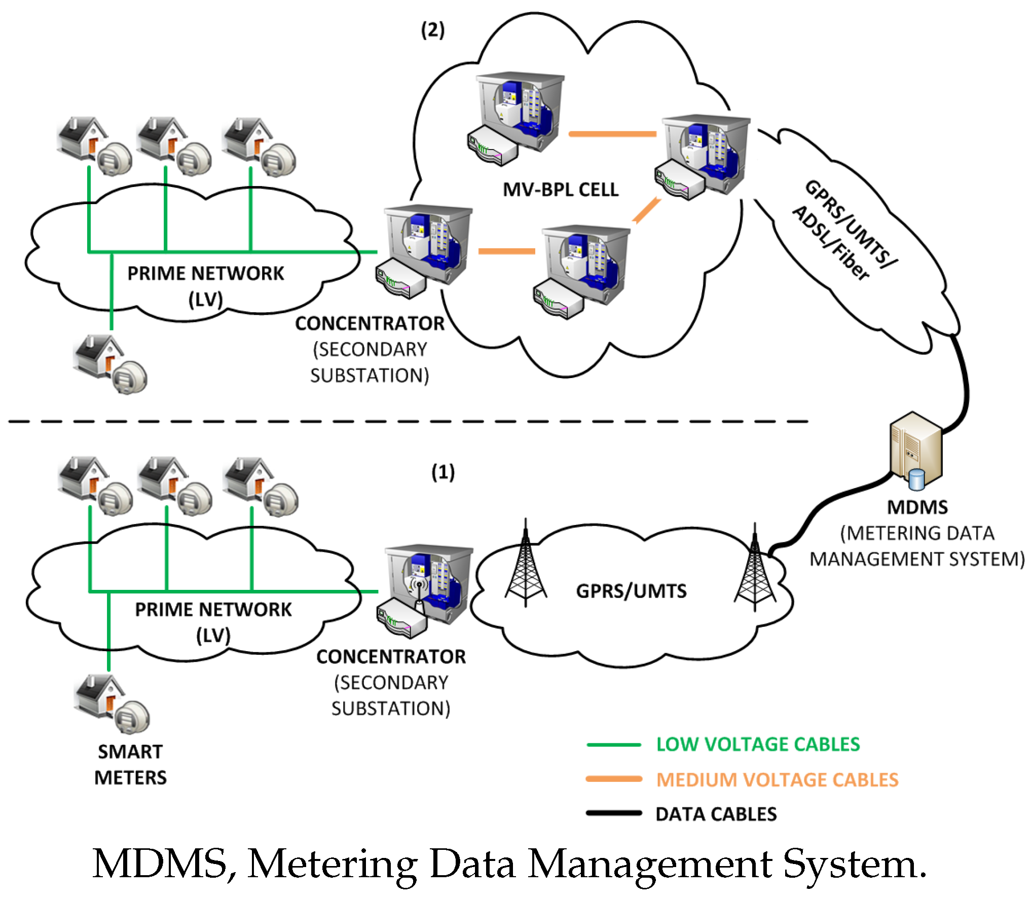
The communications infrastructure deployed in the pilot scheme of the OSIRIS project is explained in detail in [27]. Such a communications infrastructure is specifically designed to meet the boundary conditions of AMI (Advanced Metering Infrastructures) in Spain. Figure 1 shows an overview of the communications architecture and technologies. As can be seen, it is a hierarchical and heterogeneous communications network that involves two configurations, Configuration (1) being the most widely deployed in the field.

Both Configurations (1) and (2) used PRIME (Poweline Intelligent Metering Evolution) as the last mile communications technology. PRIME is a second-generation NB-PLC (Narrowband Power Line Communication) standard that uses the low voltage cable as a communications medium [28]. In Configuration (1), the communications between the concentrators of consumption data (located at the secondary substations) and the MDMS (Metering Data Management System), where operations like load forecasting are performed, are based on cellular technologies (typically, GPRS (General Packet Radio Service) or UMTS (Universal Mobile Telecommunications System)). In Configuration (2), however, concentrators organize themselves by setting up so called cells to send their data up to the so called gateway (which manages the communications with the MDMS), using the medium voltage infrastructure as a communications medium [29].

2.2. Data Analysis and Pre-Processing

The smart meter data of active energy readings of customers have been gathered by the supervisor meter of two of the seven networks operated by the OSIRIS project from November 2013–October 2015 (see

Table 1. Network characteristics.

Definition	Network 1	Network 2
Secondary substation rated power	400 kVA	630 kVA
Number of customers	63	433
Data collection period	2 years	2 years
Client type	Household	Commercial + household

). The supervisor’s meters are located in the low voltage side of the secondary MV (Medium Voltage)/LV substation and aggregate the measures of each group of customers connected to the secondary substation. Each customer has an individual smart meter that registers its individual hourly load demand. It has to be noted that the 1-h measurement resolution can be used by applications that need a very fast response, such as dynamic demand response. The first dataset (“Network 1”) contains 1-h kWh consumption data aggregated from 63 household customers. The second dataset used in this work (“Network 2”) contains 1-h kWh consumption data from an aggregated mixed group of 433 customers; including commercial and residential customers. In each case, the database is split into a training dataset, from November 2013–October 2014, and a testing dataset, from November 2014–October 2015.

Real implementations of smart meter deployments are subject to errors in measurements due to communication failures, corruption of the data or temporal unavailability of the meter. Those data are discarded from the dataset.

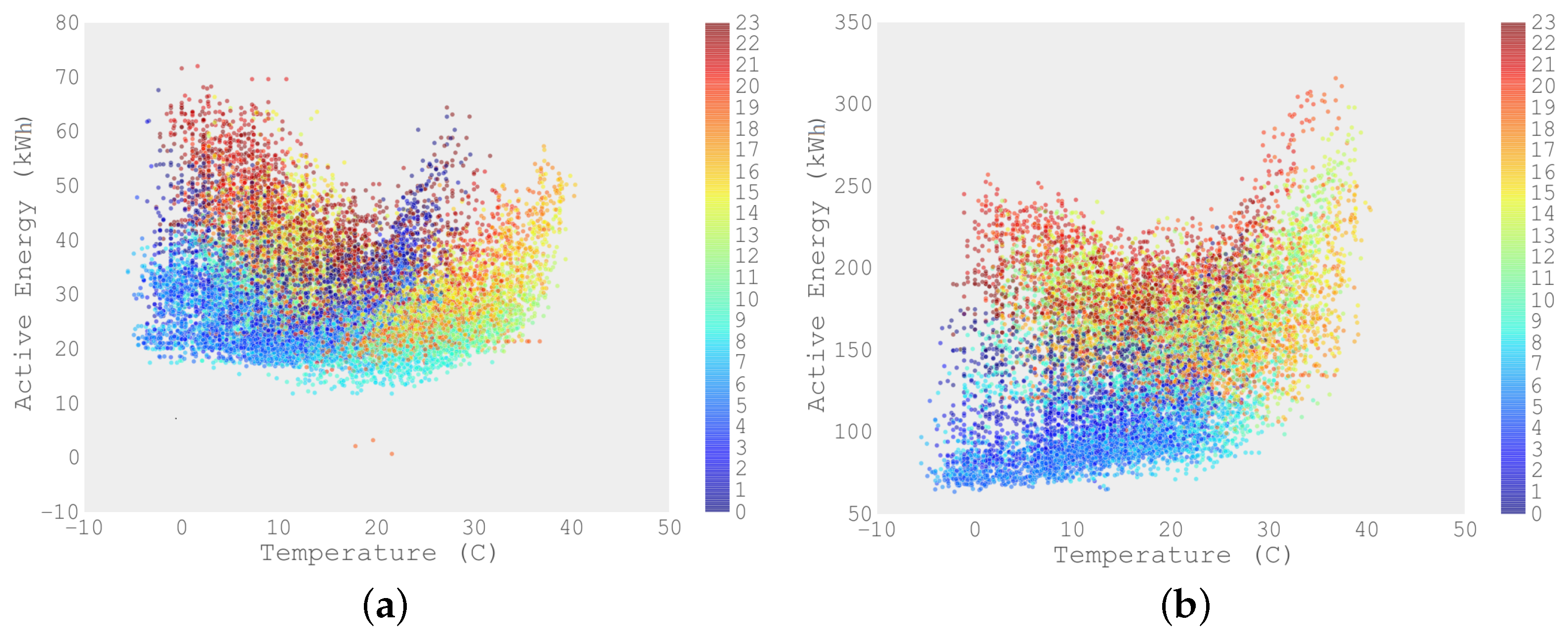
Figure 2 represents the correlation between the active energy, as captured in the low voltage side of the secondary substation of the MV/LV transformers (Network 1 and Network 2, respectively), and the temperature, as captured in its closest meteorological station in the Madrid area. The color-coded figure shows the dependence on the hour of the day. It can be noted that the active energy consumption has its highest value at approximately 10 p.m., especially during cold nights. It may be observed that in Network 1, the highest load values appear in the range of low temperatures; whereas in Network 2, the highest load values appear in the high range of temperatures. The difference could be due to the use of electrical heating equipment in Network 1 [30] and also because of the typical load profile in household customers in Spain, which corresponds to peak values at 19–22 h (evening) and at 11–14 h (morning). The load pattern of commercial customers is heavily influenced by opening and closing hours (9–21) and the use of cooling appliances during summer.

2.3. Analysis of Demand Correlations

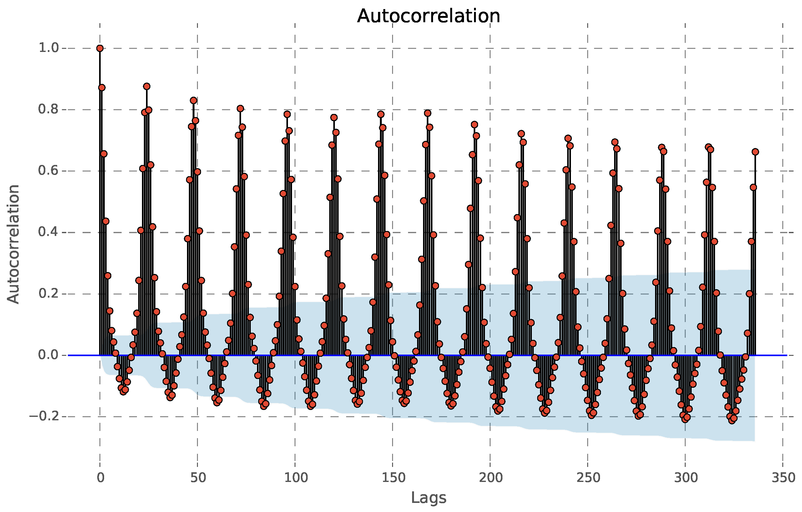
The active energy time series may be described as an autoregressive process, as derived by the application of the Box–Jenkins method [31] (Figure 3 and Figure 4). Figure 3 shows the correlation coefficients between the series and lags of itself over time. A distinctive pattern is observed, with periodical local maximums in the Autocorrelation Function (ACF), every 24 h. An additional weekly increase in the ACF can also be noticed. The autocorrelation declines in geometric progression from its highest value at Lag 1.

Load Baselines

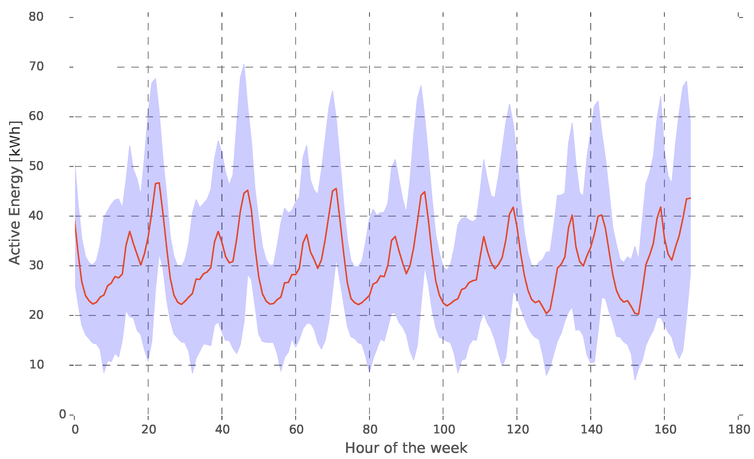
Regarding the load baselines, Figure 5 represents the average load grouped by hour of the week. The load pattern for each day of the week may be clearly seen in Network 1 (residential network). Working days follow a similar load curve; whereas weekends present two distinctive daily peaks: the morning peak results from the fact that more people have lunch at home on the weekends.

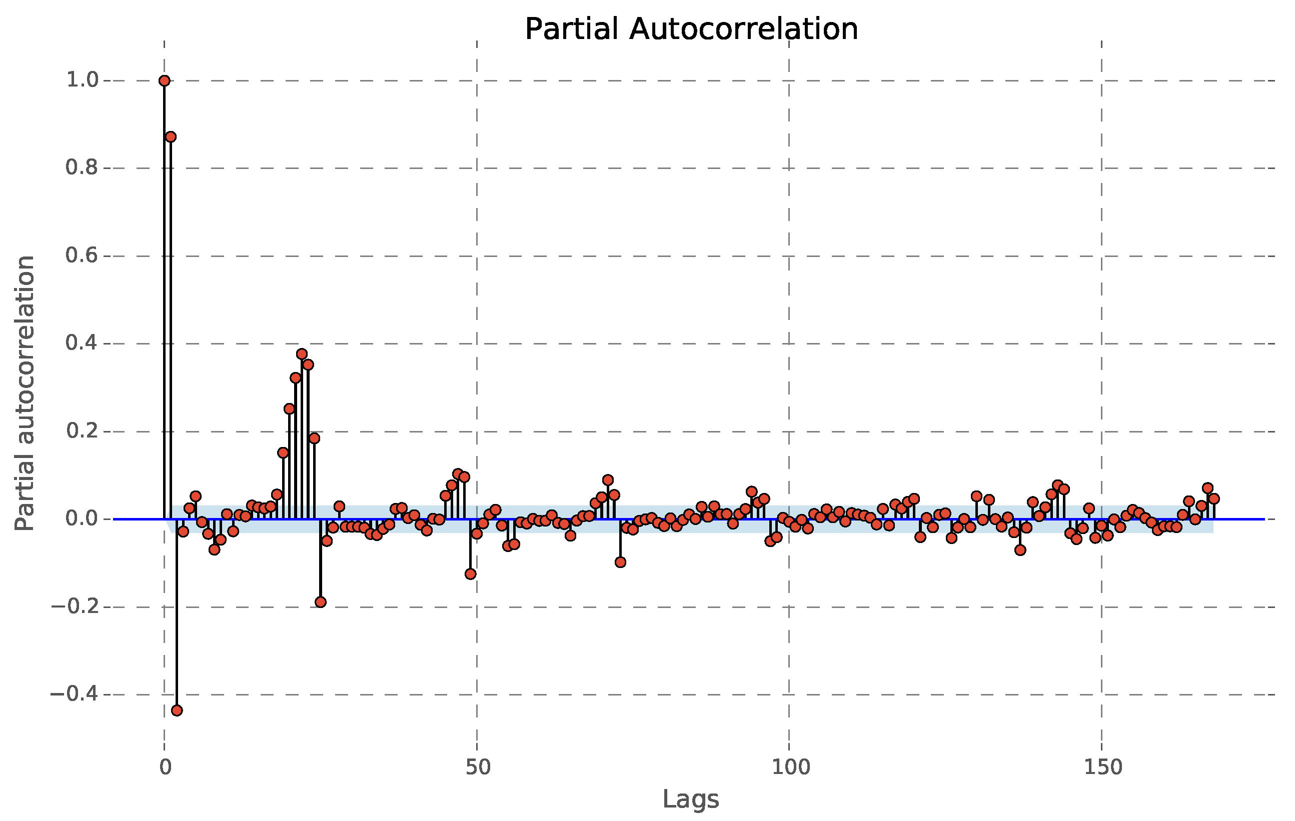
Figure 4 shows the Partial Autocorrelation Function (PACF) of the series. The PACF is cut off abruptly after Lag 1.

This suggests that the series does not have a significant Mean Average (MA) component; thus, the model does not contain lagged terms on the residuals.

3. Forecasting Methods and Evaluation Methodology

The methodology used to predict the future load demand is based on training linear models with an array of specially-designed features. The feature vector comprises:

• Lagged load measurements
• Calendar variables:

  –

  Time of day,

  –

  Day of the week (a number from 0–6 is assigned to every data point, allowing the model to differentiate workdays from weekends),

  –

  Day of the month,

  –

  Week of the year.

• Lagged temperature measurements
• Forecasted temperature measurements

3.1. Model

The power demand at time t is expressed as a non-parametric additive model:

$${\widehat{y}}_t=c(t)+l(y_t)+m(T_t)+{\epsilon }_t$$

(1)

where:

• ${\widehat{y}}_t$ is the predicted demand at time t.
• $c(t)$ is the contextual information at time t. This information contains calendar effects, such as the hour of the day and the day of the week.
• $l(y_t)$ is a series of recent demand measurements, going backwards from $t-1$.
• $m(T_t)$ models the forecasted meteorological conditions at time t, as well as recent measurements, going backwards from $t-1$.
• ${\epsilon }_t$ is the model error at time t.

3.1.1. Meteorological Information

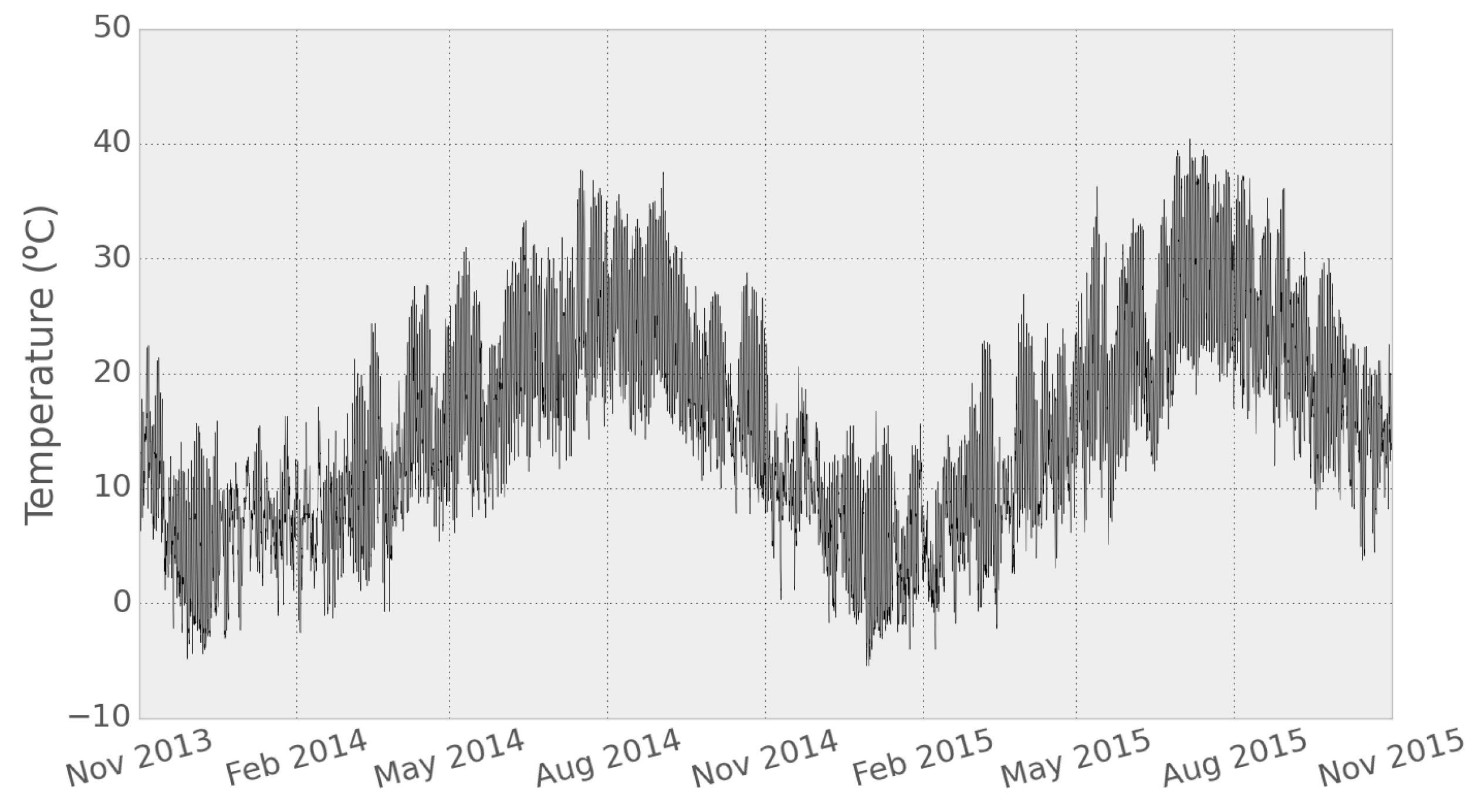
Meteorological factors are widely considered to have an influence on the power consumption, temperature being the one that influences the load demand greatly. The feature vector contains a varying number of lagged temperature measures, as well as the forecasted temperature collected from several weather stations in the Madrid area provided by AEMET (Agencia Estatal de Meteorologia) [32]. Lagged temperature values have been added for every load value used in the feature vector plus the forecasted temperature value for the forecasting hour. The meteorological section of the feature vector is $x_m(n)=\{T_1,\cdots ,T_n\}$. Figure 6 shows the hourly temperature values recorded at the nearest meteorological station of Network 1 during the data collection period.

3.1.2. Calendar Information

As shown in Figure 5, the load demand follows a distinctive pattern throughout the day and also within the same week. Two calendar features are included in the feature vector. The calendar section of the feature vector is $x_c=\{d,w\}$, where d is the hour of the day, encoded as a number between zero and 23, and w is the day of the week, encoded as a number between zero and six (zero for Mondays and six for Sundays).

3.1.3. Lagged Demand

Arguably, the most important regressor of a time series is its historical evolution in the past. The feature vector includes the lagged active energy, expressed in kWh, as $x_y(l)=\{y_1,\cdots ,y_l\}$, where $y_l$ is the load l steps in the past. Figure 3 shows that the lagged load measurements with the most significant correlation are $y_l=\{y_{12},y_{24},y_{48},y_{168},y_{336}\}$, corresponding to a half-day, one day, two days, one week and two weeks of lagged loads, respectively.

3.2. Methods

The linear auto-regressive models that have been fitted to the dataset, as well as the non-linear methods used to provide context are described as follows.

3.2.1. Linear Models

Assuming the future load can be expressed as a linear combination of the input values introduced in Section 3.1, the load forecaster can be expressed as:

$$\widehat{y}(w,x)=w_0+w_1{x}_1+...+w_p{x}_p$$

(2)

where $\widehat{y}$ is the predicted value, $X=(x_1,...,x_p)$ is the feature vector made from p inputs and $w=(w_1,...,w_p)$ are its coefficients.

• Ordinary Least Squares (OLS) methods fit a linear model with coefficients $w=(w_1,...,w_p)$ to minimize the residual sum of squares between the training set and the testing set samples, expressed via the equation:

  $$\underset{w}{min}{\left|\right|\widehat{y}(w,x)-y\left|\right|}^2$$

  (3)

  where $\widehat{y}(w,x)$ is the predicted value, as defined in Equation (2), and y is the real load value. The linear approximation is then used to predict future data.
• Bayesian Ridge regression (BR): Bayesian ridge regression is a variation of OLS and it imposes a penalty on the size of the linear coefficients. The ridge coefficients minimize a penalized residual sum of squares.

  $$\underset{w}{min}{\left|\right|\widehat{y}(w,x)-y\left|\right|}^2+\alpha {\left|\right|w\left|\right|}^2$$

  (4)

  where $\alpha \ge 0$ controls the penalization.
• Elastic Net (EN): This method fits a linear model regularized with $L_1$ and $L_2$. Elastic net is useful when there are multiple features that are correlated with one another. The study presented in this paper is such a case, where most of the input features are lagged loads. The elastic net linear forecaster minimizes the following cost function.

  $$\underset{w}{min}\frac{1}{2n}\left|\right|\widehat{y}(w,x)-{y\left|\right|}_2^2+{\alpha \rho \left|\right|w\left|\right|}_1+\frac{\alpha (1-\rho )}{2}{\left|\right|w\left|\right|}_2^2$$

  (5)

  where n is the number of samples, α is the factor that penalizes the coefficient size and ρ is the parameter that controls the combination between $L_1$ and $L_2$. The optimal values of α and ρ parameters are found by means of cross-validation on the training dataset.
• Support Vector Machines using a linear kernel (SVM-linear), introduced by Vladimir Vapnik [33], are a supervised learning method for solving classification and, later, regression problems. The original definition of SVM considered the separation of the feature space as a linear function.

3.2.2. Non-Linear Models

• Support Vector Machine using a Radial Basis Function kernel (SVM-RBF): The use of a RBF kernel allows the SVM algorithm to project the feature space into a higher dimensional space, allowing for non-linear mapping of the relations between the regressors and the target feature.
• Decision Tree (DT): DTs are a non-parametric supervised learning method used for classification and regression. The goal is to create a model that predicts the value of a target variable by learning simple decision rules inferred from the data features. The load curve is approximated with a set of if-then-else decision rules. Given a set of training vectors Q, the data are split into two sets, according to a threshold t of one of the features q. The split $\theta =(q,t)$ that better separates the data into two classes is selected. The algorithm is repeated on each of the branches until the maximum depth is reached.
• Random Forest (RF): This averaging method relies on the results of several decision trees, hence the name. Each of the trees is trained on a different subset of the training data with a replacement. As a result, the prediction of each one would be different. In this implementation, the forest is designed with 50 trees, as this has been found to be the optimum value via cross-validation on the training dataset. A variation of random forest is the Extremely Randomized Forest (ERF), which randomly selects the decision threshold of each tree.
• Gradient Tree Boosting (GB): GB is a generalization of boosting to arbitrary differentiable loss functions. This approach is robust to outliers and is able to handle mixed data types. In this implementation, binary decision trees are used. GB considers additive models. In each step of the algorithm, the new model $F_m$ is the addition of the previous model $F_{m-1}$ and the result of a minimization function. At each stage, the decision tree $h(x)$ is chosen to minimize the loss function L. Gradient boosting attempts to solve this minimization problem numerically via steepest descent.

  $$F_m(x)=F_{m-1}(x)+\arg \underset{h}{\min }\sum _{i=1}^{n}L(y_i,F_{m-1}(x_i)-h(x))$$

  (6)
• K Nearest Neighbors (KNN): A simple regression algorithm, nearest neighbors estimates the load, given a set of regressors, by averaging the numerical targets of the k closest neighbors learned from the training dataset. In this implementation, 10 neighbors have been used. The optimum number of neighbors has been found using cross-validation on the training dataset.

3.3. Evaluation Metric

There are different metrics to evaluate the performance of prediction models [34]. In this work, the forecasted load demand is evaluated by means of the Mean Absolute Error (MAE) and Mean Absolute Percentage Error (MAPE), as defined in Equations (7) and (8).

$$MAE(y,\widehat{y})=\frac{1}{n}\sum _{t=1}^n\left|y_t-{\widehat{y}}_t\right|$$

(7)

$$MAPE(y,\widehat{y})=\frac{100}{n}\sum _{t=1}^n\left|\frac{y_t-{\widehat{y}}_t}{y_t}\right|$$

(8)

where $y_t$ is the actual value, ${\widehat{y}}_t$ is the forecasted value and n is the number of samples.

Additional metrics, such as Root-Mean-Square Error (RMSE), are considered for the evaluation of the results, as defined in Equation (9).

$$RMSE(y,\widehat{y})=\sqrt{\frac{{\sum }_{t=1}^n{(y_t-{\widehat{y}}_t)}^2}{n}}$$

(9)

3.4. Parameter Cross-Validation

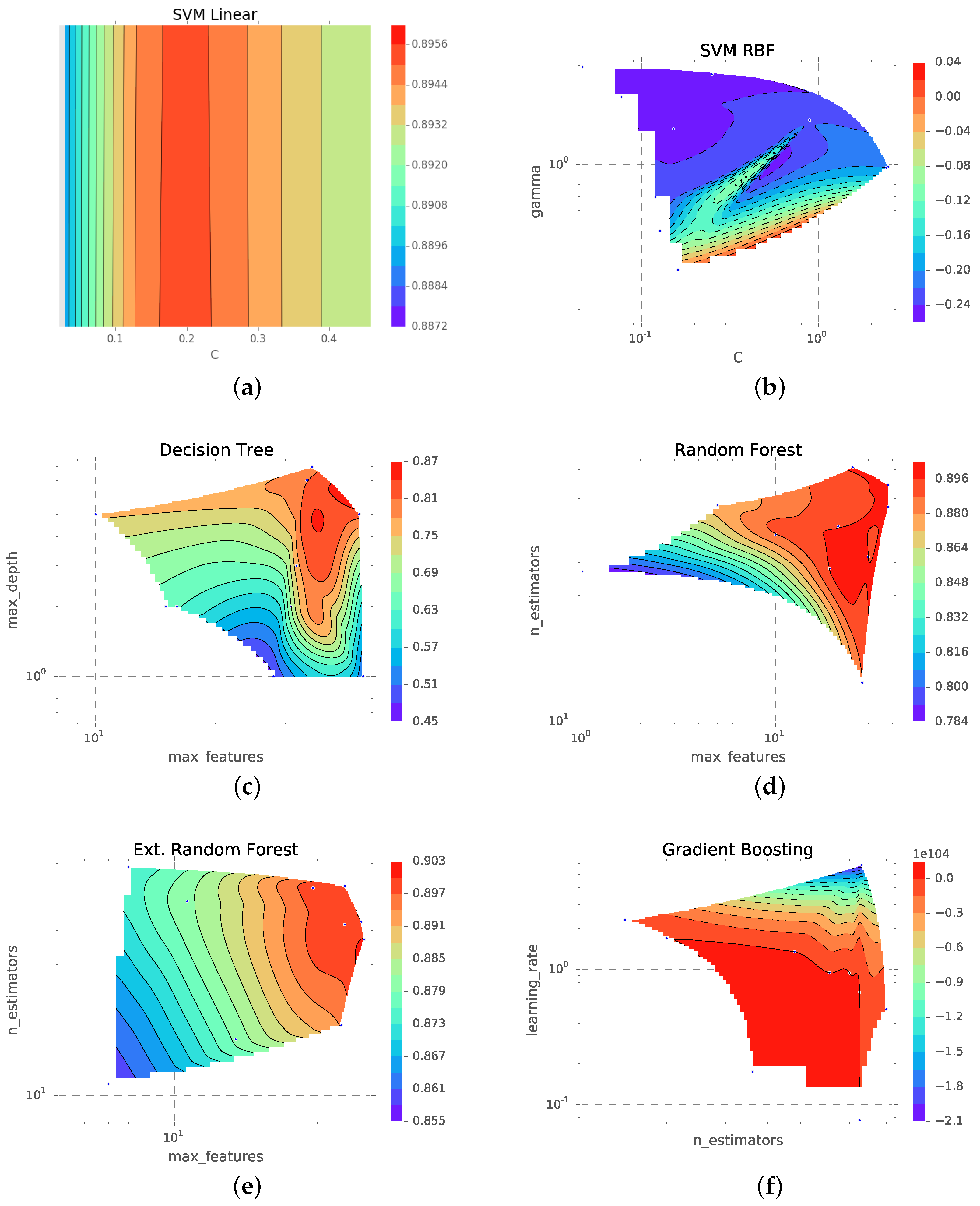
The most relevant parameters of each method are selected and set to a random value as part of the training procedure of each experiment. The score of those values is the three-fold cross-validation of the training dataset. This procedure is repeated for 20 points in the parameter hyperspace. The optimum point is found by minimizing the error in this space. Figure 7 shows a representative sample of six methods, where the parameter space is projected to the two most significant dimensions. By randomly sampling the parameter space, the optimum point is found. Figure 7a represents the parameter space projected to the soft margin parameter C. The SVM with an RBF kernel is projected in Figure 7b to C and γ, the radial basis function parameter. The most important parameters of the decision tree method are the maximum depth of the tree and the maximum number of features used (Figure 7c). Both approaches based on random forests (Figure 7d,e) are most dependent on the number of features used for each tree and the number of trees to aggregate. The most relevant parameter of the gradient boosting method is the learning rate, as the number of estimators is relatively unimportant. Other important parameters are α and ρ for the elastic net method, α for the Bayesian ridge regression and k for the KNN method.

4. Experimental Results in the Smart Grid Demonstration Project

Once the theoretical background is set and the different methods used for STLF have been introduced, the experimental results are presented in this section.

4.1. Feature Vector Design

The final feature vector is $x=x_y(l)\parallel x_c\parallel x_m(n)$, where || designates the concatenation operator. To evaluate the influence of each group of features, the evaluation assesses the impact of removing one or more of these groups from the feature vector. Likewise, the lag orders l and n are varied.

The feature vectors undergo a standardization process, where each individual feature is normalized so that the training subset is centered on zero and has unit variance. This pre-processing is needed for the SVMs and the regularizers of linear models. The testing dataset is then normalized by using the same parameters.

Number of Lagged Load Measurements

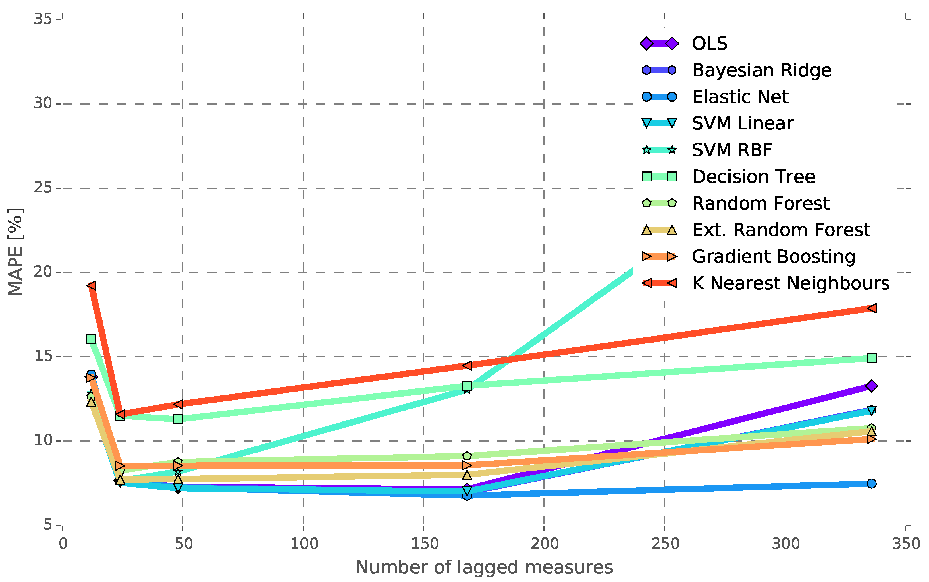
The most important features of the vector are the historical measurements of the load. As observed in Figure 3, the load has a repetitive pattern with two main frequencies, daily and weekly. Figure 8 shows the MAPE score of the different regression methods for an increasing number of lagged load measurements for power Network 1. Several numbers of lagged measures have been considered ($l=\{12,24,48,168,336\}$), and the lowest MAPE achieved depends on the used method. Linear models (OLS, BR, EN and SVM-linear) achieve their best performance for $l=168$ (one week) of lagged measures, although the difference of using $l=48$ is not significant (<1% MAPE). It may be observed that the elastic net method has a consistent performance for all of the numbers of lagged loads considered. The majority of the non-linear methods reaches their lowest MAPE for $l=24$, except DT, which performs better for $l=48$. Figure 8 also shows that the MAPE value of some non-linear methods (KNN, DT and SVM-RBF) quickly escalates for a number of lagged measures greater than 24. Both linear and non-linear methods (except KNN and DT, which show the highest MAPE values) have a similar performance when $l=24$.

4.2. Full Feature Vector

Table 2. MAPE score using all methods for the two smart grid power networks. BR, Bayesian Ridge regression.

Method	Network 1	Network 2
OLS	6012	3310
BR	5994	3305
EN	5381	3775
SVM-linear	7718	6972
SVM-RBF	6998	3685
DT	9415	5806
RF	6771	3426
ERF	6178	3162
GB	5822	3549
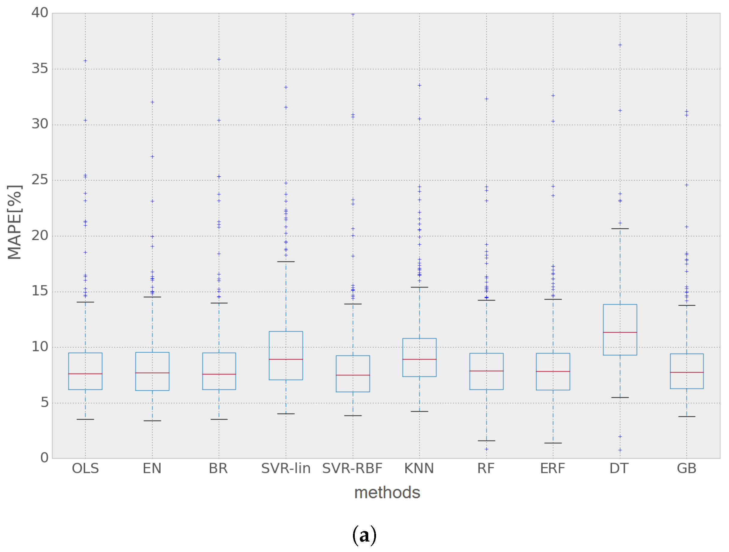
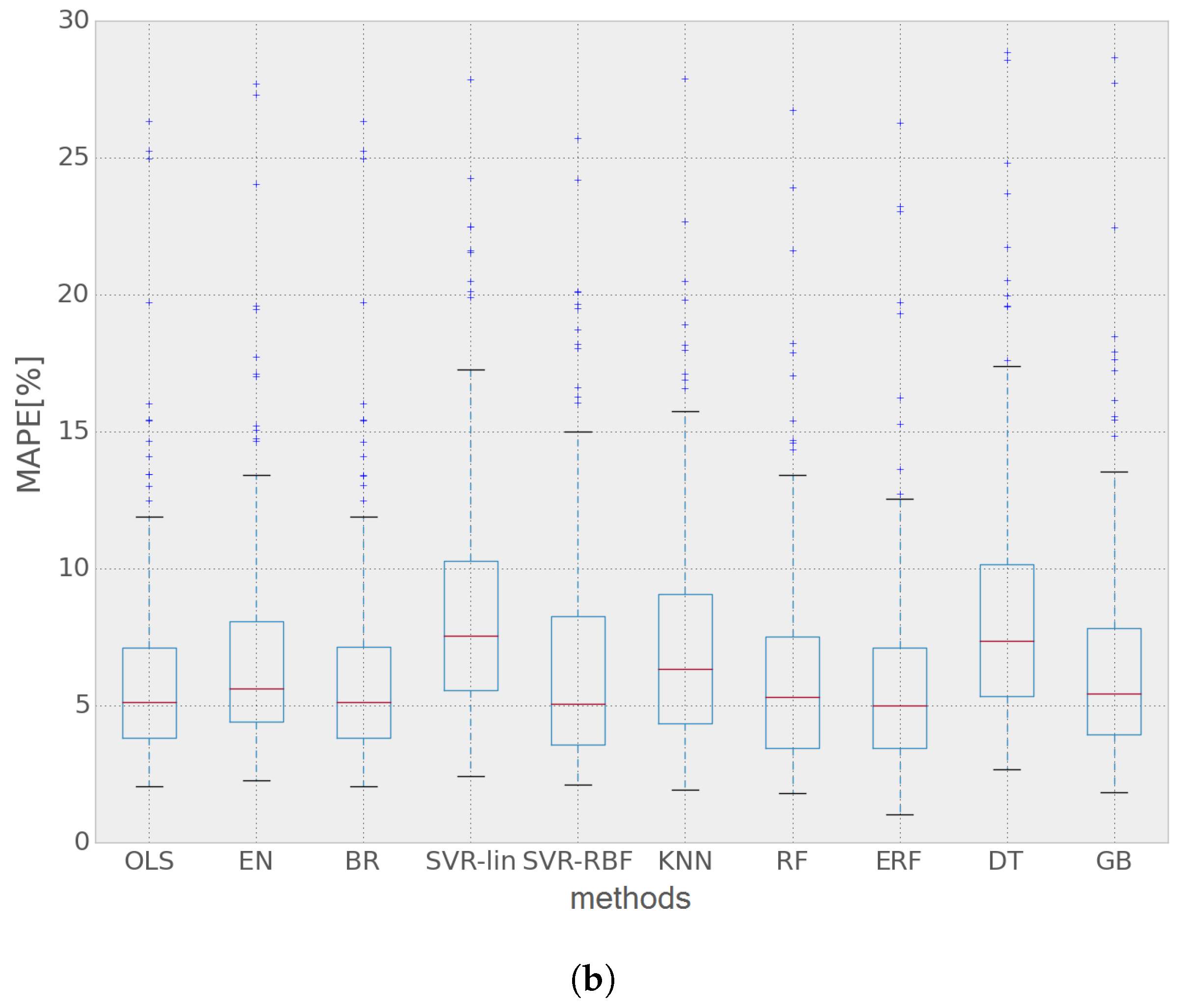
KNN	9206	4540

shows the results using the full feature vector. The feature vector is made up of hourly lagged load measures, lagged temperature measures, the week of the day of the sample to be forecasted and the hour of the day, i.e., $x=x_l(168)\parallel x_c\parallel x_m(24)$. Some non-linear models, such as SVM using a linear kernel and DT, overfit the model on the training data of both networks, exploiting some relationships between features that are not present anymore in the test dataset. EN shows the best performance for Network 1; whereas ERF has the lowest MAPE for Network 2. The latter has better results overall, which is to be expected since it has a higher level of aggregation (as has been said before, Network 1 comprises 63 customers, while Network 2 is composed of 433 customers), which results in lower load demand variability. Moreover, Network 1 is entirely composed of household customers; whereas Network 2 has both household and commercial clients. It may be observed that EN gives the best performance for Network 1; whereas six other methods perform better for Network 2, which could mean that EN is a better option when most of the network is composed of similar type customers (i.e., residential). Similarly, ERF has the lowest MAPE value for Network 2; whereas it does not perform as good for the Network 1 dataset.

4.3. Discussion

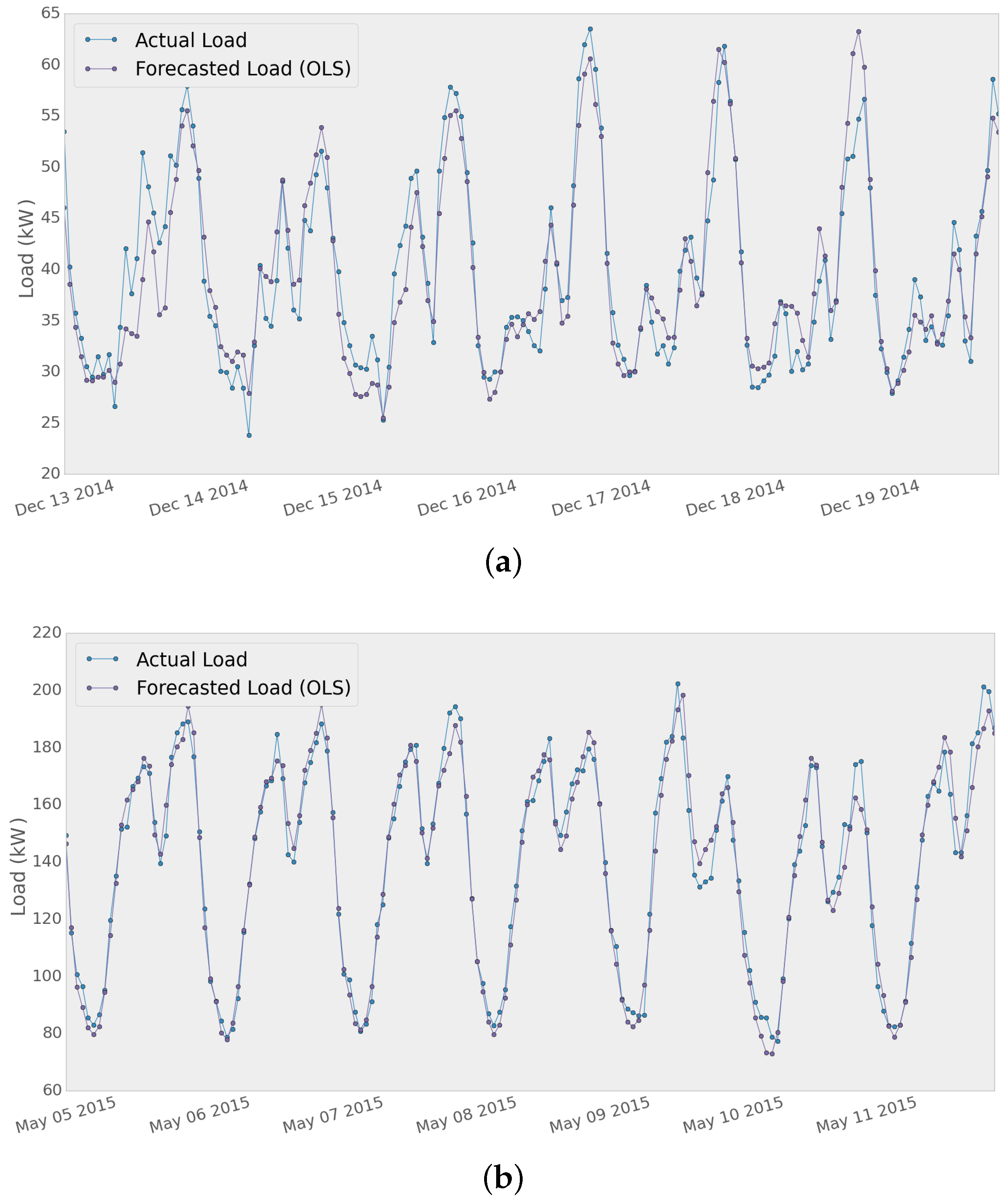
A sample of the results for the two different time series using the OLS method is shown in Figure 9. The forecasting model was fit using the training set and then tested for seven days, generating seven 24 h-ahead forecast profiles. Then, the MAPE, MAE and RMSE metrics were extracted from the results, and the average of the error metrics for that period of time was calculated as shown in

Table 3. MAPE, MAE and RMSE scores.

	MAPE		MAE		RMSE
	Network 1	Network 2	Network 1	Network 2	Network 1	Network 2
OLS	6012	3310	2476	4721	3060	5876
EN	5392	3775	2226	5421	2784	6736

.

The results presented in Table 3 show the performance of the OLS and EN models for both networks. It can be seen that the MAPE score is better for Network 2, which can be due to the fact that Network 2 data are formed by the aggregation of 433 smart meter measurements (433 customers as opposed to the 63 customers connected to distribution power Network 1). Moreover, the Network 2 dataset contains a mixed group of commercial and household customers, which could lead to a lower variability of the measurements and a better performance of the models.

The presented results show that the error values obtained using the different methods have an important variability throughout the year. In Figure 10 it can be seen that some of the 24 h-ahead predictions have around 1%–3% MAPE for Network 1 and 1%–2% for Network 2; whereas sometimes, these values reach 30%–40% and 20%–30%, respectively.

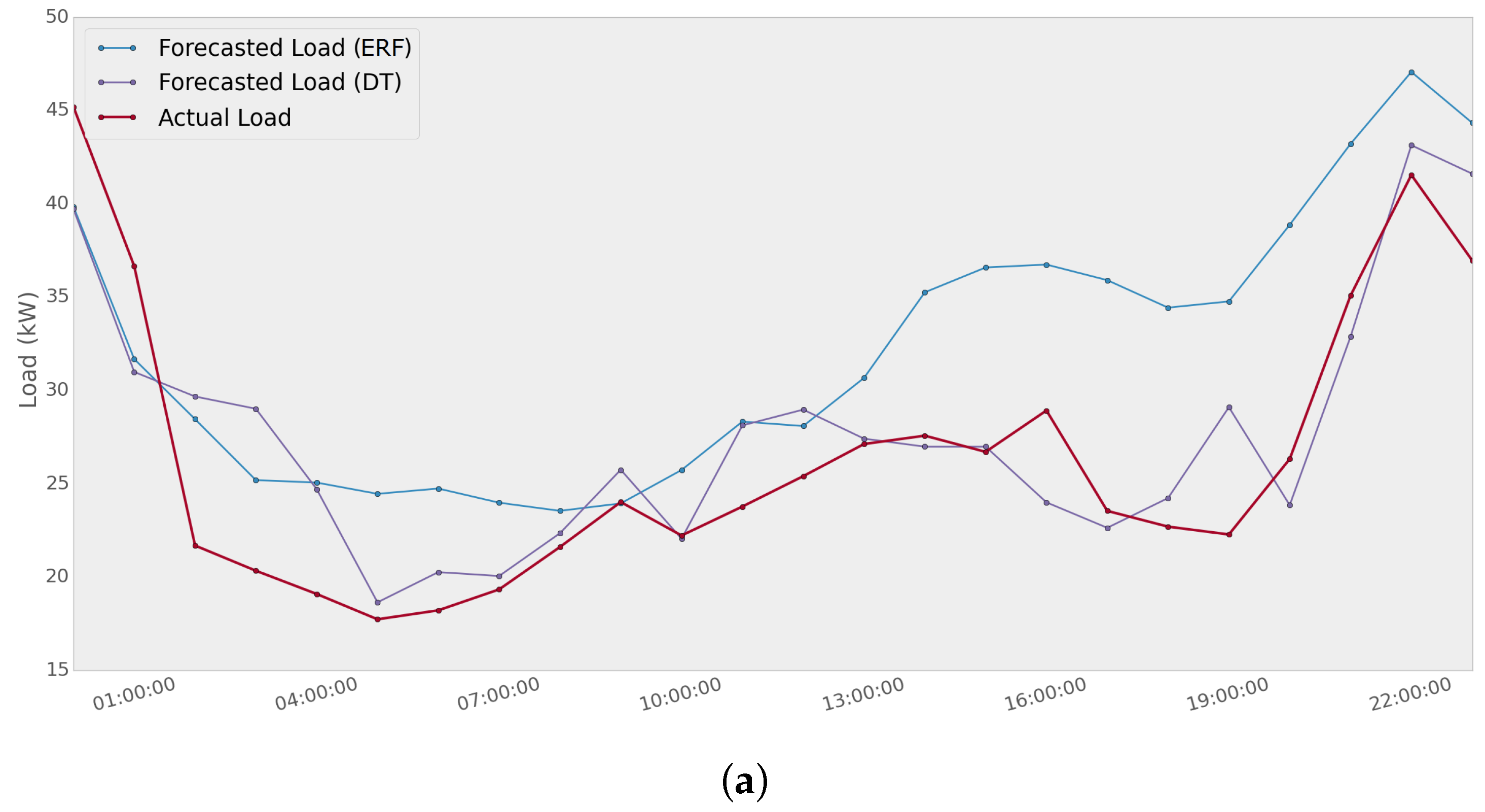
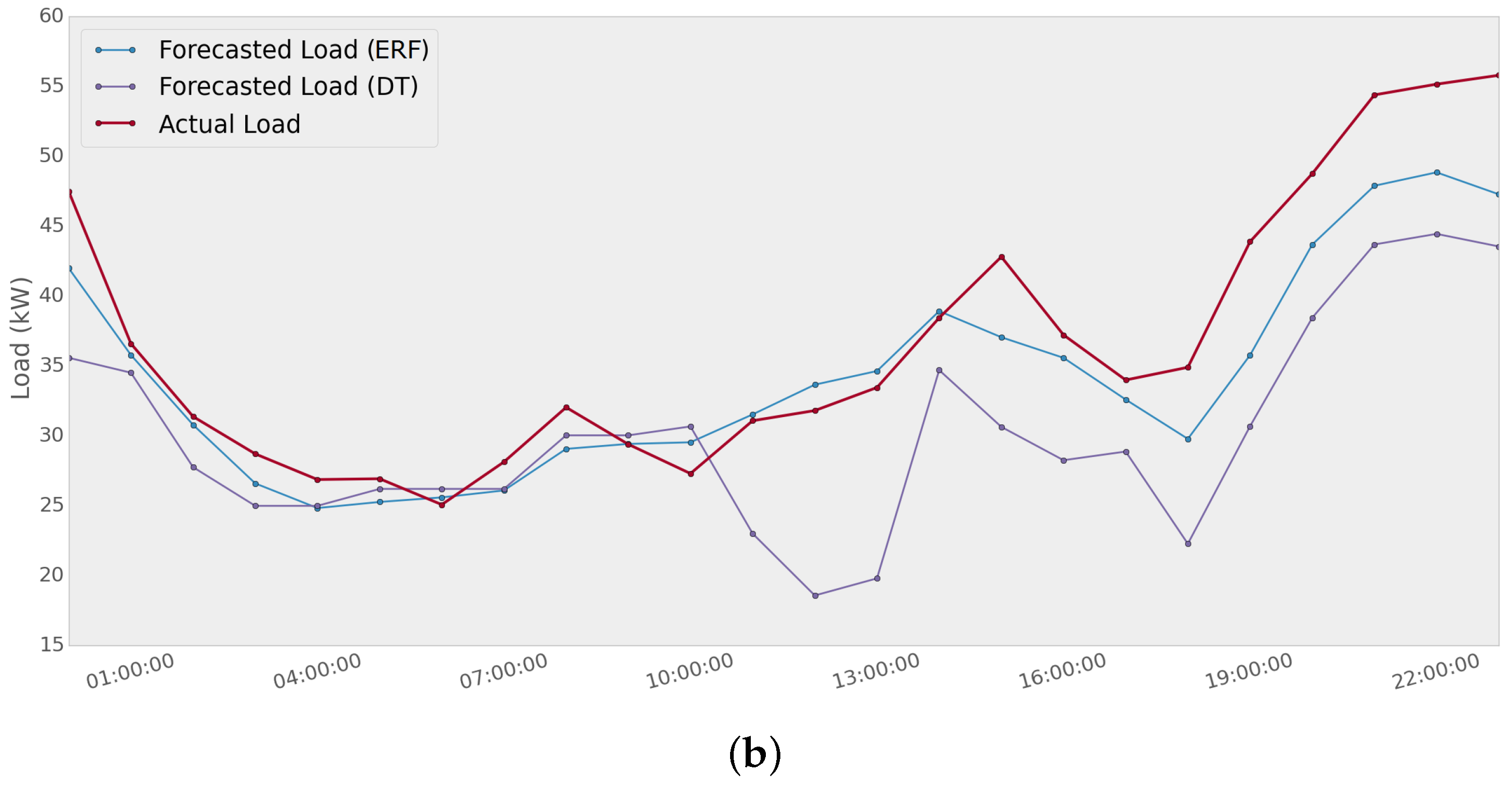
In Figure 11, an example of how two different methods present a significant variability is shown. Extremely randomized forest and decision tree methods are used to predict the load of Network 1 for two different days. The MAPE scores for the first day are 25.4% and 11.8% using ERF and DT, respectively. For the second day, the error values are 7.2% using ERF and 17.2% using DT. It can be noted that a single method provides good performance for a specific day; whereas the same method could have a poor performance a few days later.

5. Definition of an Adaptive STLF Methodology

From the previous results, it can be deduced that certain methods obtain the best performance when data are available throughout the whole testing period, but the error increases substantially when some of the data are corrupted or some data are missing due, for example, to communication problems in the smart grid deployments. On the other hand, other methods perform better when some of the data are missing or have to be discarded (i.e., the error increment is acceptable, as opposed to the other methods).

In order to overcome the variability in the performance of the different forecasting methods shown by the thorough analysis in the previous sections, an adaptive short-term load demand forecast methodology to improve the performance of the 24 h-ahead load demand predictions is proposed.

The adaptive short-term forecast is designed to predict electricity load demand in an autonomous way, automatically selecting the optimal short-term forecast method for the next h hours (forecast horizon). The adaptation is based on the optimization of the performance in previous periods by minimizing the prediction error. An iterative optimization is performed periodically, selecting the best forecasting method (and its parameters) for the following h hours. The core of the system is an iterative comparison of the errors generated by the different methods obtained in previous frames.

Given the entire electricity load of each dataset, data are divided into $N_T$ frames of variable length L (e.g., 24, 168 h). Each frame has to start on any day of the week (i.e., 00:00). For a period T of available historical electricity load, half of it ($T/2$) is used as a training sub-dataset. The other half is then classified into a validation set ($75\%$) and a testing set ($25\%$). The frames contained in the validation set ($N_V\in N_T$) will then be used by the proposed adaptive algorithm.

The adaptive STLF scheme is formulated as an M-method $N_V$-frame problem (where M is the set of methods previously discussed, and $N_V$ is the subset of frames contained in the validation set), in which an iterative comparison mechanism is used to minimize the MAPE among all $N_V$ frames to select the best method for the current forecasting day. First, an initial method-frame assignment is chosen for the whole validation dataset based on the optimization of the prediction error. The method-frame assignment algorithm is then adjusted in a number of iterations. During each iteration, each method’s performance is evaluated calculating its MAPE ${\epsilon }_m$ along the frame’s length L. The method that achieves the minimal MAPE, denoted as ${\epsilon }_{min}$, is then assigned to that frame. The optimization scheme goes as follows:

• Compute the $N_{V}xM$ matrix error E obtained from the validation sub-dataset:

  $$E=\left(\begin{array}{cccc}{\epsilon }_{11}& {\epsilon }_{12}& \cdots & {\epsilon }_{1M}\\ {\epsilon }_{21}& {\epsilon }_{22}& \cdots & {\epsilon }_{2M}\\ ⋮& ⋮& \ddots & ⋮\\ {\epsilon }_{N_{V}1}& {\epsilon }_{N_{V}2}& \cdots & {\epsilon }_{N_{V}M}\end{array}\right)$$

  (10)
• for $k=1:N_V$ do:

  2.1.

  Find the minimum element of each row of E, and denote them as ${\epsilon }_{1,min},\cdots ,{\epsilon }_{k,min}$. The number of rows in E is denoted as k. Each row k corresponds to a frame.

• Define forecasting date and horizon h for the current forecasting day.
• Select reference frame $k_{ref}$ to obtain the best method to forecast the following h hours. Different frames of variable length L can be considered as a reference to obtain the best method:

  (a)

  Frame A: The frame used as a reference corresponds to the previous 168 h. Once the best performing method from the previous 168 h is deduced, it is used for the whole upcoming week. In this case, the frame length $L=168$ h.

  (b)

  Frame B: The previous 24 h are selected as the reference frame, and the best performing method, from the previous 24 h, is used only for the following 24 h. The algorithm is updated daily, and the frame length $L=24$ h.

  (c)

  Frame C: Instead of evaluating the previous day (frame B), the same day from the previous week is considered as the reference frame (e.g., previous Monday). The obtained method is used for the following 24 h, and the algorithm is updated daily. Frame length $L=24$ h.

• Select method $M_{min}$ from matrix E that achieved the minimal error ${\epsilon }_{k_{ref},min}$ according to Equation (11).

  $${\epsilon }_{min}=\min (\sum _{m=1}^M({\alpha }_m\frac{1}{L}\sum _{t=1}^L\left|\frac{y_t-{\widehat{y}}_{t,m}}{y_t}\right|))$$

  (11)

  where ${\alpha }_m$ is the weight assigned to method m.
• Perform short-term load forecast using method $M_{min}$ to predict the next h hours

The forecasting methods considered in the adaptive algorithm are those presented in Section 3.2, and each one of them uses historical load demand and temperature measurements as input, as well as the forecasted temperature profiles for the next h hours (from the nearest meteorological station) and calendar information. The system proposed in this paper can be set to run automatically and might be used for any network that meets the following set of requirements:

• Enough historical hourly load measurements (at least one year).
• Temperature forecast available for the area (at least 24 h ahead with hourly resolution).

The selection of the most appropriate forecasting algorithm for a specific type of dataset can be considered an example of the classical algorithm selection problem, which has been studied over the last few years [35]. Lately, meta-learning techniques have proven to be very efficient selecting the most appropriate algorithm from a portfolio of multiple algorithms [36].

Meta-learning-based machine learning methods are automatic learning systems that are able to learn from past experiences (datasets and results of algorithms) to recommend the best algorithm for a current dataset [37]. Although the design of a meta-learning forecasting algorithm such as is shown in [16] is out of the scope of the paper, some comparisons between adaptive and meta-learning techniques are summarized next:

• One of the great advantages of meta-learning-based techniques is that they can give a solution almost immediately. On the contrary, the computing time required by an adaptive system increases with the number of algorithms included in the portfolio.
• Another advantage of meta-learning techniques is that they are able to recommend the best algorithm for a given dataset, whereas adaptive systems can provide, in some specific situations, suboptimal solutions (local-minima) and not the optimal or best ones.
• It has to be noted that the cost of building the adaptive forecasting model is very low, offering at the same time great flexibility to upgrade the number of new algorithms in the portfolio, which represents one of the great advantages of the adaptive-based techniques. In contrast, meta-learning techniques are not flexible enough to increase the portfolio size. The meta-learning model has to relearn whenever the portfolio changes or whenever new metadata are available expending many computational resources (computational time and stream of data) [38].
• A critical aspect related to the design of meta-learning model is the right selection of the meta-features [39,40,41], which makes the building of the meta-model a challenging task. The meta-features used for learning the meta-model affect the results of the meta-learning technique, and there is no consensus on how meta-features have to be selected for a certain problem; in some cases, the most successful meta-features can be computationally expensive [42]. Adaptive techniques, as the one proposed in this paper, offer great robustness to the selection of parameters in the design phase, being one of the more important advantages.

Implementation of the Adaptive Short-Term Load Forecast

The adaptive STLF algorithm is used to dynamically select the most optimal method for the upcoming hours (independent of the characteristics of the network, type and number of customers, amount of data and singularities of the day to forecast). This improves the performance of the meta-learning system, where the lowest error is equal to the lowest error of the load forecasting algorithm that proves to be the optimum one. In the implementation of the adaptive short-term forecast algorithm in Networks 1 and 2 of the OSIRIS smart grid deployment, the reference frame had to be selected as is described in the algorithm definition.

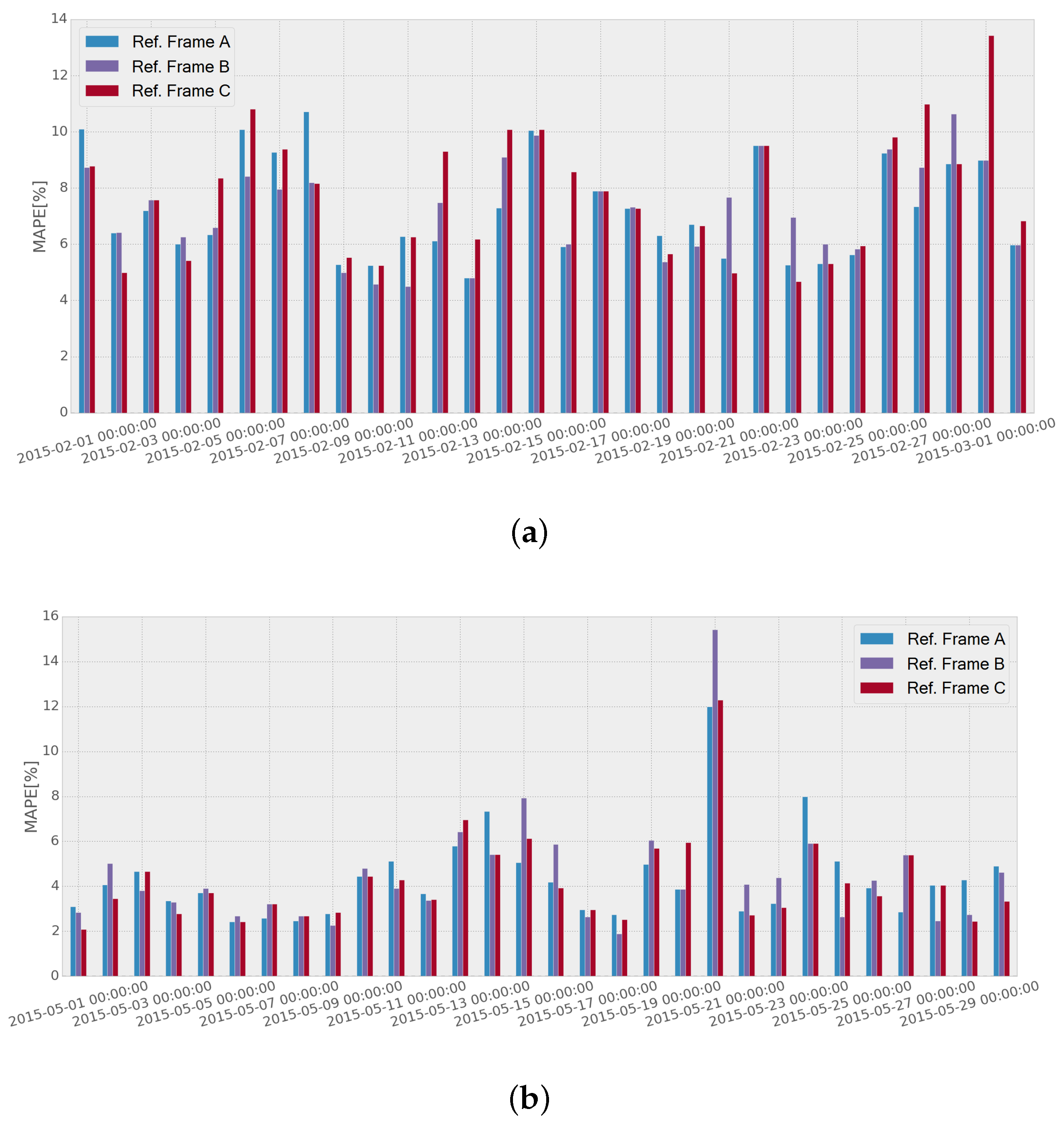
To evaluate which frame should be selected as $k_{ref}$, the adaptive short-term forecast was run using the three different reference frames previously presented. Figure 12 shows the performance comparison when using frames A, B and C, respectively, for four consecutive weeks. It can be seen that there is some variability in the performance when using different reference frames, although the errors tend to even out. The mean errors achieved through the testing month in Network 1 were $7.23\%$, $7.25\%$ and $7.75\%$ using reference frames A, B and C, respectively, which makes the difference between the three procedures not very significant. Similar results were obtained for Network 2: $4.35\%$, $4.46\%$ and $4.22\%$ using reference frames A, B and C, respectively. The results showed that the difference in the performance was not significant enough for the overall performance to single out each case, and hence, it was decided to select frame A as $k_{ref}$ to the whole of the tests, because it offers minimum mean error in Network 1, and the difference from the frame with the lowest error in Network 2 is not significant. In addition, it offers minimum computational complexity, as it only has to be updated weekly, and the same method is used for the whole week.

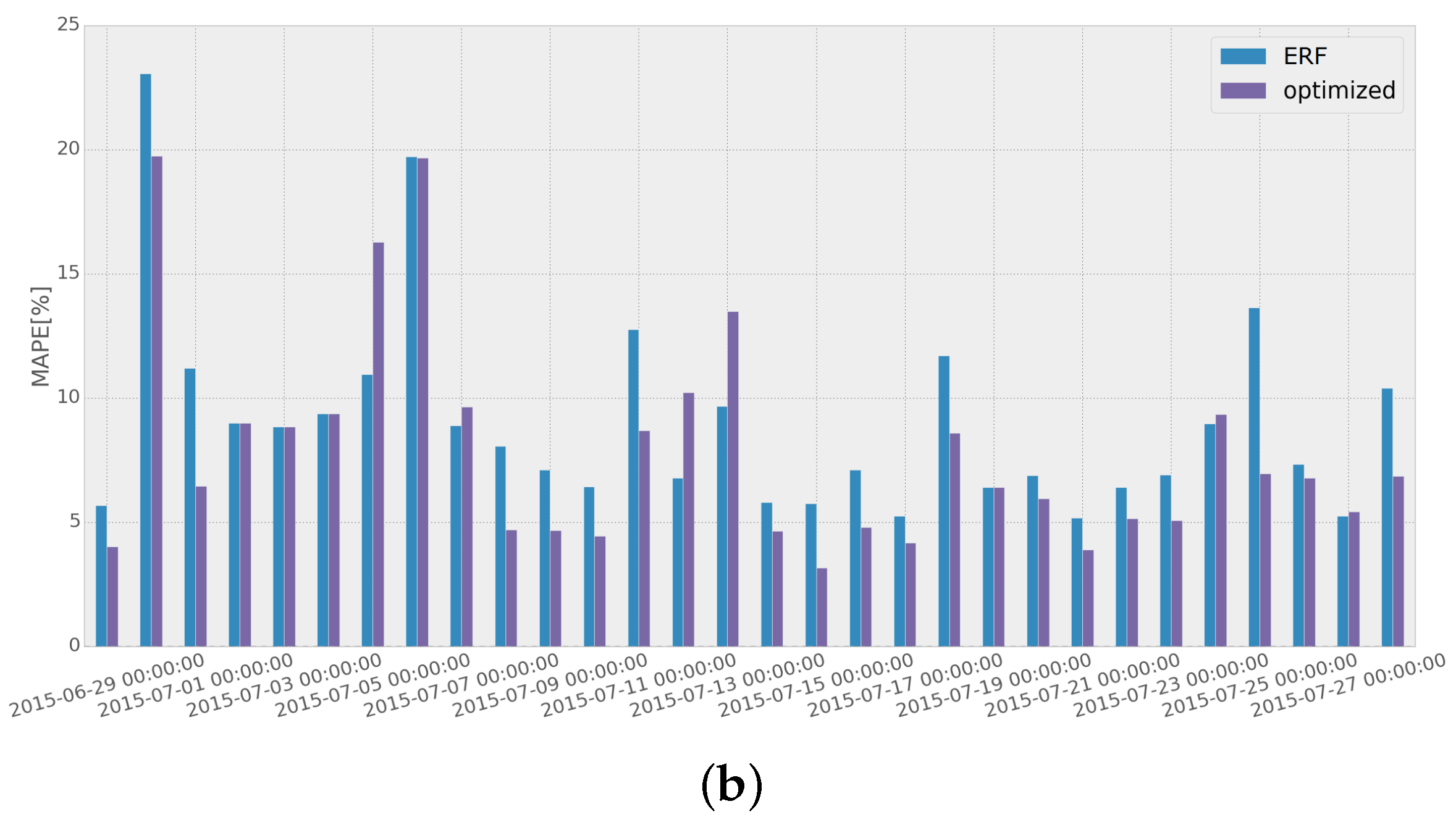
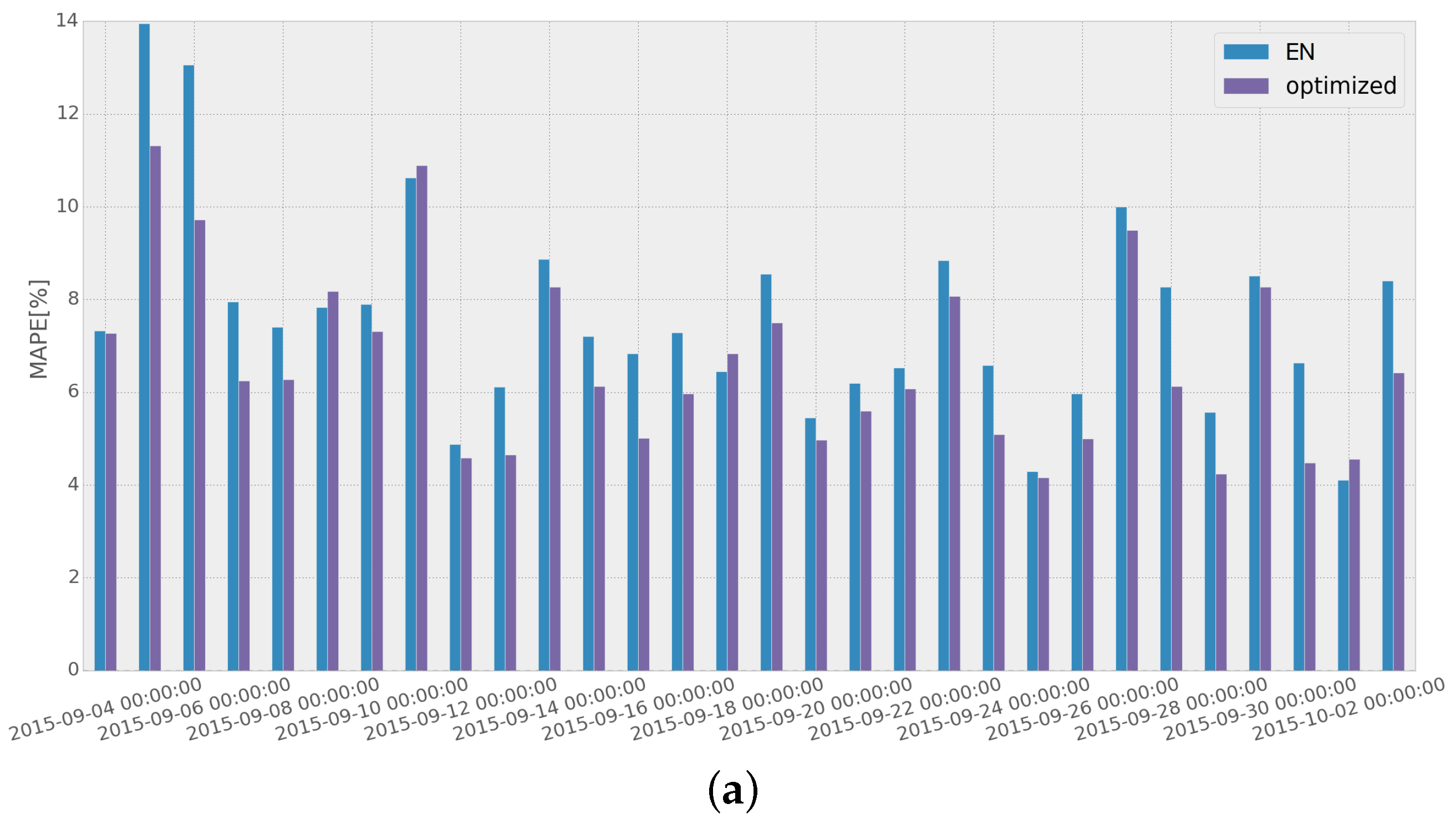
To assess the improvement obtained when the adaptive short-term forecasting algorithm is used, we compared the MAPE scores achieved with and without the implementation of the adaptive algorithm for a specific month, as has been presented in Figure 13. EN and ERF are used as the STLF methods for both networks (EN for Network 1 and ERF for Network 2), as they present the best overall performance throughout the whole test dataset (as was shown in Table 2 in Section 4.2).

Results show that using the adaptive load forecasting algorithm, the overall performance is improved. It should also be noted that in both networks, most of the highest error values are reduced considerably, resulting from removing the use of the methods that have been performing poorly in the recent days.

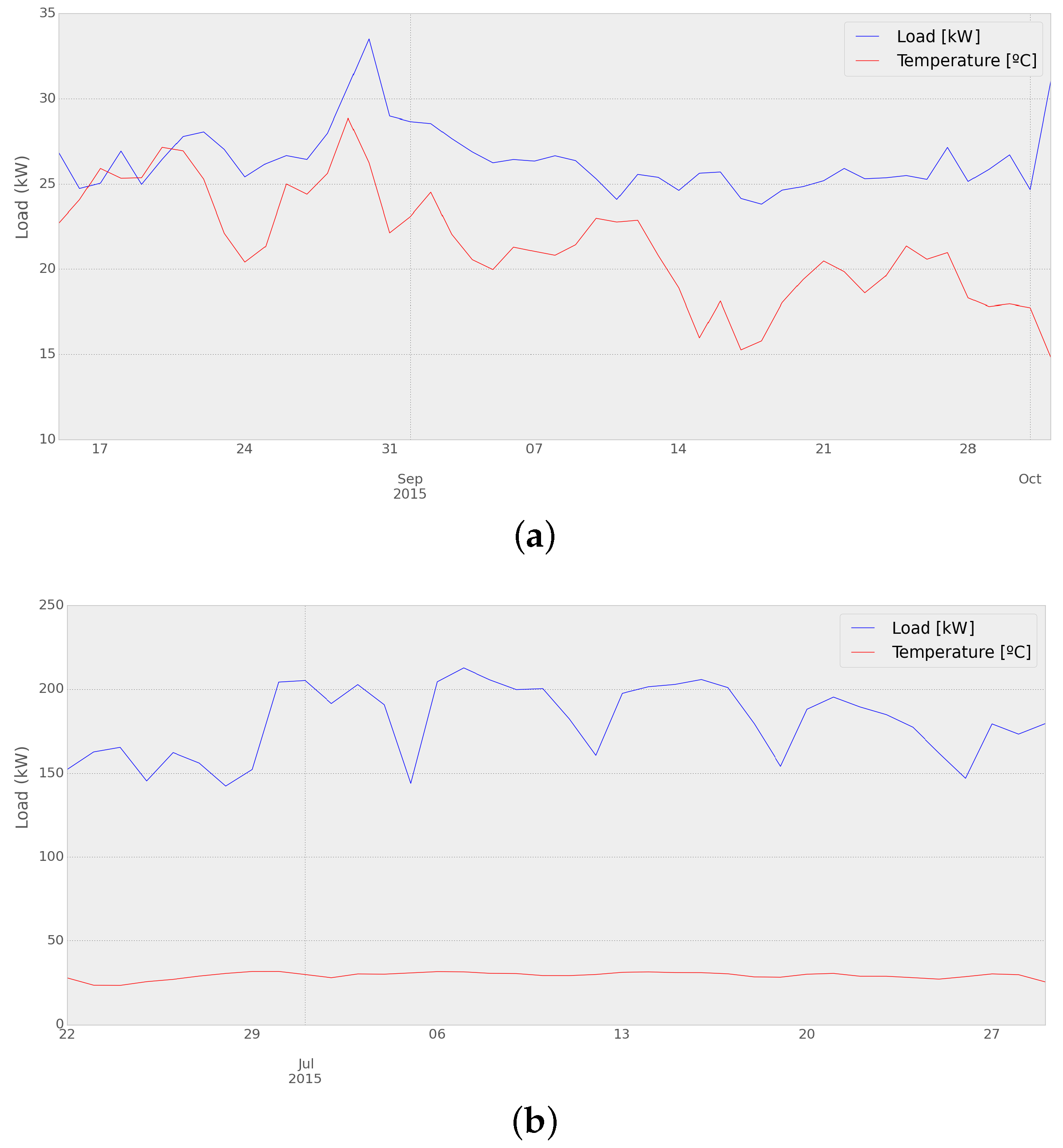
Some days present a higher error when using the optimized result. This could be explained for Network 1 by the temperature drop occurring the week previous to those days, as can be seen in Figure 14a. As for Network 2, it can be seen in Figure 14b that the week before the days with the lowest performance, the load curve presents an unusually low energy consumption, which would lead to a higher chance of error in the optimization process of the adaptive load forecasting methodology.

6. Conclusions

This paper presents the methodology used to select the best performing method for forecasting the electricity load demand in two existing distribution power networks of the OSIRIS Smart Grid demonstration project, focusing on the short-term forecast of aggregated data from two different power networks. It is important to realize that when working with data from an actual smart grid deployment, it is possible that some data are corrupted or missing due to communication problems in the smart grid monitoring system. The results presented in this paper show that some non-linear methods, such as SVM, with a radial basis function kernel or ERF (using 50 decision trees), reach their best performance with only 24 lagged hourly load measures, which could be useful when the availability of data is limited. Other linear methods, like EN, need at least 168 lagged load values to achieve its best performance. Regarding the number and type of customers that comprise the different networks, it is shown that some methods behave better when most of the network is made up of a similar type of customers (household, commercial or industrial). However, they fail when the aggregated data are composed by a mixed proportion of different types of customers. On the other hand, other methods, such as ERF, present the lowest prediction error when the data variability is lower, which is the case of power networks with a large number of customers, whereas they are not recommended to be used when the network is small and it is composed mainly by household customers.

The obtained results suggest that different methods should be used depending on the conditions of the network, availability and quality of the measurements, as well as the type of customers. Moreover, results show that the same method might achieve the best performance for a specific period of time, but it also might perform poorly a few days or weeks later. This leads to the conclusion that a single forecast method is not able to provide the maximum accuracy for any condition of the network, any set of customers (type and number) or for any day of the year.

As a solution to this issue, a novel adaptive load forecasting methodology is proposed in this paper, which automatically selects the forecast method that fits better to the specific day of the year, type of network and condition of the distribution network providing 24 h-ahead forecast with the lowest forecasting error. The adaptive load forecasting methodology is tested in an existing smart grid demonstration network, and the obtained results show that the adaptive short-term load demand forecast might be applied in other smart grid deployments where the load forecasting information is crucial for the correct operation of the distribution network; and the high variability of the customers makes the prediction errors highly variable with time. To the best of the authors’ knowledge, such an approach has not been explored in the existing literature, which makes this methodology a relevant contribution to the state-of-the-art.