Article

Development of a General Package for Resolution of Uncertainty-Related Issues in Reservoir Engineering

1
Department of Oil-Gas Field Development Engineering, College of Petroleum Engineering, China University of Petroleum, Beijing 102249, China
2
State Key Laboratory of Petroleum Resources and Prospecting, China University of Petroleum, Beijing 102249, China
3
State Key Laboratory of Shale Oil and Gas Enrichment Mechanisms and Effective Development, SINOPEC Group, Beijing 050021, China
4
Department of Energy and Resources Engineering, College of Engineering, Peking University, Beijing 100871, China
*
Author to whom correspondence should be addressed.
Energies 2017, 10(2), 197; https://doi.org/10.3390/en10020197
Submission received: 20 November 2016 / Revised: 31 January 2017 / Accepted: 2 February 2017 / Published: 10 February 2017

Abstract

:
Reservoir simulations always involve a large number of parameters to characterize the properties of formation and fluid, many of which are subject to uncertainties owing to spatial heterogeneity and insufficient measurements. To provide solutions to uncertainty-related issues in reservoir simulations, a general package called GenPack has been developed. GenPack includes three main functions required for full stochastic analysis in petroleum engineering, generation of random parameter fields, predictive uncertainty quantifications and automatic history matching. GenPack, which was developed in a modularized manner, is a non-intrusive package which can be integrated with any existing commercial simulator in petroleum engineering to facilitate its application. Computational efficiency can be improved both theoretically by introducing a surrogate model-based probabilistic collocation method, and technically by using parallel computing. A series of synthetic cases are designed to demonstrate the capability of GenPack. The test results show that the random parameter field can be flexibly generated in a customized manner for petroleum engineering applications. The predictive uncertainty can be reasonably quantified and the computational efficiency is significantly improved. The ensemble Kalman filter (EnKF)-based automatic history matching method can improve predictive accuracy and reduce the corresponding predictive uncertainty by accounting for observations.

1. Introduction

With the advancement of the quantitative modeling techniques in petroleum engineering, numerical simulations have become popular for describing subsurface flow characteristics and making predictions with respect to subsurface flow behaviors. Common numerical simulators, such as Schlumberger Eclipse, CMG and TOUGH2, are widely used in petroleum engineering to aid decision-making for oil extraction. The most severe challenge posed by the need to obtain accurate predictions of oil production in a reservoir lies in the various sources of uncertainties associated with a selected predictive model. The uncertainties may stem from the spatial heterogeneity of the formation properties caused by the complex geological process and insufficient measurements limited by technological and economic factors. The uncertainty-related issues appear in two essential processes required by a complete reservoir modeling project: forward modeling and inverse modeling.
The uncertainty-related issue in forward modeling processes is related to quantification of the prediction uncertainties and risks for a given numerical model with several uncertain parameters [1,2,3]. Monte Carlo simulation (MCS) is the most widely used uncertainty quantification method. It has been applied to petroleum engineering and groundwater hydrology [4,5,6,7,8]. MCS requires generating a large number of realizations of the random inputs in order to obtain a reasonably converged result [1], which is achieved with a high computational cost. This cost may become unaffordable in some cases, especially when each simulation is already time-consuming. In recent years, a surrogate model-based method, called probabilistic collocation method (PCM), has been developed by some researchers [3,9]. The PCM method consists of two parts, the representation of the random variables using polynomial chaos basis and the derivation of the appropriate discretized equations for the expansion coefficients on selected collocation points. This method was applied to the fields of petroleum engineering and groundwater hydrology [10,11] to estimate predictive risks.
Inverse modeling, also known as data assimilation or history matching, aims to reduce the predictive uncertainty through model calibration assisted by the production data. Traditional inverse modeling process is implemented by hand so that the simulation output can match the production data well, and the performance of the calibration results strongly depends on engineer experience. However, this traditional inverse modeling method is inefficient and sometimes infeasible for application in complex models with a large number of parameters. Many automatic history matching methods have been developed recently [12,13,14,15]. Attributing to the development of the in-situ monitoring techniques, a sequential stochastic inversing modeling method, the ensemble Kalman filter (EnKF), attracts a lot of attention. Apart from its conceptual simplicity and easy implementation, the following factors support the popularity of the EnKF method: (a) it is a non-intrusive method, which can be integrated in a straightforward manner with already available simulators; (b) it allows the flexibility to provide the uncertainty associated with the system states at each assimilation step; and (c) it can be extended to enable us to handle a large number of parameters to characterize subsurface flow systems under uncertainty [16,17,18,19,20,21]. The EnKF procedure is composed of two stages: the forecast stage and the assimilated stage. The field is first parameterized and represented by a set of realizations in terms of prior knowledge. In the forecast stage, the model response of each realization is propagated forward in time. In the assimilated stage, the parameters of each realization are updated by assimilating available observations [16]. The successful use of EnKF in various areas has been reported in many literatures [22,23,24,25].
Since uncertainty-related issues are ubiquitous in petroleum engineering, there is an urgent need to develop a software package that has the capability to integrate various state-of-the-art stochastic forward and inverse modeling methods and conduct a complete stochastic analysis to aid the decision-making for a given project. Here, we develop a general package, named GenPack, to handle a comprehensive set of the uncertainty-related issues. To our knowledge, no similar software package has been developed in the petroleum engineering field. The innovations of our developed GenPack are that: (a) it is programmed in a modularized manner and can be extended easily when new functions are required; (b) it is customized to petroleum engineering applications and is ready to be integrated with any existing simulator, thus it can be easily implemented by petroleum engineers; (c) theoretical analysis methods, such as probabilistic collocation method and parallel computing techniques, are both used to tackle the obstacles regarding computational efficiency in stochastic analysis. The purpose of GenPack is to facilitate the implementation of stochastic analysis required by either researchers or engineers, and it also provides a platform to easily integrate with other functions when new methods are created. This package is freely available upon request (https://www.researchgate.net/publication/313114201_GenPack_Code).
This paper is organized as follows. Section 2 illustrates the theoretical bases required in the developed general software package. Section 3 is devoted to demonstrating the capability of the package to quantify uncertainty and implement automatic history matching. Conclusions are presented in Section 4.

2. Methodology

The developed GenPack software includes three main features. These features are the generation of the random parameter field, the stochastic forwarding modeling to quantify the predictive uncertainty, and automatic history matching to calibrate the numerical model against the sequentially available data. The methods selected to achieve the desired features are either widely accepted (e.g., sequential Gaussian simulation method and the ensemble Kalman filter method) or performed well based on our research experiences (e.g., the Karhunen–Loeve expansion method and probabilistic collocation method). In this section, the theoretical bases of all these built-in methods are introduced.

2.1. Random Field Generator

To characterize the heterogeneity of geological parameters, such as permeability and porosity, it is common to treat these parameters as Gaussian random fields. GenPack provides two options to generate the Gaussian random field, sequential Gaussian simulation method and Karhunen–Loeve (KL) expansion.

2.1.1. Sequential Gaussian Simulation Method

Gaussian sequential simulation method [1] is based on conditional probability density function (PDF),
p ( k 1 , k 2 , , k n ) = p ( k 1 , k 2 , , k n 1 ) p ( k n | k 1 , k 2 , , k n 1 ) = = p ( k 1 ) p ( k 2 | k 1 ) p ( k n | k 1 , k 2 , , k n 1 )
where k n denotes the parameter value at the location x n , i.e., k n = k ( x n ) .
According to the first part of Equation (1), an n-dimensional joint PDF of p ( k 1 , k 2 , , k n ) can be expressed by the product of an (n − 1)-dimensional conditional PDF and an unconditional PDF. If we keep re-iterating this process, we can obtain the final form of Equation (1). This equation indicates that we can generate a trajectory of (n − 1) parameter values, i.e., k 2 , , k n by taking advantage of the successive form of the conditional probability relation, once the first one is randomly drawn from the unconditional Gaussian PDF p ( k 1 ) with the known mean and variance of the field. The mean and variance of the conditional PDF following a Gaussian distribution can be determined by:
k ( x n ) c = k ( x n ) + i = 1 n 1 a i ( x n ) [ k i k ( x i ) ]
V a r c [ k ( x n ) ] = σ k 2 ( x n ) i = 1 n 1 a i ( x n ) C k ( x i x n )
where superscript c stands for conditional, and σ k 2 ( x n ) and C k ( x i x j ) are variance and covariance of geological parameter k ( x n ) , respectively.
The coefficients { a i ( x n ) } can be solved using the following equation:
j = 1 n 1 a j ( x n ) C k ( x i x j ) = C k ( x i x n ) , i = 1 , , n 1

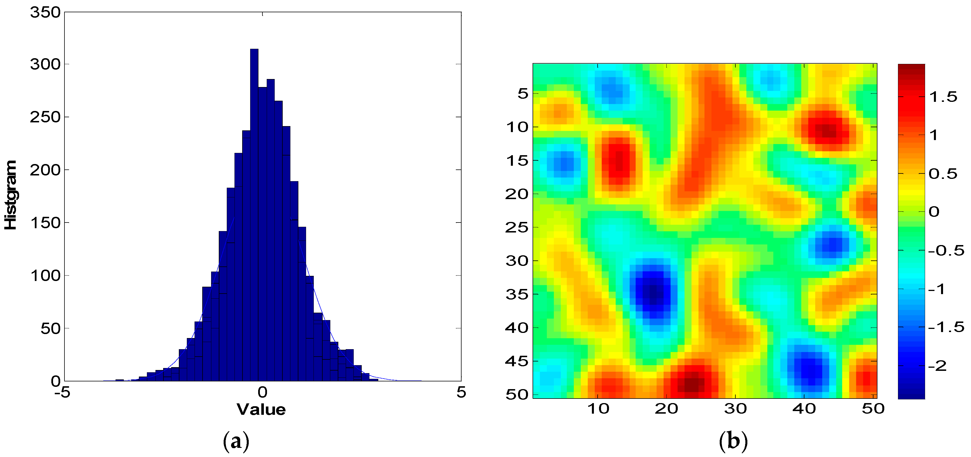
2.1.2. Karhunen–Loeve Expansion

KL expansion [10] is an alternative method to generate a random field. Let k ( x , θ ) be a random space function, where x D and θ Θ (a probability space). We have k ( x , θ ) = k ( x ) + k ' ( x , θ ) , where k ( x ) is the mean and k ' ( x , θ ) is the random perturbation term. The spatial covariance structure of the random field can be described by the covariance function C k ( x , y ) = k ' ( x , θ ) k ' ( y , θ ) . It may be decomposed as:
C k ( x , y ) = n = 1 λ n f n ( x ) f n ( y )
where λ n and f n ( x ) are deterministic eigenvalues and eigenfunctions, respectively, and can be solved from the Fredholm equation numerically:
D C k ( x , y ) f ( x ) d x = λ f ( y )
Then, the random field can be expressed as:
k ( x , θ ) = k ( x ) + n = 1 λ n f n ( x ) ξ n ( θ )
where ξ n ( θ ) are Gaussian random variables with zero mean and unit variance. Equation (7) is called the KL expansion. In practice, we often truncate the KL expansion with a finite number of terms. The rate of decay of λ n determines the number of terms that need to be retained in the KL expansion, which defines the random dimensionality of the problem.

2.2. Forward Modeling Methods

GenPack provides two types of stochastic methods to quantify the predictive uncertainty in the forward modeling process: the MCS method and the PCM method. Since the MCS method requires evaluating the model with a large size of parameter realizations to achieve reasonable convergence, it is more suitable to a model which needs relatively less computational time for each run. For a time-consuming model, the MCS method may be infeasible to implement. In such case, the PCM method can be a better option. It is a surrogate model-based stochastic modeling method, which requires fewer model evaluations but may lose a certain degree of accuracy due to the approximation in the process of surrogate model construction. The GenPack is designed to offer the flexibility for the user to select the more appropriate method.

2.2.1. Monte Carlo Simulation

MCS [1] is a direct method to solve stochastic partial differential equations. Consider a numerical model,
Δ = f ( ξ 1 , ξ 2 , , ξ N p )
where ξ = ( ξ 1 , ξ 2 , , ξ N p ) represents uncertain parameters, and Δ is model output.
MCS can be implemented in four steps: (1) Generating a realization ξ n from sampling; (2) Carrying out the simulation with ξ n and obtaining the model output Δ n ; (3) Repeating steps 1 and 2 and obtaining N s realizations; (4) Post processing and calculation of the statistic moments with the following equations:
Δ = 1 N s n = 1 N s Δ n
V a r ( Δ ) = 1 N s n = 1 N s Δ n 2 ( Δ 2 )
MCS is a very flexible method that is suitable for handling problems with extremely complex geometric boundary conditions. However, MCS requires generating a large number of realizations of the random inputs in order to achieve converged results [1]. This property of MCS prevents it from applications to real-world reservoir simulations, even running one of such simulations can be computationally demanding.

2.2.2. Probabilistic Collocation Method

As an alternative to MCS, the model output variables can be expressed by polynomial chaos expansion, which was introduced by [26]. The output variable Δ in Equation (8) can be approximated with the following spectral expansion:
Δ ^ = i = 1 N c a i Ψ i ( ξ 1 , ξ 2 , , ξ N p )
where { Ψ } is the multi-dimensional orthogonal polynomials of input uncertain parameters ξ 1 , ξ 2 , , ξ N p . The original polynomial chaos expansion is based on the assumption that the input uncertain parameters follow a multivariate Gaussian distribution. The Hermite polynomials form the best orthogonal basis for Gaussian random variables [27]. Unfortunately, in reservoir models, the uncertain parameters are not limited to the Gaussian distribution. Xiu and Karniadakis [3] developed generalized polynomial chaos expansions to represent different types of input uncertain parameters. In this study, orthogonal polynomial chaos expansions are constructed numerically for arbitrarily distributed input uncertain parameters [28].
The coefficients in polynomial expansions are usually solved by the Galerkin method [29,30]. The significant disadvantage of this approach is that it leads to a set of coupled equations governing those coefficients. For this reason, the approach is hard to implement in reservoir simulations where governing equations are nonlinear partial differential equations. Probabilistic collocation method (PCM) [31] is introduced as an alternative approach to resolve the coupling issue. Considering the stochastic model of Equation (5), the output Δ is approximated by polynomial chaos expansion and the approximation is denoted as Equation (8). Let us define the residual R between the real output Δ and its approximate Δ ^ as:
R ( { a i } , ξ ) = Δ ^ Δ
where { a i } are the coefficients of polynomial chaos expansion and ξ is the vector of uncertain parameters.
In the probabilistic collocation method, the residual should satisfy the following integral equation [10,11]:
R ( { a i } , ξ ) δ ( ξ - ξ j ) P ( ξ ) d ξ = 0
where δ ( ξ - ξ j ) is the Dirac delta function and ξ j is a particular set of random vector ξ . The elements in ξ j are called the collocation points. Equation (13) results in a set of independent equations. By solving these equations, the coefficients of polynomial chaos expansion can be obtained. The number of coefficients in polynomial chaos expansion is N c :
N c = ( N p + d ) ! N p ! d !
where N p is the number of uncertain parameters and d is the degree of polynomial chaos expansion. It can be found that N c sets of collocation points are needed to solve all the coefficients. Selection of collocation points is the key issue in PCM. Li and Zhang [10] suggested that the collocation points can be selected from the roots of the next higher order orthogonal polynomial for each uncertain parameter. Obviously, compared with the MCS, PCM is computationally more efficient.
Once the coefficients of the polynomial chaos expansions are obtained, the polynomial of Equation (9) can be used as a proxy for the original model of Equation (5). With the proxy constructed, the statistical quantities of model outputs, such as mean and variance, can be evaluated by sampling methods. Since the proxy model is reduced to a polynomial form and it does not involve the inverse process when solving equations, it can be evaluated much more efficiently. In addition, unlike the Galerkin method, the PCM method is non-intrusive because it results in a set of independent deterministic differential equations and can be implemented with existing codes or simulators.

2.3. Inverse Modeling Method

GenPack chooses EnKF [16] as the unique option to do inverse modeling due to its wide usage and better performance in the petroleum engineering field. The key theoretical basis underlying a typical EnKF approach is introduced here. We start by considering a collection of Ne realizations of the state vector S:
S = { s 1 , s 2 , , s N e }
where superscripts in Equation (15) refer to the index identifying the realization associated with each vector s i . The entries of the state vector are given by the random quantities that characterize the model, ξ , the dynamic state variables, u , and the observation data, d o b s . Observations at time t and their true values are related by:
d t o b s = H s t t r u e + ε t
Here, the superscripts obs and true respectively stand for the observation data and the true (usually unknown) system state; measurement errors collected in vector ε t are assumed to be zero-mean Gaussian with covariance matrix R t ; matrix H is the observation operator, which relates the state and observation vectors. The EnKF entails two stages, i.e., the forecast and assimilation stage.
In the forecast step, each state vector in the collection of Equation (13) is projected from time step (t − 1) to time t via:
s t f , i = F ( s t 1 a , i ) ; i = 1 , 2 , , N e
where the operator F ( · ) in Equation (17) represents the forward numerical/analytical model used to describe the physical process in petroleum engineering; superscripts f and a indicate the forecast and assimilation stages, respectively.
In the assimilation stage, the Kalman gain, G t is calculated as:
G t = C t f H t T ( H t C t f H T + R t ) 1
where C t f is the covariance matrix of the system state. This matrix is approximated through the N e model realizations as:
C t f 1 N e n = 1 N e { [ s t f , n s t f ] [ s t f , n s t f ] T }
Each state vector in the collection is then updated as:
s t a , i = s t f , i + G t ( d t o b s , i H s t f , i )
The updated ensemble mean and covariance respectively are:
E ( s t a | d 1 : t o b s ) = 1 N e i = 1 N e s t a
C o v ( s t a | d 1 : t o b s ) = 1 N e 1 i = 1 N e { [ s i , t a E ( s t a ) ] [ s i , t a E ( s t a ) ] T }
where d 1 : t o b s is the vector of observations collected up to time t, d 1 : t o b s = [ d 1 o b s , , d t o b s ] T .

2.4. The Design of GenPack

GenPack is developed by the object-oriented language C++, and the code is designed in a modularized manner in order to be conveniently reused and extended. Figure 1 shows the structure of our package. We designed a data container called “data base”. It can be considered as the data center of the software package. All of the setup parameters and simulation results are saved in this class. The function modules are encapsulated as entities, and they can achieve data interaction with users through “data base”. There are three main function modules in GenPack, namely, random field generator, forward modeling and inverse modeling. The random field generator is an independent module. It can generate Gaussian random fields via the sequential Gaussian simulation method and KL expansion, which are required in forward and inverse modeling. The forward modeling module provides two methods, MCS and PCM, for uncertainty quantifications. PCM is an extended method of MCS and it requires an extra module to construct orthogonal polynomials. We applied EnKF as the unique option of inverse modeling in the current version of GenPack. Since EnKF is a MCS-based method, part of the code in this module is shared with MCS module. The forward and inverse modeling modules interface with the reservoir simulator by creating data files according to the file format of the widely-used Schlumberger Eclipse in the current version. Other simulators can also be interfaced with Genpack by rewriting the Input/Output functions.

3. Results and Discussions

Several test cases corresponding to every module in GenPack are designed to illustrate the accuracy and efficiency of the GenPack in reservoir simulations.

3.1. Random Field Generation

If the key statistical attributes of the random log permeability field are known, we can take the covariance function of log permeability [1] as:
C o v ( x , y ) = σ 2 exp [ | x 1 y 1 | η 1 | x 2 y 2 | η 2 ]
Here, x = ( x 1 ,   x 2 ) and y = ( y 1 ,   y 2 ) are two spatial locations; σ 2 is the log permeability variance, which is set to unity in our demonstrative study; and η 1 and η 2 are the correlation lengths parallel to x 1 and x 2 directions in the Cartesian coordinate system, respectively. The values are set as η 1 = η 2 = 4 in this case.
We first apply KL expansion to generate the random log permeability field. To obtain a balance between computational accuracy and cost, we only retain the leading terms in the KL expansion, i.e., those terms with the largest eigenvalues. Figure 2 and Figure 3 show the results of KL expansions with 1000 and 100 leading terms, respectively. Histogram of the generated log permeability values are also given in these figures, which follow Gaussian distribution. More leading terms contained in KL expansion will provide more details of the random field. The field with 100 truncated leading terms only captures the main pattern of the field.
Sequential Gaussian simulation method is much more suitable for large model generation than KL expansion. It can be accelerated by parallel computing since each generation trajectory of log permeability realization is independent of the others. Figure 4 depicts a large 3D log permeability field (permeability along x direction, denoted as PERMX) generated via Sequential Gaussian simulation method provided by GenPack. This model has 80 × 80 × 80 = 512,000 cells. The computational time for running the simulation to generate the random field is 16.185 s with a single core (2.66 GHz Intel core and 2G Memory), which is comparable to geostatistical software library (GSLIB) [32]. With the parallel computing function switched on, the computational time is reduced to 4.521 s using all the eight cores on the same computer. The speedup, defined as the ratio of the sequential computational time to the parallel computational time, is almost 3.6.
The corner grid system is often applied to the reservoir model with a complex geometric boundary. To further improve the applicability of GenPack in petroleum engineering, the module of the sequential Gaussian simulation method is designed for random field generation in a corner grid system. The traditional GSLIB package to generate the random field does not have such capability, and may need an extra post-processing code to achieve this function. Figure 5 illustrates a porosity field generated in a corner grid.

3.2. Uncertainty Quantification

Sequential Gaussian simulation and KL expansion can be used to describe and characterize the random parameter field in GenPack. However, it is more important to know how the uncertain parameters may affect the flow behavior so that we can make rational decisions on the adjustment of the oil production process. A synthetic reservoir simulation case is designed to validate the uncertainty quantification module in GenPack. Both direct Monte Carlo Simulation method (i.e., MCS) and its surrogate model-based variant (i.e., PCM) are investigated in the test case. As discussed before, the purpose of the PCM method is to improve the computational efficiency by reducing the original model evaluations, but the cost is that it may lose a certain degree of accuracy due to the approximation in the process of surrogate model construction. It is common to consider MCS with a reasonably large realization size as the basis of the stochastic analysis. The results from the surrogate model-based PCM method are compared against these obtained from MCS to validate its accuracy and efficiency.
The synthetic case is a variant of SPE1 comparative solution project with a size of 1000 × 1000 × 300 ft. It is divided into 10 × 10 × 3 grids. A producer and injector are located in (10, 10, 3) and (1, 1, 1) respectively. A constant gas injection rate of 100,000 Mscf/day and a constant oil production rate of 20,000 stb/day for the producer are assumed. There are four uncertain parameters depicted in Table 1. These parameters are assumed to be uniform.
Figure 6 and Figure 7 depict the uncertainty quantification results of the BHP (bottom hole pressure) of the injector, and the producer´s BHP obtained from MCS and PCM respectively. It can be seen that the mean values of injector BHP and producer BHP yielded by the second-order PCM with 15 model evaluations and fourth-order PCM with 70 model evaluations can agree well with those obtained by the MCS with 1000 model evaluations. The variances provided by the second-order PCM have some deviations from the MCS results; however, the variances obtained by the fourth order PCM correspond with the MCS results very well. This indicates that the proxy constructed by the fourth order PCM is more reliable than that of the second-order PCM since the fourth-order PCM requires more collocation points, and uncertainty quantification analysis can be performed on the basis of the fourth-order PCM. It is noted that both the second-order PCM and the fourth-order PCM are much more efficient than the MCS method, e.g., the second-order PCM is almost 66 times faster than MCS and the fourth-order PCM is approximately 13 times faster than MCS. In general, higher-order PCM performs better than its lower-order counterpart in terms of accuracy, but it requires more original model evaluations as the number of collocation points increases. GenPack offers the option to use any order of PCM chosen by the user. A trial-and-error analysis can be performed by user to choose the best balance between accuracy and efficiency.
As can be seen in the theoretical basis, the MCS and PCM methods require multiple independent simulations to obtain the statistic moments. The time-consuming part of the uncertainty analysis is that of the simulations to evaluate all the statistical realizations. The independence of each realization makes these methods convenient for implemention with parallel computing. Each realization can be distributed to multiple Central Processing Unit (CPU) slave cores and then the results are collected by the master core to calculate the statistic moments. Figure 8 compares the CPU time of implementing an MCS uncertainty quantification case (25,000 cells) with 1000 realizations by using the single-core and the eight-core CPU on the same computer. It seems that parallel computing can be twice as efficient as sequential computing in this case.

3.3. History Matching

History matching method provides a means to constraint the model parameters by using observation data and thus can reduce the predictive uncertainty of the simulation model. GenPack allows the user to apply the EnKF method to implement the inverse modeling process. We will validate inverse modeling module in GenPack based on the test case described in the previous sections. The model parameter values used in the synthetic reference case are listed in Table 2. The synthetic observation values, i.e., the producer BHP values and the injector BHP values ranged from 100 to 900 days, and are generated based on the reference model. The EnKF method is then carried out to match the observations by optimally adjusting the model parameters. During the data assimilation process, the ensemble size is set as 50, and the assimilation step is 50 day. Figure 9 depicts the comparisons of the true values and initial realizations of model parameters before history matching. As shown in Figure 9, the 50 initial realizations of model parameters deviate from the true values significantly. It indicates a relatively poor initial estimate of the model parameters. Figure 10 depicts the mean predictions associated with their 95% confidence intervals (constructed using 50 prediction realizations) on the basis of the initial realizations of model parameters. The mean predictions deviate from the reference or true values dramatically even though the true values are within the envelope bounded by the upper and lower confidence intervals. Furthermore, the predictive variance represented by the width of the confidence intervals is relatively large, which indicates that there are relatively large uncertainties associated with the predictions.
After the history matching process, the model parameter realization values converge to the true parameter values much better, as shown in Figure 11. It seems that the permeability values in layer 1 and 2 as demonstrated in Figure 11b,c show relatively slower convergence compared with the porosity value and permeability value in layer 3, as demonstrated in Figure 11a,d. The reason may be that the permeability values in layer 1 and 2 are less sensitive to the observation data. Figure 12 depicts the predictions and their 95% confidence interval after history matching. As expected, the mean values of the predictions match the true value very well and the predictive variances decrease dramatically after history-matching. Since the EnKF method is a Monte Carlo-based method and the model evaluation for each parameter realization is independent of the others, it also can be accelerated via parallel computing.

4. Conclusions

This work can lead to the following major conclusions:
(1)
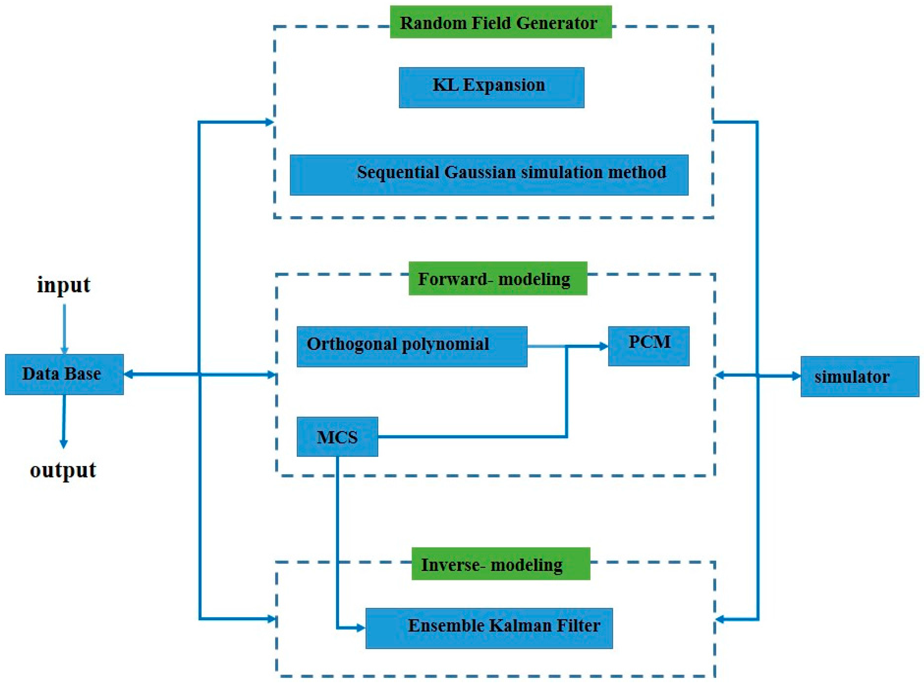
Uncertainty-related issues are extremely important to aid the decision-making process in petroleum engineering. It is imperative to develop an efficient tool to quantify the risks and calibrate the simulation models. In this study, we designed a comprehensive general package, named GenPack to integrate together uncertainty quantification in forward modeling and uncertainty reduction in inverse modeling. GenPack is a helpful tool for petroleum engineers and researchers to effectively investigate the uncertainty-related issues in practice. In the current version of GenPack, the selected methods are either widely accepted or performed well in the existing literature. Other methods can be incorporated when they become available due to the modularized design of this package.
(2)
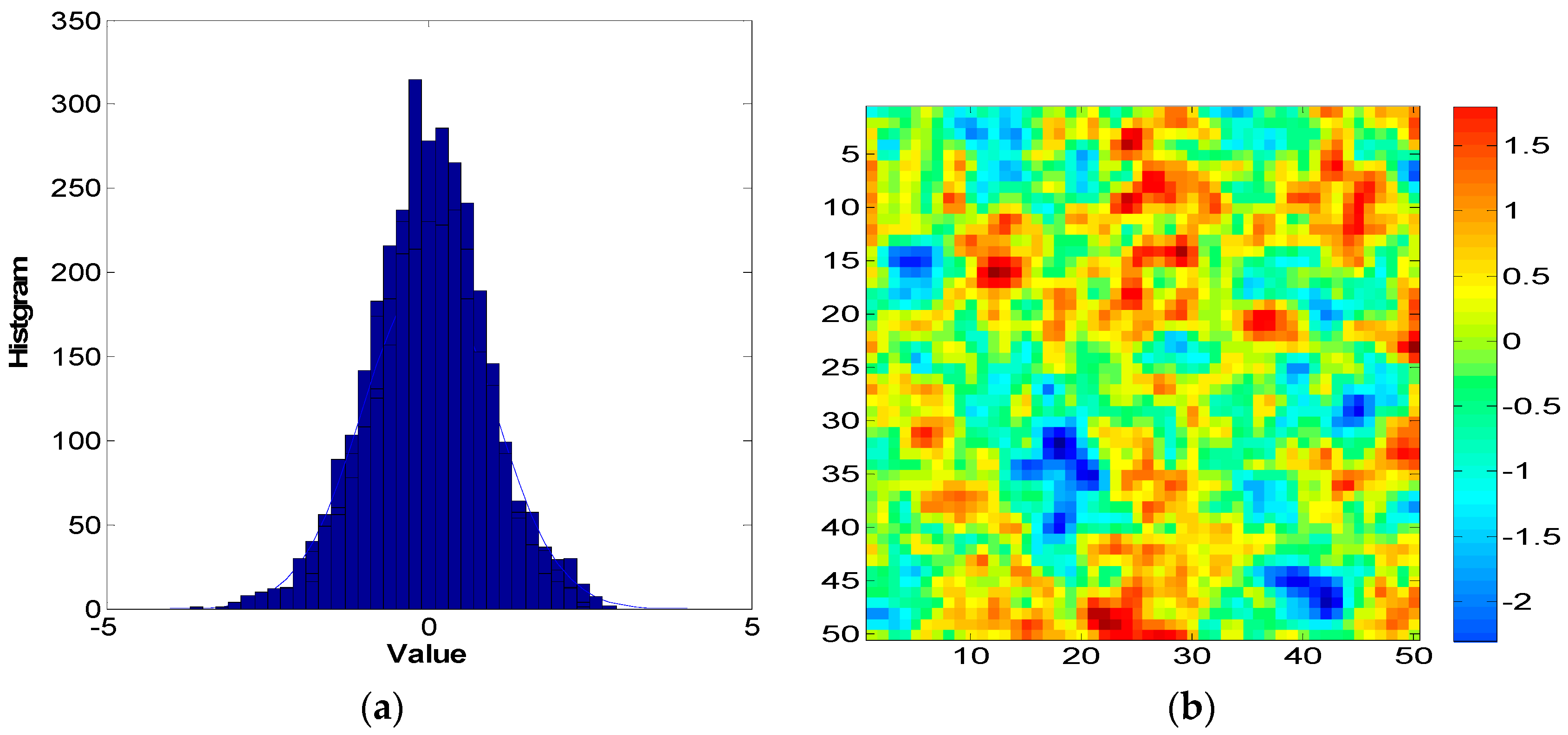
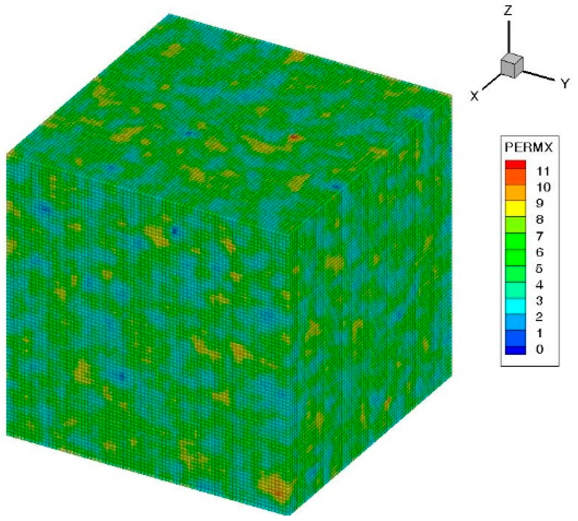
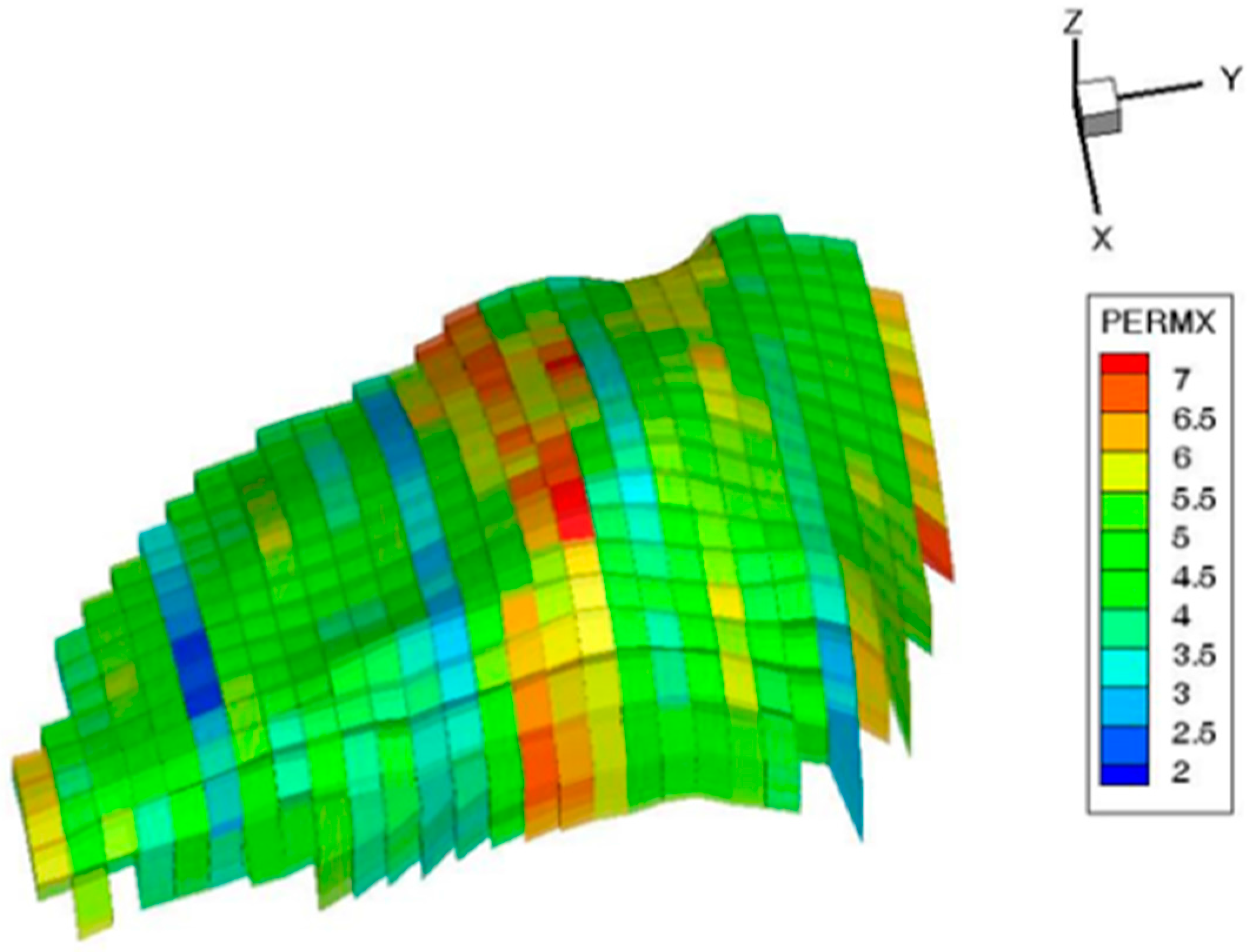
GenPack allow user to generate Gaussian random fields via either KL expansion or sequential Gaussian simulation method. In order to improve the computational efficiency, one should decide how many leading terms can be retained in KL expansion. Sequential Gaussian simulation method is found to be suitable for parameter field generation in a large model with complex geometric boundaries.
(3)
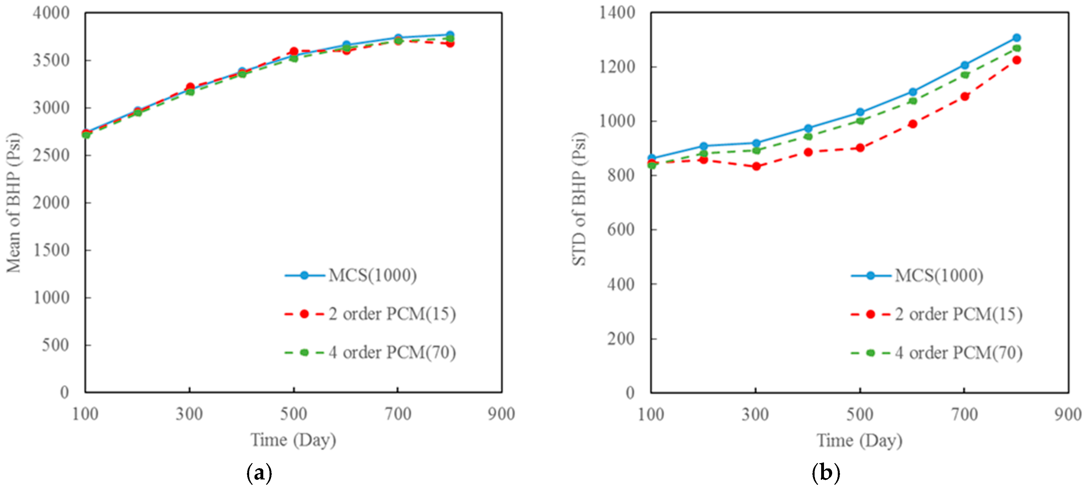
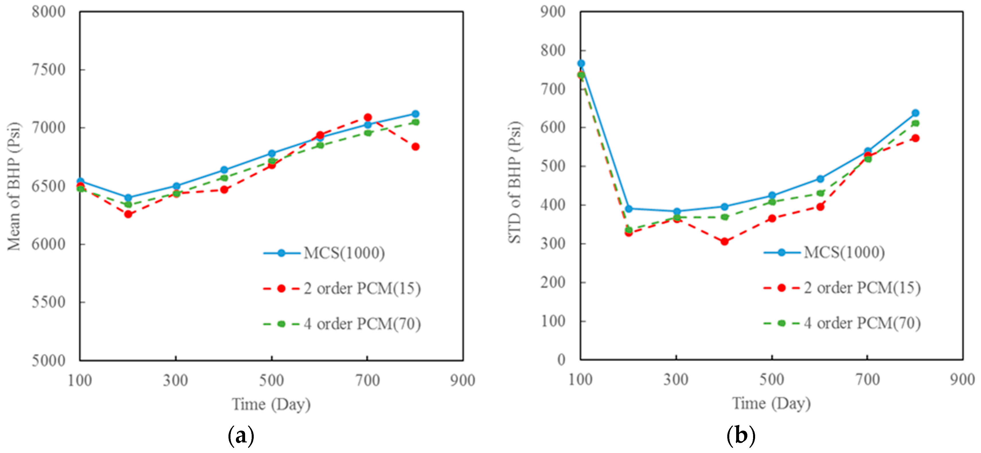
MCS and PCM are the options in GenPack to quantify uncertainty. MCS is a robust method for uncertainty quantification even though it requires large number of samples to guarantee the convergence. PCM is an efficient method to quantify uncertainty. The appropriate order of PCM can be investigated to achieve the balance between efficiency and accuracy during the analysis process.
(4)
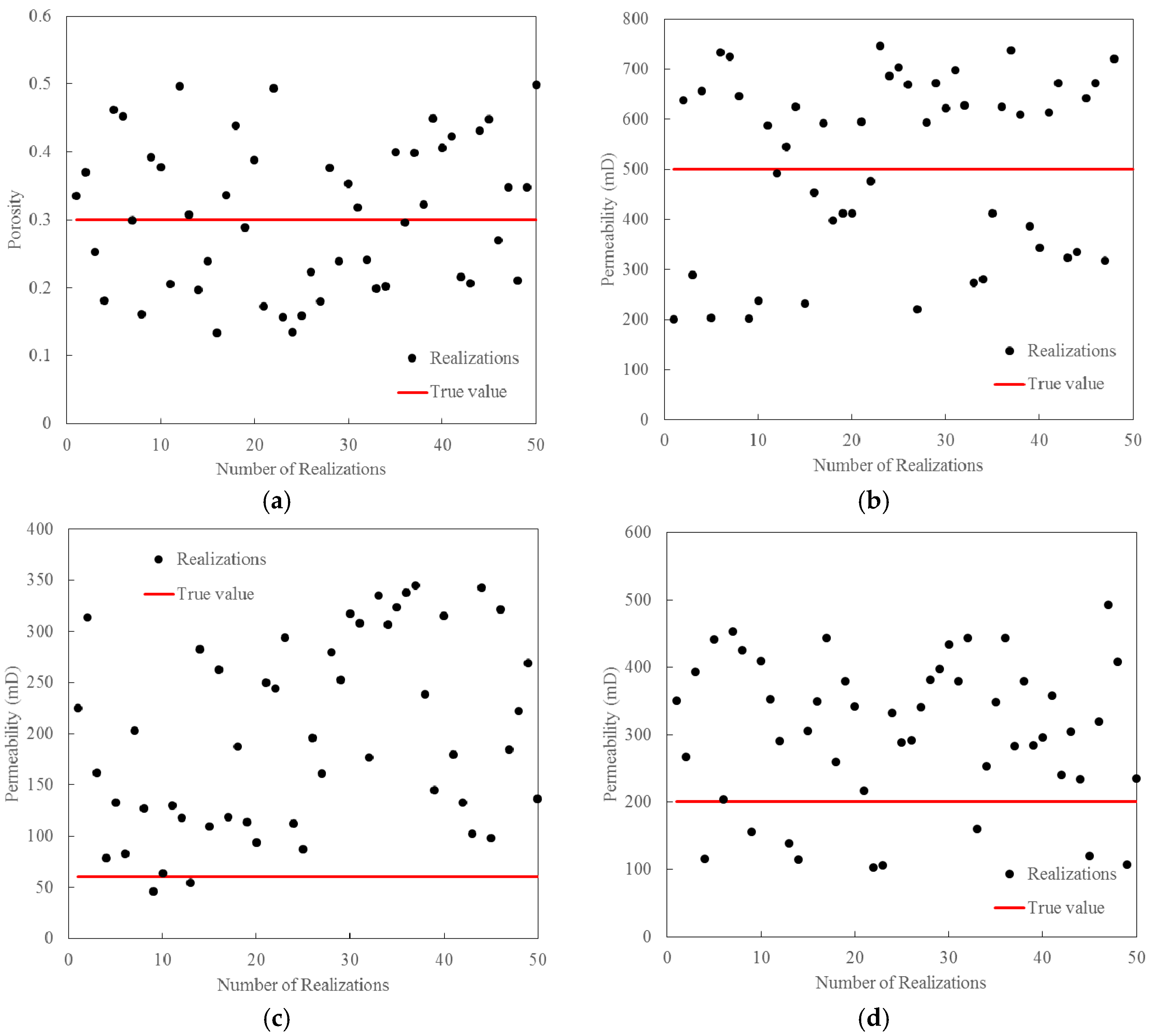
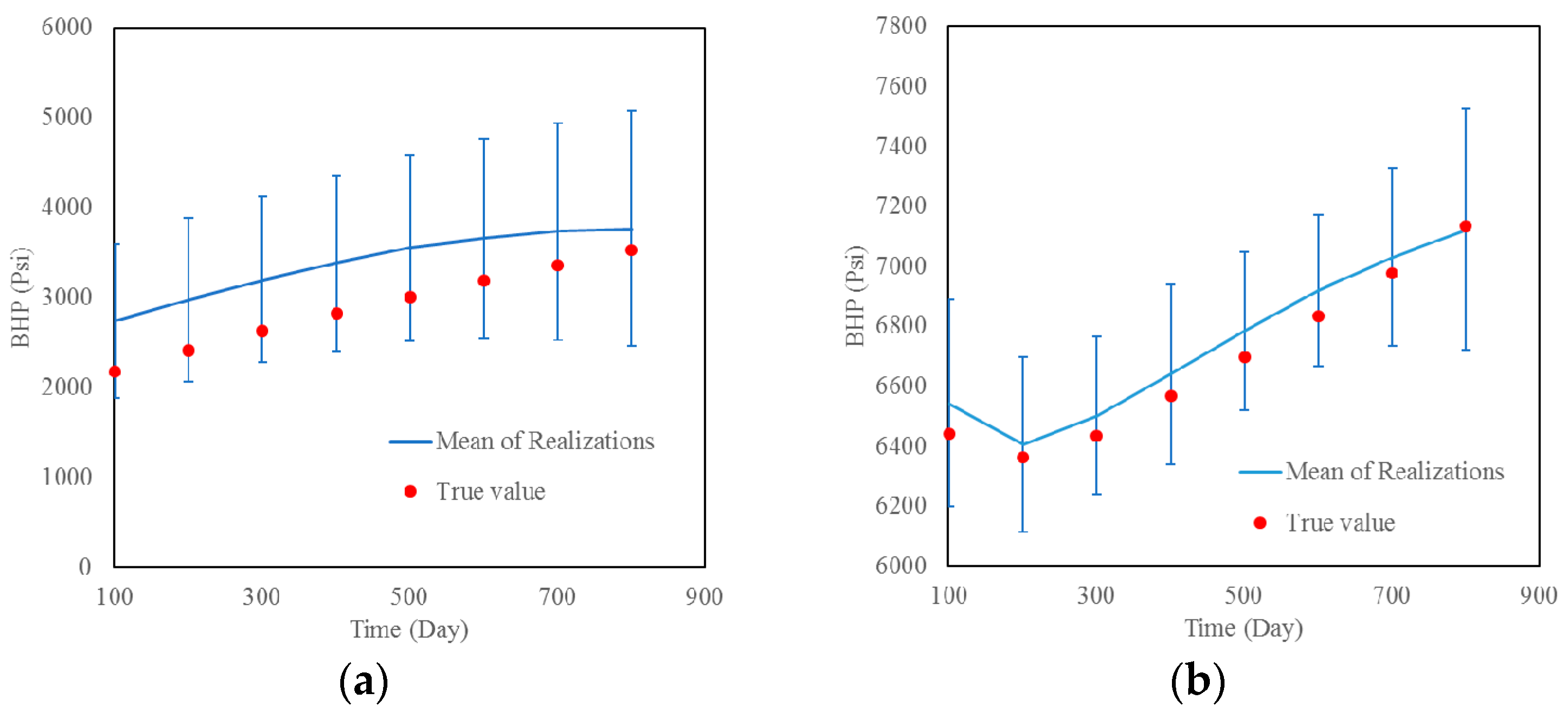
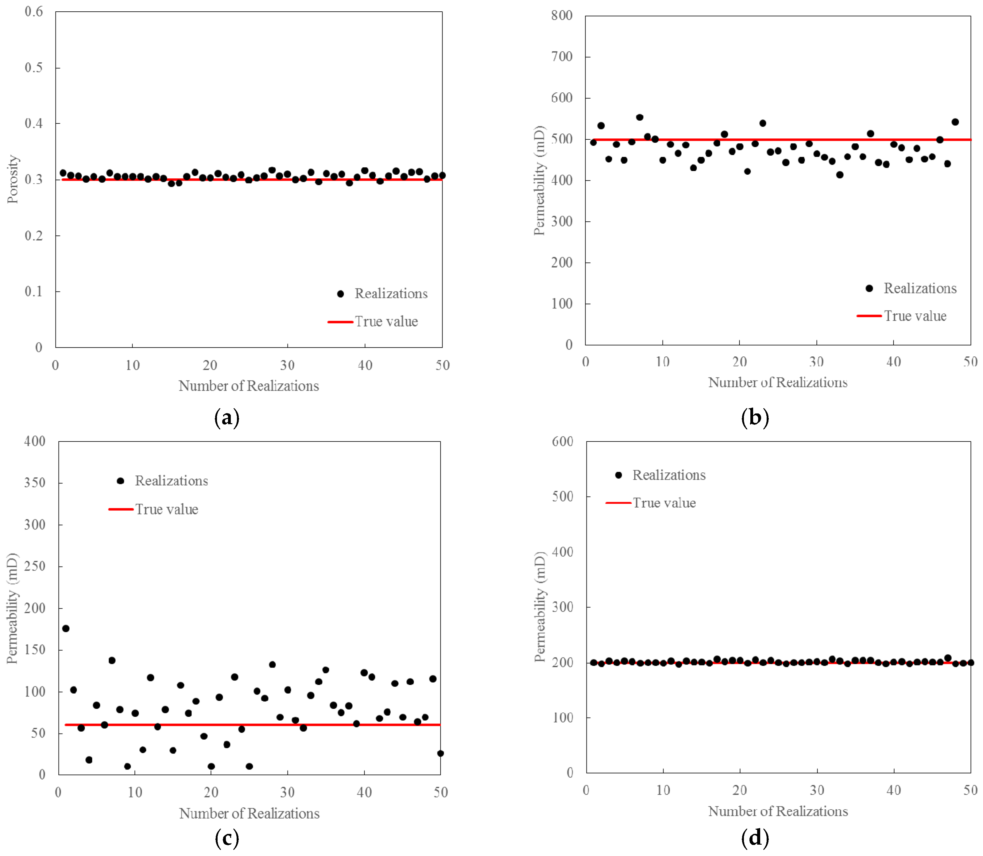
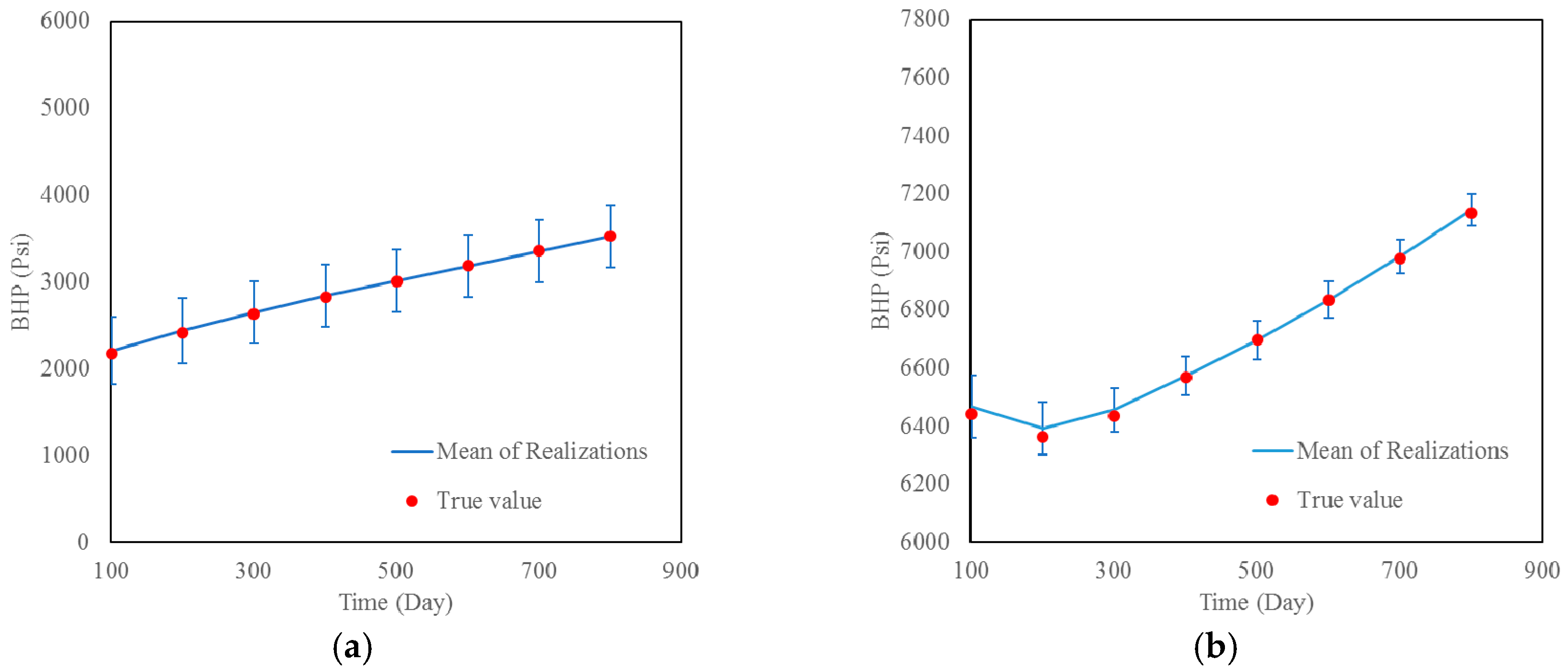
History matching is an important function in GenPack to assist us to take advantage of the observation data. GenPack applies the EnKF method in history matching. The method is validated with a synthetic case. The results show that the prediction accuracy can be greatly improved and the predictive uncertainty can be dramatically reduced after the implementation of history matching.
(5)
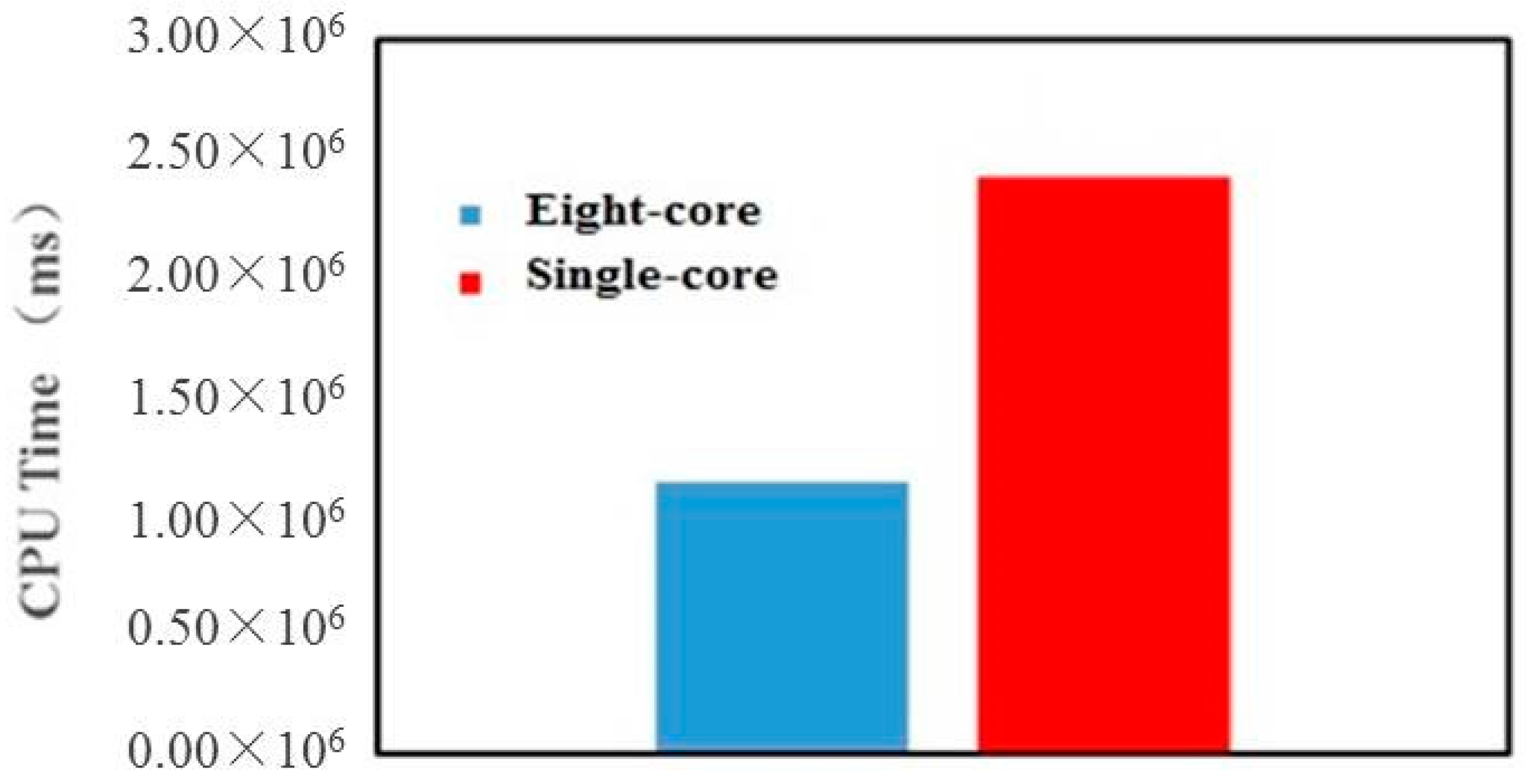
GenPack is a Monte Carlo-based non-intrusive software package ready to be incorporated with any existing simulator in the petroleum engineering field. Due to the independence characteristics when evaluating each realization in the MC process, the efficiency of the stochastic analysis can be further improved with parallel computing when the required computing source is available.

Acknowledgments

This work is funded by the National Natural Science Foundation of China (Grant No. 41402199), National Science and Technology Major Project (Grant No. 2016ZX05037003, 2016ZX05060002), the Science Foundation of China University of Petroleum—Beijing (Grant No. 2462014YJRC038), the independent research funding of State Key Laboratory of Petroleum Resources and Prospecting (Grant No. PRP/indep-4-1409), China Postdoctoral Science Foundation (Grant No. 2016M591353), and the Science Foundation of Sinopec Group (Grant No. P16063).

Author Contributions

Cheng Dai developed the GenPack software package; Liang Xue performed the synthetic tests and wrote the paper; Lei Wang designed the parallel computing.

Conflicts of Interest

The authors declare no conflict of interest

References

  1. Zhang, D. Stochastic Methods for Flow in Porous Media: Coping with Uncertainties; Academic Press: New York, NY, USA, 2001. [Google Scholar]
  2. Xiu, D. Numerical Methods for Stochastic Computations: A Spectral Method Approach; Princeton University Press: Princeton, NJ, USA, 2010. [Google Scholar]
  3. Xiu, D.; Karniadakis, G.E. The Wiener--Askey polynomial chaos for stochastic differential equations. SIAM J. Sci. Comput. 2002, 24, 619–644. [Google Scholar] [CrossRef]
  4. Bakr, A.A.; Gelhar, L.W.; Gutjahr, A.L.; Macmillan, J.R. Stochastic analysis of spatial variability in subsurface flows: 1. Comparison of one- and three-dimensional flows. Water Resour. Res. 1978, 14, 263–271. [Google Scholar] [CrossRef]
  5. Gelhar, L.W. Stochastic subsurface hydrology from theory to applications. Water Resour. Res. 1986, 22. [Google Scholar] [CrossRef]
  6. James, A.L.; Oldenburg, C.M. Linear and Monte Carlo uncertainty analysis for subsurface contaminant transport simulation. Water Resour. Res. 1997, 33, 2495–2508. [Google Scholar] [CrossRef]
  7. Kuczera, G.; Parent, E. Monte Carlo assessment of parameter uncertainty in conceptual catchment models: The Metropolis algorithm. J. Hydrol. 1998, 211, 69–85. [Google Scholar] [CrossRef]
  8. Liu, N.; Oliver, D.S. Evaluation of Monte Carlo methods for assessing uncertainty. SPE J. 2003, 8, 188–195. [Google Scholar] [CrossRef]
  9. Xiu, D.; Karniadakis, G.E. Modeling uncertainty in flow simulations via generalized polynomial chaos. J. Comput. Phys. 2003, 187, 137–167. [Google Scholar] [CrossRef]
  10. Li, H.; Zhang, D. Probabilistic collocation method for flow in porous media: Comparisons with other stochastic methods. Water Resour. Res. 2007, 43. [Google Scholar] [CrossRef]
  11. Li, H.; Zhang, D. Efficient and accurate quantification of uncertainty for multiphase flow with the probabilistic collocation method. SPE J. 2009, 14, 665–679. [Google Scholar] [CrossRef]
  12. Romero, C.E.; Carter, J.N. Using genetic algorithms for reservoir characterisation. J. Pet. Sci. Eng. 2001, 31, 113–123. [Google Scholar] [CrossRef]
  13. Dong, Y.; Oliver, D.S. Quantitative use of 4D seismic data for reservoir description. In Proceedings of the SPE Annual Technical Conference and Exhibition, Denver, CO, USA, 5–8 October 2003.
  14. Gao, G.; Reynolds, A.C. An improved implementation of the LBFGS algorithm for automatic history matching. In Proceedings of the SPE Annual Technical Conference and Exhibition, Houston, TX, USA, 26–29 September 2004.
  15. Ballester, P.J.; Carter, J.N. A parallel real-coded genetic algorithm for history matching and its application to a real petroleum reservoir. J. Pet. Sci. Eng. 2007, 59, 157–168. [Google Scholar] [CrossRef]
  16. Chen, Y.; Zhang, D. Data assimilation for transient flow in geologic formations via ensemble Kalman filter. Adv. Water Resour. 2006, 29, 1107–1122. [Google Scholar] [CrossRef]
  17. Oliver, D.S.; Reynolds, A.C.; Liu, N. Inverse Theory for Petroleum Reservoir Characterization and History Matching; University Press: Cambridge, UK, 2008. [Google Scholar]
  18. Liu, G.; Chen, Y.; Zhang, D. Investigation of flow and transport processes at the MADE site using ensemble Kalman filter. Adv. Water Resour. 2008, 31, 975–986. [Google Scholar] [CrossRef]
  19. Aanonsen, S.; Nævdal, G.; Oliver, D.; Reynolds, A.; Vallès, B. The Ensemble Kalman Filter in Reservoir Engineering—A review. SPE J. 2009, 14, 393–412. [Google Scholar] [CrossRef]
  20. Xie, X.; Zhang, D. Data assimilation for distributed hydrological catchment modeling via ensemble Kalman filter. Adv. Water Resour. 2010, 33, 678–690. [Google Scholar] [CrossRef]
  21. Dai, C.; Xue, L.; Zhang, D.; Guadagnini, A. Data-worth analysis through probabilistic collocation-based Ensemble Kalman Filter. J. Hydrol. 2016, 540, 488–503. [Google Scholar] [CrossRef]
  22. Lorentzen, R.J.; Naevdal, G.; Valles, B.; Berg, A.; Grimstad, A.-A. Analysis of the ensemble Kalman filter for estimation of permeability and porosity in reservoir models. In Proceedings of the SPE Annual Technical Conference and Exhibition, San Antonio, TX, USA, 24–27 September 2006.
  23. Gao, G.; Reynolds, A.C. An improved implementation of the LBFGS algorithm for automatic history matching. SPE J. 2006, 11, 5–17. [Google Scholar] [CrossRef]
  24. Gu, Y.; Oliver, D.S. History Matching of the PUNQ-S3 Reservoir Model Using the Ensemble Kalman Filter. SPE J. 2005, 10, 217–224. [Google Scholar] [CrossRef]
  25. Liao, Q.; Zhang, D. Probabilistic collocation method for strongly nonlinear problems: 1. Transform by location. Water Resour. Res. 2013, 49, 7911–7928. [Google Scholar] [CrossRef]
  26. Wiener, N. The Homogeneous Chaos. Am. J. Math. 1938, 60, 897–936. [Google Scholar] [CrossRef]
  27. Ghanem, R.G.; Spanos, P.D. Stochastic Finite Elements: A Spectral Approach; Courier Corporation: Chelmsford, MA, USA, 2003. [Google Scholar]
  28. Li, H.; Sarma, P.; Zhang, D. A Comparative Study of the Probabilistic-Collocation and Experimental-Design Methods for Petroleum-Reservoir Uncertainty Quantification. SPE J. 2011, 16, 429–439. [Google Scholar] [CrossRef]
  29. Ghanem, R. Scales of fluctuation and the propagation of uncertainty in random porous media. Water Resour. Res. 1998, 34, 2123–2136. [Google Scholar] [CrossRef]
  30. Mathelin, L.; Hussaini, M.Y.; Zang, T.A. Stochastic approaches to uncertainty quantification in CFD simulations. Numer. Algorithms 2005, 38, 209–236. [Google Scholar] [CrossRef]
  31. Tatang, M.A.; Pan, W.; Prinn, R.G.; McRae, G.J. An efficient method for parametric uncertainty analysis of numerical geophysical models. J. Geophys. Res. Atmos. 1997, 102, 21925–21932. [Google Scholar] [CrossRef]
  32. Deutsch, C.V.; Journel, A.G. GSLIB: Geostatistical Software Library and User’s Guide, 2nd ed.; Applied Geostatistics Series; Oxford University Press: New York, NY, USA, 1998. [Google Scholar]
Figure 1. The structure of Genpack. KL: Karhunen–Loeve; MCS: Monte Carlo simulation; PCM: Probabilistic collocation method.
Energies 10 00197 g001
Figure 2. The random field generated by KL expansion with 1000 leading terms: (a) histogram of fields; (b) the contour of the field.
Energies 10 00197 g002
Figure 3. The random field generated by KL expansion with 100 leading terms. (a) marginal distribution of fields; (b) the contour of the field.
Energies 10 00197 g003
Figure 4. The log permeability field with a relatively large cell size generated by GenPack.
Energies 10 00197 g004
Figure 5. A random horizontal permeability field in the corner grid system generated by GenPack.
Energies 10 00197 g005
Figure 6. The comparison results of MCS and PCM in the uncertainty analysis of the producer bottom hole pressure (BHP). (a) Mean value; (b) Standard deviation (STD).
Energies 10 00197 g006
Figure 7. The comparison results of MCS and PCM in the uncertainty analysis of injector BHP. (a) Mean value; (b) Standard deviation (STD).
Energies 10 00197 g007
Figure 8. The CPU time of implementing a MCS case in the single-core and eight-core computers.
Energies 10 00197 g008
Figure 9. The parameter values before history matching: (a) Porosity; (b) Permeability in layer 1; (c) Permeability in layer 2; and (d) Permeability in layer 3.
Energies 10 00197 g009
Figure 10. The predictions (mean with the 95% confidence intervals) before history-matching: (a) Producer BHP; (b) Injector BHP.
Energies 10 00197 g010
Figure 11. The parameter values after history matching: (a) Porosity; (b) Permeability in layer 1; (c) Permeability in layer 2; (d) Permeability in layer 3.
Energies 10 00197 g011
Figure 12. The predictions (mean with the 95% confidence intervals) after history-matching: (a) Producer BHP; (b) Injector BHP.
Energies 10 00197 g012
Table 1. The statistical features of uncertain parameters.
ParameterLayerMinMax
Porosity1–30.10.5
Permeability1200 mD750 mD
Permeability230 mD150 mD
Permeability3100 mD500 mD
Table 2. The parameters used in the reference case.
ParametersLayerTrue Value
Porosity1–30.3
Permeability1500 mD
Permeability260 mD
Permeability3200 mD

