Article

Theoretical Analysis for Heat Transfer Optimization in Subcritical Electrothermal Energy Storage Systems

1
Department of Thermal Science and Energy Engineering, University of Science and Technology of China, Hefei 230027, China
2
Quanzhou Institute of Equipment Manufacturing, Haixi Institutes, Chinese Academy of Sciences, Jinjiang 362200, China
*
Author to whom correspondence should be addressed.
Energies 2017, 10(2), 198; https://doi.org/10.3390/en10020198
Submission received: 21 September 2016 / Revised: 17 November 2016 / Accepted: 11 January 2017 / Published: 10 February 2017

Abstract

:
Electrothermal energy storage (ETES) provides bulk electricity storage based on heat pump and heat engine technologies. A subcritical ETES is described in this paper. Based on the extremum principle of entransy dissipation, a geometry model is developed for heat transfer optimization for subcritical ETES. The exergy during the heat transfer process is deduced in terms of entropy production. The geometry model is validated by the extremum principle of entropy production. The theoretical analysis results show that the extremum principle of entransy dissipation is an effective criterion for the optimization, and the optimum heat transfer for different cases with the same mass flux or pressure has been discussed. The optimum heat transfer can be achieved by adjusting the mass flux and pressure of the working fluid. It also reveals that with the increase of mass flux, there is a minimum exergy in the range under consideration, and the exergy decreases with the increase of the pressure.

1. Introduction

Energy storage plays an important role in energy utilization and conversion systems. The different forms of energy that can be stored include mechanical, electrical and thermal energy [1]. Thermal energy storage (TES) has been proven to be a method to improve the flexibility of energy supply systems and to reduce energy consumption [2]. In these systems energy can be stored as a change in internal energy of a material as sensible heat, latent heat and thermochemical or some combination of these, and it already has been widely applied in thermal solar power plants [3], water heater storage [4], solar latent heat storage unit [5,6] and so on. It is also found that TES has been employed to contribute electrothermal energy storage (ETES), which is a type of bulk electricity storage technology to balance power demand and supply. ETES is based on heat pump and heat engine technologies [7]. It uses a heat pump system to transfer electrical energy combined with TES to convert electrical energy into thermal energy in the off peak electrical output periods; during periods of peak power consumption in the electric network the stored energy is then converted back into electrical energy using a heat engine. Compared with pumped hydroelectric storage and compressed air energy storage, the advantage of ETES is that it is not restricted by geographical constraints and covers small to large capacities [8,9].
Some researchers have proposed a combination of a heat pump and a heat engine to store energy [10,11], and some studies have been carried out on the optimizations for ETES. Peterson [12] and Henchoz et al. [13] noted the effectiveness of sub-ambient temperature ETES. White et al. [14] investigated the thermodynamic aspects of a pumped thermal electricity storage system, and showed that highly efficient compression and expansion processes are clearly required to obtain a satisfactory cycle efficiency. Meanwhile, the transcritical CO2 Rankine cycle has been proposed to replace the Rankine cycle as the thermodynamic cycle, which is allowing for higher roundtrip efficiency in heat exchange process [15]. Kim et al. [16] proposed a novel isothermal ETES with transcritical CO2 cycles, which shows higher roundtrip efficiency because of a lower back work ratio than in the isentropic case. Furthermore, the heat transfer of ETES plays an important role in the system performance [17]. Morandin [18,19] used pinch analysis tools to optimize various forms of transcritical CO2 cycle based ETES. They showed that the thermal energy available from the heat pump condenser at high temperatures can be stored and further used in a more efficient way, and the heat transfer feasibility must also be required in the optimization. Baik et al. [20] showed that an optimum temperature exists in the low-temperature hot storage tank for maximizing the roundtrip efficiency. Desrues [8] presented a thermal energy storage process for large scale electric applications based on a high temperature heat pump cycle and a heat engine cycle. The increase of the heat exchange is identified as a key factor to approach the theoretical storage efficiency.
Many studies focus on ETES utilizing transcritical CO2 cycle, however, the expander or turbine for transcritical CO2 cycles is complicated and expensive in practice. On the other hand, high temperature thermal storage may result in large heat losses. Therefore, in this study, a subcritical ETES is presented and a geometry model is developed for the optimization of the heat transfer process. The optimal parameters (mass flux, pressure) are theoretically investigated.

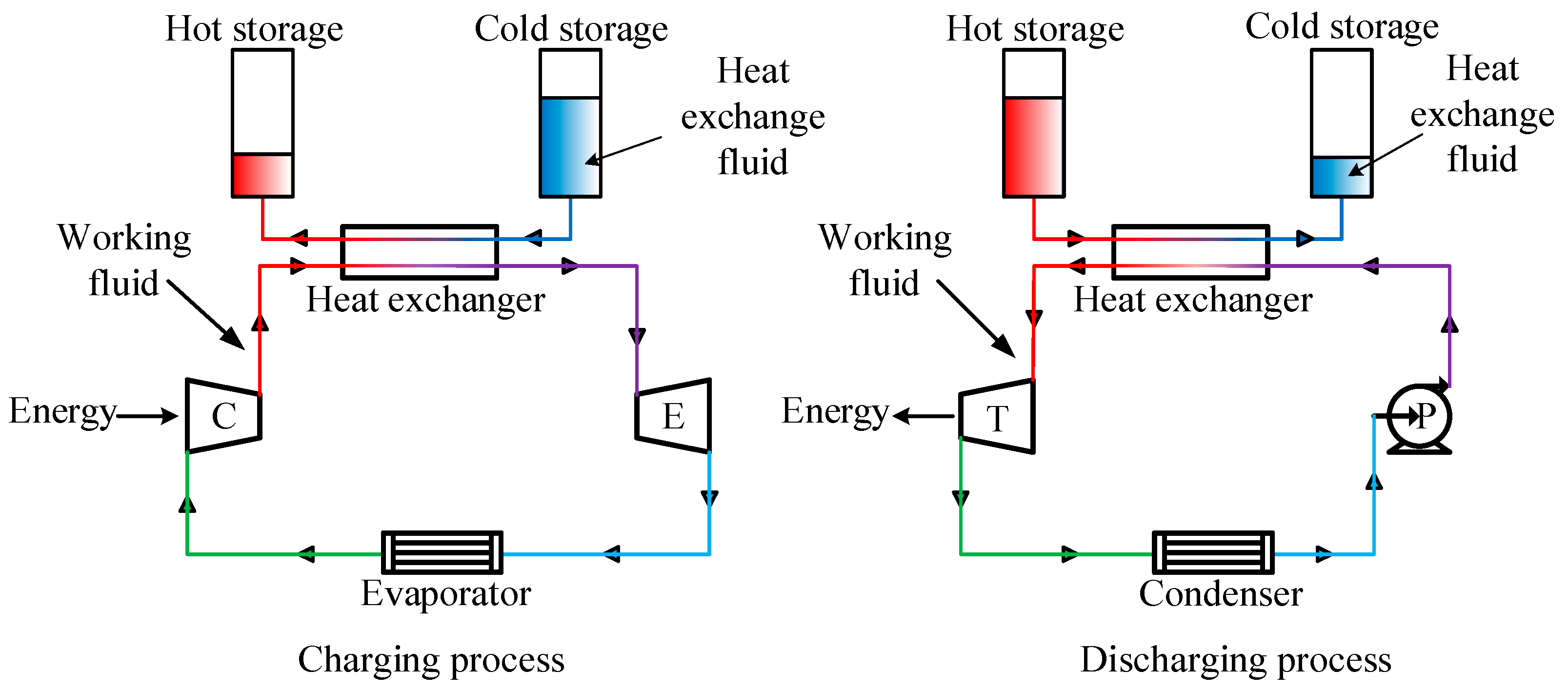
2. Theoretical Analysis

As for the theoretical analysis, it is well known that the entropy production of a thermal system at steady-state should be the minimum, so many researchers have developed the concept of entropy production to deal with heat transfer optimization. Bejan [21] proposed the entropy production expressions to optimize the geometry of heat transfer tubes and find the parameters to achieve the optimum heat transfer. Johannesse [22] presented a theoretical proof that the entropy production due to heat exchange in a heat exchanger is minimum when the local entropy production is constant in all parts of the system. Balkan [23] presented a more realistic application of the entropy minimization principle Equipartition of Entropy production (EoEP). It dictates uniform local entropy productions along the heat exchanger in order to minimize the total entropy production rate due only to heat transfer. In recent years, a new physical quantity has been identified by Guo et al. [24] which is a basis for optimizing heat transfer process in terms of the analogy between heat and electrical conduction. Guo et al. [25] established a principle Equipartition of Entransy Dissipation (EoED) for heat exchanger design, which says that for a heat exchanger design with given heat duty and heat transfer area, the total entransy dissipation rate reaches the minimum value when the local entransy dissipation rate is uniformly distributed along the heat exchanger, which means the optimum heat transfer can be achieved with the minimum entransy dissipation. However, as far as we know, few research works have optimized the heat transfer for ETES by the principles EoEP and EoED. And the purpose of this article is to make an optimization by these two principles.
Figure 1 shows a schematic diagram of the ETES. For a subcritical cycle, there are three zones during heat transfer process for working fluid: liquid zone, phase change zone and vapor zone. To simplify the model, some assumptions are made:
  • The charging process is fixed, and the total heat exchange capacity of the charging and discharging process are equivalent, and the heat exchange is mainly based on the latent heat exchange;
  • The variations of isobaric specific heat and latent heat with minor change of pressure can be ignored, thus the isobaric specific heat and latent heat are assumed to be constants;
  • The pinch point temperature difference is assumed to be zero; the heat loss of the heat exchange process is taken no account.
According to the theory of Guo et al. [24], the optimization of a heat conduction process minimizes the equivalent thermal resistance for the constraints. The minimum entransy dissipation implies the minimum thermal resistance for a given boundary heat flux, while the maximum entransy dissipation implies the minimum thermal resistance for a given set of boundary temperature. The extremum principle of entransy dissipation can also be applied to the optimization of heat convection processes. In our model, the total heat exchange capacity and area of the heat exchanger are fixed, that is to say the heat is exchanged by a given boundary heat flux, thus the entransy dissipation must achieve the minimum value to obtain the optimum heat transfer. Because the specific heat capacity is assumed constant for a given working fluid, the entransy dissipation can be simplified by calculating the area of a quantity of triangles.
For the charging process, the entransy dissipation can be presented as:
E h , c h = E h , c h E h , h x = 1 2 H 1 H 2 [ T c h ( H , p ) T h x ( H , p ) ] d H = 1 2 ( S a + S b )
As shown in Figure 2, the heat exchange line changes from solid line to any dotted line, the entransy dissipation will increase, it is because that h a is higher than h b obviously due to the large latent heat. Thus, the entransy dissipation of the charging process reaches the minimum when the heat exchange line pass through points ( H 1 ,   T o ) and ( H c 1 ,   T 1 ) . The slope of the heat exchange line can be expressed as following:
k = T 1 T o H c 1 H 1 = T 1 T o x
Similarly, the entransy dissipation of the discharging process is:
E h , d s = E h , h x E h , d s = 1 2 H 1 H 2 [ T h x ( H , p ) T d s ( H , p ) ] d H = 1 2 ( A 1 + A 2 )
where A 1 and A 2 are the areas of S 1 , S 2 in Figure 3.
Therefore the heat exchange line can be expressed as:
k ( H H c 1 ) = T T 1
For the triangle S 1 shown in Figure 3, the height h 1 and base d 1 of S 1 can be expressed by the following equations due to the ( H c 2 , T 2 ) is on the heat exchange line, therefore:
h 1 = H c 2 H 1 = T 2 T 1 k + H c 1 H 1 = x Δ T k = α
where x is the enthalpy difference between the end of the charging process and the beginning of the phase change stage. Similarly α is the enthalpy difference between the beginnings of the discharging process and the phase change stage:
d 1 = T o T i , b
with:
( T 2 T i , b ) = H c 2 H 1 = α
k ( H 1 H c 1 ) = T o T 1
Thus:
d 1 = k α + α m c 1
A 1 = 1 2 ( α m c 1 k α ) α = 1 2 ( α 2 m c 1 k α 2 )
As for S 2 , it can be calculated by S 21 + S 22 obviously, where the height and base of S 21 can be deduced by the equations below:
h 21 = T o , b T 2
d 21 = m h m
With the slope equation of the vapor stage:
k v a p = 1 m c 2 = T o , b T 2 h 2 ( h c 2 + m h m )
where:
y + Δ T k = β
Thus:
h 21 = T o , b T 2 = β m h m m c 2
A 21 = 1 2 m h m × β m h m m c 2 = 1 2 β h m m h m 2 c 2
Similarly, the height and base of S 22 can also be expressed:
h 22 = H 2 H c 2 = H 2 T 2 T 1 k H c 1 = β
d 22 = T x T o , b
with:
T x = k y + T 1
And the T o , b can be deduced by Equation (15), therefore:
A 22 = 1 2 β × ( k β β m h m m c 2 ) = 1 2 ( k β 2 β 2 β m h m m c 2 )
Base on the equations above, the area of S 2 ( A 2 ) and the whole area between heat exchange line and discharging process line ( A ) can be obtained as:
A = A 1 + A 2 = A 1 + A 21 + A 22 = 1 2 ( α 2 m c 1 k α 2 + k β 2 ( β m h m ) 2 m c 2 )
where A corresponds to the entransy dissipation of the discharging process E h :
E h = 1 2 H 1 H 2 [ T h x ( H , p ) T d s ( H , p ) ] d H = 1 2 A = 1 4 ( α 2 m c 1 k α 2 + k β 2 ( β m h m ) 2 m c 2 )

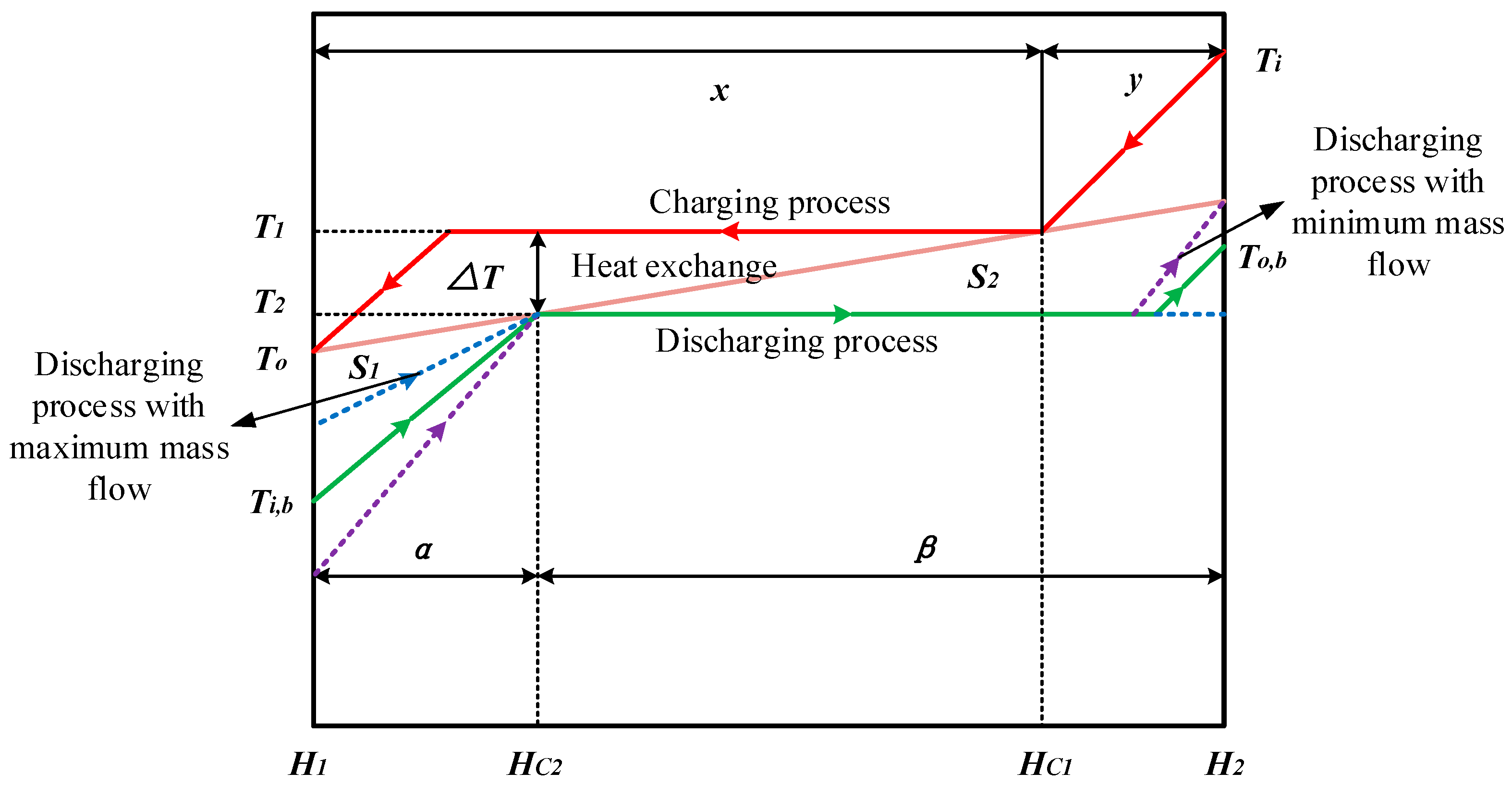
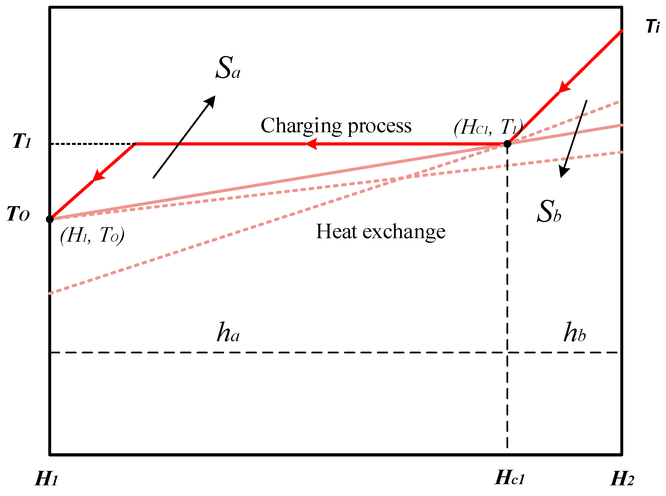
2.1. Optimum Heat Transfer at Different Mass Fluxes

The minimum entransy dissipation has been demonstrated to represent the optimum heat transfer in this model. In the discharging process, to study the influence of mass flux on the heat transfer process, the pressure is assumed constant. Thus other thermodynamic properties are fixed under the same pressure, the mass flux is the only variable parameter. The range of the mass flux has been dominated by the assumptions of the heat exchange model in this study. The minimum and maximum mass flux are limited by the outlet temperature of the discharging process shown in Figure 4.
The outlet temperature of the discharging process at the minimum mass flux is equal to the outlet temperature of the heat exchange fluid. Therefore:
1 m m i n c 2 = k y + T 1 T 2 h 2 ( h c 2 + m m i n h m )
m m i n = β k β c 2 + h m
E h ( m m i n ) = A m m i n = 1 2 ( α 2 h m β c 1 + α 2 k c 2 c 1 k α 2 + k β 2 h m k β c 2 + h m )
As for the maximum mass flux, the outlet temperature of the discharging process is equal to the phase change temperature of the discharging process, with:
m m a x h m + H c 2 = H 2
Thus:
m m a x = H 2 H c 2 h m = β h m
E h ( m m a x ) = A m m a x = 1 2 ( α 2 h m β c 1 k α 2 + k β 2 )
Therefore the range of mass flux is ( β k β c 2 + h m , β h m ) .
The relative influence of mass flux on the entransy dissipation can be expressed by the equation:
( E h m , p ) ( m ) = 1 4 ( α 2 m 2 c 1 m 2 h m 2 β 2 m 2 c 2 )
The extremum mass flux of the maximum entransy dissipation is:
m e x = c 1 β 2 c 2 α 2 c 1 h m 2 < β h m
To calculate the minimum entransy dissipation, the entransy dissipations at the minimum and maximum mass flux are compared:
Δ A = A m m i n A m m a x = 1 2 ( α 2 k c 2 c 1 k 2 β 3 c 2 k β c 2 + h m )
Thus:
When α 2 β 2 < k β c 1 k β c 2 + h m , Δ A < 0 :
E h m i n = 1 2 A m i n = 1 2 A m m i n = 1 4 ( α 2 h m β c 1 + α 2 k c 2 c 1 k α 2 + k β 2 k 2 β 3 c 2 k β c 2 + h m )
Thus:
m o p t = m m i n = β k β c 2 + h m
When α 2 β 2 = k β c 1 k β c 2 + h m , Δ A = 0 :
E h m i n = 1 2 A m m i n = 1 2 A m m a x = 1 4 ( α 2 h m β c 1 k α 2 + k β 2 )
Thus:
m o p t = m m i n   or   m m a x
When α 2 β 2 > k β c 1 k β c 2 + h m , Δ A > 0 :
E h m i n = 1 2 A m i n = 1 2 A m m a x = 1 4 ( α 2 h m β c 1 k α 2 + k β 2 )
Thus:
m o p t = m m a x = β h m

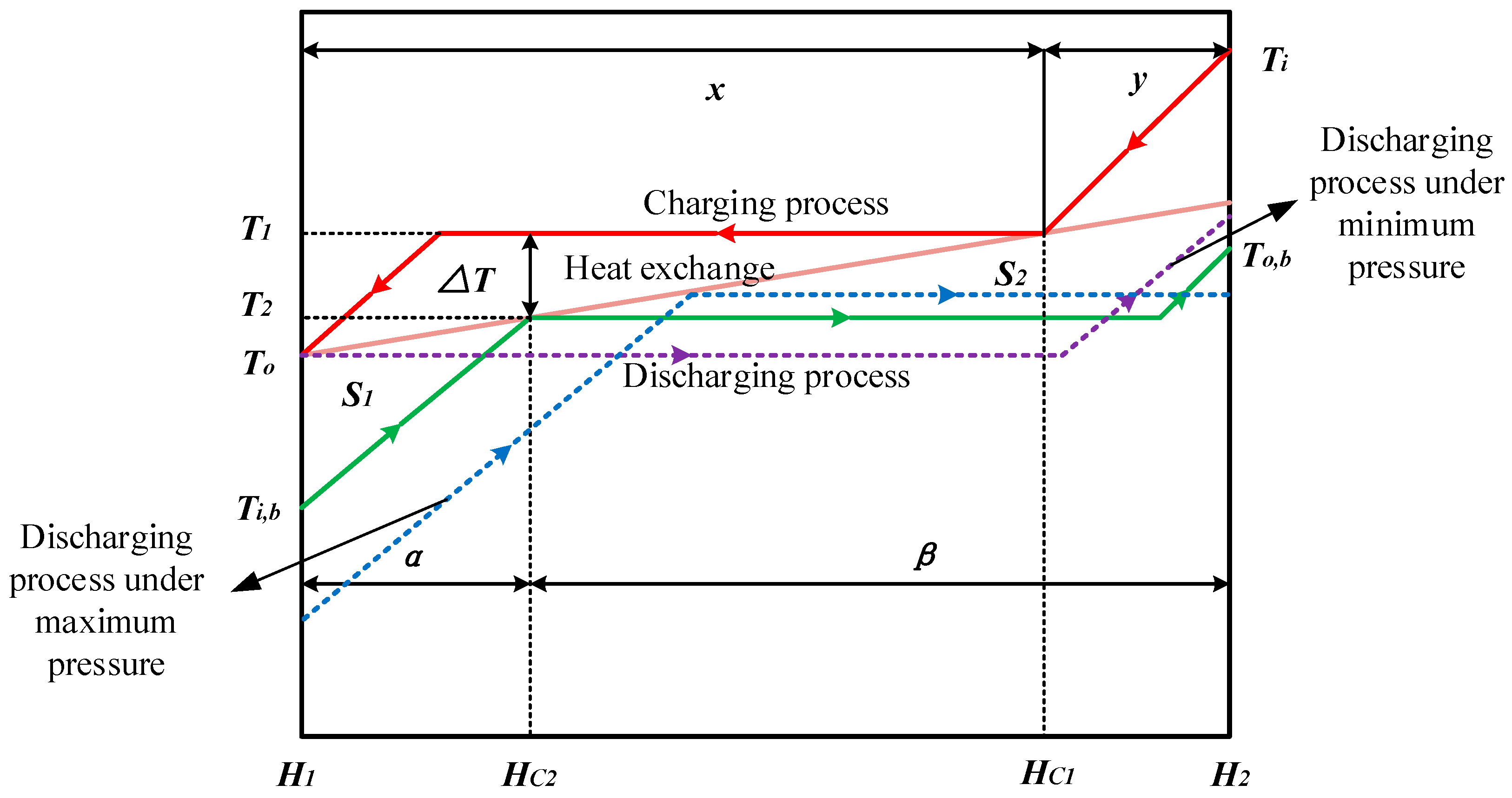
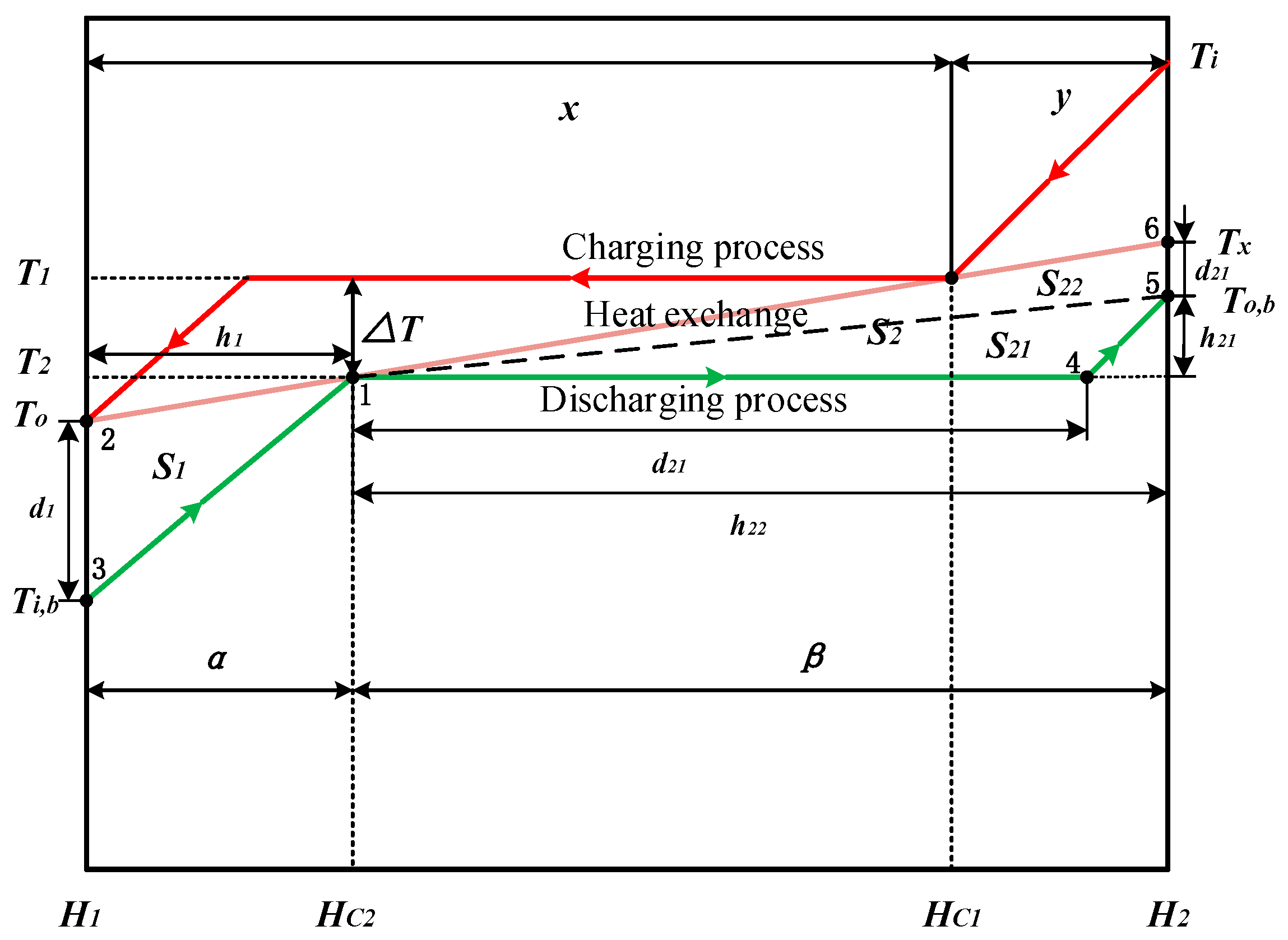
2.2. Optimum Heat Transfer under Different Pressures

Similarly, to present the influence of pressure on the entransy dissipation, is equivalent to assuming that the mass flux is fixed in the discharging process. As we all know, though the latent heat, specific heat and phase change temperature are affected by pressure in the discharging process, the latent heat and specific heat are not taken into account because of the minor changes (compared with the variation of phase change temperature) under various pressure conditions. Therefore, the relative influence of the pressure simply performed as the phase change temperature difference between the charging and discharging process, as shown in Figure 5, the maximum (or minimum) pressure corresponds to the minimum (or maximum) temperature difference:
( E h m , p ) ( Δ T ) = 1 2 ( 2 α α m c 1 2 k α α + 2 k β β 2 β β 2 m h m β m c 2 ) = k m c 1 c 2 ( α + β ) + c 1 m h m ( c 2 α + c 1 β ) k m c 1 c 2
Δ T e x = k c 2 x ( k m c 1 1 ) + k c 1 y ( k m c 2 1 ) + k c 1 m h m c 1 c 2
With:
k c 2 x ( k m c 1 1 ) =   k c 2 ( k m c 1 x x ) = k c 2 m h m
Δ T e x = k m h m k y   c 1 ( 1 k m c 2 ) c 1 c 2
Based on the assumptions about the heat exchange model mentioned above, the phase change temperature difference is limited by the inlet and outlet temperature of the discharging process. The outlet temperature of the discharging process with the minimum phase change temperature difference is equal to the phase change temperature of the discharging process. Then:
β Δ T m i n = m h m = h 2 h c 2 = y + Δ T m i n k
Thus:
Δ T m i n =   k m h m k y
Similarly, the inlet temperature of the discharging process with the maximum phase change temperature difference is equal to the phase change temperature of discharging process, that is to say:
β Δ T m a x = x + y
then:
Δ T m a x = k x
Therefore the range of the phase change temperature difference between the charging and discharging process is ( k m h m k y , k x ) as shown in Figure 5.
As we all know, the slope of the heat exchange line is smaller than the slope of the liquid or vapor stage, which means:
k < 1 m c 1   and   k < 1 m c 2
When c 1 > c 2 :
c 1 c 2 c 1 < 1 k m c 2
1 <     c 1 ( 1 k m c 2 ) c 1 c 2
Δ T e x < Δ T m i n
The entransy dissipation is a monotonous decreasing function of the phase change temperature difference which corresponds to a monotonous increasing function of pressure. It ensures that the entransy dissipation is the minimum with the maximum phase change temperature difference.
When c 1 < c 2 :
c 1 ( 1 k m c 2 ) c 1 c 2 < 0
Δ T e x > Δ T m i n
According to the assumption mentioned above, the sensible heat exchange in liquid and vapor stages are too low, which means they are about equivalent.
m h m + y x
Δ T e x = k m h m k y   c 1 ( 1 k m c 2 ) c 1 c 2 = k ( m h m + y   c 1 ( 1 k m c 2 ) c 2 c 1 )
while:
c 1 ( 1 k m c 2 ) c 2 c 1 < 1
Δ T e x < Δ T m a x
Δ T e x is in the range of the phase change temperature difference between the charging and discharging process. The minimum entransy dissipation can be obtained with the Δ T e x which corresponds to the optimum pressure.
When:
c 1 ( 1 k m c 2 ) c 2 c 1 > 1
then:
Δ T e x > Δ T m a x
The entransy dissipation is also a monotonous decreasing function of the phase change temperature difference. It means the minimum entransy dissipation is obtained at the maximum phase change temperature difference which corresponds to the minimum pressure.
Therefore:
When c 1 > c 2 or c 1 < c 2 , c 1 ( 1 k m c 2 ) c 2 c 1 > 1 :
E h m i n = 1 2 A m i n = 1 2 A Δ T m a x = 1 2 A p m i n
When c 1 < c 2 , c 1 ( 1 k m c 2 ) c 2 c 1 < 1
E h m i n = 1 2 A m i n = 1 2 A Δ T e x
Based on above analyses, it can be known that the optimum heat transfer can be presented by adjusting the mass flux or pressure respectively at a given pressure or mass flux. The main object of this work is to find out the optimum parameters. The significance of entransy dissipation has been researched in previous published papers, and the optimum parameters have certainly been obtained with these theories. On the other hand, this study will also present the minimum entropy production analysis to demonstrate the results shown above.

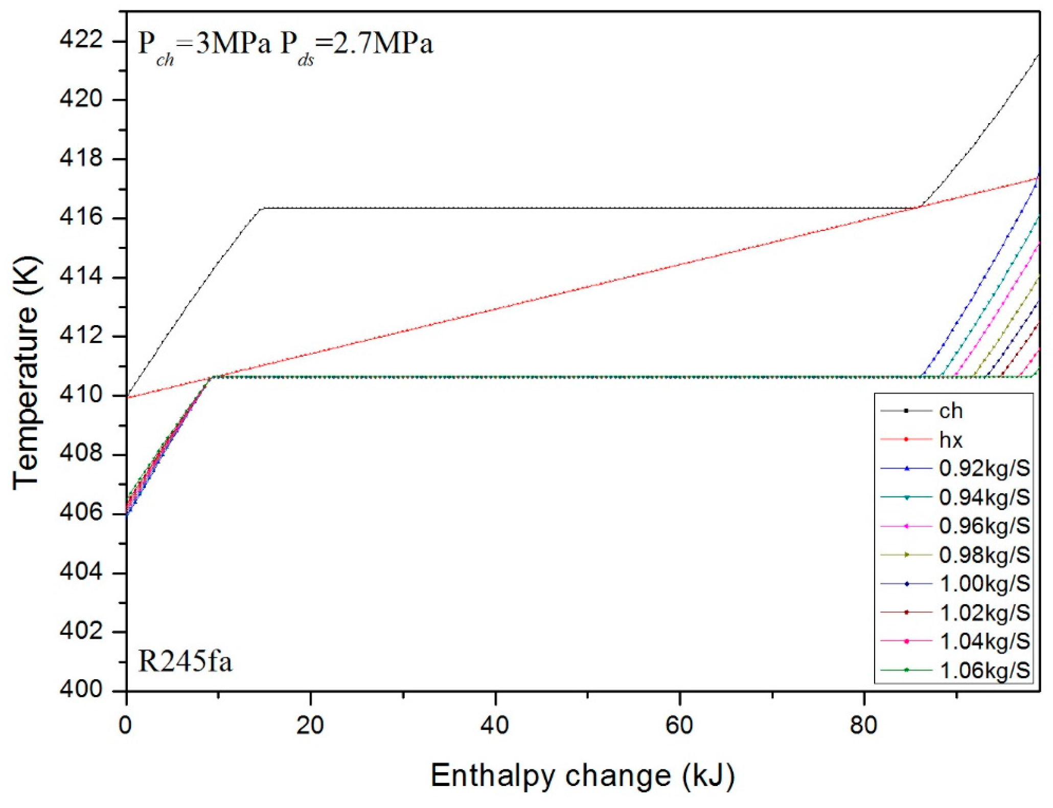
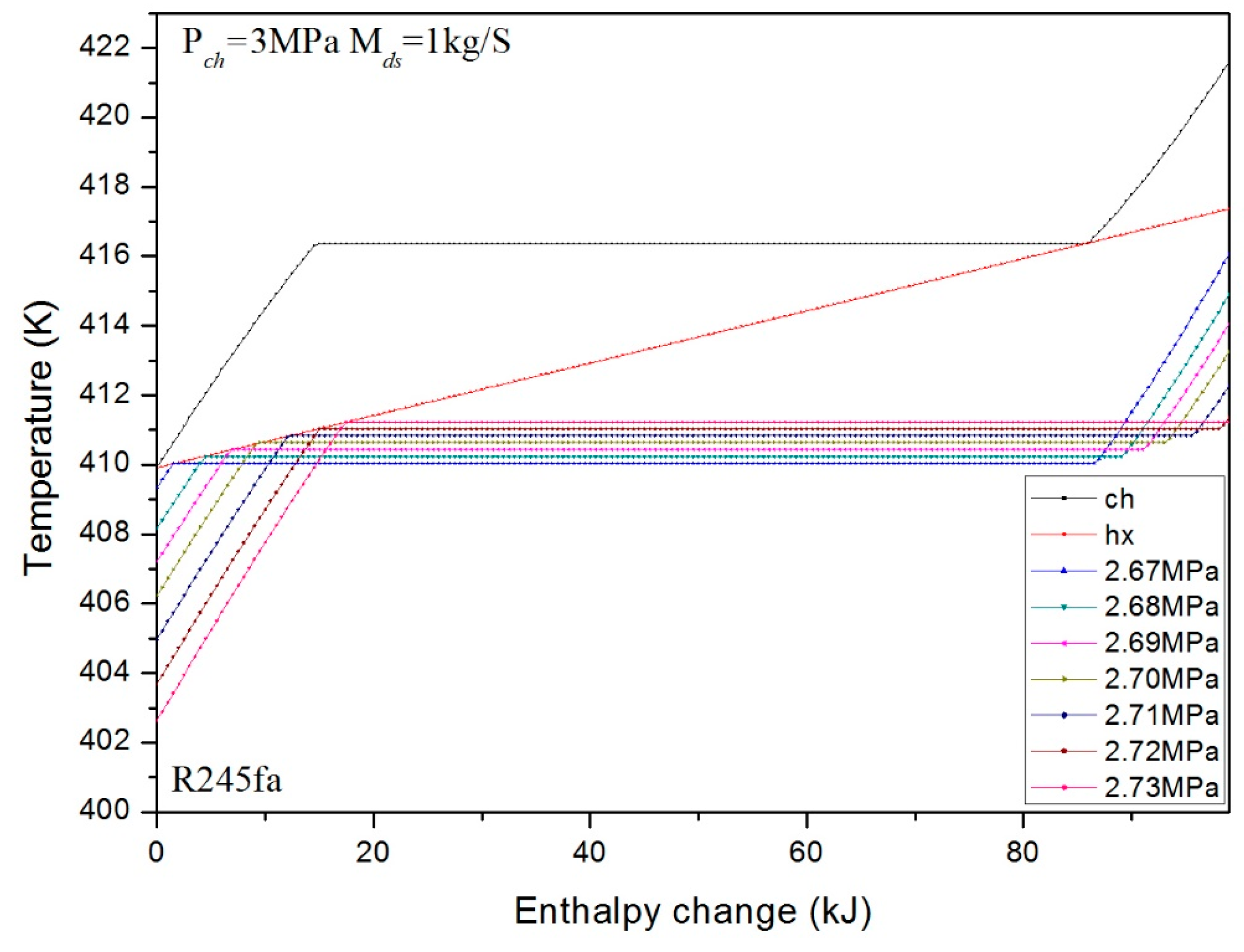
3. Numerical Confirmation of the Optimum Heat Transfer

In order to check the validation of the presented model, a numerical confirmation is carried out for the various mass fluxes and pressures respectively. R245fa is employed for the working fluid using the thermodynamic data from REFPROP 9.0. Figure 6 and Figure 7 show the variation of temperature with the enthalpy change. Figure 6 displays the variation at various mass fluxes under the fixed pressure. It can be found that the outlet temperature of the discharging process decreases with the increasing mass flux. Conversely, the inlet temperature of the discharging process increases. The increasing mass flux causes the enthalpy change of phase change stage more and the slopes of the liquid and vapor stage (shown in the Equation (13)) smaller, resulting in the inlet and outlet temperature changes. Figure 7 displays the variation of temperature under various pressures at the same mass flux. It can be seen that the phase change temperature increases with the increase of pressure. However, as for other thermodynamics properties (isobaric specific heat, latent heat), there are not significant variations, therefore, the inlet temperature increases and outlet temperature decreases as Figure 6 and Figure 7 show.
According to the extremum principle of entropy production, the object of thermodynamic optimization is to minimize the total entropy production. The minimum entropy production corresponds to the maximum exergy. As a consequence, the exergy analysis can be employed for numerical confirmation in this study. The exergy is determined by the temperature and thermodynamic data of the R245fa in the discharging process, which can be calculated by an equation, the exergy of a heat source with limited capacity can be written as:
E u Q = 1 2 ( 1 T 0 T ) d Q = Q 12 T 0 Δ S 12
In the model established previously, the entropy production of the discharging process can be obtained as:
Δ S 12 = m ( c 1 ln T 2 T i , b + h m , 2 T 2 + c 2 ln T o , b T 2 )
The variations of exergy with various mass fluxes and pressures are shown in Figure 8 and Figure 9. The range of the mass flux in this calculation case is (0.92, 1.07) kg / s , it can be found that the exergy decreases firstly, and then increases with increasing mass flux under the same pressure. This means there is a critical point of the minimum exergy just like the m e x deduced by the previous theoretical analysis. The value of m e x is calculated for this case, which is 1.058 kg / s . It is accordingly shown at around m = 1.06   kg / s in Figure 8. On the other hand, the exergy attain the maximum value at the minimum mass flux in the numerical analysis, which means the optimum heat transfer can be obtained at the minimum mass flux. And in this case, α 2 β 2 < k β c 1 k β c 2 + h m is satisfied, that is to say the optimum heat transfer occur at the minimum mass flux demonstrated in the theoretical part. The difference between theoretical analysis and numerical analysis can be performed indirectly via a comparison of the different values of m e x . In this case, the difference is around 0.19%. As a consequence, the optimum heat transfer (minimum eantransy dissipation) at different mass flux of theoretical analysis and the actual optimum heat transfer have achieved a good agreement.
Figure 9 shows the variation of the exergy with pressure at a fixed mass flux of 1   kg / s . In this case, the condition of c 1 < c 2 ,   c 1 ( 1 k m c 2 ) c 2 c 1 > 1 is satisfied. The entransy dissipation is a monotonous increasing function of pressure. The exergy decreases with the increase of pressure in the range of the variable pressure, the maximum exergy is at the minimum pressure which corresponds to the minimum entransy dissipation.

4. Conclusions

The main parameters, mass flux and pressure of working fluid, can affect the roundtrip efficiency of subcritical ETES via heat transfer process. A geometry model based on the entransy dissipation theory is developed to simplify the theoretical analysis and validated by the minimum entropy production principle. The following conclusions can be reached from theoretical analysis of the heat transfer process of subcritical ETES:
  • For the different mass fluxes under fixed pressure, the mass fluxes to achieve the optimum heat transfer are different for different cases. The optimum mass flux is effected mainly by the latent heats of the charging and discharging processes. However, it is confirmed that the optimum mass flux appears at the minimum or maximum allowed value under the same pressure.
  • Similarly, for the different pressures at fixed mass flux, the optimum pressure is effected mainly by the specific heat capacities of the liquid or vapor stages. The optimum heat transfer can be obtained under the minimum pressure with c 1 > c 2   or     c 1 ( 1 k m c 2 ) c 2 c 1 > 1 . We found the reason for this is the entransy dissipation is a monotonous decreasing function for this situation. However, for any other cases, there is an optimum pressure which depends on the extreme phase change temperature difference between charging and discharging processes.
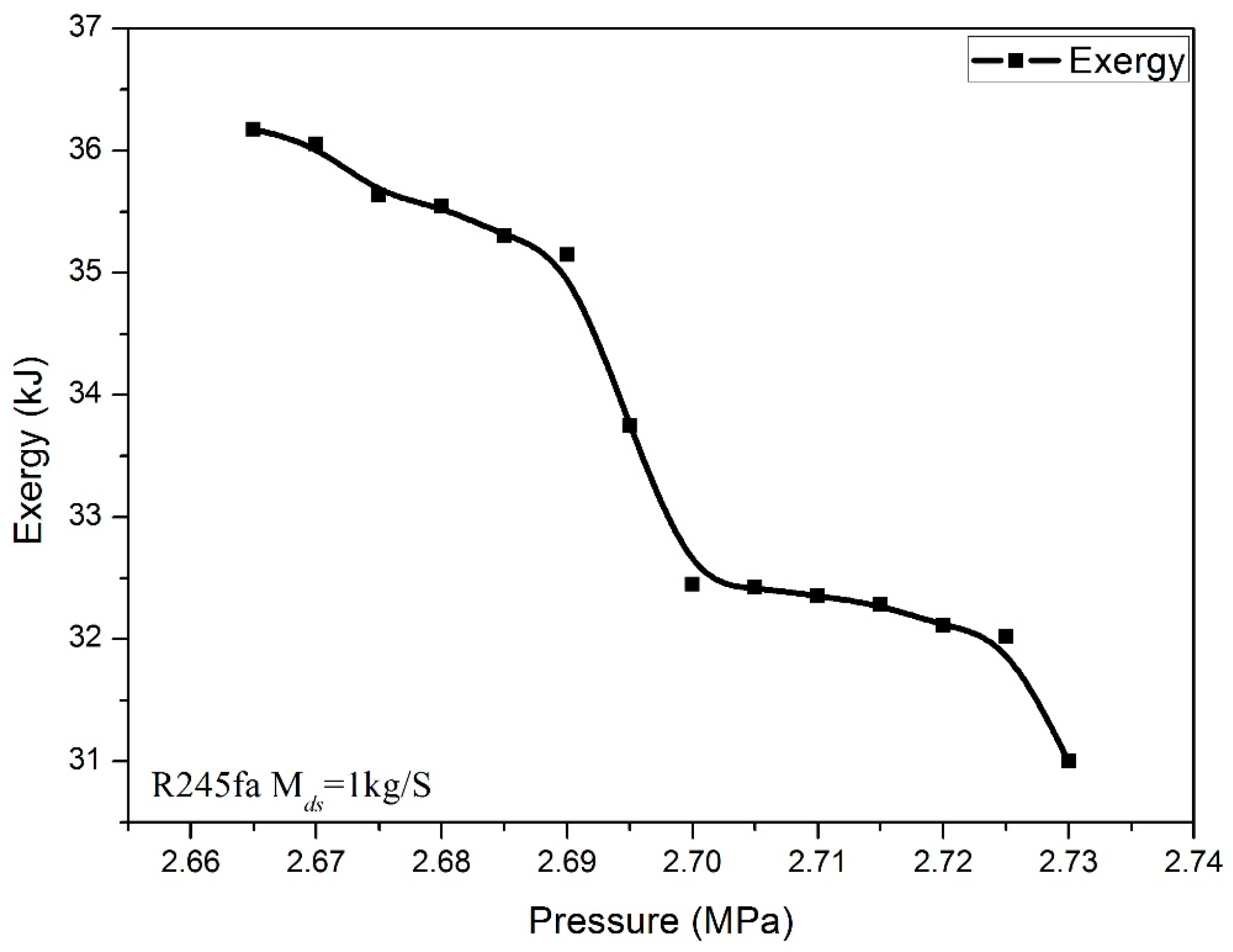
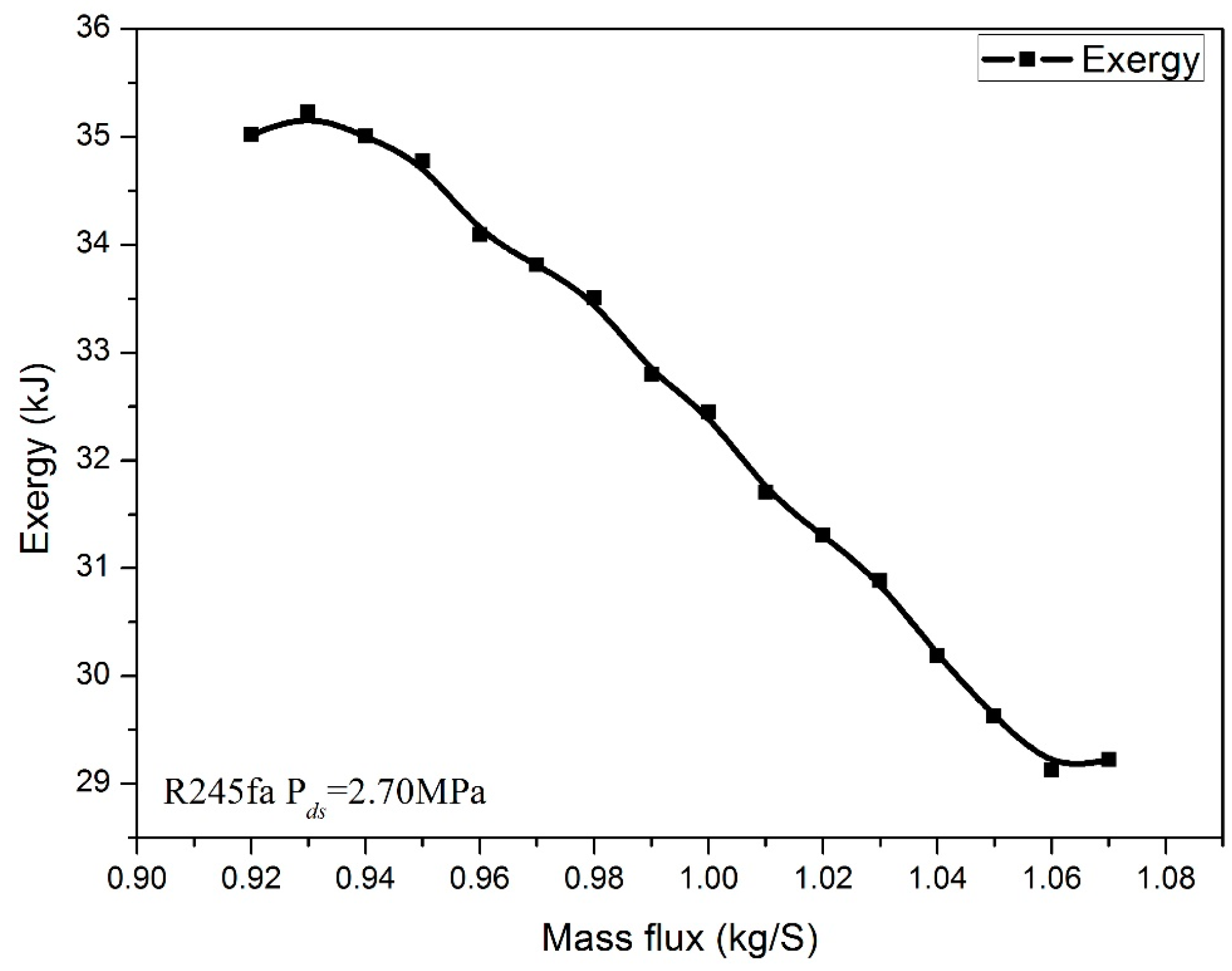
  • In order to demonstrate the validation of the model, the maximum exergy analysis based on the minimum entropy production principle has been carried out. The data of the numerical confirmation is compared with the result proposed by theoretical analysis. There is minor difference (around 0.19% in this study) between the variations of the exergy and entransy dissipation of R245fa.
In summary, to optimize the heat transfer of the ETES system, it is efficient to optimize the mass flux or pressure of the discharging process respectively. The theoretical analysis is proven to be an efficient method to approach the optimum parameters in the ETES.

Acknowledgments

This work was supported by the National Natural Science Foundation of China [grant number 51576187].

Author Contributions

Peng Hu and Gao-Wei Zhang conceived and designed the study. Peng Hu, Gao-Wei Zhang and Long-Xiang Chen performed the experiments. Gao-Wei Zhang and Long-Xiang Chen wrote the paper. Peng Hu and Ming-Hou Liu reviewed and edited the manuscript. All authors read and approved the manuscript.

Conflicts of Interest

We declare that we do not have any commercial or associative interest that represents a conflict of interest in connection with the work submitted.

Abbreviations

A Area
A 1 Area of the triangle S 1
A 21 Area of the triangle S 21
A 22 Area of the triangle S 22
c 1 Liquid isobaric specific heat
c 2 Vapor isobaric specific heat
d 1 Base of the triangle S 1
d 21 Base of the triangle S 21
d 22 Base of the triangle S 22
E h Entransy
E h Entransy dissipation
E u Q Exergy
H Enthalpy
H 1 Enthalpy of the beginning
H 2 Enthalpy of the end
H c 1 Enthalpy of the phase change end in the charging process
H c 2 Enthalpy of the phase change beginning in the discharging process
h m Latent heat
h 1 Height of the triangle S 1
h 21 Height of the triangle S 21
h 22 Height of the triangle S 22
k Slope of the heat exchange line
k v a p Slope of the vapor stage in the discharging process
m Mass flux
p Pressure
S 1 Δ123
S 21 Δ145
S 22 Δ156
T Temperature
T 1 Phase change temperature of the charging process
T 2 Phase change temperature of the discharging process
T i Inlet temperature of the charging process
T o Outlet temperature of the charging process
T i , b Inlet temperature of the discharging process
T o , b Outlet temperature of the discharging process
T 0 Environment temperature
T x Outlet temperature of the heat exchange fluid
Q 12 Heat change
x Enthalpy difference between the end and the phase change beginning of the charging process
y Enthalpy difference between the beginning and the phase change beginning of the charging process
Δ S The area difference between the process with the minimum and maximum mass flux
Δ S 12 Entropy production
Δ T Phase change temperature difference between charging and discharging process
Greek Symbols
α Enthalpy difference between the beginning and the phase change beginning of the discharging process
β Enthalpy difference between the phase change beginning and the end of the charging process
ε Effect degree
φ Thermodynamic properties
Subscripts
e x Extreme value
c h Charging process
h x Heat exchange
d s Discharging process
m i n Minimum
m a x Maximum

References

  1. Khartchenko, N.V. Advanced Energy Systems; Institute of Energy Engineering & Technology University: Berlin, Germany, 1997. [Google Scholar]
  2. Hyman, L. Sustainable Thermal Storage Systems Planning Design and Operations; McGraw-Hill: New York, NY, USA, 2011. [Google Scholar]
  3. Tyagi, V.V.; Buddhi, D. PCM thermal storage in buildings: A state of art. Renew. Sustain. Energy Rev. 2007, 11, 1146–1166. [Google Scholar] [CrossRef]
  4. Sowmy, D.S.; Prado, R.T. Assessment of energy efficiency in electric storage water heaters. Energy Build. 2008, 40, 2128–2132. [Google Scholar] [CrossRef]
  5. El Qarnia, H. Numerical analysis of a coupled solar collector latent heat storage unit using various phase change materials for heating the water. Energy Convers. Manag. 2009, 50, 247–254. [Google Scholar] [CrossRef]
  6. Regin, A.F.; Solanki, S.; Saini, J. Latent heat thermal energy storage using cylindrical capsule: Numerical and experimental investigations. Renew. Energy 2006, 31, 2025–2041. [Google Scholar] [CrossRef]
  7. Cahn, R. Thermal Energy Storage by Means of Reversible Heat Pumping. US Patent 4,089,744, 5 September 1978. [Google Scholar]
  8. Desrues, T.; Ruer, J.; Marty, P.; Fourmigué, J.F. A thermal energy storage process for large scale electric applications. Appl. Therm. Eng. 2010, 30, 425–432. [Google Scholar] [CrossRef]
  9. Baik, Y.; Kim, M.; Cho, J.; Ra, H.; Lee, Y.; Chang, K. Performance Variation of the TEES According to the Changes in Cold-Side Storage Temperature. Int. J. Mech. Aerosp. Ind. Mechatron. Manuf. Eng. 2014, 8, 1413–1416. [Google Scholar]
  10. Marguerre, F. Ueber ein neues Verfahren zur Aufspeicherung elektrischer Energie. Mitt. Ver. Elektr. 1924, 354, 27–35. [Google Scholar]
  11. Marguerre, F. Das thermodynamische speicherverfahren von marguerre. Escher-Wyss Mitt. 1933, 6, 67–76. [Google Scholar]
  12. Peterson, R.B. A concept for storing utility-scale electrical energy in the form of latent heat. Energy 2011, 36, 6098–6109. [Google Scholar] [CrossRef]
  13. Henchoz, S.; Buchter, F.; Favrat, D.; Morandin, M.; Mercangoz, M. Thermoeconomic analysis of a solar enhanced energy storage concept based on thermodynamic cycles. Energy 2012, 45, 358–365. [Google Scholar] [CrossRef]
  14. White, A.; Parks, G.; Markides, C.N. Thermodynamic analysis of pumped thermal electricity storage. Appl. Therm. Eng. 2013, 53, 291–298. [Google Scholar] [CrossRef]
  15. Mercangöz, M.; Hemrle, J.; Kaufmann, L.; Z’Graggen, A.; Ohler, C. Electrothermal energy storage with transcritical CO2 cycles. Energy 2012, 45, 407–415. [Google Scholar] [CrossRef]
  16. Kim, Y.; Shin, D.; Lee, S.; Favrat, D. Isothermal transcritical CO2 cycles with TES (thermal energy storage) for electricity storage. Energy 2013, 49, 484–501. [Google Scholar] [CrossRef]
  17. Morandin, M.; Mercangöz, M.; Hemrle, J.; Maréchal, F.; Favrat, D. Thermoeconomic design optimization of a thermo-electric energy storage system based on transcritical CO2 cycles. Energy 2013, 58, 571–587. [Google Scholar] [CrossRef]
  18. Morandin, M.; Marechal, F.; Mercangoz, M.; Buchter, F. Conceptual design of a thermoeelectrical energy storage system based on heat integration of thermodynamic cycles e part A: Methodology and base case. Energy 2012, 45, 375–385. [Google Scholar] [CrossRef]
  19. Morandin, M.; Marechal, F.; Mercangoz, M.; Buchter, F. Conceptual design of a thermoeelectrical energy storage system based on heat integration of thermodynamic cycles e part B: Alternative system configurations. Energy 2012, 45, 386–396. [Google Scholar] [CrossRef]
  20. Baik, Y.; Heo, J.; Koo, J.; Kim, M. The effect of storage temperature on the performance of a thermoelectric energy storage using a transcritical CO2 cycle. Energy 2014, 75, 204–215. [Google Scholar] [CrossRef]
  21. Bejan, A. Entropy Production Minimization; CRC Press: Boca Raton, FL, USA, 1996; pp. 47–112. [Google Scholar]
  22. Johannessen, E.; Nummedal, L.; Kjelstrup, S. Minimizing the entropy production in heat exchange. Int. J. Heat Mass Transf. 2002, 45, 2649–2654. [Google Scholar] [CrossRef]
  23. Balkan, F. Application of EoEP principle with variable heat transfer coefficient in minimizing entropy production in heat exchangers. Energy Convers. Manag. 2005, 46, 2134–2144. [Google Scholar] [CrossRef]
  24. Guo, Z.; Zhu, H.; Liang, X. Entransy—A physical quantity describing heat transfer ability. Int. J. Heat Mass Transf. 2007, 50, 2545–2556. [Google Scholar] [CrossRef]
  25. JiangFeng, G.; MingTian, X.; Lin, C. Principle of equipartition of entransy dissipation for heat exchanger design. Sci. China Technol. Sci. 2010, 53, 1309–1314. [Google Scholar]
Figure 1. Schematic diagram of an ETES: C. compressor; T. turbine; P. pump; E. expander.
Energies 10 00198 g001
Figure 2. Minimum entransy dissipation of the charging process.
Energies 10 00198 g002
Figure 3. Charging and discharging processes.
Energies 10 00198 g003
Figure 4. Heat transfer at the minimum and maximum mass flux in the discharging process.
Energies 10 00198 g004
Figure 5. Heat transfer under the minimum and maximum pressure in discharging process.
Energies 10 00198 g005
Figure 6. Variation of temperature with the mass flux in the discharging process.
Energies 10 00198 g006
Figure 7. Variation of temperature with the pressure in the discharging process.
Energies 10 00198 g007
Figure 8. Variation of exergy with the mass flux in the discharging process.
Energies 10 00198 g008
Figure 9. Variation of exergy with pressure in the discharging process.
Energies 10 00198 g009

