Article

Distributed Economic Dispatch of Virtual Power Plant under a Non-Ideal Communication Network

1
College of Automation, Nanjing University of Posts and Telecommunications, Nanjing 210023, China
2
Institute of Advanced Technology, Nanjing University of Posts and Telecommunications, Nanjing 210023, China
3
College of Energy and Electrical Engineering, Hohai University, Nanjing 210098, China
*
Author to whom correspondence should be addressed.
Energies 2017, 10(2), 235; https://doi.org/10.3390/en10020235
Submission received: 25 October 2016 / Revised: 15 January 2017 / Accepted: 10 February 2017 / Published: 16 February 2017

Abstract

:
A virtual power plant (VPP) is aimed to integrate distributed energy resources (DERs). To solve the VPP economic dispatch (VPED) problem, the power supply-demand balance, power transmission constraints, and power output constraints of each DER must be considered. Meanwhile, the impacts of communication time delays, channel noises, and the time-varying topology on the communication networks cannot be ignored. In this paper, a VPED model is established and a distributed primal-dual sub-gradient method (DPDSM) is employed to address the presented VPED model. Compared with the traditional centralized dispatch, the distributed dispatch has the advantages of lower communication costs and stronger system robustness, etc. Simulations are realized in the modified IEEE-34 and IEEE-123 bus test VPP systems and the results indicate that the VPED strategy via DPDSM has the superiority of better convergence, more economic profits, and stronger system stability.

1. Introduction

Efforts have been made to handle the energy crisis and environmental issues by exploiting distributed energy resources (DERs) [1,2]. It is acknowledged that DERs possess the characteristics of cleanliness, renewability, and diversification. DERs mainly contain micro-gas generators (MGGs), wind generators (WGs), photovoltaic systems (PVs), and batteries (BEs) [2]. Natural conditions (e.g., wind speeds, light intensity, etc.) will inevitably give rise to the intermittent and randomness of the DERs’ power outputs. In addition, some non-ideal communication network factors may also interfere with DERs’ scheduling [3]. Communication time delays slow down the speeds of scheduling information and channel noises fluctuate DERs’ power outputs, which disobey the power system’s requirements for rapidity and stability. DERs’ over-limit, plug-and-play, and channel faults are the common time varying topology events that disrupt the normal operation of economic dispatch, and even damage the system. If these large-scale and small-capacity DERs have access to the power system, they will pose challenges to the economic dispatch, power quality (e.g., frequency harmonics, voltage flicker, etc.), and the electricity market. Therefore, to realize the DERs’ organized regulation is an urgent research task.
As is known, the micro-grid can coordinate DERs within a self-control and management system [4]. Unlike the micro grid, depending on intelligent software systems and advanced management techniques, the virtual power plant (VPP) can aggregate DERs and controllable loads into a virtual whole to participate in the power grid’s operation and electricity market’s transactions [2]. VPP can also stabilize the fluctuation of DERs’ generation and even provide the power system with auxiliary services with high reliability, quality, and safety [5,6]. The VPP has fewer region limits and better market interactivity than the microgrid, which gives it broad application prospects.
VPP economic dispatch (VPED) strategies can adopt centralized dispatch, using centralized scheduling algorithms (e.g., genetic algorithm [7] and particle swarm optimization [8]), as well as the distributed dispatch algorithms in [9,10,11]. The centralized scheduling approaches have encountered a great number of problems in practical application [9]. The centralized dispatch must obtain all DERs’ information, including the power outputs, profits and costs, and other parameters [12]. Accordingly, it is essential to establish a dispatch center and broadband communication channels between the dispatch center and DERs. Then, it may result in higher communication costs and more sophisticated communication networks, which will exert serious communication time delays, channel noises, and dimension disasters during the optimization progress [13]. Additionally, to make VPP an open system in the electricity market, the communication network with high security and stability is required. However, the centralized dispatch is susceptible to a single point of failure because of its access to each DER’s information. Owing to the mechanism of limited communication, each DER only needs its own and adjacent DERs’ information to implement the optimization. Hence, the distributed dispatch can encourage DER owners to participate in the VPP’s operation actively on the premise of keeping their private data secret. In summary, the distributed dispatch has a broad application prospect in the VPED due to the advantages of economy, flexibility, agility, information security, and strong robustness.
A VPP’s distributed scheduling exerts a tremendous fascination for researchers. A distributed VPP scheduling model composed of WGs and electric vehicles is set up in [14] and solved by linear programming. However, the advanced industrial control often uses fuzzy-model-based nonlinear networks [15], which cannot be addressed well by the linear programming. In [12], a distributed center-free algorithm is developed to coordinately control the power outputs of DERs in a VPP. Although the algorithm converges fast, introducing auxiliary variables will weaken the stability of the system. A distributed gradient algorithm is presented in [9], which can be used to deal well with the equality and inequality constraints under the topology reconstruction situation, but obvious fluctuation will emerge when the number of DERs is large. In [10], a distributed primal-dual sub-gradient method (DPDSM) is designed to solve the optimal VPED model. Based on limited information exchange among DERs, the algorithm can still achieve the global convergence within a less optimization time. The DPDSM is also used to handle the VPED in [11] and simulation results show that the algorithm has a good convergence even in solving a more complex model. The DPDSM in [10,11] employs the negative sub-gradient of the power and the multiplier during the distributed optimization process. However, it has no engagement with the consensus algorithm and effects of non-ideal communication conditions on VPED are also neglected.
This paper examines the distributed VPED. The main contributions of this work include the following: The mathematical model for distributed VPED is presented and an improved DPDSM for solving the model is proposed. In the distributed optimization, the negative sub-gradient is employed in the power iteration, meanwhile the positive sub-gradient is used in the multiplier iteration [16], and the consensus algorithm with a gain function is appropriately embedded in the sub-gradient algorithm. By introducing the Lagrangian function and projection constraint theory, the constraints are integrated into the objective function [17,18]. Meanwhile, the influence of non-ideal communication conditions due to time delays, channel noises, and time-varying topology are considered in the method. The modified IEEE-34 and IEEE-123 bus test systems are employed to verify the effectiveness of the distributed strategy. Simulation results from six scheduling scenarios indicate the superiority of the proposed method.
The rest of this paper is organized as follows. Section 2 introduces the economic dispatch model of VPP. The method of DPDSM for solving the VPP economic dispatch model is presented in Section 3. Section 4 gives the numerical examples. Summaries are drawn in Section 5.

2. Economic Dispatch Model

The VPED model uses the scheduling objectives including minimizing total generation cost of DERs, maximizing profits of a VPP, and maximizing energy-saving and emission-reduction of a VPP. Depending on the power outputs of various DERs, an optimal allocation model of the energy storage system whose objective function includes economy, grid supply, and voltage is constructed in [19]. A VPP’s bidding strategy on the basis of electricity price is developed in [20], which breaks through the routine that the day-ahead transacted electricity quantity is equal to the forecasting load demand. Then it establishes a new electricity transaction model under a unified electricity market considering both the day-ahead and real-time stochastic load demand. Different from [20], a VPP’s three-stage stochastic bi-level bidding strategy depending on DERs’ the power outputs, loads demands and the competitor’s history price is developed in [21].
In this paper, a VPED model with a variety of constraints is established. At the point of common coupling (PCC), the power running through PCC (recorded as Ps), which is the power exchanged between the VPP and the electricity market (or the main grid). The power collected by VPP can be sold to power users and VPP’s profit is determined by the power outputs of all DERs, the Ps, the purchase price from the main grid, and the sale price to the power users.

2.1. Objective Function

PVs and WGs cannot continuously generate power like MGGs, so it is significant to obtain its available power outputs according to the actual operation [22]. Since this paper is aimed to study VPP’s distributed dispatch, DERs’ power outputs models will be shown in Appendix A. To stimulate PVs’ and WGs’ scheduling potential, they may operate in the schedulable model rather than the maximum power point model [22]. A certain number of MGGs and BEs are used to stabilize the power output fluctuations of PVs and WGs. BEs can work in the charging or discharging modes.
The operation cost function of each DER can be modeled as:
C i ( P G i ) = a i P G i 2 + b i P G i + c i ,   i = 1 , , n
where n is the number of DERs and the actual power output of DER i is uniformity recorded as PGi. The operation costs of DER i at PGi is denoted by Ci(PGi). The cost parameters are signified as ai, bi, and ci.
According to VPP’s operation mode, we can get the optimization target of VPED as follows:
max P G i , P s f = θ P s + β j = 1 m P D j i = 1 n C i ( P G i )
where PDj is the power demand by consumer j and the consumers’ number is m. θ, β are the purchase price and the sale price, respectively. If Ps is negative, the power will flow from VPP into the main grid. Ps is calculated by:
P s = j = 1 m P D j i = 1 n P G i

2.2. Constraints

Power output constraints of DERs: Capacity constraints of all types of DERs can be formulated as inequality constraints:
P G i min P G i P G i max , i = 1 , , n
where P G i min is the minimum power output of unit i and P G i max is the maximum one. Here, PVs’ and WGs’ maximum power outputs are their power outputs at the maximum power point.
Transmission constraints of power lines: These constraints satisfy a set of global inequality constraints:
P l o = 1   O η o l ( P G i P D j ) i , j o P l ,   l = 1 , , L
where Pl means the power transmission limit of line l, L represents the power lines’ number and O is the number of nodes. The power transmission coefficient of node o and its geographically adjacent line l is expressed as ηol. The symbol of i, jo describes that unit i or consumer j may convey power and energy through the node o.
Formula (5) is also equivalent to:
o = 1   O η o l ( P G i P D j ) i , j o P l ,   l = 1 , , L

2.3. Mathematical Reformulation

The VPED is chiefly influenced by the power output of each DER and the Ps. Some proper reformation can be done to make the optimization problem into a general economic dispatch problem. The Ps can be eliminated by Formulas (2) and (3) and the objective function can be formulated as follows:
max P G i   f = ( β θ ) j = 1 m P D j i = 1 n [ C i ( P G i ) θ P G i ]
In this paper, β, θ, and the total loads are constant and are not dependent on the decision variables. Based on the principle of dual problem [16,18], the objective function can be reformulated as:
min i = 1 n [ C i ( P G i ) θ P G i ]
If power output is written as xi, the sub-objective function will be denoted as fi, so the VPED model is equivalent to:
min f ( x ) = i = 1 n f i ( x ) s .   t .   h s ( x ) 0   ,   x X , s = 1 , , q .
where hs represents the global inequality constraints as shown in (6) and (7). X is the set of all x, indicates the local constraint of each DER in Equation (4) and q is the number of constraints. The Lagrange multiplier λ can be introduced to structure the Lagrange function:
L i ( x , λ ) = f i ( x ) + λ T h ( x )
Now, the optimization problem can be written as:
L ( x , λ ) = i = 1 n L i ( x , λ ) = i = 1 n f i ( x ) + λ T n h ( x )

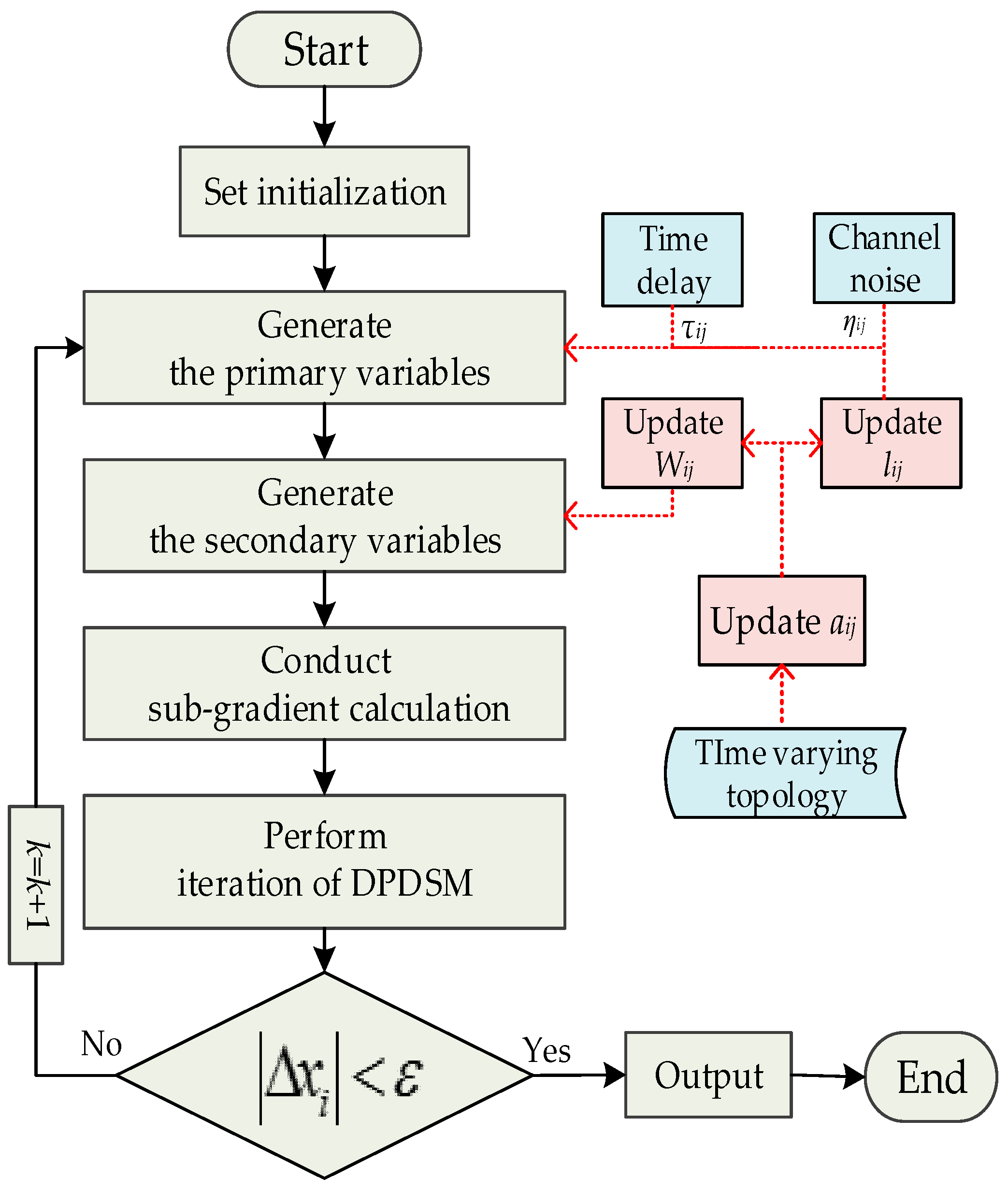
3. Distributed Primal-Dual Sub-Gradient Method (DPDSM)

According to the principle of Lagrange multiplier method [16], the optimal solution L(x*, λ*) in Equation (12) is also the optimal solution x* in the original optimization problem (Equation (2)). In order to obtain the optimal solution quickly, the method of DPDSM is adopted in this paper.

3.1. Under Ideal Communication Network Conditions

During the DPDSM iteration, the primary variables (with the symbol “^”) and secondary (with the symbol “-”) variables are derived from the original variables xi, λi:
x i ^ [ k ] = j = 1 n [ W Δ ] i j x j [ k ] λ i ^ [ k ] = j = 1 n [ W Δ ] i j λ j [ k ]
x i ^ [ 0 ] = x i [ 0 ] ,   x i ^ [ Δ + N ] = x i ^ [ Δ ] λ i ^ [ 0 ] = λ i [ 0 ] ,   λ i ^ [ Δ + N ] = λ i ^ [ Δ ]
x i ¯ [ k + 1 ] = j = 1 n [ W Δ ] i j x j ^ [ k ] λ i ¯ [ k + 1 ] = j = 1 n [ W Δ ] i j λ j ^ [ k ]
where k ≥ 0 is the iteration number; Δ is the derivation times and N is the number of iteration conducted by the original variables. That is, setting the value of Δ can adjust the engagement of consensus algorithm in the distributed optimization. Wn×n is the n order communication matrix and its element Wij is calculated by the following formula:
W i j = { 1 / n , j Γ ( i ) 1 j Γ ( i ) W i j , i = j 0 , j Γ ( i ) , j i
where n is the number of DERs which are connected with DER i by communication links. Γ (i) is the set of DERs which are connected with DER i by communication links.
L x i ( x i ¯ [ k + 1 ] , λ i [ k ] ) = S f i ( x i ¯ [ k + 1 ] ) + s = 1 q S h s ( x i ¯ [ k + 1 ] ) λ i [ k ] L λ i ( x i [ k ] , λ i ¯ [ k ] ) = h ( x i [ k ] )
where Lxi(xi[k], λi[k]) is the partial derivatives of xi[k] at (xi[k], λi[k]) and Lλi(xi[k], λi[k]) is the partial derivatives of λi[k] at the same point. The sub-gradient value of fi and hs at xi[k] are Sfi (xi[k]) and Shs (xi[k]), respectively:
x i [ k + 1 ] = P X [ x i ¯ [ k + 1 ] α L x i ( x i ¯ [ k + 1 ] , λ i [ k ] ) ] λ i [ k + 1 ] = P ˄ [ λ i ¯ [ k + 1 ] + α L λ i ( x i [ k ] , λ i ¯ [ k + 1 ] ) ]
where ˄ is the set of λi; the iteration step is α. PX and P˄ are symbols of the projection operator whose definition and principle has been given in [17].

3.2. Under Non-Ideal Communication Network Conditions

As mentioned in the introduction, the non-ideal communication network conditions consist of communication time delays, channel noises, DERs’ power output over-limit, DERs’ plug-and-play, and channel faults. The primary and secondary variables introduced in the proposed method are all auxiliary variables. All of the non-ideal communication network conditions will exist and be addressed in the primary variables, and the time varying topology events are mainly addressed in the secondary variables:
x i ^ [ k ] = x i [ k ] c [ k ] j = 1 n l i j [ k ] ( x j [ k τ i j ( k ) ] + η i j [ k ] ) λ i ^ [ k ] = λ i [ k ] c [ k ] j = 1 n l i j [ k ] ( λ j [ k τ i j ( k ) ] + η i j [ k ] )
x i ¯ [ k + 1 ] = j = 1 n [ W Δ ] i j x j ^ [ k ] λ i ¯ [ k + 1 ] = j = 1 n [ W Δ ] i j λ j ^ [ k ]
where k ≥ 0 is the iteration number; τij(k) and ƞij[k] are the time delays and channel noises from agent j to i at iteration k, respectively. c[k] is the gain function [3] and its details are described in the Appendix A.
a i j [ k ] = { 1 ,   i   is   connected   to   j 0 ,   otherwise
The adjacency matrix based on the communication topology has the element of aij. If there exists a communication link between i and j, the value of aij will be 1; otherwise, the value of aij will be 0. lij represents the Laplacian matrix element in the network topology and it is relevant to the adjacency matrix element aij.
{ l i j = a i j [ k ] l i i = j Γ ( i ) a i j [ k ]
Wn×n can be designed as a dynamic matrix under the non-ideal network conditions and the Wij is calculated by a new formula:
W i j = { 1 / j Γ ( i ) a i j , j Γ ( i ) 1 j Γ ( i ) W i j , i = j 0 , j Γ ( i ) , j i
where n is the number of DERs which are connected with DER i by communication links. Γ(i) is the set of DERs which are connected with DER i by communication links.
According to [3,9], the changes of Laplacian matrix and communication matrix can reflect the situation of the time varying topology. The flowchart of DPDSM, considering the non-ideal network conditions, is shown in Figure 1. The left part of Figure 1 displays the basic progress of the proposed algorithm; the right part provides details about how non-ideal network conditions influence the distributed dispatch. When time varying topology occurs, the value of aij will be updated according to the actual communication topology. Then, the Laplacian matrix and communication matrix will be updated along with aij. If there are time delays and channel noises in the communication lines, the dispatch will also be affected.

4. Numerical Examples

In this paper, to verify the validity of the proposed VPED strategy, two VPP systems are built by modifying the IEEE-34 bus test system and the IEEE-123 bus test system, respectively. In this work, the power error tolerance ε in Figure 1 is 0.05 kW and the iteration step α is set to 0.002 s. For the convenience of simulation, the gain function c[k] is 0.5[1 + ln(k + 1)]/(k + 1) which can meet the conditions in the Appendix A. The algebraic sum of power flowing through PCC is Ps and the total loads are recorded as PD. The purchase price θ is 0.076$/kWh and the sale price β is 0.072$/kWh. The parameters and the capacity limits of DERs are listed in Table 1 and Table 2, respectively.
The simulation implemented on the modified IEEE-34 bus test system is mainly designed to study the impact of communication time delays and channel noises on the distributed dispatch and the influence of changing Δ over the distributed dispatch algorithm. The modified IEEE-123 bus test system is aimed to investigate the adaptability of the distributed VPED algorithm under a large scale non-ideal communication network. It primarily discusses the time varying communication topology conditions arising from channel faults of communication links, DERs’ over-limit, and DERs’ plug-and-play.

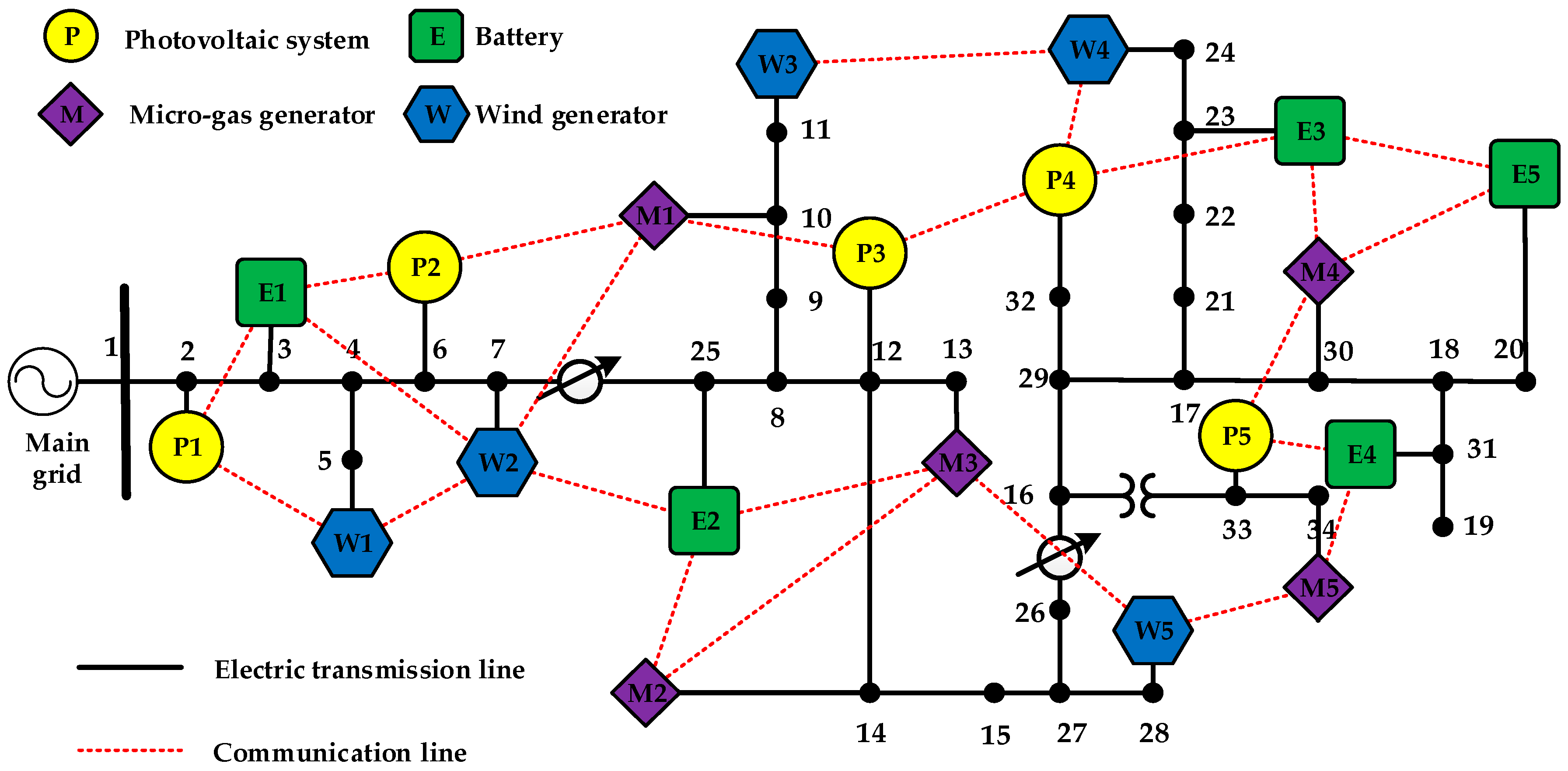
4.1. The Modified IEEE-34 Bus Test System

As shown in Figure 2, there are twenty schedulable DERs in the modified IEEE-34 bus test system. For the sake of making better use of renewable energies, PVs, and WGs will operate at their maximum power output. BEs can work in both charging and discharging modes and the MGGs may reduce their outputs to cut the fuel expenditure. BEs and MGGs are also able to adjust their outputs to deal with some unexpected events, which is aimed to maintain the system power balance. In comparison, Table 3 offers the results optimized by using the centralized dispatch under the same operation condition and Table 4 shows VPP’s average profits made by the two dispatch strategies. Three scheduling scenarios are provided as follows: (A) a distributed dispatch under the ideal communication network; (B) a distributed dispatch considering time delays and channel noises in communication network; and (C) a distributed dispatch with a different Δ.

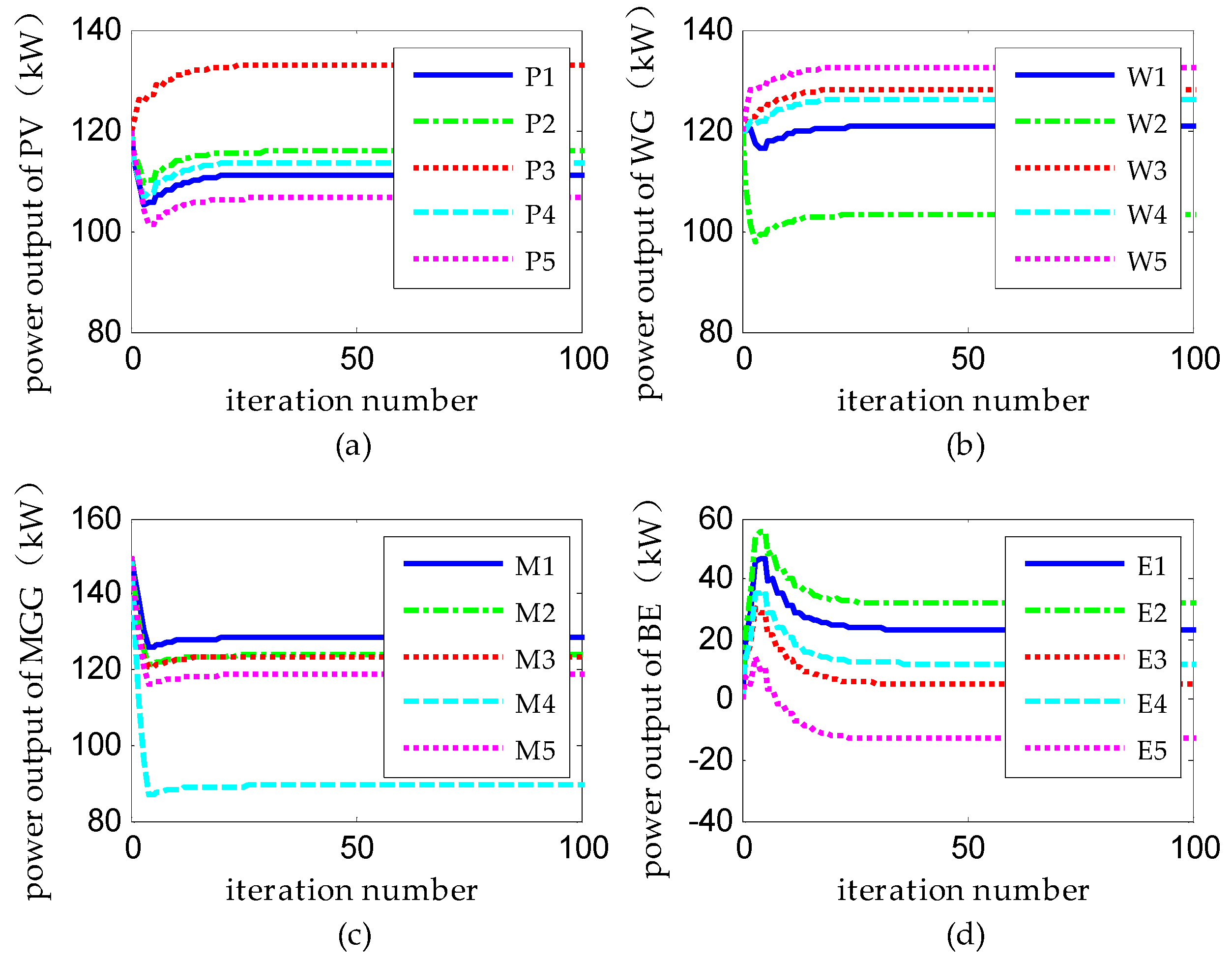
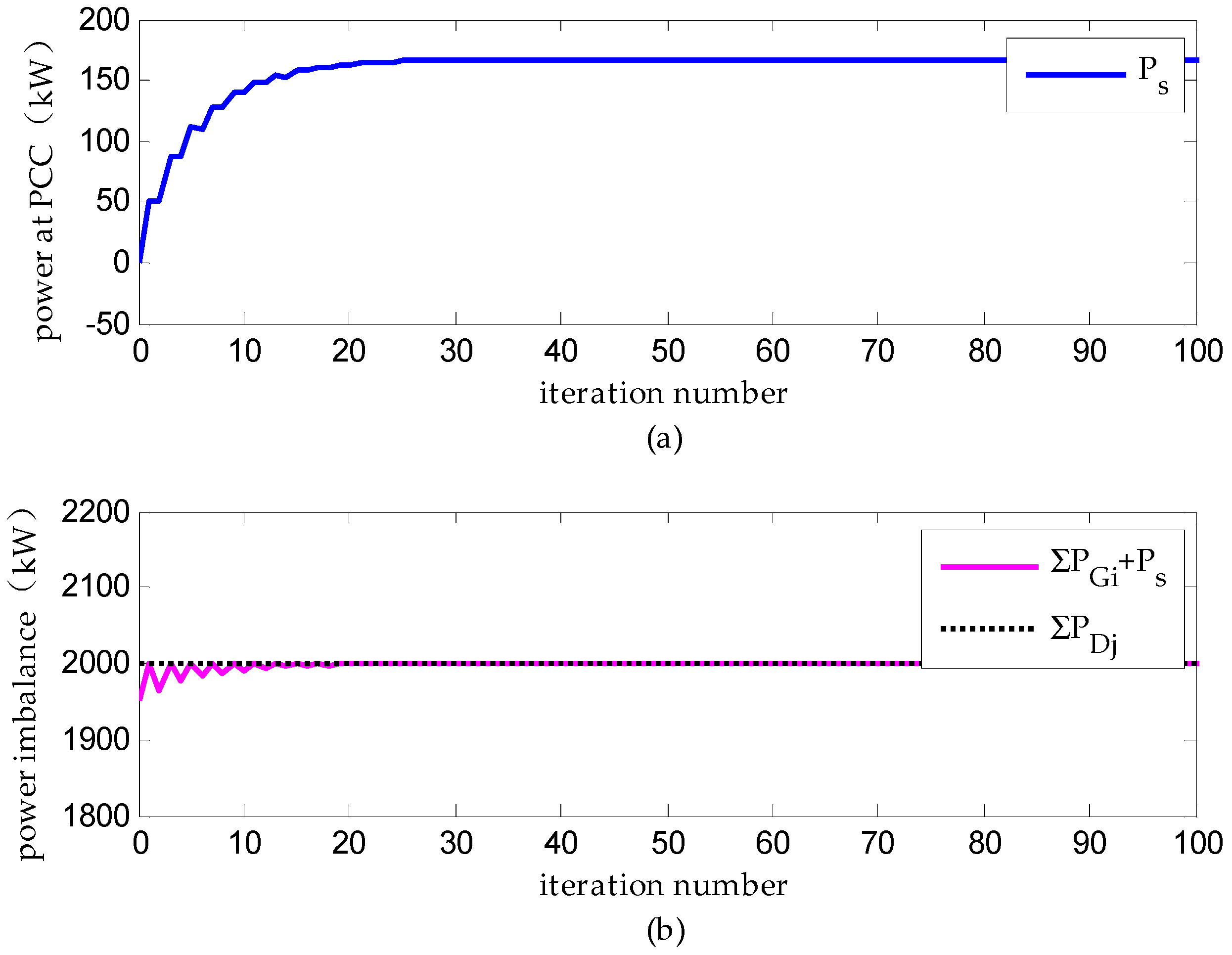
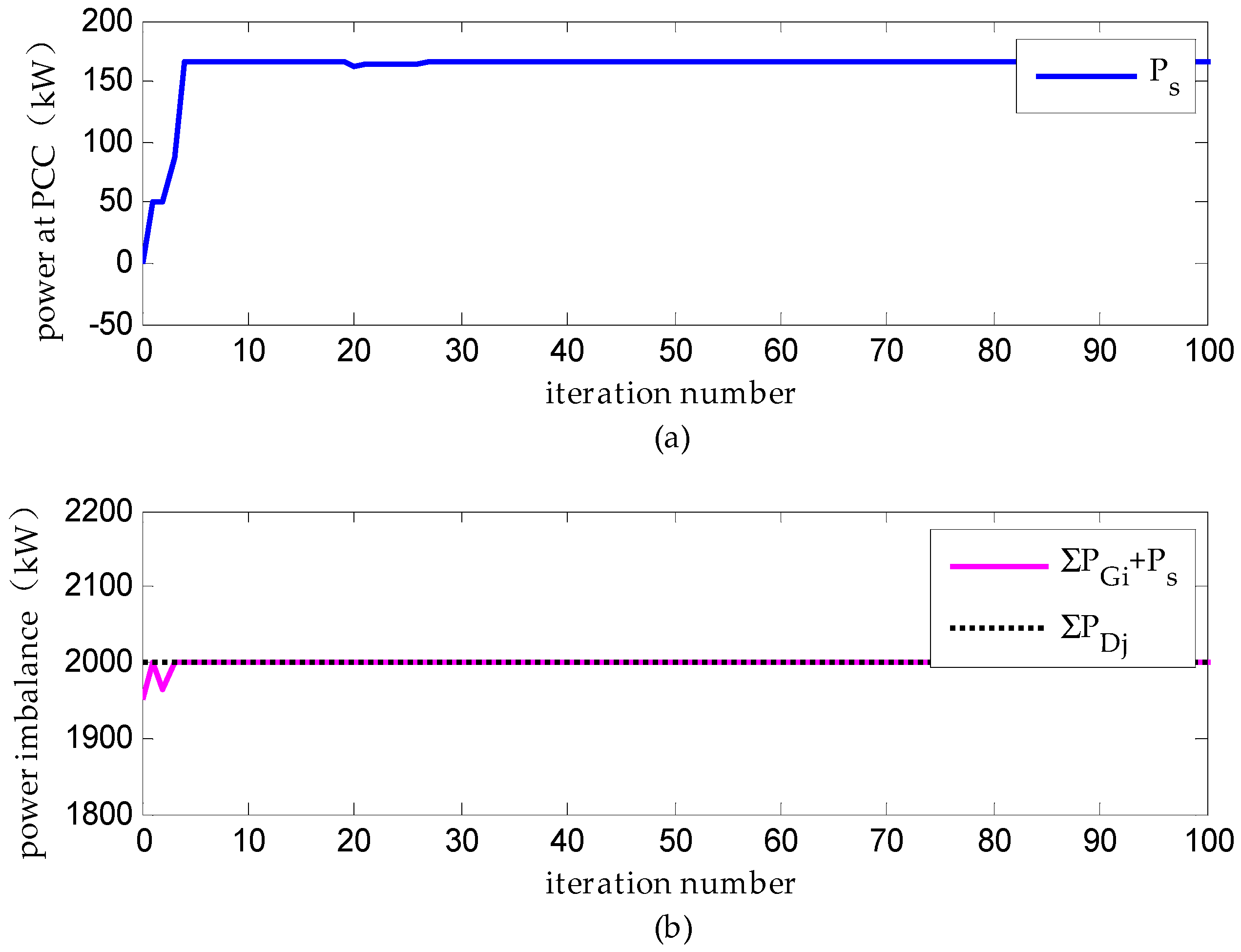
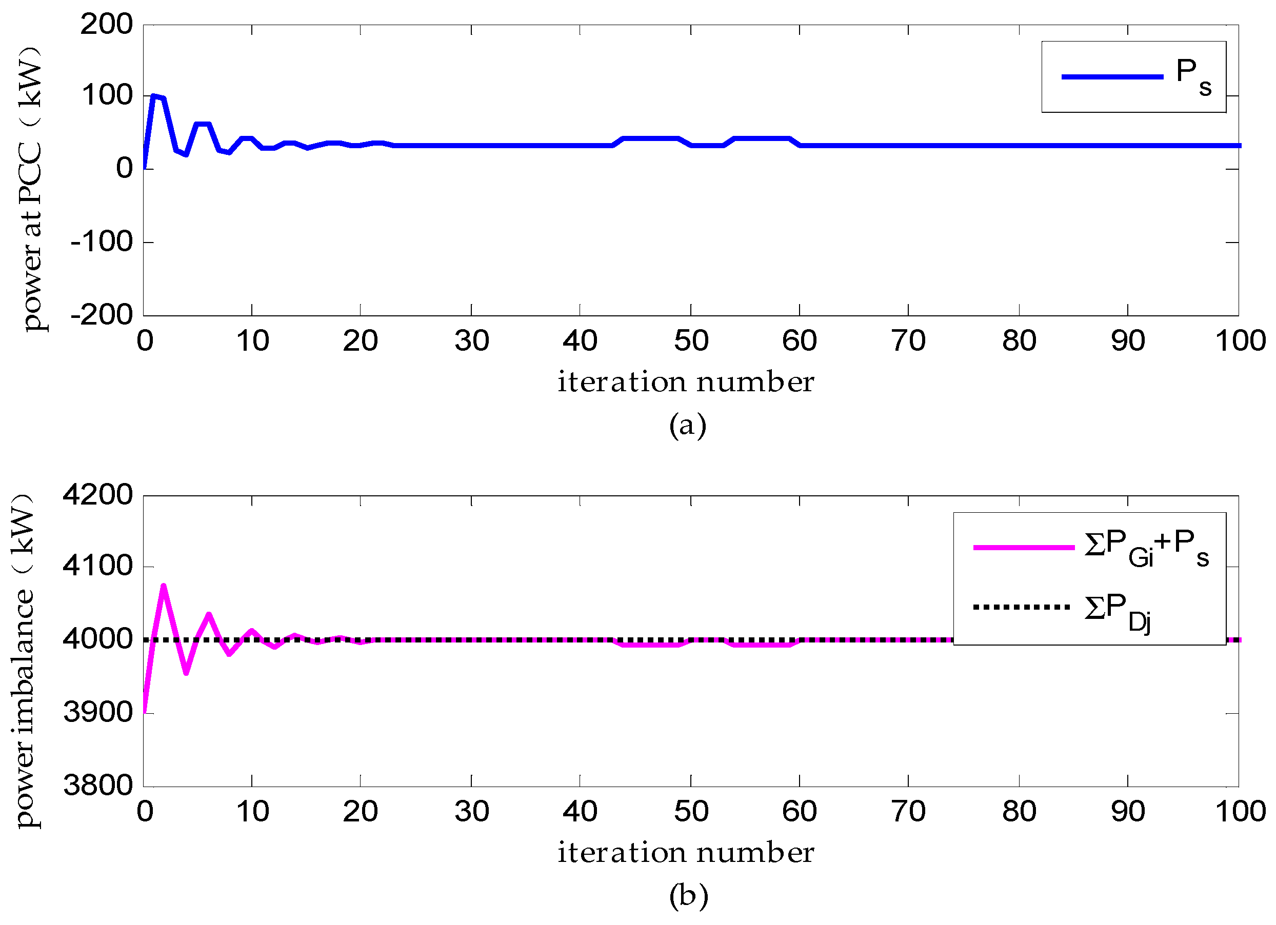
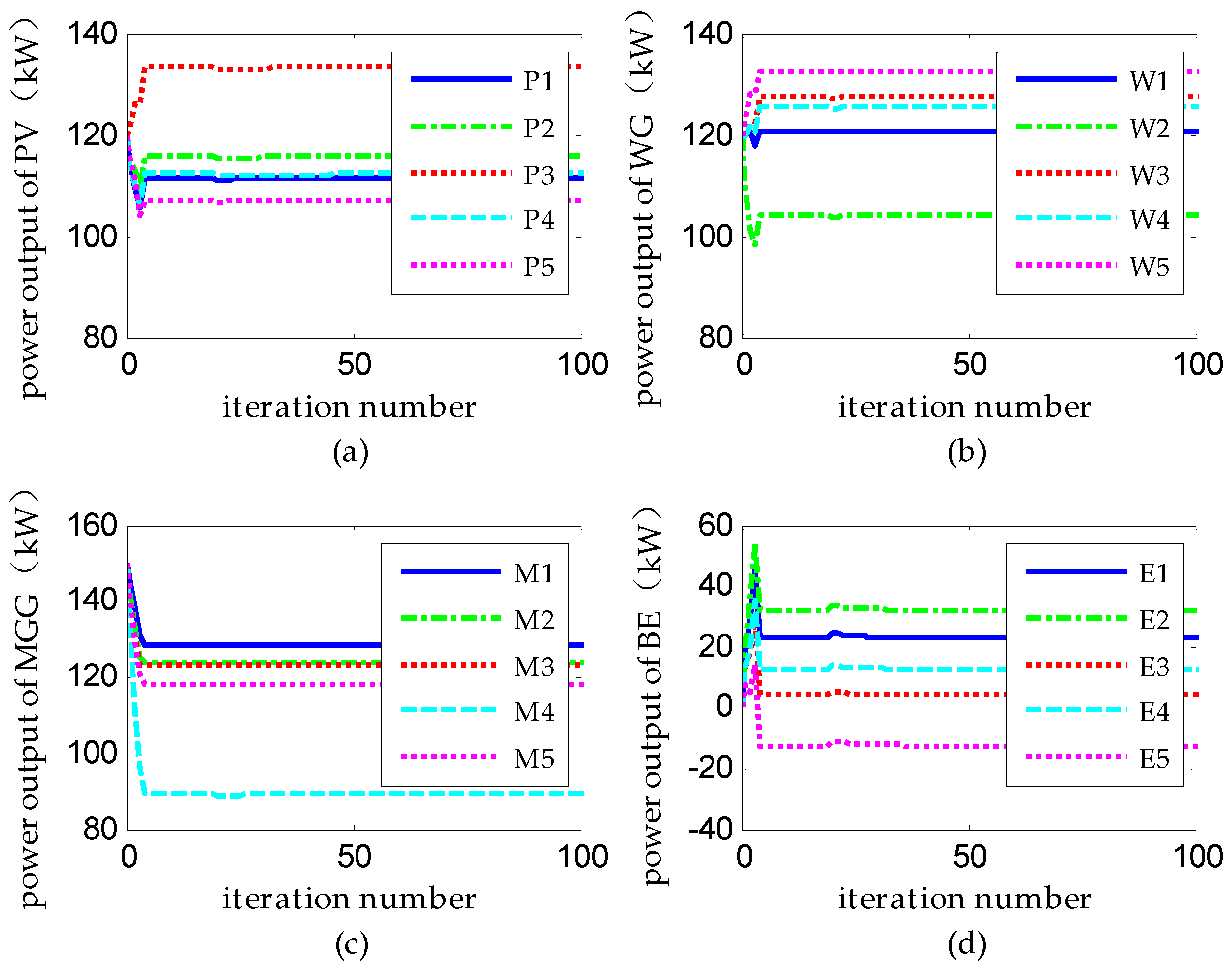
(1) Scenario A: Distributed Dispatch under Ideal Communication

Figure 3 indicates the optimal scheduling results of each DER and Figure 4 provides the variation of Ps during the distributed optimization process. From Figure 3 and Table 3, we can find that the distributed dispatch proposed in this paper achieves the same scheduling scheme as the centralized dispatch does, which shows the effectiveness of the distributed dispatch strategy. From the viewpoint of profits, it is not difficult to find in Table 4 that the distributed dispatch is the same with the centralized one. Figure 4 illustrates that the VPP can sell electric energy to the main grid when its overall power is higher than load demands, but if the overall power is lower than the total loads, VPP will absorb power from the main grid to maintain the supply-demand balance.

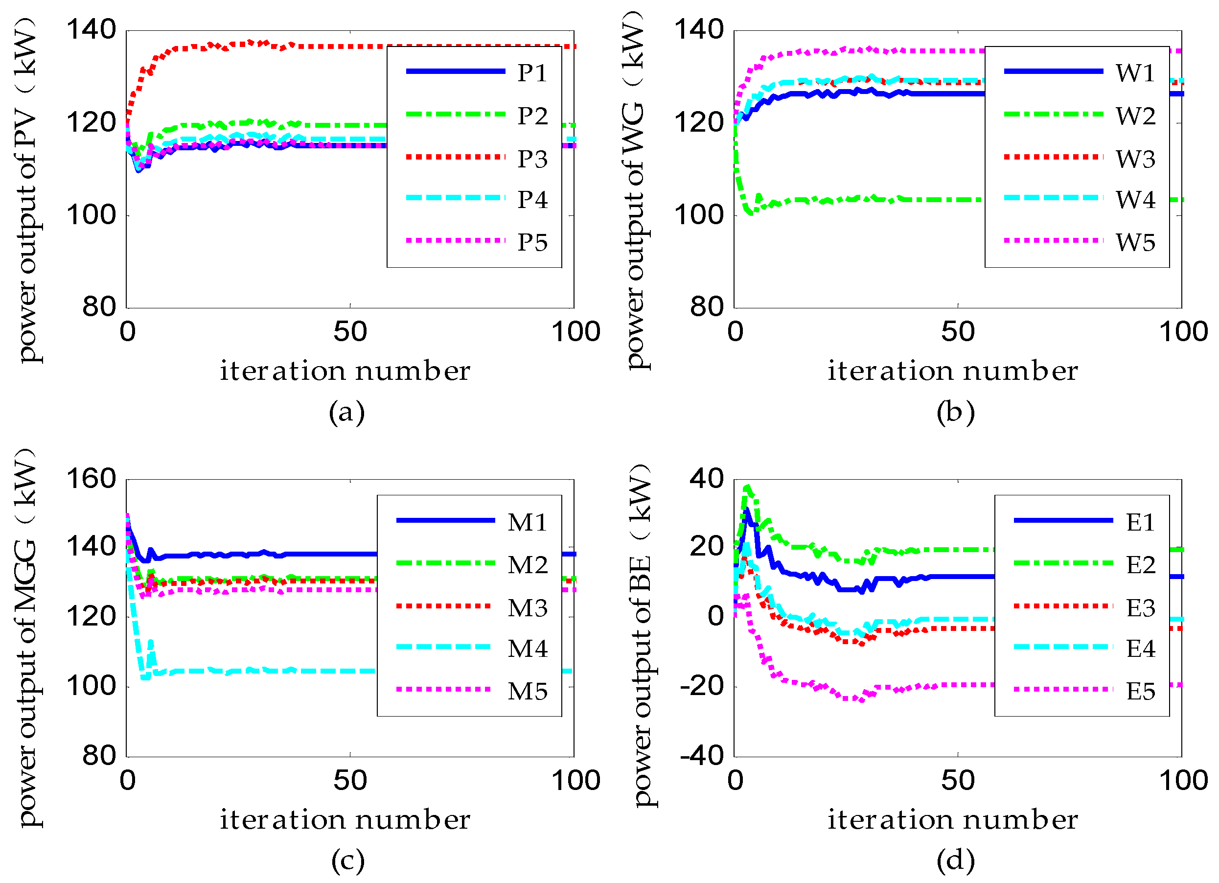
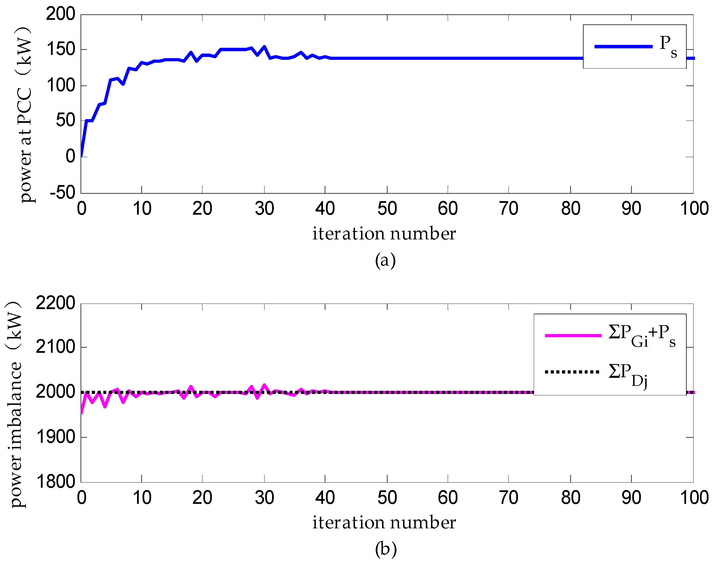
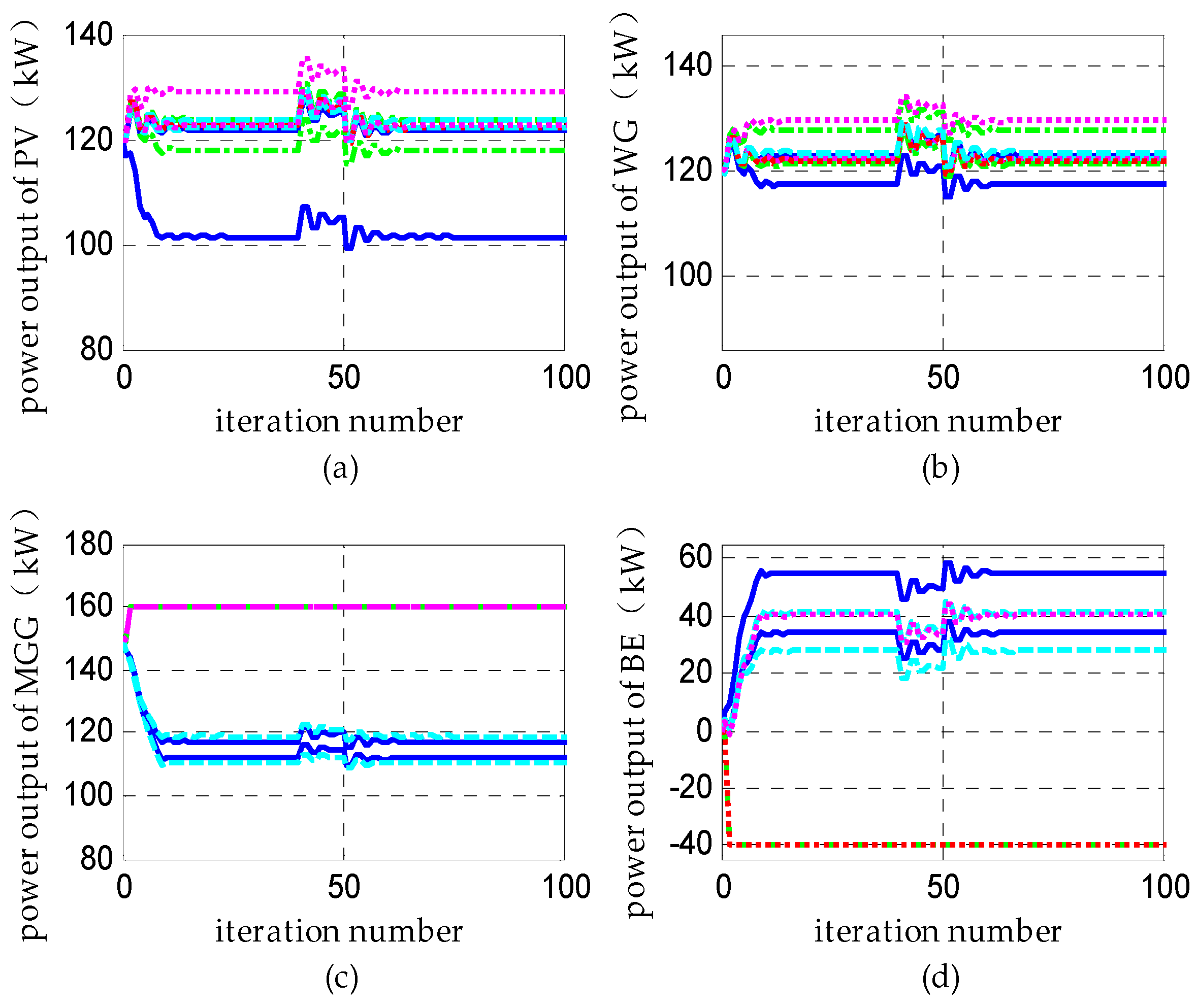
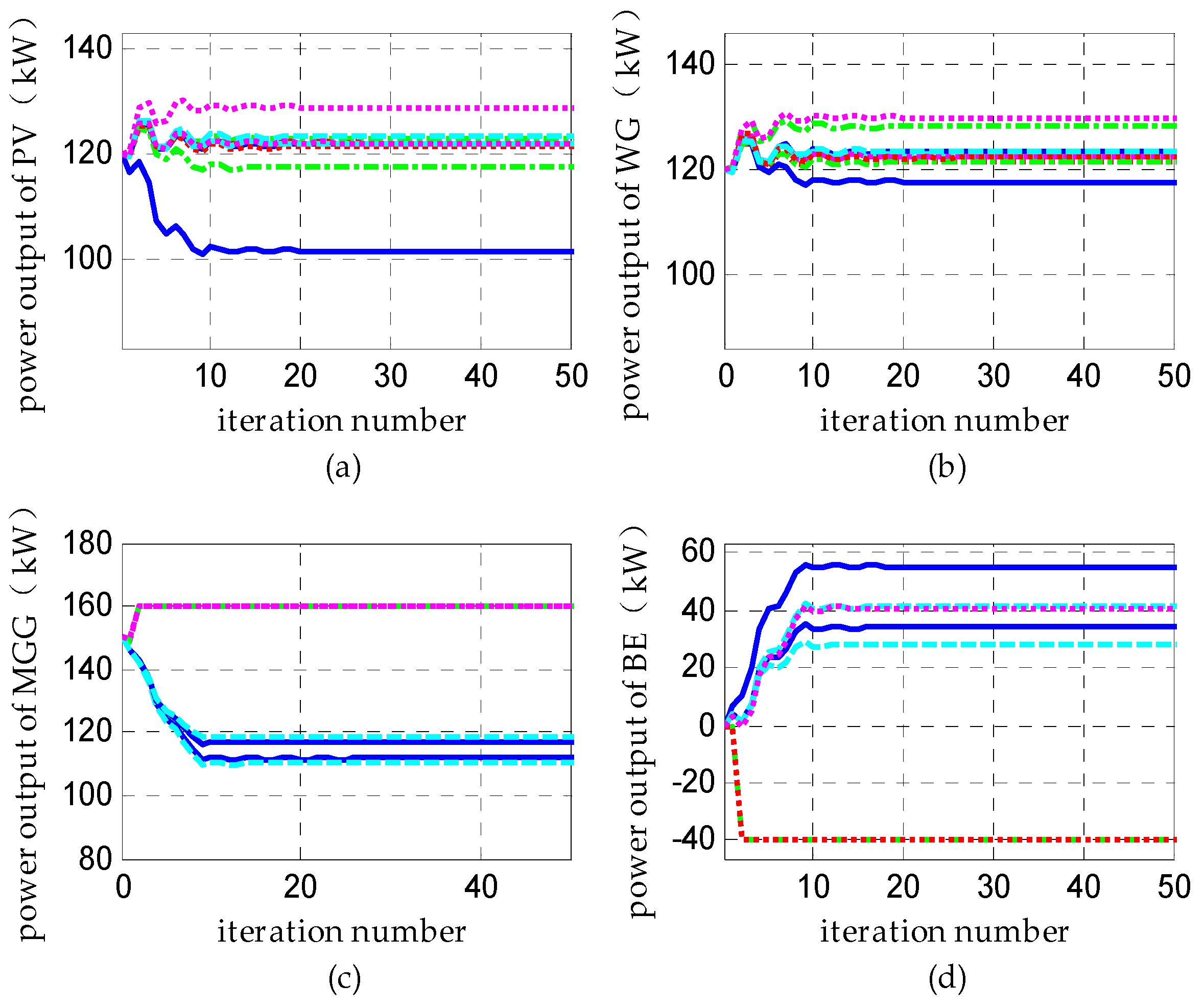
(2) Scenario B: Distributed Dispatch Considering Communication Time Delays and Channel Noises

In practice, it is necessary to consider communication time delays and channel noises. When implementing the optimization, the delays are randomly distributed between 0 and 3; meanwhile, the noises are randomly distributed between 0 and 5 kW. Figure 5 shows the optimization curves of this scenario. Figure 6 provides the variation of Ps and the power imbalance during the optimization. Since the transmission of the iteration information is postponed by time delays, curves for showing the variation of Ps and the power imbalance will appear in cross-sections, such as M1 in Figure 5c. Channel noises will cause the oscillation of power outputs; for example, M4 from the 16th to the 25th iterations. The more serious the delays and noises are, the rougher the curves will be. By the aid of the main grid, VPP can shrink the whole fluctuation and keep the system power balance (see Figure 6). In the centralized scheduling, prediction of communication time delays and channel noises is needed and it will increase the scheduling burden. Based on the local communication mechanism, the proposed method can still reach the same result, but in a way of real-time scheduling, meaning that the proposed method is useful to improve the system noise immunity. The simulation shows the effectiveness of the distributed scheduling strategy in handling time delays and channel noises.

(3) Scenario C: Distributed Dispatch with a Different Δ

Changing the value of Δ means adjusting the consensus parameters in the distributed dispatch. Δ is set at 3 in scenario a while Δ is set at 10 in this scenario. Contrasting Figure 7 and Figure 8 with Figure 3 and Figure 4, it is clear that the larger the value is, the faster the convergence speed, but the larger the oscillation that will be occurred in the optimization.

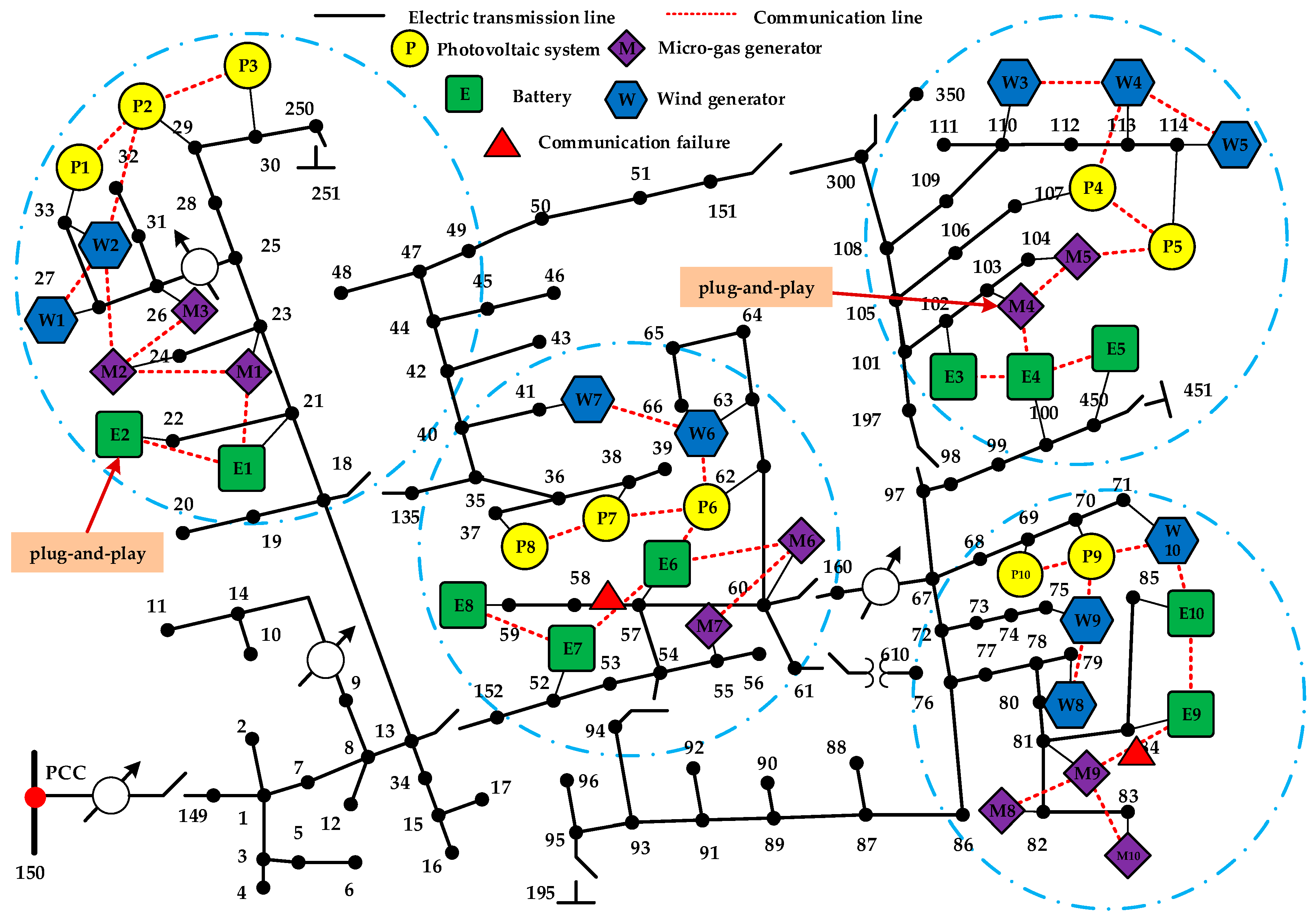
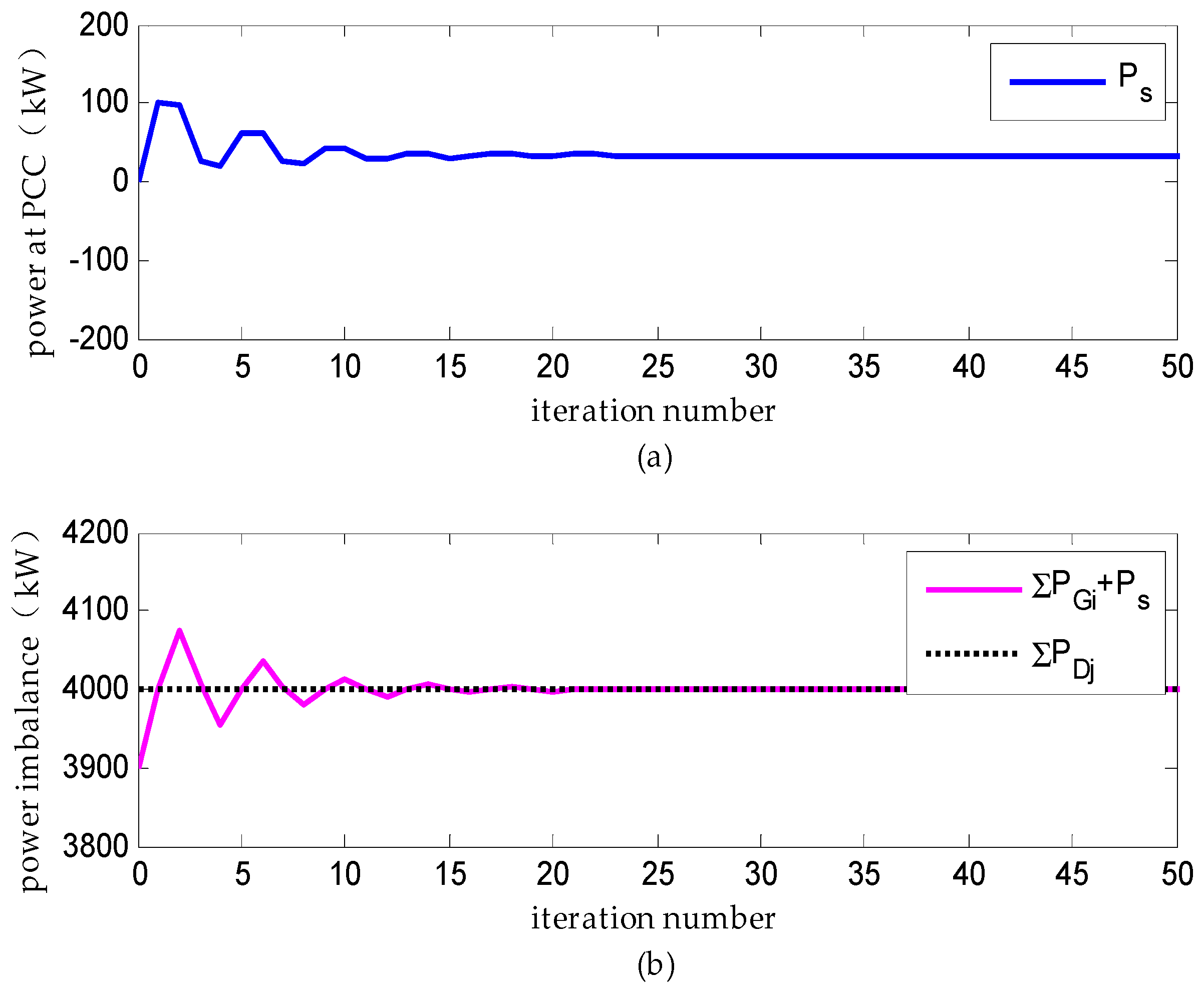
4.2. The Modified IEEE-123 Bus Test System

The modified IEEE-123 bus test system is shown in Figure 9. In this example, forty DERs are dispersed in four areas in this test system. The operation parameters are the same with the previous test system. Three simulation scenarios are implemented as follows: (D) a distributed dispatch under the condition of the DERs’ over-limit; (E) a distributed dispatch under the condition of channel faults; and (F) a distributed dispatch under the condition of DERs’ play-and-plug.

(1) Scenario D: Distributed Dispatch under the Condition of DERs’ Over-Limit

In order to ensure the safe operation of the VPP, it is essential to consider the capacity limits of DERs. Suppose a few MGGs’ and BEs’ power outputs have reached the limits during the optimization. Figure 10 shows that the over-limit DERs will run at the power limit and no longer iterate in the optimization, but continue to deliver data to their neighbors. Based on this local communication mechanism, the over-limit DERs may only affect the adjacent DERs rather than the whole. Figure 11 indicates that, with regard to DERs’ over-limit events, the distributed method can still maintain the system power balance constraint.

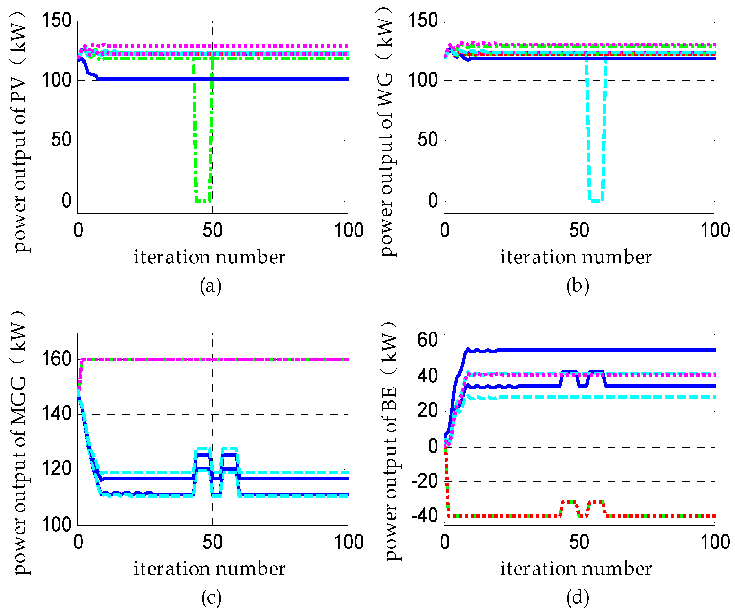
(2) Scenario E: Distributed Dispatch under the Condition of Channel Faults

Channel faults will lead to the change of the communication topology. After the wrong channels are removed, the system recovers its power balance by reconstructing a new communication topology. The damaged channels are shown in Figure 9 and the dispatch progress is displayed in Figure 12 and Figure 13. The channel faults can disturb DERs’ normal operation. Then, the system will build a new stable state by distributed VPED optimization.

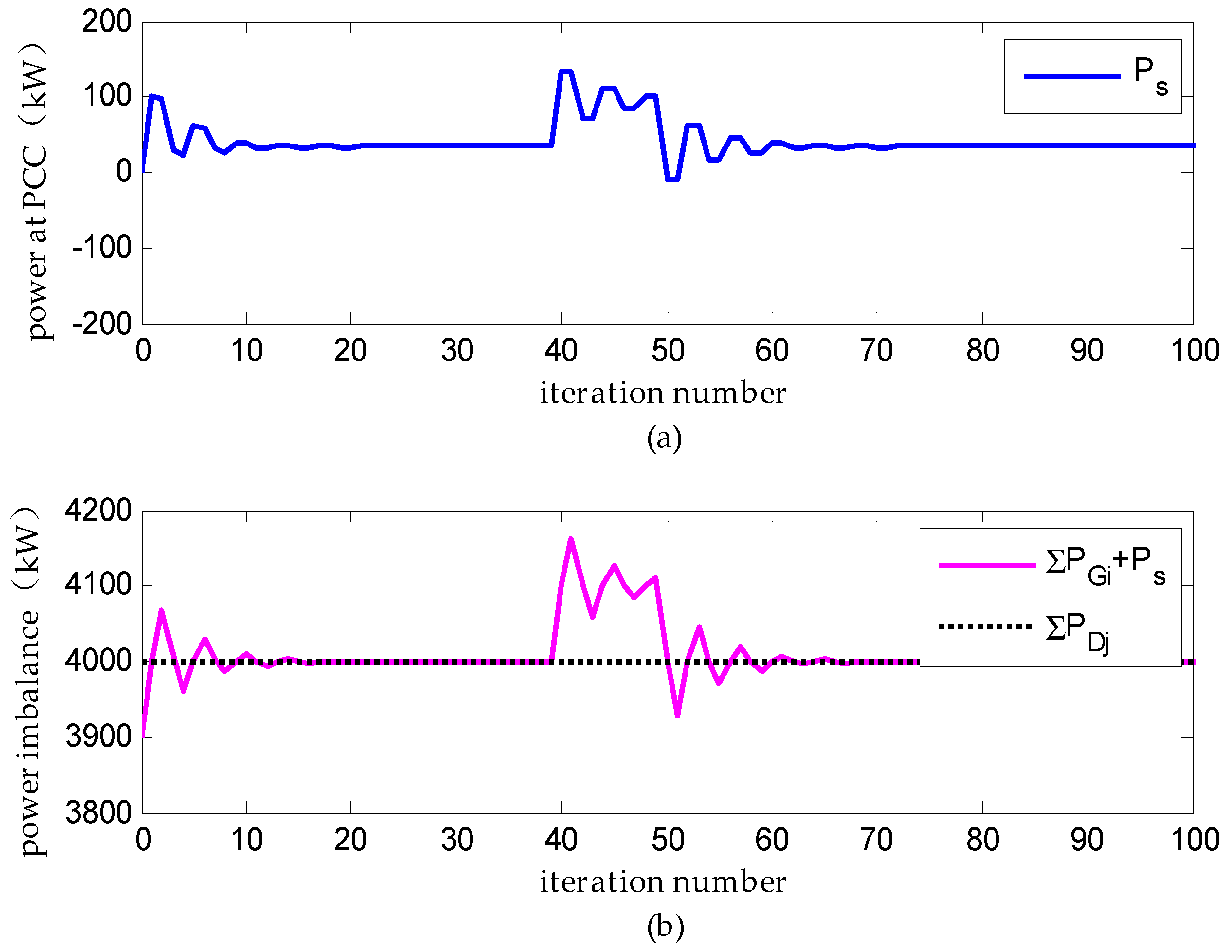
(3) Scenario F: Distributed Dispatch with DERs’ Plug and Play

Compared with non-ideal communication conditions, DERs’ plug-and-play is most likely to occur under an actual large-scale VPP system. There are two DERs that temporarily plug-and-play during the distributed scheduling in this scenario. From Figure 14, we can see that a PV plug off at about the 45th iteration for some reasons, but plug on at about the 50th iteration. However, by adjusting the power of MGGs, Bes, and Ps, the VPP system immediately realizes a new supply-demand power balance (see Figure 15). When this event happens again on a WG, the VPP system still restores its stability within a short time. Faced with the DER plug-and-play conditions, the system employing the proposed method in this paper shows a strong robustness.

5. Summary

The VPP is often adopted to manage large-scale DERs but there are non-ideal conditions of the communication network during its economy dispatch. With the consideration of various constraints, communication time delays, channel noises, and time varying topology, this paper establishes a VPP dispatch model and proposes a DPDSM to solve it. Compared with the centralized method under the same simulation scenarios, it can be found that the VPP can integrate DERs effectively and economically. Simulation results show that the larger communication time delays and channel noises are, the more unstable the system is. The frequent-and-diverse time varying topology events can also disturb its steady operation. The DPDSM can converge fast in the scheduling process and respond quickly to these non-ideal communication conditions. Simulations analysis illustrates the validity and superiority of the proposed method. Some issues, such as the sensitivity of the results to parameters, VPP’s multi-period dispatch, etc., still need further exploration.

Acknowledgments

This study is supported by the National Science Foundation of China (Grant No. 51577051) and the Major State Basic Research Development Program of China (Grant No. 2016YFB0901101), and the Innovation Research Foundation of Graduate Students of Jiangsu Province (Grant No. SJLX15_0385, SJLX16_0330, SJLX16_0332).

Author Contributions

All of the authors contributed to this work. Chi Cao designed the study, developed the mathematical model, and performed the analysis and simulations. Jun Xie provided critical guidance to this research and checked the overall logic of this work. Dong Yue contributed to the conceptual approach on the modeling and analysis. Chongxin Huang contributed towards the non-ideal communication conditions. Jixiang Wang contributed towards the modeling framework. Shuyang Xu contributed towards the DPDSM. Xingying Chen provided important comments on the modeling and analysis.

Conflicts of Interest

The authors declare no conflict of interest.

Appendix A

The output models of WGs, PVs, and BEs can be formulated as follows:
(a)
Wind generators [23]. The power outputs of WGs are mainly affected by the wind speed and they can be described by the linear model:
P w = { 0 v < v c i , v v c o v v c i v r v c i P r v c i < v < v r P r v r v v c o
where Pw is the maximum available power output and Pr is the rated power output of WGs. v, vci, vco, and vr are wind speeds, cut-in wind speeds, cut-out wind speeds, and the rated wind speeds, respectively.
(b)
Photovoltaic systems [24]. The PVs’ power outputs are mainly affected by the light intensity and temperature, and the model can be expressed as:
P PV = P PV max G C G C max [ 1 + K ( T c T r ) ]
where PPV is the maximum available power output of PVs, and P PV max represents the maximum output under standard test conditions. GC means the actual light intensity; GCmax is the reference one under standard test conditions. The conversion coefficient of temperature to power is depicted by K. Tc, Tr is the environment temperature and the reference temperature under standard test conditions, respectively.
(c)
Storage batteries [10]. In this model, the constraints are mainly considered:
{ P BE P BE d c h max , P BE 0 P BE P BE c h max , P BE 0
where PBE ≥ 0 states the actual power output in the discharging and P BE d c h max represents the maximum power output. Consequently, PBE ≤ 0 and P BE c h max can be the same one with the charging state. The state-of-charge (SOC) is also an important constraint. The charging efficiency of BE will be very low if the SOC come to a critical value. To solve the problem, the following formulas are given as:
P BE = { P BE d c h , S O C S O C u p P BE d c h   o r   P BE c h , S O C u p S O C S O C d o w n P BE c h , S O C d o w n S O C
where SOCup and SOCdown are the lower bound and upper bound of BE. This study investigates the transient process of the distributed scheduling, so BEs can work at the two states during this period.
We mainly study DERs’ economy scheduling and some parameters of DERs’ outputs models will be listed in Table A1.
In order to ensure the convergence of the algorithm, the c[k] needs to meet the following necessary conditions [25]:
{ k = 0 c [ k ] = + k = 0 c 2 [ k ] < +
According to reference [3], the c[k] is designed as:
c [ k ] = 0.5 [ 1 + ln ( k + 1 ) ] / ( k + 1 )
where 0 is the delay coefficient. Xu et al. [3] concluded that the optimization will become faster as the coefficient value gets smaller.
Table A1. Parameters of DERs’ outputs models.
ParametersValues
Cut-in wind speeds vci3.0 m/s
Cut-out wind speeds vco25 m/s
The rated wind speeds vr15 m/s
The rated power output Pr200 kW
The capacity of BE100 kWh
SOCup80%
SOCdown20%
PPVmax200 kW
GCmax1 kW/m2
The coefficient Kin (25)−0.45%
Tr25 °C

References

  1. Malahat, P.H.; Seifi, H.; Eslami, S.E. Decision making of a virtual power plant under uncertainties for bidding in a day-ahead market using point estimate method. Int. J. Electr. Power Energy Syst. 2013, 44, 88–98. [Google Scholar]
  2. Ali, Z.G.; Alireza, Z.; Shahram, J.; Kazemi, A. Stochastic operational scheduling of distributed energy resources in a large scale virtual power plant. Int. J. Electr. Power Energy Syst. 2016, 82, 608–620. [Google Scholar]
  3. Xu, H.; Zhang, X.; Yu, T. Robust consensus algorithm for economic dispatch under non-ideal communication network. Autom. Electric Power Syst. 2016, 40, 15–24. (In Chinese) [Google Scholar]
  4. Hatziargyriou, N.; Asand, H.; Iravani, R.; Marnay, C. Microgrids. IEEE Power Energy Mag. 2007, 5, 78–94. [Google Scholar] [CrossRef]
  5. Thavlov, A.; Bindner, H.W. Utilization of flexible demand in a virtual power plant set-up. IEEE Trans. Smart Grid 2015, 6, 640–647. [Google Scholar] [CrossRef]
  6. Ruiz, N.; Cobelo, I.; Oyarzabal, J. A direct load control model for virtual power plant management. IEEE Trans. Power Syst. 2009, 24, 959–966. [Google Scholar] [CrossRef]
  7. Khaled, I.H.; Saber, S.M.; Mahmoud, B.M.E. Design of multi-step LC compensator for time-varying nonlinear loads based on genetic algorithm. Int. Trans. Electr. Energy Syst. 2016, 26, 2643–2656. [Google Scholar]
  8. Amjady Ali, G.; Zakariya, H. Solution of economic load dispatch problem via hybrid particle swarm optimization with time-varying acceleration coefficients and bacteria foraging algorithm techniques. Int. Trans. Electr. Energy Syst. 2013, 23, 1504–1522. [Google Scholar]
  9. Zhang, W.; Liu, W.; Wang, X. Online optimal generation control based on constrained distributed gradient algorithm. IEEE Trans. Power Syst. 2015, 30, 35–45. [Google Scholar] [CrossRef]
  10. Yang, H.; Yi, D.; Zhao, J.; Zhao, Y.D. Distributed optimal dispatch of virtual power plant via limited communication. IEEE Trans. Power Syst. 2013, 28, 3511–3512. [Google Scholar] [CrossRef]
  11. Yang, H.; Yi, D.; Zhao, J.; Luo, F.; Zhao, Y.D. Distributed optimal dispatch of virtual power plant based on ELM transformation. Ind. Manag. Optim. 2014, 10, 1297–1318. [Google Scholar] [CrossRef]
  12. Xin, H.; Gan, D.; Li, N.; Li, H.; Dai, C. Virtual power plant-based distributed control strategy for multiple distributed generators. IET Control Theory Appl. 2013, 7, 90–98. [Google Scholar] [CrossRef]
  13. Qiu, J.; Wang, T.; Yin, S.; Gao, H. Data-based optimal control for networked double-layer industrial processes. IEEE Trans. Ind. Electron. 2016. [Google Scholar] [CrossRef]
  14. Vasirani, M.; Kota, R.; Cavalcante, R.; Ossowski, S.; Jennings, N.R. An agent-based approach to virtual power plants of wind power generators and electric vehicles. IEEE Trans. Smart Grid 2013, 4, 1314–1322. [Google Scholar] [CrossRef]
  15. Qiu, J.; Gao, H.; Steven, X. Recent advances on fuzzy-model-based nonlinear networked control systems: A survey. IEEE Trans. Ind. Electron. 2016, 63, 1207–1217. [Google Scholar] [CrossRef]
  16. Yuan, D.; Xu, S.; Zhao, H. Distributed primal–dual sub-gradient method for multi agent optimization via consensus algorithms. IEEE Trans. Syst. Man Cybern. B Cybern. 2011, 41, 1715–1723. [Google Scholar] [CrossRef] [PubMed]
  17. Angelia, N.; Asuman, O.; Pablo, A.P. Constrained consensus and optimization in multi-Agent networks. IEEE Trans. Autom. Control 2010, 55, 922–938. [Google Scholar]
  18. Zhu, M.; Martinez, S. On distributed convex optimization under inequality and equality constraints via primal–dual sub-gradient methods. IEEE Trans. Autom. Control 2011, 57, 151–164. [Google Scholar]
  19. Ali, R.M.; Mahdi, R. Optimal operating strategy of virtual power plant considering plug-in hybrid electric vehicles load. Int. Trans. Electr. Energy Syst. 2016, 26, 236–252. [Google Scholar]
  20. Rahimiyan, M.; Baringo, L. Strategic bidding for a virtual power plant in the day-ahead and real-time markets: A price-taker robust optimization approach. IEEE Trans. Power Syst. 2016, 31, 2676–2687. [Google Scholar] [CrossRef]
  21. Kardakos, E.G.; Simoglou, C.K.; Bakirtzis, A.G. Optimal offering strategy of a virtual power plant: A stochastic bi-level approach. IEEE Trans. Smart Grid 2012, 7, 794–806. [Google Scholar] [CrossRef]
  22. Liu, Y.; Xin, H.; Wang, Z.; Gan, D. Control of virtual power plant in micro grids: A coordinated approach based on photovoltaic systems and controllable loads. IET Gener. Transm. Distrib. 2015, 9, 921–928. [Google Scholar] [CrossRef]
  23. John, H.; David, C.Y.; Kalu, B. An economic dispatch model incorporating wind Power. IEEE Trans. Energy Convers. 2008, 23, 603–611. [Google Scholar]
  24. Gavanidou, E.; Bakirtzis, A. Design of a standalone system with renewable energy sources using trade off methods. IET Renew. Power Gener. 1992, 7, 42–48. [Google Scholar]
  25. Liu, S.; Xie, L.; Zhang, H. Distributed consensus for multi-agent systems with delays and noises in transmission channels. Automatica 2011, 47, 920–934. [Google Scholar] [CrossRef]
Figure 1. Flowchart of DPDSM.
Energies 10 00235 g001
Figure 2. The modified IEEE-34 bus test system in Scenario A.
Energies 10 00235 g002
Figure 3. Dispatch results in Scenario A. (a) Power output of PV; (b) Power output of WG; (c) Power output of MGG; and (d) Power output of BE.
Energies 10 00235 g003
Figure 4. The simulation of power balance in Scenario A. (a) Power at PCC; and (b) The variation of power imbalance.
Energies 10 00235 g004
Figure 5. Dispatch results in Scenario B. (a) Power output of PV; (b) Power output of WG; (c) Power output of MGG; and (d) Power output of BE.
Energies 10 00235 g005
Figure 6. The simulation of power balance in Scenario B. (a) Power at PCC; and (b) The variation of power imbalance.
Energies 10 00235 g006
Figure 7. Dispatch results in Scenario C. (a) Power output of PV; (b) Power output of WG; (c) Power output of MGG; and (d) Power output of BE.
Energies 10 00235 g007
Figure 8. The simulation of power balance in Scenario C. (a) Power at PCC; and (b) The variation of power imbalance.
Energies 10 00235 g008
Figure 9. The modified IEEE-123 bus test system in Scenario D.
Energies 10 00235 g009
Figure 10. Dispatch results in Scenario D. (a) Power output of PV; (b) Power output of WG; (c) Power output of MGG; and (d) Power output of BE.
Energies 10 00235 g010
Figure 11. The simulation of power balance in Scenario D. (a) Power at PCC; and (b) The variation of power imbalance.
Energies 10 00235 g011
Figure 12. Dispatch results in Scenario E. (a) Power output of PV; (b) Power output of WG; (c) Power output of MGG; and (d) Power output of BE.
Energies 10 00235 g012
Figure 13. The simulation of power balance in Scenario E. (a) Power at PCC; and (b) The variation of power imbalance.
Energies 10 00235 g013
Figure 14. Dispatch results in Scenario F. (a) Power output of PV; (b) Power output of WG; (c) Power output of MGG; and (d) Power output of BE.
Energies 10 00235 g014
Figure 15. The simulation of power balance in Scenario F. (a) Power at PCC; and (b) The variation of power imbalance.
Energies 10 00235 g015
Table 1. Parameters of DERs.
DERs Types C i ( P G i ) = a i P G i 2 + b i P G i + c i ($/kWh)PGi[0] (kW)
ai (10−6)bi (10−3)ci
P11.1821.4980.0914120
P21.7931.3420.0945120
P31.8841.2620.0968120
P41.9161.3280.0953120
P51.9221.3470.0938120
W11.3531.4330.0840120
W21.1711.5170.0803120
W31.0731.4840.0865120
W41.6121.3560.0889120
W51.4051.3880.0840120
M16.1450.1870.1011150
M26.9320.0450.1003150
M36.6420.1280.1063150
M46.5030.5820.1006150
M56.6050.1990.1023150
E12.5031.6450.07030
E22.5491.5980.07470
E32.6071.7310.07200
E42.7201.6940.07860
E52.2401.8120.07650
Table 2. Capacity limits of DERs.
DERs TypesPGi (kW)DERs TypesPGi (kW)Capacity (kWh)
MinMaxMinMax
P1–P580140(charging)040100 kWh
W1–W580140E1–E5----------------
M1–M580160(discharging)060100 kWh
Table 3. Optimal dispatch results under the centralized dispatch.
DERs TypesScenarios
abc
P1111.103114.669111.103
P2115.680119.308115.680
P3132.903136.246132.903
P4113.546116.424113.546
P5106.496115.105106.496
W1120.632126.149120.632
W2103.116103.114103.116
W3128.165128.749128.165
W4126.303128.884126.303
W5132.594135.245132.594
M1128.314137.949128.314
M2123.691131.12123.691
M3123.509130.143123.509
M489.1574104.54889.1574
M5118.528127.819118.528
E123.230611.496723.2306
E231.717519.598731.7175
E35.24299−3.42075.24299
E411.9249−0.729611.9249
E5−13.1192−19.7492−13.1192
Ps167.259137.325167.259
Table 4. VPP’s average profits made by the two dispatch strategies.
ScenariosThe Centralized DispatchThe Distributed Dispatch
a0.0649 ($/kWh)0.0649 ($/kWh)
b0.0645 ($/kWh)0.0645 ($/kWh)
c0.0649 ($/kWh)0.0649 ($/kWh)

