Investigation of a Diesel-Engined Vehicle’s Performance and Emissions during the WLTC Driving Cycle—Comparison with the NEDC

Abstract

The present work presents results from an experimentally validated simulation code, regarding a turbocharged diesel-powered vehicle running on the recently developed worldwide light-duty vehicles WLTC driving cycle. The simulation is based on an engine mapping approach, with correction coefficients applied vis-à-vis the transient discrepancies encountered. Both performance and engine-out emission results are presented and discussed. As regards the latter, the concerned pollutants are soot and nitrogen monoxide. Since the WLTC driving cycle is scheduled to replace the NEDC in Europe from September 2017 with regard to the certification of passenger cars and light-duty trucks, a comparative analysis between the two test schedules is also performed for the engine/vehicle under study.

1. Introduction

For many decades now, the certification procedure for new vehicles (or engines) around the world is accomplished by applying a driving (or engine) cycle. By doing so, a broad range of the engine’s speed and torque is under test, as well as its transient behavior. A certification test cycle is characterized by relatively long duration (of the order of 20–30 min) consisting of both speed and load changes under varying operating conditions, cold or hot starting, including (for highway engines/vehicles) urban as well as motorway driving. Applying a driving cycle for the certification of new vehicles/engines means that simulation of the most frequent daily driving (transient) conditions is encompassed in the certification procedure [1].

When developing new engines/vehicles, internal combustion engine manufacturers are facing a two-fold challenge. Firstly, they must meet the stringent emission limits imposed by the regulations with respect to the legislated cycle; at the same time, they strive to address customer needs for vehicles with increased power and torque (good drivability) and low fuel consumption. In order to fulfill these often-conflicting tasks, the diesel engine has gradually surfaced as a rather promising alternative to the spark ignition (SI) engine. Contributing factors are its superior fuel efficiency and torque, its inherent capability to operate turbocharged as well as its reliability [2]. However, there are certain aspects of a turbocharged diesel engine’s operation that might prove particularly demanding or even problematic. The most notable one is its transient behavior, being linked with off-design operation, owing to the turbocharger lag, and therefore non-optimum performance in terms of both drivability and engine-out emissions [3,4].

Since the early 1970s, the modeling and the experimental investigation of the thermodynamic and gas dynamic processes of diesel engines has furthered the study of their transient operation. Unfortunately, the vital issue of exhaust emissions, as well as the overall engine and vehicle performance during driving cycles, has not been investigated in a thorough and comprehensive manner, owing mainly to two reasons. Firstly, it is the inherent difficulties involved in developing and validating multi-zone simulation models that require huge computational time for the reproduction of a driving cycle. Secondly, costly and sophisticated facilities are needed for experimental validation of such simulations, particularly when larger/heavier vehicles are concerned.

The work described in this paper aims to address the issues raised in the previous paragraph by applying an alternative procedure for the estimation of performance and emissions of a diesel-powered vehicle running on a driving cycle. The approach, which lies between simulation and experiment, is based on a steady-state experimental mapping of the engine in hand applying suitable correction coefficients to account for the significant discrepancies encountered during transients. These coefficients are derived from individual transient experiments (discrete accelerations), such as the ones experienced during the cycle. For the present study, the pollutants under consideration are nitrogen monoxide (NO) and soot, and the test schedule investigated is the newly developed worldwide harmonized light-duty driving test cycle (WLTC).

The relatively few mapping-based approaches developed in the past, following a similar philosophy to the one developed in this study, are generally based on the context of quasi-linear modeling [5]. For example, Berglund [6] used tabulated data of brake torque vs. speed and fueling derived at steady-state conditions for vehicular accelerations and load acceptance transients. Rackmil et al. [7] followed the same approach for load and speed increase transients, and also applied a correction coefficient to account for transient discrepancies based on an earlier phenomenological simulation code. Some researchers have applied the relevant analyses to transient cycle emission studies. For example, Jiang and van Gerpen [8] focused on particulate matter during the American FTP cycle, Ericson et al. [9] investigated all regulated pollutants during the European heavy-duty engines ETC, and the present research group focused on NO and soot emissions for light-duty [10] and heavy-duty [11] vehicles. In parallel, Kirchen et al. [12] developed a mean value model for soot and showed the effectiveness with tip-in operations employing empirical correlations between engine-out emissions and engine operating conditions. Furthermore, artificial neural networks have been employed by various researchers (e.g., [13,14]) to determine transient emissions based on steady-state test results used to generate the training data. On the other hand, a different prediction approach was followed by Bishop et al. [15], who, based on data collected from on-board diagnostics (OBD) and portable emissions measurement systems (PEMS) when driving under real-world conditions, created fuel consumption and emission engine maps of real-world driving.

The scope of the present work is to apply the proposed methodology to the newly finalized WLTC driving cycle, which is scheduled to be implemented in the European Union (EU) as of September 2017. Due to its recent development and finalization [16,17], the research endeavors focused on performance and emission results during the cycle are rather limited. For example in [18] and [19], three Euro 5 certified gasoline direct injection cars, two Euro 6 diesel cars, and one Euro 5 non-plug-in gasoline hybrid car were tested on the WLTC, New European Driving Cycle (NEDC), and the Common Artemis cycle; one important conclusion derived was that the new WLTP test procedure may bring more realistic carbon dioxide (CO₂) emissions from the higher vehicle inertia included in the test procedure (being closer to the real mass of vehicle) but most likely not from the drive cycle pattern, even if this is more transient (as will be discussed later in the text). The same research group studied the emissions from two Euro 6 diesel cars over several laboratory test cycles and on the road, with the aim to evaluate the emissions performance of the vehicles when using PEMS systems in real-life driving, and to identify the differences in emissions that may arise between the various test procedures [20]. Marotta et al. [21] tested gaseous emissions of 21 Euro 4–6 gasoline and diesel-powered vehicles on the WLTP and the NEDC, with the results indicating rather small differences of CO₂ emissions between the two test procedures. In [22], the comparison regarding CO₂ and fuel consumption was expanded to also include the U.S. FTP-75 certification cycle, again suggesting rather small differences between the compared cycles. Tsokolis et al. [23], recently measured 20 vehicles on both the WLTP and the NEDC test procedure, again with the aim of identifying differences in the reported CO₂ emissions.

The present analysis aims to shed light into the relevant phenomena and underlying mechanisms of pollutants and CO₂ emissions production during a transient cycle, based on its fundamental procedure and the fact that only vehicle speed profile effects will be taken under consideration, without the need for either costly experimental facilities or huge computational times as all the previous studies. Since the WLTC will replace the NEDC from September 2017, a comparative analysis between the two test schedules will also be performed for the engine/vehicle under study for all three examined emissions.

2. The WLTC and the NEDC Driving Cycles

Passenger cars and light-duty trucks/vans (collectively referred to as light-duty vehicles), were the first vehicle types for which emission standards and test cycles were legislated in the late 1960s. With Directive 70/220/EEC, the first driving cycle, the ECE-15, was legislated in Europe. This was a modal, “repetitive” cycle, exclusively urban oriented. Beginning with the Euro 1 emission standard in 1992, a motorway segment was added (modal too), the EUDC (extra-urban driving cycle), with the entire cycle known from 2000 (Euro 3 emission standard) as the New European Driving Cycle or NEDC, of 1180 s duration. Owing to the simplified and stylized form of the NEDC (see the upper sub-diagram of Figure 1), the European authorities, with considerable delay, have decided to adopt a true transient cycle from September 2017. 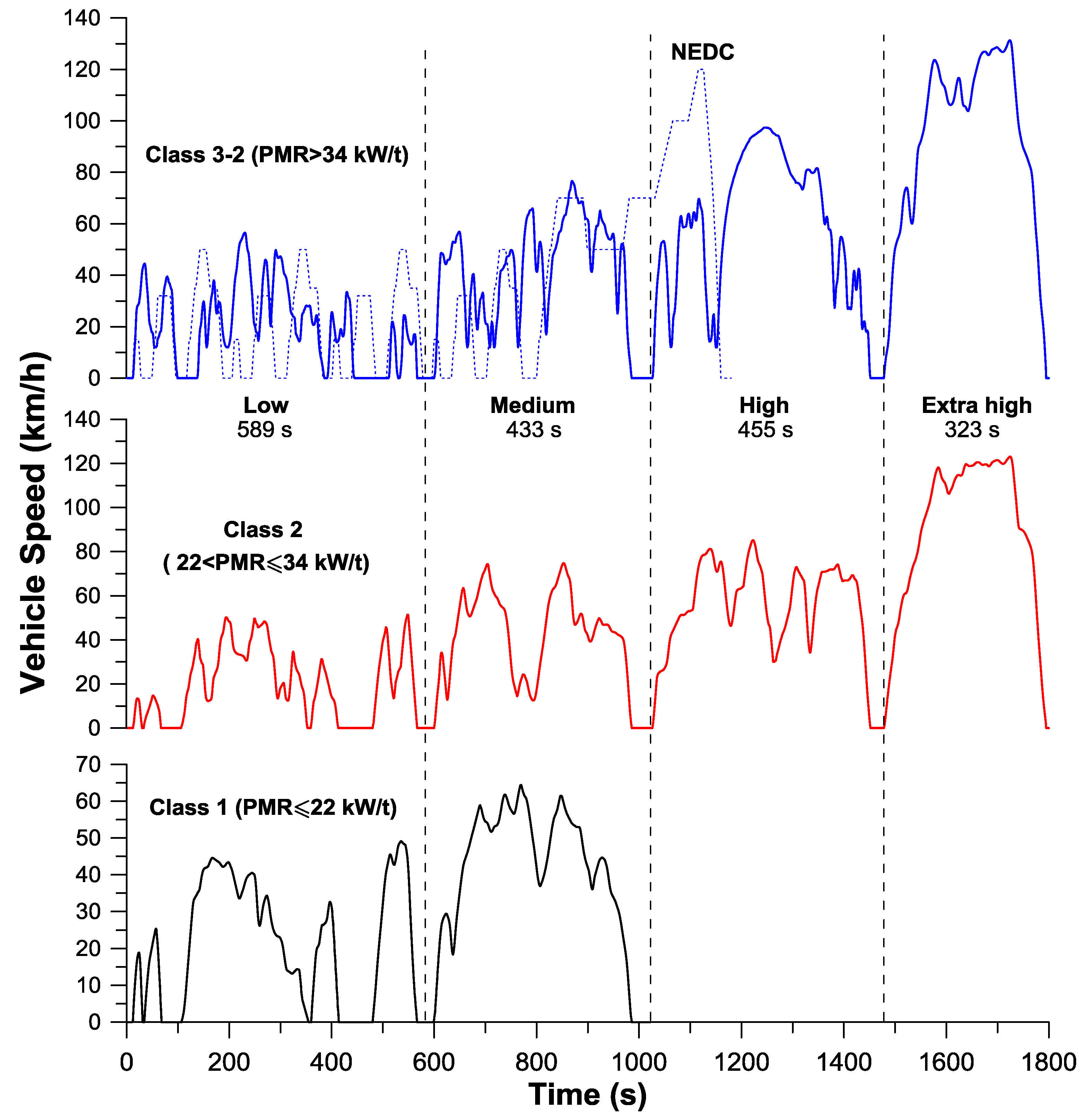This is going to be the worldwide harmonized light-duty vehicles test cycle WLTC, together with the corresponding test procedure WLTP [24]. The WLTC is actually a suite of cycles, with different speed/time schedules depending on the tested vehicle’s power to mass ratio (PMR); the corresponding speed/time traces for the three classes are illustrated in Figure 1. Particularly for Europe, the concerned class is mostly Class 3-2, which is appropriate for the power to mass ratio of the majority of European cars.

Duration of the WLTC is 1800 s, which was believed to represent an acceptable compromise between statistical representativeness on the one hand and test feasibility in the laboratory on the other. The duration of each cycle segment was set in a way that reflected the mileage distribution among the phases, thus no weighting factors were necessary for the final result. Specifically, the low segment lasts 589 s (five micro-trips), the medium 433 s (only one micro-trip), the high 455 s (one micro-trip), and the extra high 323 s (one micro-trip). 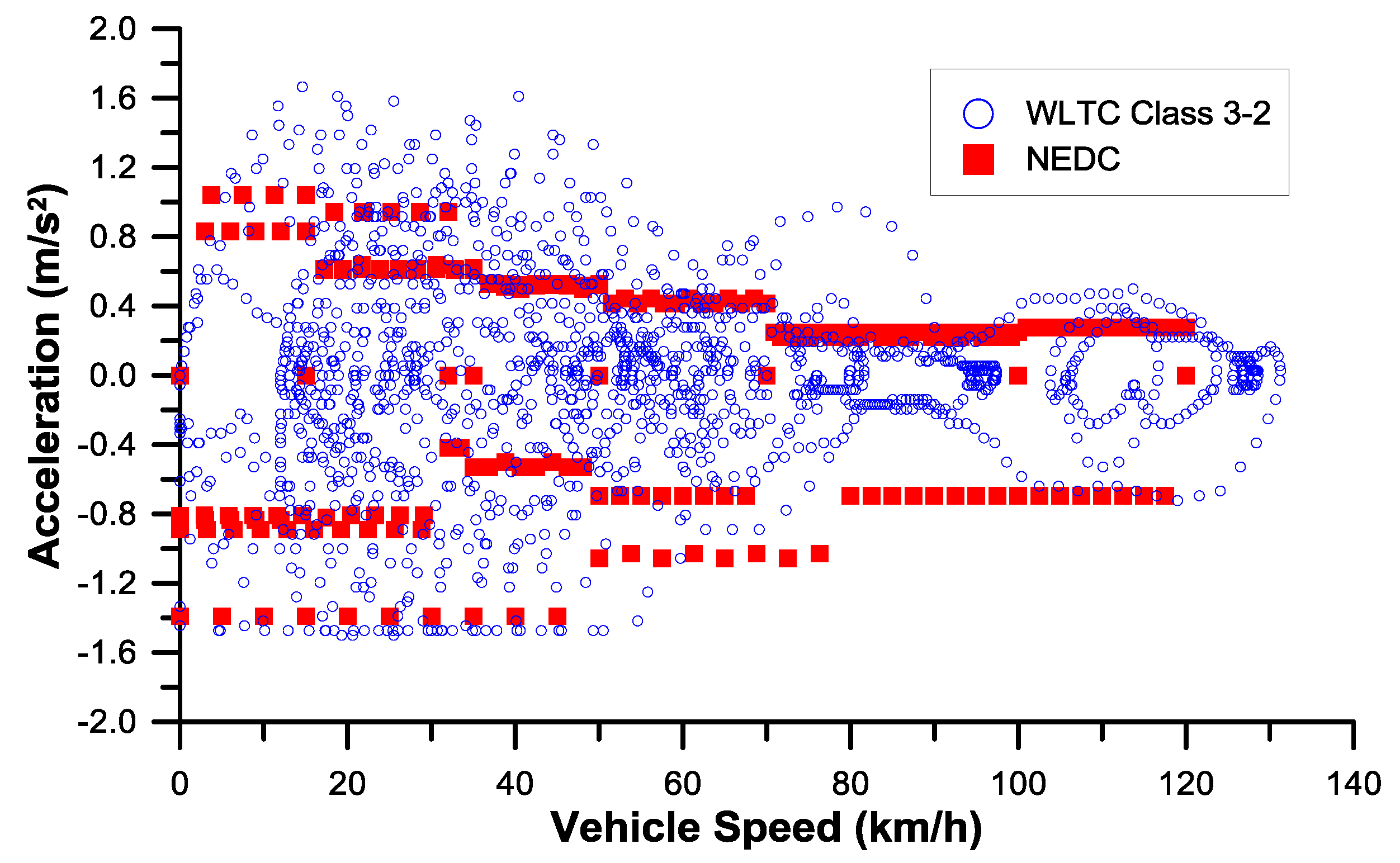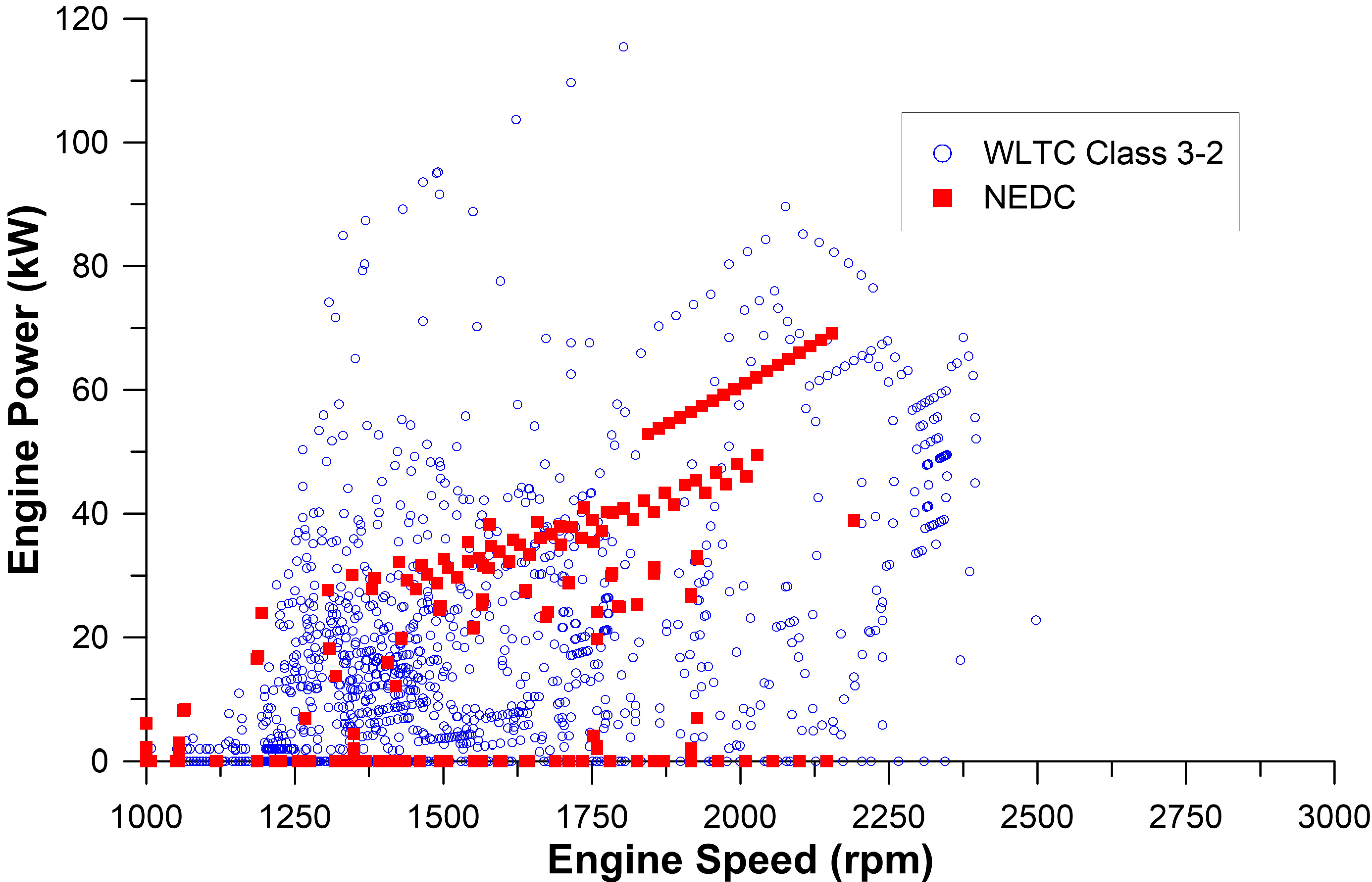Figure 2 demonstrates the speed/acceleration distribution for Class 3-2 which is under study in this work; the corresponding NEDC speed/acceleration points are also provided in this figure needed for the comparison that will be presented later in the text. Further,

Table 1. Summary of technical specifications of the WLTC Class 3-2 [4].

Segment	Duration (s)	Distance (m)	Max. Speed (km/h)	Average Speed (km/h)	Max. Acceleration (m/s2)	Idling Time (%)	Relative Positive Accel. (RPA) (m/s2)
Low	589	3094	56.5	18.9	1.61	24.4	0.219
Medium	433	4756	76.6	39.5	1.61	10.9	0.206
High	455	7162	97.4	56.7	1.67	6.4	0.138
Extra high	323	8254	131.3	92.0	1.06	1.9	0.127
WLTC 3-2	1800	23,266	131.2	46.5	1.67	12.6	0.159

lists the main technical specifications of each segment and of the entire WLTC that will be useful for discussion later in the text.

Further, the corresponding UNECE Global Technical Regulation (GTR) No. 15 provides gear selection and shift point determination (the gear shift strategy being vehicle dependent and not fixed as is the case with the European NEDC), reference fuels, road-load and dynamometer setting, test equipment such as analyzers and their calibrations, and test procedure and conditions to be followed during the certification [24].

Comparison between the WLTC and the NEDC

Since the WLTC will replace from September 2017 the NEDC in the European Union for the certification of new passenger cars and light-duty trucks, the following paragraphs provide a direct comparison between the two cycles as regards their technical specifications (comparison of the respective engine emission results will be presented in Section 4.2).

The NEDC is quite simple to drive and thus easily repeatable as Figure 1 demonstrates. However, as already argued, it does not account for real driving behavior in actual traffic, containing many constant-speed and constant-acceleration segments. In fact, from several observations it has been shown that in Europe the gap between fuel consumption and emissions experienced by the vehicle on the road and those measured at type approval is higher compared to other areas of the world [1]. The overall simplistic pattern of the NEDC and the exact gear-shift schedule make it easy for the manufacturers to implement cycle-beating techniques. Moreover, since it is only run once, cold started, its short distance might over-emphasize cold-starting emission effects. Oddly for its outdated structure, the encountered speeds are relatively high, at least compared to its Japanese (JC08 and earlier J10-15) and U.S. (FTP-75 and HFET) counterparts.

The WLTC, compared to the NEDC, lasts longer and covers more than double distance (see

Table 2. Comparison of the technical specifications between the WLTC and the NEDC driving schedules.

Specification	NEDC	WLTC 3-2	Difference (from NEDC Values)	Effect
Duration (s)	1180	1800	+53%	Lower influence of cold-start emissions
Distance (m)	11,000	23,266	+112%
Average speed (km/h)	33.6	46.5	+38%	Most probably, better fuel efficiency
Maximum speed (km/h)	120	131.3	+9%	More realistic of today’s driving habits
Idling time (%)	23.7	12.6	−47%	Lower influence of start-stop systems
Cruising (%)	39.6	3.7	−91%	More transient, hence higher, pollutant and CO2 emissions
Transient time (%)	36.7	83.7	+128%
Maximum acceleration (m/s2)	1.04	1.67	+60.5%
Average acceleration (m/s2)	0.594	0.406	−31%
RPA (m/s2)	0.116	0.159	+37%

that compares some important technical attributes of the two cycles). This is then reflected into cold-start emission effects being relatively lower. From a purely measurement/experimental point of view, the longer duration of the WLTC poses a burden on the test-bed capacity (e.g., sampling bags). Furthermore, the WLTC has higher maximum, average, and driving speeds, and almost half the idling period (although the single stop with the longest duration is 66 s in the WLTC and only 27 s in the NEDC).

3. Methodology

3.1. Description of the Experimental Procedure

Figure 3 illustrates the experimental set-up developed, which was mostly transient oriented. In particular, for the (continuous) measurement of NO emissions, the ultra-fast response analyzer CLD500 by Cambustion Ltd. was employed. This is a chemiluminescent detector used for measuring NO and NO_x concentration in the exhaust gas with a 90%–10% response time of approximately 2 ms for NO and 10 ms for NO_x [25]. The exhaust gas opacity was measured (continuously) with the AVL-439 partial flow opacimeter. In this device, the sample flows continuously through the opacimeter with an analog output rate of 50 Hz, hence it is appropriate for transient measurements. The location of each measuring device on the experimental test bed installation is given in Figure 3. All the signals from the measuring devices and instruments were fed to the input of the data acquisition module that was connected to a PC via USB interface; details on the experimental set-up are available in [26].

Table 3. Data of the engine and vehicle used for the analysis.

Engine
Engine type	Four-stroke, in-line, six-cylinder, turbocharged, after-cooled, DI diesel engine
Bore/Stroke	97.5 mm/133 mm
Compression ratio	18:1
Maximum power	177 kW @ 2600 rpm
Moment of inertia	0.87 kg m2
Vehicle
Gross vehicle weight	3.5 tn
Frontal area	3 m2
Aerodynamic resistance coefficient	0.38
Gear ratios	5.78; 2.7; 1.9; 1.25; 1.0; 0.9

provides the main technical characteristics of the engine under study; furthermore, it provides the data for a typical (hypothetical) vehicle the engine is installed in, needed for the computational analysis of Section 4. It should be noted that the current engine is not targeted to passenger cars but to medium-duty vehicles such as large vans or even small trucks. The vehicle specifications in Table 3, therefore, correspond to the largest vans available in the European market.

Initially, a detailed experimental investigation of the engine was performed at steady-state conditions to derive its mapping with regard to performance and emissions. Afterwards, a variety of transient schedules was conducted—i.e., discrete speed and load changes—so as to be able to perform the emission overshoot analysis that will be described in Section 3.4.

3.2. Description of the Computational Procedure

Figure 4 illustrates schematically the computational procedure for the estimation of the performance and emissions during the driving cycle. The analysis is based on the previously described steady-state and transient experimental investigation of the engine in hand. Based on the initial measurements at steady-state conditions, a quasi-steady mapping of the engine performance and (engine-out) emissions was initially accomplished. More specifically, for each engine rotational speed, a fourth order polynomial was formulated for every interesting property with respect to the engine torque [10]. For the current investigation, the engine parameters under consideration are nitric oxide (NO), soot, and fueling (hence CO₂ emissions), although any other property (e.g., NO_x, carbon monoxide CO, hydrocarbons HC, particulates, noise, etc.) can be easily formulated with the above-mentioned procedure. NO and soot emissions were chosen for the present analysis owing to the fact that a detailed set of experimental measurements for these two pollutants was available under both steady-state and transient conditions. In particular, NO forms the biggest part of NO_x emissions from diesel engines, whereas soot is studied here as a surrogate to particulate matter, which is very difficult to measure instantaneously.

Based on the block diagram of Figure 4, at each “second” in the cycle:

(a)

From the vehicle speed, which is the input in this study, the actual engine speed and torque are calculated employing the drive-train analysis that will be presented in Section 3.3;

(b)

An interpolation is performed from the digitized engine map in order to assess the corresponding steady-state emissions and fueling at the exact engine speed and load operating point;

(c)

Correction coefficients detailed in Section 3.4 are then applied to the steady-state emissions of the previous step in order to evaluate the “real” transient emissions; the coefficients are based on the specific transient condition (speed and/or load increase) experienced by the engine.

Finally, integration of the instantaneous results is performed over the whole cycle providing the overall emissions and fuel consumption.

3.3. Drive-Train Analysis

Figure 5 illustrates a typical engine power-train configuration, consisting of the six-cylinder engine, (manual) transmission, final drive-train, and wheels. Application of Newton’s second law of motion on the crankshaft axis gives [27,28]

$${\mathsf{\tau }}_{\mathrm{e}}-\frac{{\mathsf{\tau }}_{\mathrm{L}}}{{\mathsf{\eta }}_{\mathrm{g}}}={\mathsf{\tau }}_{\mathrm{A}}={\mathrm{G}}_{\mathrm{V}}\frac{\mathrm{d}\mathsf{\omega }}{\mathrm{dt}},$$

(1a)

In Equation (1a), the engine torque ${\mathsf{\tau }}_{\mathrm{e}}$ is absorbed by the resistances to the vehicle’s motion ${\mathsf{\tau }}_{\mathrm{L}}$ (Equations (4)–(7)) or by the vehicle acceleration ${\mathrm{G}}_{\mathrm{V}}\frac{\mathrm{d}\mathsf{\omega }}{\mathrm{dt}}$, with G_V the vehicle inertia defined in Equation (8) later in the text, and $\mathsf{\omega }$ the engine angular velocity. Further, we assume that the various gears (clutch, gearbox, back-axle) absorb another portion of the engine brake torque owing to viscous and mechanical losses; the latter are defined through total gear efficiency η_g, which for the present study assumes the (typical) value of 0.96 [28]. The above relation holds true when the clutch is engaged, that is speed N_C (i.e., the input speed to the power-train [27]) equals engine rotational speed N. For the case where no gear is engaged (N_C ≠ N), Equation (1a) is transformed into

$$\frac{{\mathsf{\tau }}_{\mathrm{L}}}{{\mathsf{\eta }}_{\mathrm{g}}}+{\mathrm{G}}_{\mathrm{V}}\frac{\mathrm{d}\mathsf{\omega }}{\mathrm{dt}}=0,$$

(1b)

Furthermore, and with reference to Figure 5, N_S is the speed of the propeller shaft, N_A the wheel rotational speed, i_b the back-axle ratio, and i_g the engaged ratio in the gearbox (Table 2); the latter ratios are defined as follows

$${\mathrm{i}}_{\mathrm{g}}=\frac{{\mathrm{N}}_{\mathrm{C}}}{{\mathrm{N}}_{\mathrm{S}}}, \mathrm{and} {\mathrm{i}}_{\mathrm{b}}=\frac{{\mathrm{N}}_{\mathrm{S}}}{{\mathrm{N}}_{\mathrm{A}}}$$

(2)

The instantaneous speed reached by the vehicle is then given by

$$\mathrm{V}(\mathrm{km}/\mathrm{h})=2 \mathsf{\pi } {\mathrm{r}}_{\mathrm{wheel}}\frac{{\mathrm{N}}_{\mathrm{C}}(\mathrm{rpm})}{{\mathrm{i}}_{\mathrm{b}} {\mathrm{i}}_{\mathrm{g}}}\cdot 60\times {10}^{-3}$$

(3)

The three resistance forces experienced by a vehicle when traveling on the road are the aerodynamic-resistance force F_a, the velocity-dependent rolling resistance force F_r, and the grade-dependent force F_gr. Total traction force F_tr is given by

$${\mathrm{F}}_{\mathrm{tr}}={\mathrm{F}}_{\mathrm{a}}+{\mathrm{F}}_{\mathrm{r}}+{\mathrm{F}}_{\mathrm{gr}}$$

(4)

The grade term, however, is not considered here since both studied driving cycles assume straight roads without grade effects. The other two terms in Equation (4) are defined as follows [28]:

The aerodynamic force F_a is given by

$${\mathrm{F}}_{\mathrm{a}}=\frac{1}{2} {\mathsf{\rho }}_{\mathsf{\alpha }} {\mathrm{c}}_{\mathrm{d}} {\mathrm{A}}_{\mathrm{f}} {\mathrm{V}}^2$$

(5)

with A_f the vehicle frontal area, ρ_α the air density and c_d the vehicle aerodynamic resistance (drag) coefficient.

The rolling resistance force F_r is given by

$${\mathrm{F}}_{\mathrm{r}}={\mathrm{m}}_{\mathrm{V}}\left(\mathrm{f}+{\mathrm{c}}_{\mathrm{tr}}\mathrm{V}\right)$$

(6)

The latter incorporates the tire rolling resistance (through friction coefficient f), tire deformation, friction in the wheel bearing and any other friction elements that are a function of the vehicle motion (defined through vehicle speed V); m_V is the loaded mass of the vehicle (Table 2).

For the resistance (traction) torque, it holds that ${\mathsf{\tau }}_{\mathrm{tr}}={\mathrm{F}}_{\mathrm{tr}} {\mathrm{r}}_{\mathrm{wheel}}$. This traction torque τ_tr needs to be reduced to the crankshaft axis in order to be used in Equation (1)

$${\mathsf{\tau }}_{\mathrm{L}}={\mathsf{\tau }}_{\mathrm{tr}} \left(\frac{1}{{\mathrm{i}}_{\mathrm{b}}}\right) \left(\frac{1}{{\mathrm{i}}_{\mathrm{g}}}\right)$$

(7)

Finally, the vehicle’s total moment of inertia G_V, reduced to the crankshaft axis, is given by

$${\mathrm{G}}_{\mathrm{V}}={\mathrm{m}}_{\mathrm{V}} {\mathrm{r}}_{\mathrm{wheel}}^2{\left(\frac{1}{{\mathrm{i}}_{\mathrm{b}}}\right)}^2{\left(\frac{1}{{\mathrm{i}}_{\mathrm{g}}}\right)}^2+{\mathrm{G}}_{\mathrm{e}}+{\mathrm{G}}_{\mathrm{other}}$$

(8)

with G_e the engine moment of inertia including the flywheel (0.87 kg m²) and G_other the inertia of wheels, tires, etc. (when reduced to the crankshaft axis) which equals 1.12 kg m².

Using the previous relations, engine acceleration dω/dt from Equation (1a) is finally given by

$$\mathsf{\epsilon }=\frac{\mathrm{d}\mathsf{\omega }}{\mathrm{dt}}=\frac{{\mathsf{\tau }}_{\mathrm{e}}-\frac{\left(\frac{1}{2} {\mathsf{\rho }}_{\mathsf{\alpha }} {\mathrm{c}}_{\mathrm{d}} {\mathrm{A}}_{\mathrm{f}}{\mathrm{V}}^2+{\mathrm{m}}_{\mathrm{V}}\left(\mathrm{f}+{\mathrm{c}}_{\mathrm{tr}}\mathrm{V}\right)\right) \left(\frac{1}{{\mathrm{i}}_{\mathrm{b}} {\mathrm{i}}_{\mathrm{g}}}\right) {\mathrm{r}}_{\mathrm{wheel}}}{{\mathsf{\eta }}_{\mathrm{g}}}}{{\mathrm{m}}_{\mathrm{V}} {\mathrm{r}}_{\mathrm{wheel}}^2{\left(\frac{1}{{\mathrm{i}}_{\mathrm{b}}}\right)}^2{\left(\frac{1}{{\mathrm{i}}_{\mathrm{g}}}\right)}^2+{\mathrm{G}}_{\mathrm{e}}+{\mathrm{G}}_{\mathrm{other}}}$$

(9)

Application of the above-described drive-train model is necessary so as to convert the vehicle speed vs. time data of the cycle from Figure 1, into engine speed/engine torque vs. time points. After that, the simulation analysis described in Section 3.2 can be applied for the initial (quasi-steady) estimation of exhaust emissions, before the transient discrepancy coefficients are applied, as described in the following section. It should be pointed out that the vehicle motion model developed incorporates the effect of the equivalent rotating mass’ inertia (engine, driveshaft, wheels) as well as tire slip effects.

3.4. Discrepancies during Transient Operation

During steady-state operation, engine speed and fueling, and by extension all the other engine and turbocharger properties, remain essentially constant. Under transient conditions, however, either after a speed or load change, both the engine speed and the fuel supply change continuously. Consequently, the available exhaust gas energy varies, affecting the turbine enthalpy drop and, through the turbocharger shaft torque balance, the boost pressure and the air-supply to the engine cylinders are influenced too. However, due to various dynamic, thermal, and fluid delays—mainly originating in the turbocharger moment of inertia—combustion air-supply is delayed compared to fueling, adversely affecting torque build-up and vehicle drivability. The low air–fuel equivalence ratios experienced after a speed or load increase transient event considerably enhance the formation of soot (to values far beyond the acceptable steady-state levels); the latter is experienced as black smoke coming out of the exhaust pipes of older technology vehicles with no after-treatment control. Further, the occurrence of high combustion temperatures (owing to close to stoichiometric mixtures, where gas temperatures peak [29]), favor the production of NO_x [2,4]. The above described phenomena, which are more serious the lower the initial load or speed of the individual transient event, are encountered at each acceleration throughout a driving cycle.

In order to account for the serious transient discrepancies, correction coefficients are applied to the quasi-steady emissions, based on various experimental tests at transient conditions performed for the particular engine. Although vehicular engines experience steep accelerations, they usually undergo rather soft load changes [3,4]. Hence, for the current analysis, it is contended that mainly the speed increases contribute to the transient emission overshoots throughout the cycle. The transient emission correction procedure is based on the following two well-established facts [3,4,26,30]:

(a)

The transient emission overshoot is higher at lower initial speeds or loads (a lower initial turbocharger boost pressure results in “harsher” turbocharger lag);

(b)

The transient emission overshoot is higher at steeper accelerations.

In order to assess the emission overshoot experienced by the engine during transients compared to the respective quasi-steady conditions, various individual accelerations, such as the ones experienced during a driving cycle, were conducted from various initial speeds and loads. From these, it was revealed that, for the current engine configuration, the transient emissions increase could be satisfactorily accounted for by applying the following equation

$$\text{Transient Emissions} (\mathrm{t})=\text{Steady-steady Emissions} (\mathrm{t})\times \left\{1+{\mathrm{c}}_{\mathrm{speed}}\cdot {\left(\text{relative speed change}\right)}_{\mathrm{t}-1}^{\mathrm{t}}\right\}$$

(10)

In other words, correction coefficient c_speed increases the instantaneous quasi-steady emissions at each operating point (second) in the cycle based on the acceleration encountered from the previous to the current operating point. It should be pointed out that the c_speed coefficients are different for each investigated pollutant. Further, the c_speed coefficients do not assume the same value throughout the whole engine operating range. In order to estimate their values (and at the same time incorporate the effect of the above-mentioned points “a” and “b” in our analysis), the possible accelerations have been divided into three ranges. The first range comprises the accelerations commencing from idling or very low engine speed (1000–1400 rpm). This is the most difficult scenario for the engine since the turbocharger operates at or near zero boost pressure and the turbocharger lag is more pronounced during the transient event, increasing accordingly the (engine-out) emissions overshoot. Details about the results of this procedure and the (linear) best-fit curve for the formulation of the acceleration-dependent term in Equation (10) are provided in Figure 6. This figure depicts the emission overshoot for the case of speed increases commencing from an initial engine speed of 1200 rpm up to the final steady-state speed, compared to the respective quasi-steady emissions.

The second range comprises the accelerations commencing from an initial engine speed of 1401–1800 rpm, and the third range comprises the accelerations commencing from an initial speed higher than 1800 rpm, where the turbocharger lag effects are milder, hence the value of the c_speed coefficient smaller. For each one of the three above-mentioned speed ranges, three values of the c_speed coefficient were derived for each pollutant based on the initial engine load of each acceleration (lower than 30%, 31%–60% and higher than 60% of the engine’s full load). By doing so, engine load increase effects were accounted for too in the transient correction procedure.

Overall, we have derived nine values of the coefficients c_speed for soot emissions and nine values for NO emissions, ranging from 1.1 to 4.0 for NO, and from 25 to 120 for soot, as demonstrated in

Table 4. Values for the c_speed coefficients used in the analysis for NO and soot.

Speed Range (rpm)	NO Coefficients	Soot Coefficients
1000–1400	4.0 (load change 0%–30%)	120 (load change 0%–30%)
	3.0 (load change 31%–60%)	85 (load change 31%–60%)
	1.6 (load change > 60%)	50 (load change > 60%)
1401–1800	3.2 (load change 0%–30%)	100 (load change 0%–30%)
	2.0 (load change 31%–60%)	70 (load change 31%–60%)
	1.2 (load change > 60%)	40 (load change > 60%)
>1800	2.0 (load change 0%–30%)	60 (load change 0%–30%)
	1.2 (load change 31%–60%)	36 (load change 31%–60%)
	1.1 (load change > 60%)	25 (load change > 60%)

. These values were derived from the experimental study on the current engine and cannot be assumed to apply to other engines; in general, the exact values depend on the technology and tuning of each engine, e.g., possible internal measures, injection timing strategy, etc.

The following important assumption is also valid for the analysis that follows: cold start emissions are ignored (no experimental data was available)—instead the engine is assumed to be in fully warmed-up conditions from the beginning of the cycle. Ignoring the cold start emissions influences the instantaneous and total emission results but this holds particularly true for the CO and HC emissions, which are not considered in this study. On the other hand, engine-out NO (and NO_x) emissions during cold starting for the present engine are rather low, owing to the low gas temperatures involved, and may actually be overestimated by the present methodology [2,4,26,31].

4. Results and Discussion

4.1. WLTC Results

Application of the experimental/simulation procedure outlined in Figure 4 is demonstrated in Figure 7, Figure 8 and Figure 9 regarding performance and emission results from the turbocharged diesel-powered vehicle, the technical details of which were given in Table 3. More specifically, Figure 7 focuses on the vehicle parameters (acceleration, gear, resistance forces), Figure 8 on the engine parameters (speed, power, torque, fueling), and Figure 9 on the development of engine-out emissions (NO, soot, and CO₂).

Notice in Figure 7 the strong influence of vehicle speed on the resistance forces development. Aerodynamic resistance force follows the vehicle speed pattern according to Equation (5), with its rolling resistance counterpart possessing both a constant and a speed-dependent term according to Equation (6). During the urban part of the cycle (0–1022 s), where the vehicle speeds are maintained at low to medium levels, the rolling resistance term prevails over the aerodynamic one (upper sub-diagram of Figure 7). During motorway driving, on the other hand, the aerodynamic force assumes much higher values, backed up by the rather high vehicle frontal area and the much smaller dependence of rolling resistance on vehicle speed. As regards the vehicle acceleration profile, this is particularly dense during the WLTC, compared with the NEDC, the pattern of which is also provided in Figure 7 for comparison purposes. This is not surprising since the WLTC is a true transient cycle derived from actual measurements on the road in contrast to the modal NEDC (cf. Figure 2).

Based on Equation (9), the lower the engaged gear (this results in high i_g in Table 3), e.g., during the urban parts of the cycle, the smaller the total vehicle moment of inertia from Equation (8), ultimately leading to higher acceleration values in Figure 7 [27] (emissions too, as will be discussed later in the text). On the other hand, the higher the engaged gear (hence the lower the respective gear ratio), the higher the vehicle speed and the lower the accelerations in Figure 7 (e.g., the 1200–1300s segment in the cycle) owing to now higher vehicle inertia.

Figure 8 focuses on the development of some interesting engine parameters—namely speed, torque, power and fuel consumption. Perhaps the most important finding from Figure 8 is that the engine speed development is closely patterned after the vehicle acceleration. The development of torque, power, and fueling follows a similar manner throughout the cycle, as all three parameters are inter-related to engine loading. Following the fundamental vehicle analysis of Section 3.3, during the urban segments in the cycle, loading is mainly determined by the vehicle acceleration, as during these parts the absolute vehicle speeds are low but the transient events are both frequent and steep. During the highway segments, on the other hand (small vehicle acceleration values), it is the increased vehicle speed that mostly influences the engine loading (though the aerodynamic resistance force), hence determines the values for torque, power, and fuel consumption. Unsurprisingly, at each acceleration in the cycle, fueling peaks at high values owing to the power needed to overcome the vehicle inertia and the various losses in the transmission system.

Figure 9 focuses on the instantaneous and cumulative engine-out exhaust emissions—namely NO, soot, and CO₂. In general, the points where the most abrupt accelerations are experienced lead also to a considerable overshoot in emissions. Net soot production (fueling as well in Figure 8, hence CO₂ emissions in Figure 9) is mainly dependent on engine load. With increasing load—e.g., during each acceleration in the cycle—more fuel is injected into the cylinders, increasing the temperatures in the fuel-rich zones; at the same time, the duration of diffusion combustion is longer favoring soot formation. On the other hand, two notable soot oxidation contributors, i.e., the remaining time after combustion as well as the availability of oxygen, decrease; thus, the production of soot is favored [2]. During the accelerations in the cycle, the above mechanism is remarkably enhanced by the locally very high values of fuel–air ratios experienced during turbocharger lag. For the overshoot in soot emissions observed therefore in Figure 9 after each acceleration, the main cause is the instantaneous lack of air due to turbocharger lag, further aided by the initial sharp increase in ignition delay during the early thermodynamic cycles of each individual transient event [30,32].

For NO emissions, it is again the lag between increased fueling and the response of the air-supply system that is responsible for the overshoot in emissions. Since the main parameter affecting NO formation is the burned gas temperatures, locally high temperatures, due to close to stoichiometric air–fuel mixtures, increase NO emissions during the turbocharger lag thermodynamic cycles. It should be pointed out however that the relative NO increase (overshoot) is much lower than its soot counterpart, i.e., after each acceleration in the cycle, transient soot peaks/”jumps” way more than NO with respect to the quasi-steady conditions at the previous second in the cycle (cf. Table 4). This is due to the fact that, for the production of NO, there are two contributing parameters: high temperatures and oxygen availability. During the turbocharger lag phase at the onset of each acceleration in the cycle, soot peaks owing to lower than stoichiometric conditions. During these phases, and as long as lambda is lower than unity, the availability of air is limited, hence the overshoot in NO emissions not so pronounced. A closer look at the instantaneous NO and soot traces in Figure 9 also confirms the previously mentioned well established fact that the turbocharger lag discrepancies are more prominent the lower the initial engine (and in this case, vehicle) speeds and the lower the engaged gears. The most pronounced overshoots in both soot and NO are observed at t = 1032 s, where the highest acceleration from standstill is also experienced.

Following engineering intuition and basic combustion theory, the CO₂ overshoots in Figure 9 are patterned exactly after the fueling ones in Figure 8.

Overall, the distance-related engine-out emissions for each cycle segment are summarized in

Table 5. Breakdown of distance-related engine-out emissions and fuel consumption for the various segments of the WLTC.

Segment	Duration (s)	Distance (km)	Micro-Trips	Soot (g/km)	NO (g/km)	Fueling (L/100km)	CO2 (g/km)
Low	589	3094	5	0.214	13.173	8.77	330.28
Medium	433	4756	1	0.086	6.935	6.93	260.87
High	455	7162	1	0.062	5.883	6.08	229.01
Extra high	323	8254	1	0.018	4.010	8.00	301.10
Entire cycle	1800	23,266	7	0.069	6.403	7.29	274.57

.

Clearly, the first segment (urban driving with low speeds) is responsible for the biggest contribution in emissions (g/km), particularly soot, which is primarily influenced by the abrupt accelerations (highest values of c_speed coefficient). This is due to the fact that both average and maximum vehicle acceleration assume higher values during the low (and medium) segment compared to the high and extra high. Furthermore, the low-segment of the WLTC has five micro-trips (compared to only one for each of the other three segments). This means that the percentage of (harsh) accelerations from zero loading is much higher, contributing accordingly to the amount of emitted pollutants. It is worth remembering at this point that the number of stops per km is a typical cycle metric associated with exhaust emissions, particularly from turbocharged diesel engines [1]. Furthermore, the relative positive acceleration (RPA)—another well-established metric of the cycle’s aggressiveness (Table 1)—is greater than 0.20 during the first two cycle segments compared with values of the order of 0.12–0.13 during the high-speed parts of the cycle.

4.2. WLTC vs. NEDC Results

Figure 2 compared the speed/acceleration distribution between the WLTC and the NEDC. The much broader speed/acceleration range of the WLTC confirms the considerable progress over the current NEDC in terms of simulated real-world driving behavior. For approximately 84% of the time during the WLTC, the vehicle operates in transient conditions (accelerating or decelerating), in contrast to only 37% during the NEDC (Table 2). Similarly, cruising time is almost absent during the WLTC, and the RPA is much higher. These are expected to result in higher engine-out pollutant emissions, and higher CO₂. It should be pointed out again that the comparison between the two cycles performed in this section aims to identify only vehicle speed profile effects and not differences located in the different testing procedure (we are comparing the WLTC with the NEDC, and not the WLTP with the NEDC test procedure). In order to perform this kind of comparison, it is assumed in the next paragraphs that both driving cycle schedules are tested over the same “conditions”—e.g., vehicle test mass, temperature, gear-shift strategy. By doing so, we can eliminate all other test-procedure-related differences and isolate the vehicle speed-profile effects. Of course, for type approval purposes on the chassis-dynamometer, each test schedule is carried out according to the specific test procedure (as outlined in the relevant regulatory documents), and the obtained results should be different from the ones presented here, as the basis for the comparison is not the same (e.g., different gear-shift strategy, vehicle test mass, temperature of the test) [33,34].

For the diesel-powered vehicle under study, Figure 10 compares the covered speed/power region when running on the WLTC and the NEDC. Following the remarks made earlier, the engine operates at a much broader range during the WLTC compared with the rather limited operating points tested during the (modal and highly “repetitive”) NEDC; similar results were reached by Steven [35]. Overall, 78% of the operating points during the NEDC correspond to lower than 3000 rpm engine speed and 82% to lower than 20 kW power in Figure 10; for the WLTC, the respective numbers are much smaller, 55% and 68%. Furthermore, the driving pattern during urban driving is much denser throughout the WLTC. Regarding the specific energy, this is of the order of 30.1 kWh/100km for the WLTC, unsurprisingly higher than the respective value of 28.4 kWh/100 km for the NEDC (

Table 6. WLTC vs. NEDC cumulative results (all emissions are engine-out).

Property	NEDC	WLTC 3-2	Difference (from NEDC Values)
Specific Energy (kWh/100 km)	28.40	30.10	+6%
Soot (g/km)	0.0447	0.0694	+55%
NO (g/km)	5.778	6.403	+10.8%
Fueling (L/100 km)	7.36	7.29	−1%
CO2 (g/km)	277.15	274.57	−1%

).

As regards the pollutant engine-out emission results (Table 6), both soot (55%) and NO (10.8%) were found to be higher during the WLTC. This is not surprising based on the latter’s much harsher profile (see also Table 2). For fueling and CO₂ emissions, on the other hand, the trend was slightly reversed, with the NEDC results (277.15 g/km CO₂; 7.36 L/100 km fuel consumption) found somewhat higher than the WLTC ones (274.57 g/km CO₂ and 7.29 L/100 km fuel consumption). This can be attributed to the fact that, for the engine under study, the overall lower level of the average torque and speed (both significant contributors to fuel consumption) during the NEDC led also to slightly higher fuel consumption. Indicative here is Figure 11 that illustrates the second-by-second engine-out emissions for the two cycles. The much softer accelerations during the NEDC clearly result in smaller overshoots regarding both pollutant emissions and CO₂. Similarly small differences in the CO₂ emissions between the WLTC and the NEDC were reached in [35] when (as is also the case in this work) the same test mass for both cycles was applied to isolate the vehicle speed profile effects. On the other hand, when the whole test procedure is under investigation, and not just the cycle speed profile [18,33], the results may be different, with the vehicles exhibiting higher CO₂ emissions during the WLTP compared to the NEDC.

5. Summary and Conclusions

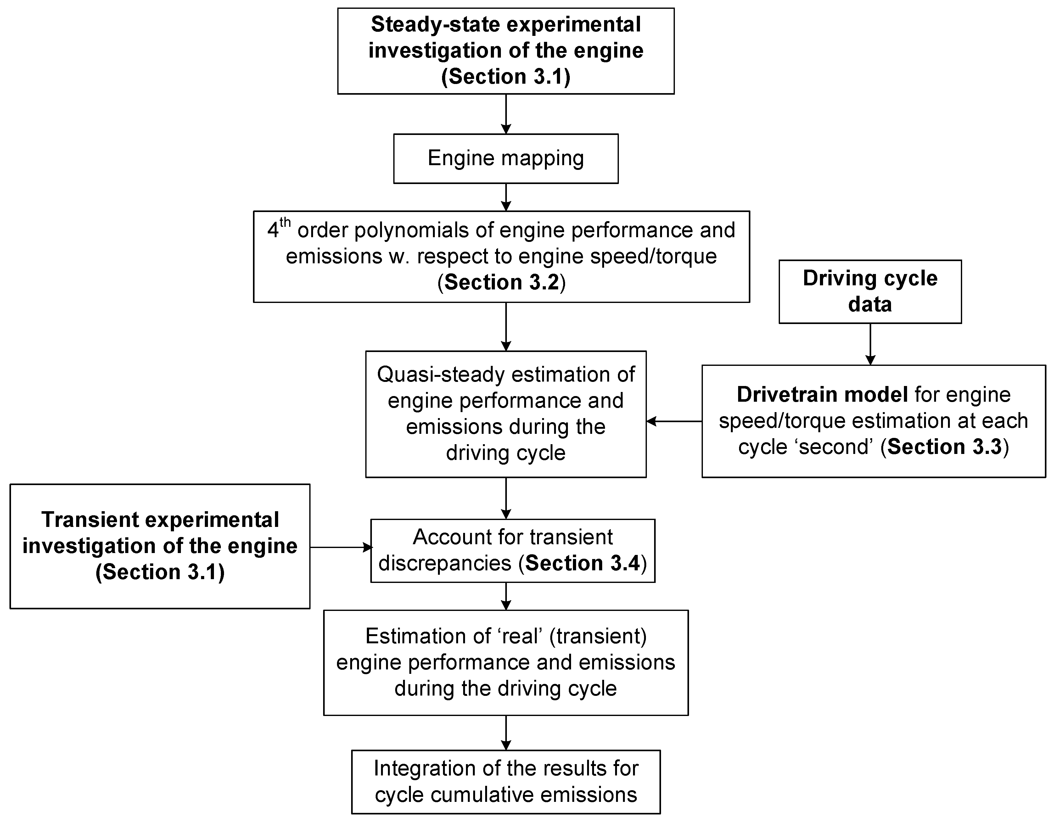
A mapping methodology was proposed and developed to estimate engine and vehicle performance and emissions during the recently developed worldwide WLTC driving cycle. The procedure is based on a steady-state experimental investigation of the engine in hand for the formulation of polynomial expressions of all interesting engine parameters with respect to rotational speed and torque. Correction coefficients were then applied to account for transient discrepancies based on various discrete transient events conducted and analyzed for the engine under study in a specially developed transient test bed. The obvious advantage of the methodology is that neither costly and sophisticated experimental facilities nor huge computational times are required.

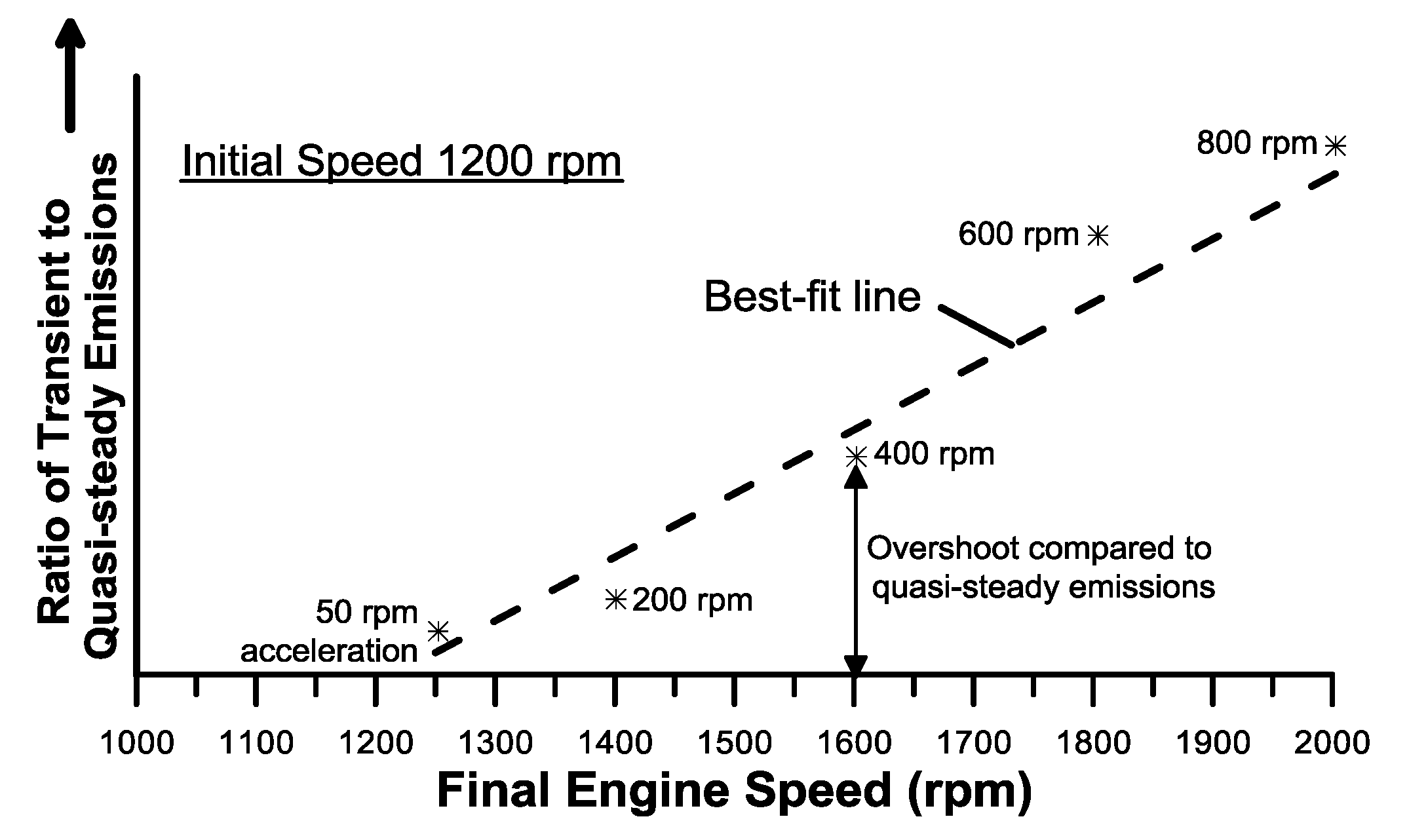
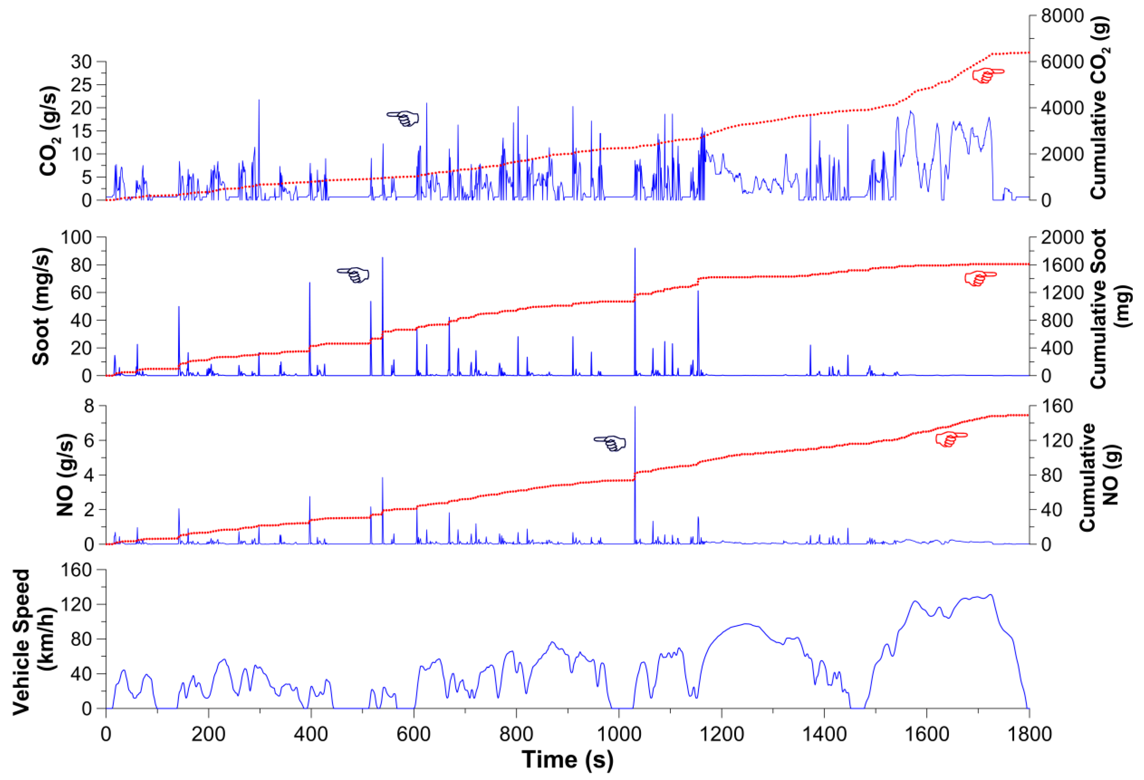
Vehicle speed was identified as the dominant property affecting almost all vehicle parameters and performance in general. A significant differentiation was observed between urban and motorway segments in this respect. As regards the engine, it was the rotational speed fluctuations (initiated by the respective vehicle accelerations) that decisively influenced the engine performance and emissions. At each point in the cycle where an (abrupt) increase in the vehicle speed was experienced, an overshoot in emissions (particularly soot) was noticed; the culprit here was the turbocharger lag.

It was further revealed that the first section (urban driving) of the WLTC is responsible for the biggest amount of emissions (g/km) owing to the most frequent and abrupt accelerations from no load conditions due to its many stops and increased RPA.

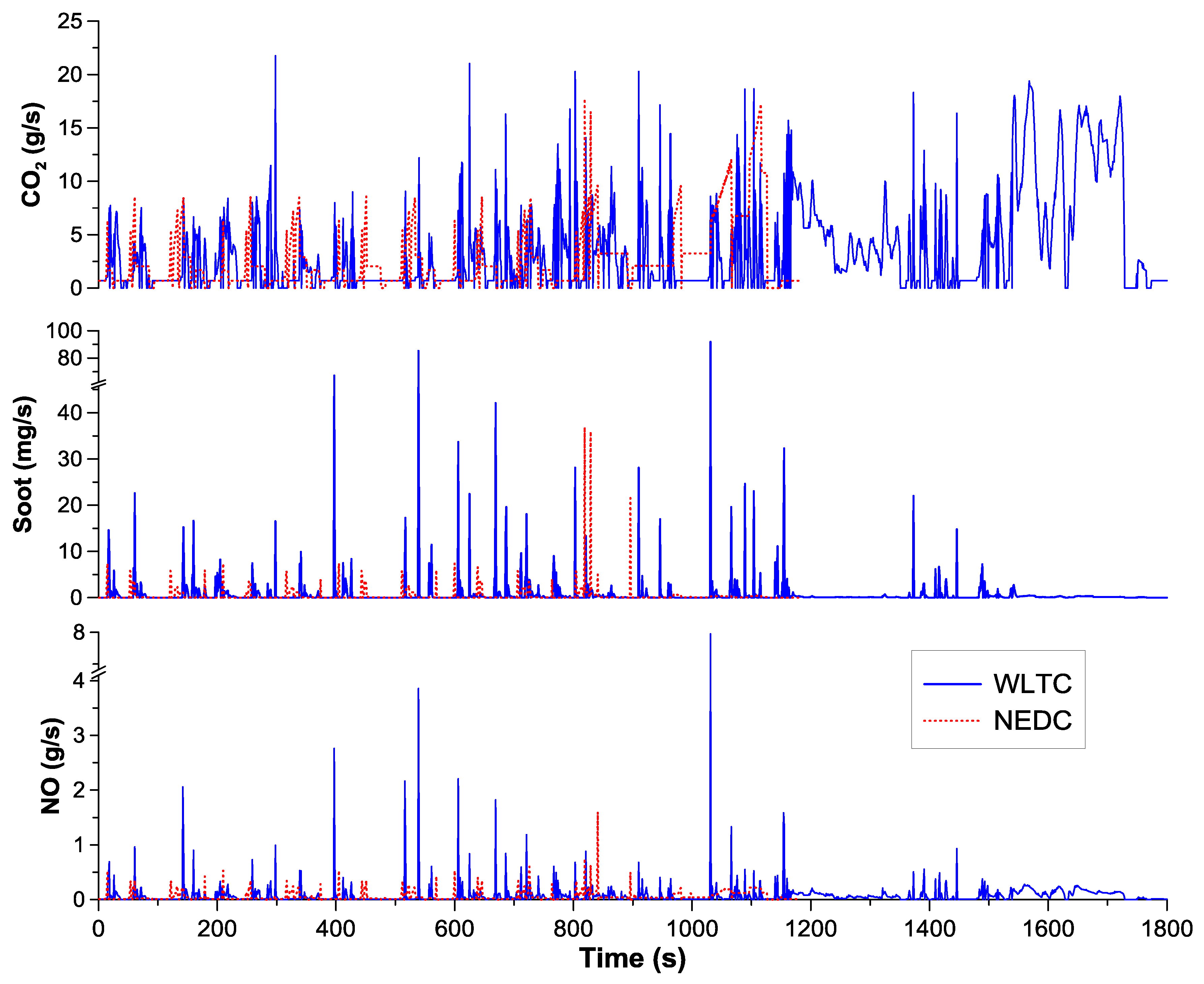
A comparison between the WLTC and the NEDC driving schedules was also performed applying the same vehicle test mass and gear-shift strategy. For the engine/vehicle in hand, it was shown that the WLTC, owing to its truly transient profile (in contrast to the NEDC’s modal form), captures much wider vehicle and engine operating activity, with obvious benefits in terms of real-world driving representativeness. At the same time, the WLTC exhibits higher specific energy and higher pollutant (NO and soot) emissions. On the other hand, owing to the engine operating at a slightly higher load level during the WLTC, the corresponding CO₂ emissions were found somewhat lower compared to the NEDC.

References

1. Giakoumis, E.G. Driving and Engine Cycles; Springer: Cham, Switzerland, 2017. [Google Scholar]
2. Heywood, J.B. Internal Combustion Engine Fundamentals; McGraw-Hill: New York, NY, USA, 1988. [Google Scholar]
3. Watson, N.; Janota, M.S. Turbocharging the Internal Combustion Engine; McMillan: London, UK, 1982. [Google Scholar]
4. Rakopoulos, C.D.; Giakoumis, E.G. Diesel Engine Transient Operation; Springer: London, UK, 2009. [Google Scholar]
5. Gambarotta, A.; Lucchetti, G.; Vaja, I. Real-time modelling of transient operation of turbocharged diesel engine. Proc. Inst. Mech. Eng. D J. Automob. Eng. 2001, 225, 1186–1203. [Google Scholar] [CrossRef]
6. Berglund, S. A Model of Turbocharged Engines as Dynamic Drivetrain Members; SAE Technical Paper 933050; SAE International: New York, NY, USA, 1993. [Google Scholar]
7. Rackmil, C.I.; Blumberg, P.N.; Becker, D.A.; Schuller, R.R.; Garvey, D.C. A dynamic model of a locomotive diesel engine and electrohydraulic governor. J. Eng. Gas Turbines Power 1988, 110, 405–414. [Google Scholar] [CrossRef]
8. Jiang, Q.; Van Gerpen, J.H. Prediction of Diesel Engine Particulate Emission during Transient Cycles; SAE International: New York, NY, USA, 1992. [Google Scholar]
9. Ericson, C.; Westerberg, B.; Egnell, R. Transient Emission Predictions with Quasi Stationary Models; SAE International: New York, NY, USA, 2005. [Google Scholar]
10. Giakoumis, E.G.; Lioutas, S.C. Diesel-engined vehicle nitric oxide and soot emissions during the European light-duty driving cycle using a transient mapping approach. Transp. Res. D 2010, 15, 134–143. [Google Scholar] [CrossRef]
11. Giakoumis, E.G.; Alysandratou, A. Performance and emissions of a heavy-duty truck during the UDDS driving cycle—Simulation analysis. ASCE J. Energy Eng. 2016, 142, E4015011. [Google Scholar] [CrossRef]
12. Kirchen, P.; Obrecht, P.; Boulouchos, K. Soot emission measurements and validation of a mean value soot model for common-rail diesel engines during transient operation. SAE Int. J. Engines 2009, 2, 1663–1678. [Google Scholar] [CrossRef]
13. Roy, S.; Banerjee, R.; Bose, P.K. Performance and exhaust emissions prediction of a CRDI assisted single cylinder diesel engine coupled with EGR using artificial neural network. Appl. Energy 2014, 119, 330–340. [Google Scholar] [CrossRef]
14. Johri, R.; Filipi, Z. Neuro-fuzzy model tree approach to virtual sensing of transient diesel soot and NOx emissions. Int. J. Engine Res. 2014, 15, 918–927. [Google Scholar] [CrossRef]
15. Bishop, J.D.K.; Stettler, M.E.J.; Molden, N.; Boies, A.M. Engine maps of fuel use and emissions from transient driving cycles. Appl. Energy 2016, 183, 202–217. [Google Scholar] [CrossRef]
16. Tutuianu, M.; Bonnel, P.; Ciuffo, B.; Haniu, T.; Ichikawa, N.; Marotta, A.; Pavlovic, J.; Steven, H. Development of the worldwide harmonized light duty test cycle (WLTC) and a possible pathway for its introduction in the European legislation. Transp. Res. D 2015, 40, 61–75. [Google Scholar] [CrossRef]
17. Mock, P.; Kühlwein, J.; Tietge, U.; Franco, V.; Bandivadekar, A.; German, J. The WLTP: How a New Test Procedure for Cars Will Affect Fuel Consumption Values in the EU. ICCT Working Paper 2014-9. 2014. Available online: http://www.theicct.org/wltp-how-new-test-procedure-cars-will-affect-fuel-consumption-values-eu (accessed on 25 November 2016).
18. Favre, C.; Bosteels, D.; May, J. Exhaust Emissions from European Market-Available Passenger Cars Evaluated on Various Drive Cycles; SAE International: New York, NY, USA, 2013. [Google Scholar]
19. Sileghem, L.; Bosteels, D.; May, J.; Favre, C.; Verhelst, S. Analysis of vehicle emission measurements on the new WLTC, the NEDC and the CADC. Transp. Res. D 2014, 32, 70–85. [Google Scholar] [CrossRef] [Green Version]
20. Andersson, J.; May, J.; Favre, C.; Bosteels, D.; De Vries, S.; Heaney, M.; Keenan, M.; Mausell, J. On-Road and Chassis Dynamometer Evaluations of Emissions from Two Euro 6 Diesel Vehicles; SAE International: New York, NY, USA, 2014. [Google Scholar]
21. Marotta, A.; Pavlovic, J.; Ciuffo, B.; Serra, S.; Fontaras, G. Gaseous emissions from light-duty vehicles: Moving from NEDC to the new WLTP test procedure. Environ. Sci. Technol. 2015, 49, 8315–8322. [Google Scholar] [CrossRef] [PubMed]
22. Bielaczyc, P.; Woodburn, J.; Szczotka, A. A Comparison of Carbon Dioxide Exhaust Emissions and Fuel Consumption for Vehicles Tested over the NEDC, FTP-75 and WLTC Chassis Dynamometer Test Cycles; SAE International: New York, NY, USA, 2015. [Google Scholar]
23. Tsokolis, D.; Tsiakmakis, S.; Dimaratos, A.; Fontaras, D.; Pistikopoulos, P.; Ciuffo, B.; Samaras, Z. Fuel consumption and CO2 emissions of passenger cars over the New Worldwide Harmonized Test Protocol. Appl. Energy 2016, 179, 1152–1165. [Google Scholar] [CrossRef]
24. Global Technical Regulation No. 15. Worldwide Harmonized Light Vehicles Test Procedure. Established in the Global Registry on 12 March 2014. Available online: https://www.unece.org/fileadmin/DAM/trans/main/wp29/wp29r-1998agr-rules/ECE-TRANS-180a15e.pdf (accessed on 14 January 2017).
25. Collier, T.; Gregory, D.; Rushton, M.; Hands, T. Investigation into the Performance of an Ultra-Fast Response NO Analyzer Equipped with a NO2 to NO Converter for Gasoline and Diesel Exhaust NOx Measurements; SAE International: New York, NY, USA, 2000. [Google Scholar]
26. Rakopoulos, C.D.; Dimaratos, A.M.; Giakoumis, E.G.; Peckham, M.S. Experimental Assessment of Turbocharged Diesel Engine Transient Emissions during Acceleration, Load Change and Starting; SAE International: New York, NY, USA, 2010. [Google Scholar]
27. Winterbone, D.E.; Benson, R.S.; Mortimer, A.G.; Kenyon, P.; Stotter, A. Transient Response of Turbocharged Diesel Engines; SAE International: New York, NY, USA, 1977. [Google Scholar]
28. Gillespie, T.D. Fundamentals of Vehicle Dynamics; SAE International: Warrendale, PA, USA, 1992. [Google Scholar]
29. Law, C.K. Combustion Physics; Cambridge University Press: Cambridge, UK, 2006. [Google Scholar]
30. Hagena, J.R.; Filipi, Z.S.; Assanis, D.N. Transient Diesel Emissions: Analysis of Engine Operation during a Tip-In; SAE International: New York, NY, USA, 2006. [Google Scholar]
31. Bielaczyc, P.; Merkisz, J.; Pielecha, J. Investigation of Exhaust Emissions from di Diesel Engine during Cold and Warm Start; SAE International: New York, NY, USA, 2001. [Google Scholar]
32. Wijetunge, R.S.; Brace, C.J.; Hawley, J.G.; Vaughan, N.D.; Horrocks, R.W.; Bird, G.L. Dynamic Behavior of a High Speed Direct Injection Diesel Engine; SAE International: New York, NY, USA, 1999. [Google Scholar]
33. Pavlovic, J.; Marotta, A.; Ciuffo, B. CO2 emissions and energy demands of vehicles tested under the NEDC and the new WLTP type approval test procedures. Appl. Energy 2016, 177, 661–670. [Google Scholar] [CrossRef]
34. Dimaratos, A.; Tsokolis, D.; Fontaras, D.; Tsiakmakis, S.; Ciuffo, B.; Samaras, Z. Comparative evaluation of the effect of various technologies on light-duty vehicle CO2 emissions over NEDC and WLTP. Transp. Res. Procedia 2016, 14, 3169–3178. [Google Scholar] [CrossRef]
35. Steven, H. Homologation Test Cycles Worldwide-Status of the WLTP. Green Global NCAP Labelling/Green Scoring Workshop. 30 April 2013. Available online: https://www.iea.org/media/workshops/2013/gfeilabelling/07.08.Homologationtestcyclesworldwide.pdf (accessed on 14 January 2017).
Figure 1. Speed profile of the WLTC driving cycle for Classes 1, 2, and 3-2 (Class 3-1 differs slightly from 3-2, being intended for the special category of k-cars in Japan); discontinuous line along the Class 3-2 graph shows the currently employed in Europe NEDC speed/time trace (PMR: power to mass ratio).
Energies 10 00240 g001
Figure 2. Comparison of the speed/acceleration distribution between the WLTC Class 3-2 and the NEDC.
Energies 10 00240 g002
Figure 3. Illustration of the experimental set-up for steady-state and transient measurements.
Energies 10 00240 g003
Figure 4. Block diagram of the developed methodology.
Energies 10 00240 g004
Figure 5. Illustration of vehicle drivetrain.
Energies 10 00240 g005
Figure 6. Example of transient overshoot for the emissions correction procedure.
Energies 10 00240 g006
Figure 7. Development of vehicle parameters during the WLTC.
Energies 10 00240 g007
Figure 8. Development of engine parameters during the WLTC.
Energies 10 00240 g008
Figure 9. Development of engine-out emissions during the WLTC.
Energies 10 00240 g009
Figure 10. Comparison of the engine speed/power tested points between the WLTC Class 3-2 and the NEDC for the diesel-powered vehicle under study.
Energies 10 00240 g010
Figure 11. Comparison of the second-by-second engine-out emissions between the WLTC Class 3-2 and the NEDC (the NEDC lasts 1180 s and the WLTC 1800 s).
Energies 10 00240 g011