Optimization Models for Islanded Micro-Grids: A Comparative Analysis between Linear Programming and Mixed Integer Programming

Abstract

This paper presents a comparison of optimization methods applied to islanded micro-grids including renewable energy sources, diesel generators and battery energy storage systems. In particular, a comparative analysis between an optimization model based on linear programming and a model based on mixed integer programming has been carried out. The general formulation of these models has been presented and applied to a real case study micro-grid installed in Somalia. The case study is an islanded micro-grid supplying the city of Garowe by means of a hybrid power plant, consisting of diesel generators, photovoltaic systems and batteries. In both models the optimization is based on load demand and renewable energy production forecast. The optimized control of the battery state of charge, of the spinning reserve and diesel generators allows harvesting as much renewable power as possible or to minimize the use of fossil fuels in energy production.

1. Introduction

Islanded micro-grids are commonly settled in remote rural areas, which have a small population size and do not have large industrial plants. These areas are not connected to the electric grid because of the high connection, maintenance and operating costs.

The worst electrification rates are linked to Sub-Saharan Africa which has almost 620 million people (nearly a half of the total) living without access to electricity [1]. Sub-Saharan Africa consists of 49 countries geographically situated below the Sahara Desert (some being intra-Saharan), 27 countries are among the top 36 world’s countries with the lowest incomes and with the highest number of people living in absolute poverty [2]. Concerning Sub-Saharan Africa, the on-grid power generation capacity was 90 GW in 2012, with around half being in South Africa; 45% of this capacity is coal (mainly South Africa), 22% hydro, 17% oil (both more evenly spread) and 14% gas (mainly in Nigeria). The extension of the grid was limited only to a few areas, while most of the regions, especially the desert ones, were totally devoid of it [3]. The actual scenario has not changed because of the high installation costs related to building generation, transmission and distribution networks. The costs for the grid extension to rural and remote Sub-Saharan regions increase since people live in dispersed clusters far from each other as well as from the utility grid, and can further rise in case natural boundaries are present [4].

Nowadays, diesel generators (DGs) power most of the islanded micro-grids. Despite their many advantages like portability and flexibility, they do not represent a profitable solution from the economic point of view. For this reason, the integration of renewable energy systems within the DG micro-grids is a valid alternative for a more convenient management. This is possible since renewable energies sources (RES), like solar and wind, can be locally available, and these technologies are currently a low cost solution. Moreover, the electrification of remote areas and the improvement in power quality and energy cost in existing power plants is a very high potential market, especially in Africa.

The introduction of non-programmable renewable energy generators dramatically changes the management of the power flows into the micro-grids. To ensure the grid stability, the variability of the renewable sources requires an increase of the spinning reserve of the whole power plant [5]. When the spinning reserve will be covered by the DGs, the benefits due to the installation of the RES will reduce. For this purpose, it is recommended to include other types of regulating generators, like storage systems provided by inverters with droop control, so that they can act as rotating generators and perform spinning reserve [6]. Regulating generators performing primary and secondary regulation guarantees the power balance of the micro-grid, sharing the load power among the generating unit and restoring voltage and frequency levels after primary regulation intervention. The additional tertiary regulation can be introduced to controls the power flows pursuing power quality and economic benefits; usually a daily scheduling defines active generators’ generation curve in terms of hourly average values.

The control of a micro-grid is complex and crucial, even because there is no generally accepted benchmark test system; thus, in many countries of North America, Europe and Asia, experimental micro-grids have been realized in order to test the micro-grids’ topologies and their control logics [7]. In particular, projects promoted by the European Union like the “EU Microgrids Research Project” and the “EU More Microgrids Research Project”, had the scopes to study the operation of micro-grids in parallel with the grid and islanded, to define and develop control strategies to ensure efficient, reliable, and economic operation and management of micro-grids and to simulate and demonstrate micro-grid operation on laboratory scales [8]. As far as control logics are considered, decentralized energy management systems appear to be a viable solution for the control of autonomous micro-grid’s topologies [9].

Micro-grids in rural and remote areas may comprehend even a potable water system or a hydrogen system, suitable for medium and long-term energy storage; the integration of these subsystems within the control logics increases the level of complexity of the control system, which can be managed with optimization tools [10].

Many recent research works have been focused on optimization methods for grid-connected and islanded micro-grids [11]. Generally, energy management optimization can be implemented as a dynamic problem. Therefore, it should apply the Dynamic Programming (DP) algorithms [12]. However, due to their complexity, they are commonly addressed to small benchmark systems in short-term analysis. Some research works employed nonlinearity in optimization models to attempt applying Mixed Integer Non Linear Programming (MINLP) for energy mix. Usually, they approach the MINLP making use of the Benders decomposition [13]. It allows for transformation of the typical MINLP problem into the Mixed Integer Linear Programming problem (MILP). This method ensures computational efficiency and guarantees a global solution (while the pure MINLP provides with only local ones). Because the MINLP models are often transformed to the MILP problems to facilitate model solving and to guarantee the local solution, some researchers have started to develop pure MILP model without the need for Benders decomposition application [14]. A simplified representation of the power units applied to the optimization of energy power flow of limited systems, like for example a single battery storage [15] or a combination of renewables and storage [16], can be based on Linear Programming (LP).

This paper develops two optimization models to set up a long-term schedule for tertiary regulation. The first one aims to maximize the energy harvesting from renewable energy sources, thus minimizing the energy production from DGs; it is based on Linear Programming (LP) method. The second one aims to minimize the operating costs, and it is based on Mixed Integer Programming (MIP). Both models have been applied, as a case study, to an islanded micro-grid composed of DGs, photovoltaic (PV) systems and a Battery Energy Storage System (BESS) operating in Somalia since November 2015.

This work is intended to present the application of these optimization methods to a real case study. The measurements obtained through a six-month monitoring period, in place of forecasted trends, have been used as the input of the models. Forecasting are intrinsically affected by errors, thus, using measurements allowed validating the models in a real case study. Results show that both the optimization methods led to some improvements with respect to the present and non-optimized control logics.

In the paper, Section 2 is a technical description of the main components of the power plant, followed by a presentation of the main controls applied to the generators in order to regulate the power flows. A typical sunny day has been selected as a sample day to highlight the limits of the actual control logic. Section 3 and Section 4 describe the optimization models that have been developed by using the LP and MIP methods respectively. In both sections, the equations of the problem’s formulation are presented, and the results of the case study application of each model in the previously defined sample day are shown. In the end, the paper compares and discusses the outcomes of the LP model and of the MIP model.

2. The Case Study

2.1. Case Study Micro-Grid

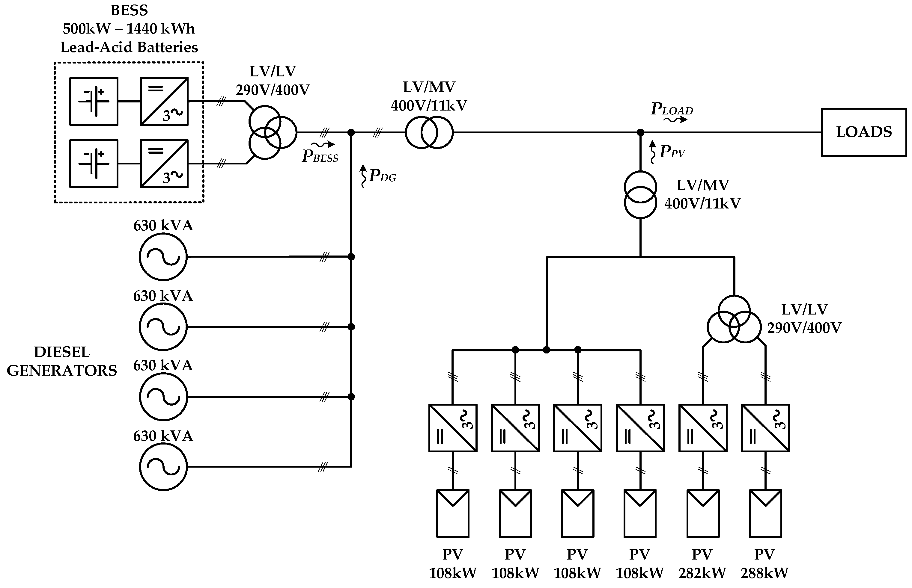
This work takes into account an islanded micro-grid in Garowe City, in the North of Somalia, installed in 2015 [17]. The generation unit can be defined as a Hybrid Power Plant (HPP) because it consists of two different generation systems:

• a conventional generation system, composed of four diesel units of 630 kVA/500kW each;
• a renewable energy system, composed of six PV fields for a total of about 1 MWp.

The electrical system also includes a 2 × 250 kW–2 × 720 kWh BESS, made of two battery banks for a total of 600 lead-acid batteries; each battery is characterized by a rated voltage of 2 V and a rated capacity of 1200 Ah. Each battery bank is connected to the grid through a DC/AC 250 kVA bidirectional inverter. The main function of the BESS is the improvement of the stability of the power plant, with the aim of increasing the exploitation of RES, thereby leading to a substantial fuel economy compared to the solution with only DGs. The plant is designed to supply the city of Garowe through three overhead distribution lines, operating in medium voltage (11 kV, 50 Hz). Since the micro-grid is located in a rural area of Africa, the load is mainly domestic and related to lighting, thus concentrated in the evening hours. Figure 1 shows the diagram of the micro-grid described above.

The HPP is controlled through a system based on Programmable Logic Controllers (PLCs). Normally, it is automatically managed through control logics based on power flow measurements, operational constraints and settings. The actual control logics regulate the power generated by the DGs and the PV and the power generated or absorbed by the BESS. Normally, in order to take the maximum advantage from the solar energy, PV plant is managed with the Maximum Power Point Tracking (MPPT) algorithm, using the Perturb and Observe (P&O) method. The P&O method adopted is based on a trial and error procedure in finding and tracking the MPP, even during variations of the irradiance and temperature [18]. The P&O MPPT algorithm works well when the irradiance changes slowly and so, it should be the most appropriate method for the tropical, hot and dry weather of Somalia.

In case the power production, both from PV and DGs, exceeds the load demand and BESS is not available to store energy, PV is regulated by reducing the power with the algorithm of Regulated Power Point Tracking (RPPT). Anyway, DGs are regulated in order to guarantee an adequate spinning reserve.

The control logics are currently organized in a hierarchical order, based on the relevance and time of implementation of the actions. Functions with the maximum priority are related to safety operations, like prevention of anti-motoring of DG or rapid curtailment of generation. Then functions with medium priority manage the power flows to determine the stability of the micro-grid. In the end, functions with the lowest priority deal with the preservation of the main components, for instance by handling the number of starts and stops of DGs to exploit them in the same way.

2.2. Current Micro-Grid Control Logics

The current control logics do not lead to the best mix of power that allow one to take the maximum advantage from the RES. For that reason, this work aims to verify if an additional level of control, e.g., a tertiary regulation based on forecasting and an optimization method, will be useful to increase the amount of energy produced by RES. In this perspective, the optimized power flows would be inserted into the control logics, as medium-time control [19].

The management of DGs is based on load demand, according to the operational constraints, as minimum and maximum power, and spinning reserve.

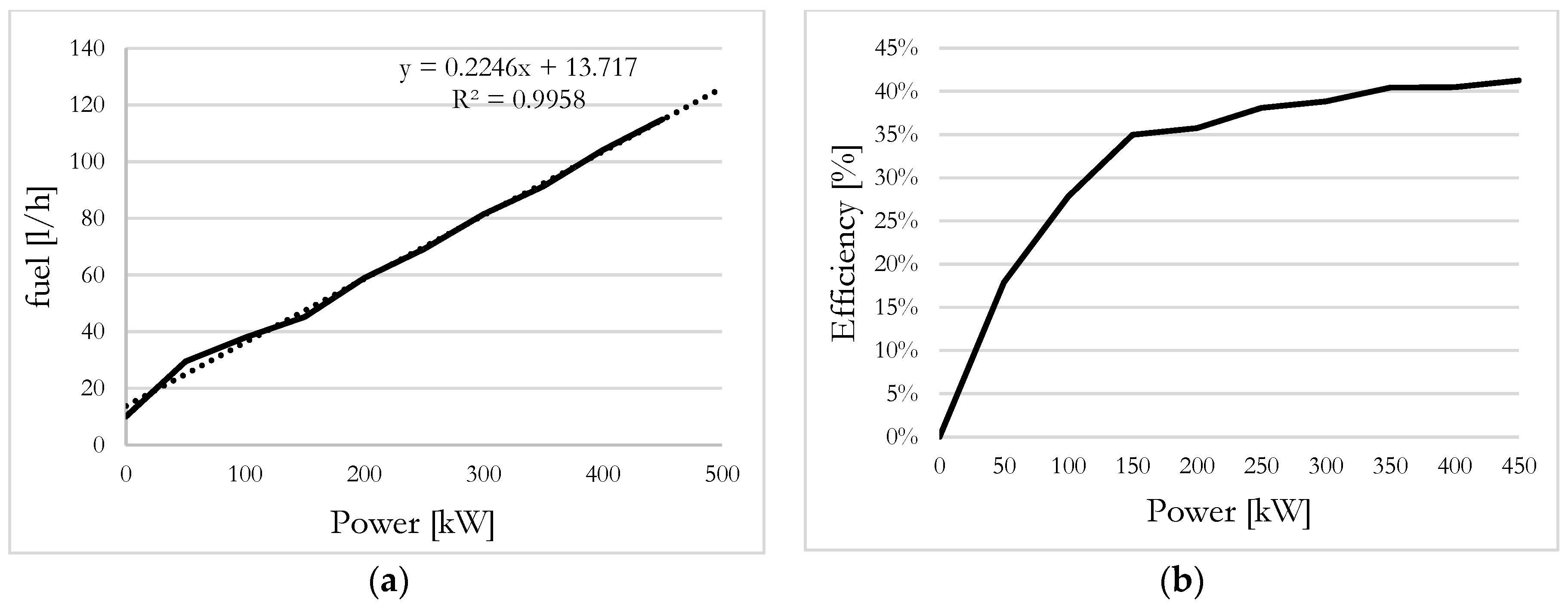
The fuel use has been computed from real measurements of this case study micro-grid. The pairs of experimental values of fuel consumption as a function of the output power have been fitted with a linear regression (Figure 2a), thus the linear dependence between DG power and diesel consumption is:

$$fue{l}_{t,i}=A\cdot u_{t,i}+B\cdot P_{DG,t,i}\forall t\in T,\forall i\in I$$

(1)

where A = 13.717 (L/h) and B = 0.2246 (L/kWh) are the coefficients deduced from the linear regression, u_t,i is a binary variable that represents the on or off status of DG_i at time interval t and P_DGt,i is the DG_i power at time interval t.

By having collected the fuel consumption rates for different power levels of diesel generators, having assumed 40.9 MJ/kg of diesel heating value and 835 kg/m³ for diesel density, it has been possible to calculate the input power for DGs and the corresponding efficiency (Figure 2b).

The spinning reserve of a generator corresponds to its regulating capacity, such as the free power; it can be estimated as the difference between the maximum power of the generator and the power at which it is running at that moment. In order to guarantee a complete load coverage, the available spinning reserve of all the generators at any time must be greater than the required spinning reserve of the system. In this case study, the micro-grid spinning reserve, P_{SR_TOT}, is calculated as maximum the between a fixed term SR_load and a variable one, P_PV, that corresponds to the photovoltaic power produced; SR_load is estimated as the maximum load variation observed in the historical data available, corresponding to 250 kW.

$$P_{sr\_tot}=\max \left\{S{R}_{load},P_{pv,t}\right\}$$

(2)

In this way, during night time the HPP is regulated in order to cover the possible maximum load variation while, during day time the HPP is able to support the maximum generation oscillation.

This solution has been carried out since the demand is completely covered by residential loads, so that load variations compared to the HPP rated power are very limited, whereas a sudden lack of solar power can be responsible for a large oscillation. Moreover, a reduction in irradiation will affect all of the PV inverters, causing a sharp loss of produced power. Thus, it can be considered the worst condition, if compared to a breakdown of a single PV inverter. For this reason, while PV is generating power, the HPP spinning reserve corresponds to the whole PV generation at that moment.

The HPP spinning reserve is supplied by all the generators with regulating capacity, namely by DGs and BESS. BESS participation toward the spinning reserve is fixed at 200 kW. DGs power dedicated to the spinning reserve is calculated as the difference between the total requested spinning and the part of spinning reserve given by the batteries.

The BESS is normally regulated with droop control [20] within a distributed control system [21], in order to support the DGs in performing primary and secondary regulation, thus guaranteeing the power balance of the micro-grid. When BESS primary regulation is not working, the batteries perform a daily cycle of charge and discharge, from 35% to 100% of usable state of charge (SOC). Since the maximum Depth of Discharge (DOD) is 40% (corresponding to 60% of absolute SOC), the limit thresholds expressed in terms of absolute SOC are 74% and 100%. These thresholds have been selected according to the battery supplier’s recommendations and considering the best tradeoff for battery ageing, energy availability and power balance.

2.3. The Sample Day

The sample day that has been chosen among the first six months of operation of the power plant is 17 November 2015, as a representative day for the typical behavior of the case study micro-grid. In order to evaluate the solar production, a comparison between PV measured power and the maximum theoretical power that this PV plant could have generated, at the same ambient conditions of temperature and irradiance, has been carried out.

The maximum harvestable power from PV generators is the ideal power that derives from the MPPT fulfillment and it has been calculated according to [22]:

$$P_{MPPT}=P_{MPP@STC}(1+\gamma \cdot \Delta T)\cdot \frac{G}{G_{STC}}$$

(3)

where, P_MPP@STC is the maximum power at the Standard Test Conditions (STC) of the whole PV system, corresponding to 1 MW; γ is the temperature coefficient corresponding to −0.42%/°C; ΔT is the difference between measured ambient temperature and 25 °C; G is the measured local irradiance (W/m²); G_STC is the irradiance at STC, namely 1000 W/m².

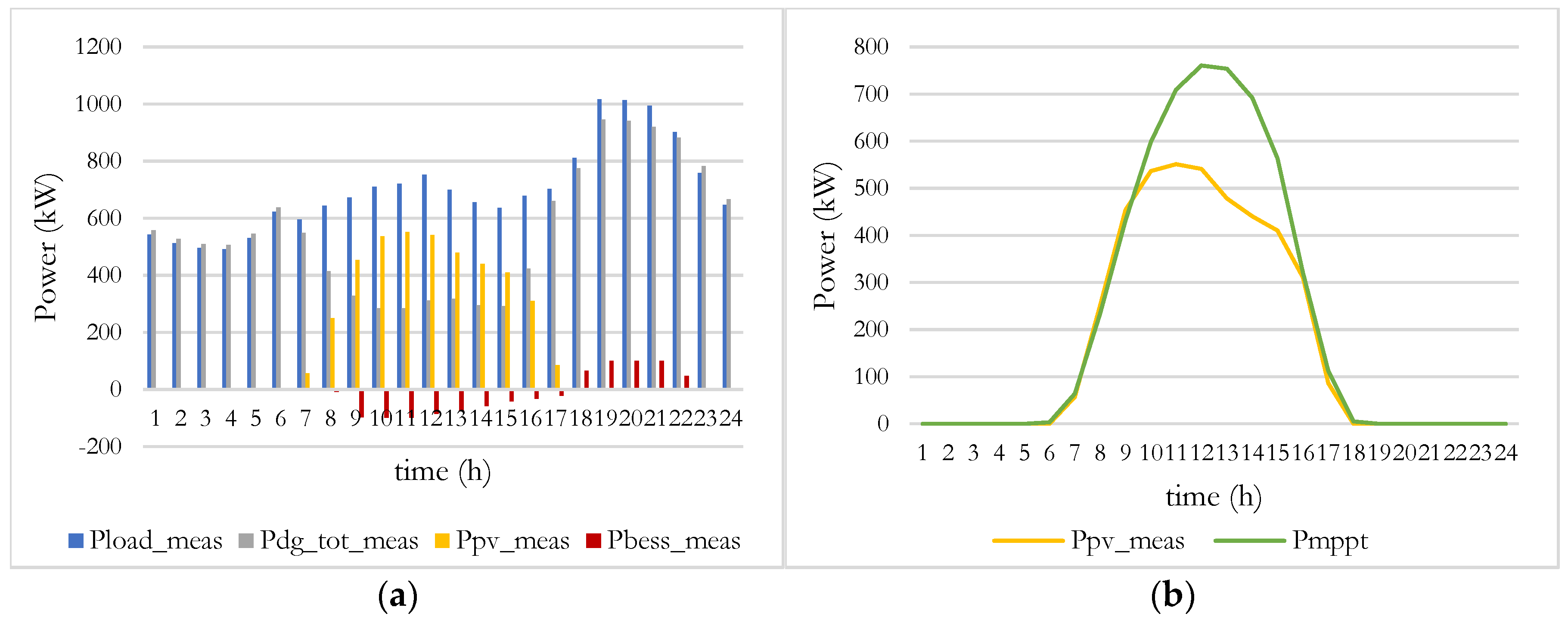
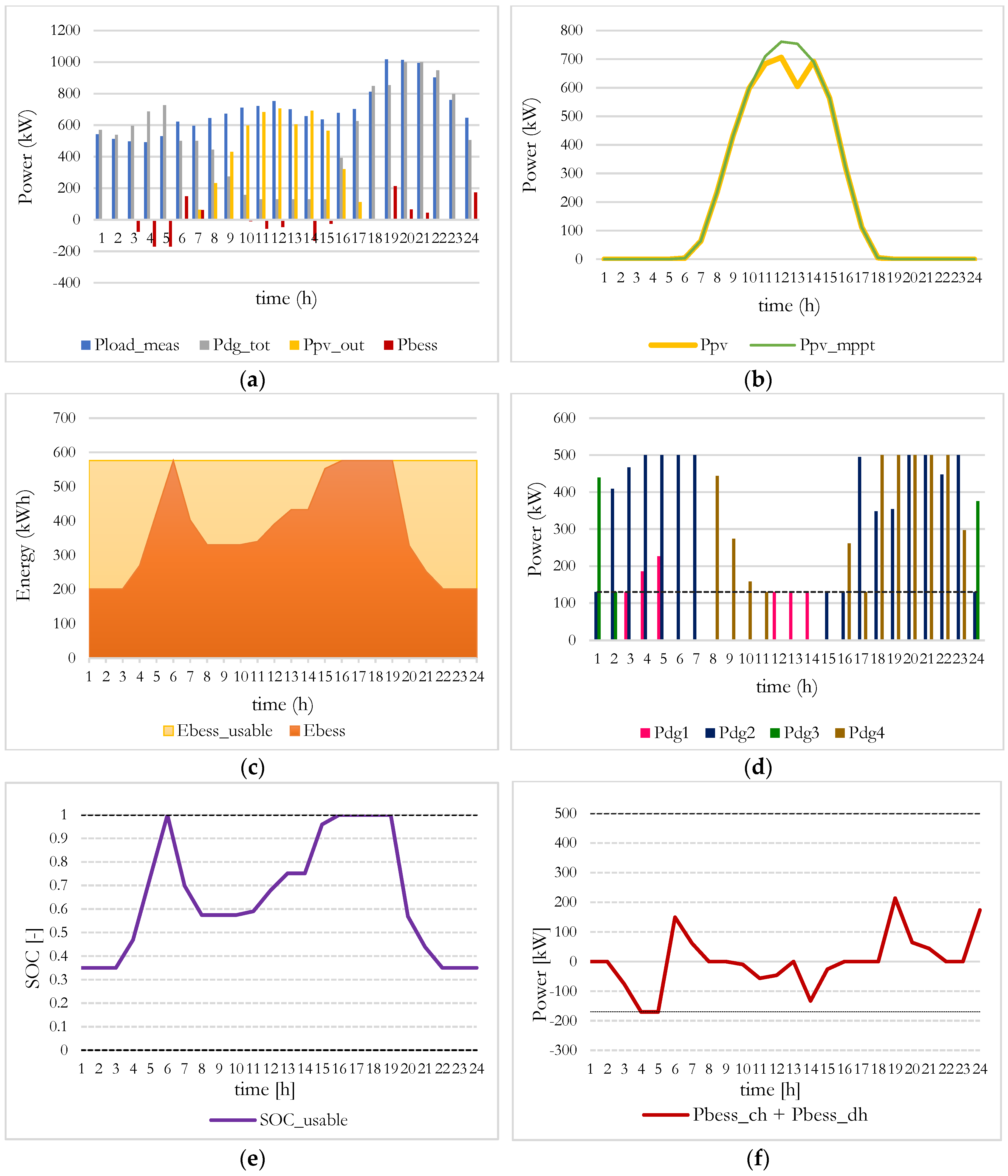
Figure 3a shows the main power flows into the micro-grid case study managed by the actual control logic in terms of power absorbed by the load (Pload_meas), overall power produced by DGs (P_dg_tot_meas), power produced by the PV system (Ppv_meas) and power absorbed (negative values) or generated (positive values) by BESS (Pbess_meas). Figure 3b shows the comparison between the measured PV power (Ppv_meas) and the maximum harvestable power (Pmppt): it is evident that actual power has not reached the maximum possible (for the irradiance conditions of the day analyzed), but it has been curtailed in the central hours of the day.

The PV daily energy that has not been produced is 1131 kWh, corresponding to the 21.5% of the total harvestable PV energy.

3. Linear Programming Model

The first model that has been developed is a simplified optimization problem, based on LP method, implemented with MATLAB software. The code is based on linprog function, applying the Interior Point algorithm. The goal of this optimization model is to evaluate the maximum quantity of RES energy that can be produced into the micro-grid, obtaining a reduction in DGs energy production. The formulation is presented specifying sets (

Table 1. List of sets in the LP model.

Sets	Description	Values	Units
$I$	Set of diesel generators	$\left\{D{G}_1,D{G}_2,...,D{G}_I\right\}$	-
$T$	Set of time intervals	$\left\{t_1,t_2,...,t_T\right\}$	h

), parameters (

Table 2. List of parameters in the LP model.

Parameters	Description	Units
$P_{LOAD,t}$	Load demand forecast at time interval t	kW
$P_{PV,t}$	Photovoltaic production forecast at time interval t	kW

), scalars (

Table 3. List of scalars in the LP model and the set of values used in the case study micro-grid.

Scalar	Description	Value	Unit
${\delta }_{DG,i}^{min};{\delta }_{DG,i}^{max}$	Minimum and maximum operating power for DGi as percentage of $P_{DG,i}^{nom}$	0; 1	p.u.
$SO{C}_{abs}^{min};SO{C}_{abs}^{max}$	Minimum and maximum absolute BESS state of charge	0.6; 1	p.u.
$SO{C}_{1,usable};SO{C}_{T,usable}$	Initial and final value of relative SOC (as percentage of usable energy)	0.35; 0.35	p.u.
$P_{BESS}^{min};P_{BESS}^{max}$	Minimum and maximum BESS power	−170; 500	kW
$P_{DG,i}^{nom}$	Nominal power for DGi	500	kW
$E_{BESS,n}$	Nominal energy capacity of BESS	1440	kWh

) and variables (

Table 4. List of variables in the LP model.

Variables	Description	Units
$E_{BESS}^{min}$	Minimum value of BESS energy	kWh
$E_{BESS}^{max}$	Maximum value of BESS energy	kWh
$E_{BESS}^{max,usable}$	Range of usable BESS energy	kWh
$P_{BESS,t}$	BESS power at time interval t	kW
$P_{DG,t,i}$	DGi power at time interval t	kW
$SO{C}_t$	SOC at time interval t	p.u.
$E_{BESS,t}$	BESS energy at time interval t	kWh
$E_{DG}$	Total DG daily energy produced	kWh

), and describing the related equations. Table 3 summarizes the values of the parameters used in the MIP model.

3.1. Equations of the LP Model

In the followings, the LP optimization model is presented, reporting the set of equations, constraints, parameters and variables that have been used.

• Objective function: since the main purpose of this optimization is to harvest as much of the renewable energy as possible, the objective function of the model has been set as the minimization of the energy production by the DGs, in the time interval considered (T = 24 h).

  $$\min (E_{DG})={\displaystyle \sum _{t=1}^T{\displaystyle \sum _{i=1}^I{P}_{DG,t,i}}}$$

  (4)
• Balance of the power flows: at any time interval, the sum of the power produced by the generators (in the case study, DGs and PV) and the BESS must be equal to the power absorbed by the load (the conventional power flows are shown in Figure 1).

  $${\displaystyle \sum }_{i=1}^I{P}_{DG,t,i}+P_{PV,t}+P_{BESS,t}-P_{LOAD,t}=0\hspace{1em}\forall t \in T$$

  (5)
• Set therange of BESS usable energy, according to the SOC absolute values:

  $$E_{BESS}^{max,usable}=(SO{C}_{abs}^{max}-SO{C}_{abs}^{min})\cdot E_{BESS,n}$$

  (6)
• Set the initial and final value of relative SOC, calculated as percentage of the usable energy, during the period observed:

  $${SO{C}_{usable}|}_{t=1}=SO{C}_{1,usable}$$

  (7)

  $${SO{C}_{usable}|}_{t=T}=SO{C}_{T,usable}$$

  (8)

Instead of using fixed values, generally corresponding to 50% of usable SOC, the unconventional approach of this work is to calculate the final SOC according to the forecasts for the T-period after the considered period (e.g., the day ahead). There are many RES energy production forecasting tools, such as physical models [23], machine learning methods [24] and hybrid models [25]. Hybrid models are represented by any combination of physical models and machine learning methods. The input of the hybrid models are the weather forecast, the geographical coordinates of the site and the date and time to calculate the sun position and the maximum radiation on the PV module; the output is the predicted value of the hourly power produced by the PV plant [26]. Usually, hybrid models are more accurate than pure stochastic methods and physical models [27] and they are suitable for the micro-grid control application. They are trained to recognize the maximum available irradiation and they learn how to reduce the error related to the weather forecasts. Hybrid methods, as well as pure stochastic methods, require a high computation burden, as they have to be trained with a quite long dataset to minimize the forecasting error [28]. In this way, the initial SOC for the day ahead may be more suitable for the tasks of the batteries. In order to set the final SOC, the coefficient R is introduced, as ratio between the energy absorbed by the load, E_LOAD, in the next 24 h and the energy produced by the PV, E_PV, in the same time interval. The following relations have been set up:

$$R=\frac{E_{LOAD}}{E_{PV}}=\frac{{\displaystyle \underset{t=T+1}{\overset{T+24}{\int }}{P}_{LOAD,t}}}{{\displaystyle \underset{t=T+1}{\overset{T+24}{\int }}{P}_{\mathrm{PV},t}}}$$

(9)

$$If\{\begin{array}{lll}R\ge 1& \Rightarrow & SO{C}_{T,usable}={\beta }_1\\ 0.5\le R<1& \Rightarrow & SO{C}_{T,usable}={\beta }_2\\ R<0.5& \Rightarrow & SO{C}_{T,usable}={\beta }_3\end{array}$$

(10)

It has been defined that, if R ≥ 1, meaning a predominance of load consumption over PV production, the initial SOC shall be high in order to provide a large reservoir of storage energy to support RES power. In case 0.5 ≤ R < 1, SOC shall have a medium value, so that batteries can be adapted to different tasks. If R < 0.5, meaning a larger PV generation rather than load consumption, SOC is suggested to be a low value, so that the batteries can store the excess of energy produced by the PV.

According to several attempts, it has been pointed out that the best values for coefficients β₁, β₂, β₃, for the case study micro-grid are:

$$\{\begin{array}{l}{\beta }_1=0.8\\ {\beta }_2=0.5\\ {\beta }_3=0.3\end{array}$$

(11)

• Set the initial and final value of BESS energy, during the period observed, depending on SOC values:

  $${E_{BESS}|}_{t=1}={SOC|}_{t=1}\cdot E_{BESS}^{usable}$$

  (12)

  $${E_{BESS}|}_{t=T}={SOC|}_{t=T}\cdot E_{BESS}^{usable}$$

  (13)
• BESS energy calculation: it is obtained from the energy stored at previous time interval and considering BESS average power in the current interval. BESS efficiency cannot be introduced since it presents a not symmetric behavior in the stored energy calculation during charge and discharge (see later Equation (25)), while LP allows one to implement a single equation. Power is subtracted from energy at time interval t, in order to increase the amount of available energy, in case of power absorbed (taken with negative sign), or to decrease the available energy in case of power delivered to the grid (taken with positive sign).

  $$E_{BESS,t+1}=E_{BESS,t}-P_{BESS,t}\cdot \Delta t \forall t \in T$$

  (14)
• Minimum and maximum DG power: DG power must be limited according to the minimum and maximum operating power of the generators. These values must be set according to the ratings provided by the manufacturer.

  $${\delta }_{DG,i}^{min}\cdot P_{DG,i}^{nom}\le P_{DG,t,i}\le {\delta }_{DG,i}^{max}\cdot P_{DG,i}^{nom}\forall i\in I,\forall t\in T$$

  (15)
• Minimum and maximum BESS power: BESS power must be limited according to the maximum positive and negative power of the inverter and to the maximum C_rate of the batteries.

  $$P_{BESS}^{min}\le P_{BESS,t}\le P_{BESS}^{max}\forall t\in T$$

  (16)
• Minimum and maximum BESS energy: BESS energy range of variation must be limited according to the indications of the battery manufacturer, depending on the technology of the cell. BESS energy must vary within the maximum usable range.

  $$0\le E_{BESS,t}\le E_{BESS}^{max,usable}\forall t\in T$$

  (17)

3.2. Application of LP Model to the Case Study

The LP model has been applied to the sample day, with the values of parameters listed in Table 3. The model has been realized using the measured load power of the real micro-grid in the considered time interval. For PV forecast, as described in the following paragraph, the MPPT power is considered instead of PV forecast or PV measures. The reason for not using forecasted data is to compare the real management of the HPP to the results of the optimization with the same conditions. In this way, the single difference between them is the power and energy profile of the regulating generators (DGs and BESS). Moreover, it is possible to remove the uncertainty introduced by the weather forecast, so that results will not be affected by this further level of uncertainty. The model has been designed for hourly samples.

At first, the use of PV power in the optimization model has been analyzed: as it can be noticed by Figure 4, the output PV power of the optimization model exactly corresponds to the MPPT power; thus, the model allows PV plant to produce the maximum available power.

Moreover, the total energy produced by DGs as output of the optimization model is 11,559 kWh, instead of 13,361 kWh of the actual power plant; thus, the result of the model brings to a 13.5% reduction of the electric energy produced by using fossil fuel (

Table 5. Comparison between case study and LP model’s results.

Data	Measure of Case Study	LP
DG daily energy produced (kWh)	13,361	11,559
DG daily energy saved (%)	-	13.5
PV energy not produced for RPPT (kWh)	1131 (21.5% of total energy)	0
DG daily fuel cost (€)	2699	2812.38
DG daily cost saved (%)	-	−113.38 (−4%)

).

From these statements, it can be observed that, applying the optimization model using LP, with respect to the real-time control logics of the micro-grid the following benefits can be achieved:

• use of RPPT algorithm as less as possible and better exploitation of PV power;
• less electric energy produced by using fossil fuel, as a consequence of the previous benefits;
• possibility to set up a schedule for the day ahead, for BESS and DG production (by means of forecasting data as inputs of the optimization model).

The LP model, however, does not allow to represent the switching on and switching off of the DGs, since LP requires the use of continuous variables, denying discrete variables; in this way, it imposes them to be operated at any time and at the same power rate. When a small amount of power is required to be produced by the DGs, their operating point is lower than the minimum recommended (25% of nominal active power). The main drawback is that, in the range between zero and the minimum operating power, the efficiency of DGs is dramatically low, increasing the fuel consumption. It can be noticed from Figure 4 that DG power stays under the minimum operating limit for about 45% of the day. For the same reason, the minimization of the energy produced by the DG implemented in LP as objective function may not correspond to a minimization of the fuel consumption and relative costs, in particular when more than one generator is considered. It can be noticed from Table 5 that the overall cost for the LP model is 4% higher than in the real case, even with an increase of the solar power production of 21.5%. Thus, a further development of the work has been dedicated to develop a more detailed model with a new objective function focused on the minimization of the operating costs. In this case, MIP will be used in order to overcome the limitations of the LP, since the model requires the use of discrete variables (e.g., DG start/stop).

4. Mixed Integer Programming Model

The second model that has been developed is a MIP optimization model. It has been selected the MIP as optimization method since, unlike LP, it allows modelling discrete (binary) variables. The binary variables have been used in the model to represent the start up and shut down state of DGs and to distinguish between charge and discharge phase of batteries [29].

As for the LP method, the formulation is presented specifying sets (

Table 6. List of sets in the MIP model.

Sets	Description	Values	Units
$I$	Set of diesel generators	$\left\{D{G}_1,D{G}_2,...,D{G}_I\right\}$	-
$T$	Set of time intervals	$\left\{t_1,t_2,...,t_T\right\}$	H

), parameters (

Table 7. List of parameters in the MIP model.

Parameters	Description	Units
$P_{LOAD,t}$	Load demand forecast at time interval t	kW
$P_{PV,t}$	Photovoltaic production forecast at time interval t	kW

), scalars (

Table 8. List of scalar in the MIP model and set of values used in the case study micro-grid.

Scalar	Description	Value	Unit
${\eta }_{BESS}^{ch}$	BESS charging efficiency	0.90	p.u.
${\eta }_{BESS}^{dh}$	BESS discharging efficiency	0.86	p.u.
$SO{C}_{usable}^{min};SO{C}_{usable}^{max}$	Minimum and maximum usable BESS state of charge	0, 1	p.u.
$SO{C}_{1,usable};SO{C}_{T,usable}$	Initial and final value of SOC	0.35; 0.35	p.u.
$P_{BESS}^{ch,min};P_{BESS}^{ch,max}$	Minimum and maximum BESS charging power	−170; 0	kW
$P_{BESS}^{dh,min};P_{BESS}^{dh,max}$	Minimum and maximum BESS discharging power	0; 500	kW
$\alpha$	Fraction of PV power to be covered with spinning reserve	1	p.u.
$S{R}_{LOAD}$	Amount of load power to be covered with spinning reserve	250	kW
$\lambda$	Auxiliary services power, as percentage of PLOAD,t	0.05	p.u.
$P_{DG,i}^{nom}$	Nominal power for DGi	500	kW
${\delta }_{DG,i}^{min};{\delta }_{DG,i}^{max}$	Minimun and maximum operating power for DGi as percentage of $P_{DG,i}^{nom}$	0.26; 1	p.u.
$C_{DG,i}^{su};C_{DG,i}^{sd}$	Start up and shut down cost for DGi	0, 0	€
$C_f$	Cost of fuel	0,75	€/l
$C_{curt,t}$	Cost of curtailed PV power	0	€/kWh
$N_{DG}^{max,start}$	Maximum number of DG starts in a day	2	-
$N_{DG}^{min,off}$	Minimum duration of time off of DGi	0	S
$E_{BESS,usable}$	Nominal energy capacity of battery storage system	576	kWh

) and variables (

Table 9. List of variables in the MIP model.

Variables	Description	Units
$P_{BESS,t}^{ch}$	BESS charging power at time interval t	kW
$P_{BESS,t}^{dh}$	BESS discharging power at time interval t	kW
$P_{DG,t,i}$	DGi power at time interval t	kW
$P_{PVcurt,t}$	PV power curtailed at time interval t	kW
$SO{C}_{t,usable}$	Usable SOC at time interval t	p.u.
$P_{AUX,t}$	Auxiliary services power at time interval t	kW
$u_{t,i}$	On/Off status of DGi at time interval t, $u_{t,i}\in \left\{0,1\right\}$	-
$x_{t,i}$	Charging status of BESS at time interval t, $x_{t,i}\in \left\{0,1\right\}$	-
$s{u}_{t,i}$	Start up flag for DGi at time interval t, $s{u}_{t,i}\in \left\{0,1\right\}$	-
$s{d}_{t,i}$	Shut down flag for DGi at time interval t, $s{d}_{t,i}\in \left\{0,1\right\}$	-
$Cost$	Total operating cost	€
$S{R}_{tot,up,t}$	Total spinning reserve up at time interval t	kW
$S{R}_{tot,dwn,t}$	Total spinning reserve down at time interval t	kW
$S{R}_{DGup,t,i}$	Spinning reserve up of DGi at time interval t	kW
$S{R}_{DGdwn,t,i}$	Spinning reserve down of DGi at time interval t	kW
$S{R}_{BESSup,t}$	BESS spinning reserve up at time interval t	kW
$S{R}_{BESSdwn,t}$	BESS spinning reserve down at time interval t	kW

), and describing the equations. Table 8 summarizes the values of the parameters used into the MIP model. The MIP model has been developed with General Algebraic Modeling System (GAMS) software, using the CPLEX solver [30]. In the following, the formulation of the optimization is presented.

4.1. Equations of the MIP Model

The objective function corresponds to the minimization of the total operating costs over the whole period T. The new objective function is the main difference with respect to LP programming model, where minimization of the energy produced by DGs was defined as the main goal. The total operating costs are determined by the fuel cost C_f, which is a function of the power of each DG at each time interval, cost associated with the start-up and shut-down of DG, and costs due to curtailment of PV power [31].

$$\min (Cost)=\min \left({\displaystyle \sum _{t=1}^T\left({\displaystyle \sum _{i=1}^I\left(C_f\left(P_{DG,t,i}\right)+s{u}_{t,i}\cdot C_{DG,i}^{su}+s{d}_{t,i}\cdot C_{DG,i}^{sd}\right)}\right)}+{\displaystyle \sum _{t=1}^T\left(P_{PVcurt,t}\cdot C_{curt,t}\right)}\right)$$

(18)

• Power balance: at any time interval, the sum of the power produced by generators (DG, PV and BESS) must meet the power absorbed by the load, taking into account also the power absorbed by the auxiliary services of the power plant. The equation comprehends the term P_PV,t, that is the forecasted PV production to which the term P_PVcurt,t is subtracted, in order to obtain the effective amount of PV power produced [32].

  $${\displaystyle \sum }_{i=1}^I{P}_{DG,t,i}+P_{PV,t}+P_{BESS,t}^{dh}+P_{BESS,t}^{ch}-P_{PVcurt,t}-P_{AUX,t}-P_{LOAD,t}=0\forall t\in T$$

  (19)
• Calculation of the power absorbed by the auxiliary services of the power plant, assuming it is proportional to load power.

  $$P_{AUX,t}=\lambda \cdot P_{LOAD,t} \forall t \in T$$

  (20)
• Calculation of PV curtailed power and PV power actually produced.

  $${\displaystyle \sum }_{i=1}^I{P}_{DG,t,i}+P_{PV,t}+P_{BESS,t}^{dh}+P_{BESS,t}^{ch}-P_{AU{X}_t}-P_{LOAD,t}=P_{PVcurt,t}\forall t \in T$$

  (21)

  $$P_{PVout,t}=P_{PV,t}-P_{PVcurt,t}\forall t \in T$$

  (22)
• Setting the initial and final value of SOC, with respect to the total time T:

  $${SO{C}_{usable}|}_{t=1}=SO{C}_{1,usable}$$

  (23)

  $${SO{C}_{usable}|}_{t=T}=SO{C}_{T,usable}$$

  (24)

Similar considerations about initial and final values for SOC, carried out for the LP model, can be applied even for MIP problem.

• SOC calculation: since the model implements usable SOC, it has to be calculated through power variation over each time interval, with respect to the usable energy. Charging and discharging power are separately considered [33].

  $$SO{C}_{t+1,usable}=SO{C}_{t,usable}-\frac{\Delta t({\eta }_{BESS}^{ch}{P}_{BESS,t}^{ch}+\frac{P_{BESS,t}^{dh}}{{\eta }_{BESS}^{dh}})}{E_{BESS,usable}}\forall t\in T$$

  (25)
• Total up and down spinning reserve calculation: as for the control of the micro-grid case study, spinning reserve is calculated as the maximum between a term depending on PV power at each time interval and a fixed term depending on the maximum load oscillation.

  $$S{R}_{tot,up,t}=S{R}_{tot,dwn,t}=\max \left\{\alpha \cdot P_{pv,t},S{R}_{LOAD}\right\}\forall t\in T$$

  (26)
• DG and BESS up/down spinning reserve calculation: the total amount of spinning reserve provided by the all the regulating generators (DGs and BESS) must be equal or greater than the spinning reserve required [34,35].

  $${\displaystyle \sum _{i=1}^{I}S{R}_{DGup,t,i}+S{R}_{BESSup,t}\ge S{R}_{tot,up,t}\forall t\in T}$$

  (27)

  $${\displaystyle \sum _{i=1}^{I}S{R}_{DGdwn,t,i}+S{R}_{BESSdwn,t}\ge S{R}_{tot,dwn,t}\forall t\in T}$$

  (28)
• Start-up and shut-down status of DG: they are calculated comparing the DG status at present time interval with the one at previous time interval.

  $$s{u}_{t,i}-s{d}_{t,i}=u_{t,i}-u_{(t-1),i}\hspace{1em}\hspace{1em}\forall i \in I,\hspace{1em}\hspace{1em}\forall t \in T$$

  (29)
• Maximum number of DG start and stop events: this constraint is set in order to prevent an excessive stress on the generators.

  $${\displaystyle \sum _{t=1}^{T}s{u}_{t,i}}\le N_{DG}^{max,start}\forall i\in I$$

  (30)
• Minimum and maximum DG power, considering on/off flag and spinning reserve margins. DG power must be limited according to the minimum and maximum operating power of the generators. These values must be set accordingly to the statements of the manufacturer; longer functioning at lower power is not recommended, because it reduces efficiency and could affect useful lifetime [36,37].

  $$u_{t,i}\cdot {\delta }_{DG,i}^{min}\cdot P_{DG,i}^{nom}+S{R}_{DGdwn,t,i}\le P_{DG,t,i}\le u_{t,i}\cdot {\delta }_{DG,i}^{max}\cdot P_{DG,i}^{nom}-S{R}_{DGup,t,i}\forall i\in I,\forall t\in T$$

  (31)
• Minimum and maximum BESS power, considering charge or discharge flag. BESS power must be limited according to the rated power of the inverter and to the maximum C_rate of the batteries.

  $$x\cdot P_{BESS}^{ch,min}\le P_{BESS,t}^{ch}\le x\cdot P_{BESS}^{ch,max} \forall t \in T$$

  (32)

  $$(1-x)\cdot P_{BESS}^{dh,min}\le P_{BESS,t}^{dh}\le (1-x)\cdot P_{BESS}^{dh,max} \forall t \in T$$

  (33)
• Minimum and maximum SOC of the battery bank. Operating range of SOC corresponds to the usable SOC.

  $$SO{C}_{usable}^{min}\le SO{C}_{t,usable}\le SO{C}_{usable}^{max} \forall t \in T$$

  (34)
• Minimum and maximum SOC, taking into account spinning reserve margins.

  $$SO{C}_{usable}^{min}+\frac{S{R}_{BESSup,t}}{E_{BESS,usable}}\le SO{C}_{t,usable}\le SO{C}_{usable}^{max}-\frac{S{R}_{BESSdwn,t}}{E_{BESS,usable}} \forall t \in T$$

  (35)
• Minimum and maximum BESS power, taking into account spinning reserve margins.

  $$P_{BESS,t}^{dh}+P_{BESS,t}^{ch}+S{R}_{BESSup,t}\le P_{BESS}^{dh,max}\forall t\in T$$

  (36)

  $$P_{BESS,t}^{dh}+P_{BESS,t}^{ch}-S{R}_{BESSdwn,t}\ge P_{BESS}^{ch,min}\forall t\in T$$

  (37)

4.2. Application of the MIP Model to the Case Study

The inputs of the model are, as for LP problem, the measured load power absorbed during the 24 h analyzed and the PV power calculated at MPP conditions.

Considering the use of DGs, it can be pointed out from Figure 5 that each generator operates within the range of 26% and 100% of rated active power (respectively, 130 kW and 500 kW). If needed, one or more generators can be turned off, but they never work at power levels lower than the minimum operating threshold. This is an important improvement with respect to LP model, where DGs power varies continuously from zero to the maximum. Such management is extremely relevant for the minimization of the fuel consumption, because the generators do not equally share the total required power and they are working in a more efficient condition [38], as it can be noticed from Figure 2b. The total daily cost associated to the fuel consumption, which is part of the objective function in the MIP model, comes from Equation (1):

$${\displaystyle \sum _{t=1}^T{\displaystyle \sum _{i=1}^I{C}_f(P_{DG,t,i})}}={\displaystyle \sum _{t=1}^T{\displaystyle \sum _{i=1}^I{C}_f\cdot (u_{t,i}\cdot A+B\cdot P_{DG,t,i})}}$$

(38)

where A and B are the coefficients of the linear dependence between DG power and diesel consumption and u_t,i is the binary variable that represent the on or off status of DG_i at time interval t, already defined along with Equation (1).

Unlike the actual control logics that assigns to BESS spinning reserve a fixed value of 200 kW, the MIP model implements a free allocation of BESS spinning reserve. The choice to let free the BESS amount of spinning reserve allows assigning a greater amount of spinning reserve to the BESS with respect to the actual control logics, especially during the central hours of day (Figure 6a).

Therefore, the amount of spinning reserve allocated to the DGs in the middle of day decreases (Figure 6b). In this way, the number of DGs working at the same time can be lower than in the actual management, since the total quantity of spinning reserve they have to provide has been reduced, so that just one or two DGs can contribute to it. During the night, the spinning reserve of DGs is greater than in the actual control logic, thus it is not expected to have a strong impact on the number of DGs that are running. In fact, during the night, the load is almost completely covered by DGs (just a little portion by BESS), so that, even if spinning reserve decreases, the number of running DGs cannot be reduced, otherwise load cannot be supplied. As a result, the total daily energy produced by DGs is reduced by 5.8% with respect to the measured value of the case study micro-grid.

Moreover, the optimization model imposes that the DGs are working in a more efficient operating condition, with a 12.3% of fuel savings. Consequently, renewable energy source can be mostly exploited, reducing the curtailed PV energy from 21.5% down to 4.4% of daily energy.

Table 10. Comparison between case study and MIP model’s results.

Data	Measure of Case Study	MIP
DG daily energy produced (kWh)	13,361	12,589
DG daily energy saved (%)	-	5.8
PV energy not produced for RPPT (kWh)	1131 (21.5% of total energy)	230 (4.4% of total energy)
DG daily fuel cost (€)	2699	2366
DG daily cost saved (%)	-	12.3%

summarizes the main comparison between the actual behavior of the HPP (measured values) and the results of the MIP optimization model, in terms of DG energy and fuel consumption saved, and reduction of PV energy curtailed. Comparing the MIP model’s results to the actual management of the micro-grid, it can be pointed out that there is an improvement both in terms of RES use and DGs fuel consumption.

In terms of solar energy harvested, results can be worse than LP, in which PV energy is completely exploited and DG energy saved is more than in MIP model. However, calculating the total operating costs for the LP model, it emerged that total daily cost is 2812€, 4% more than actual costs and 18.8% more than MIP results. This happened because DGs work for almost half of the day with low efficiency (Figure 4), consuming a larger quantity of fuel with high associated costs.

5. Conclusions

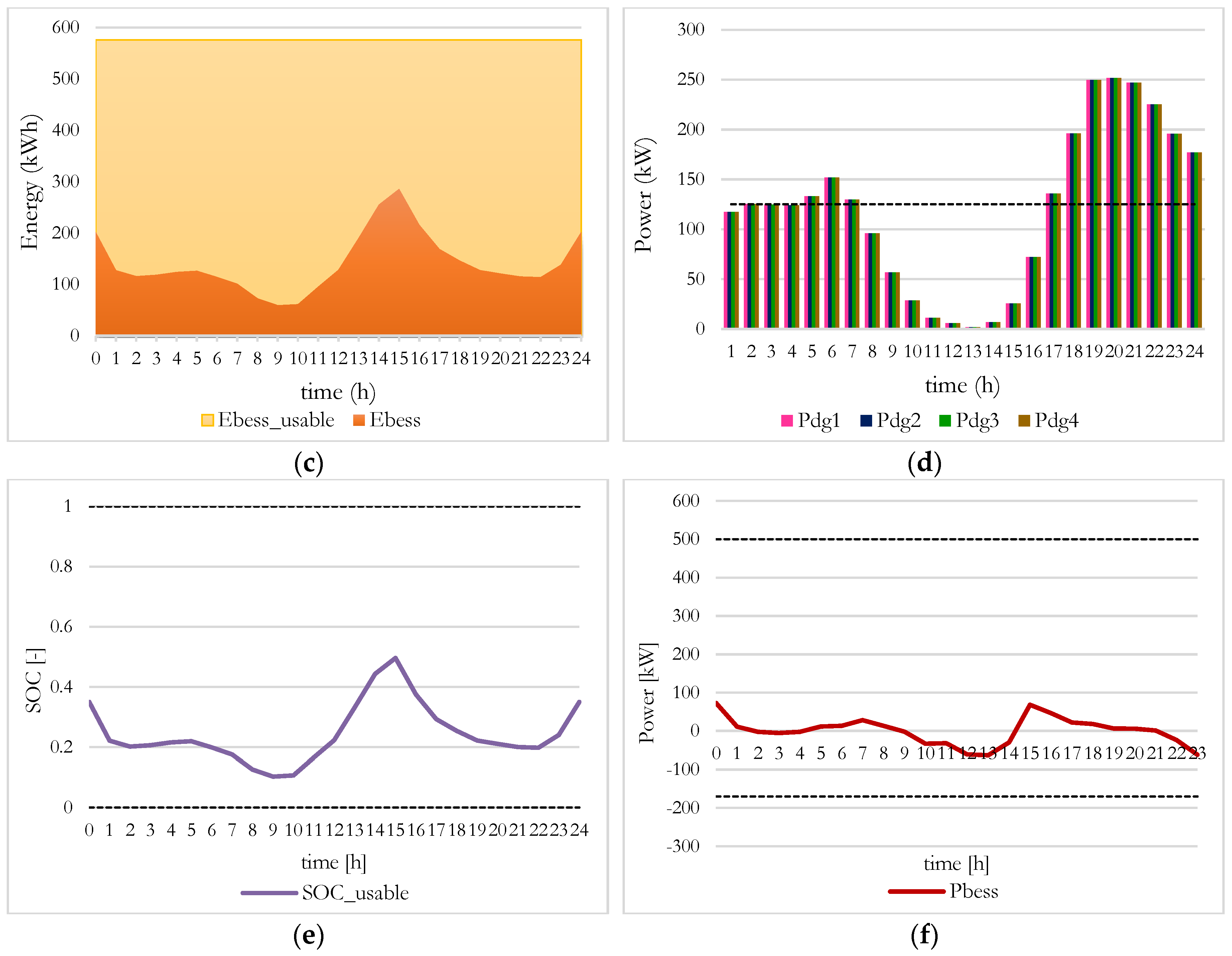
This paper developed and compared two optimization methods intended to define the power flows into an islanded micro-grid including DGs, PV systems and BESS. The LP method has been applied to set up the model to maximize the energy harvesting from renewable energy sources, while the MIP method has allowed to set up the model to minimize the micro-grid operating costs.

An islanded micro-grid, placed in Somalia and running since November 2015, has been identified as case study for this research. It emerged that load profile, with peaks concentrated during evening hours mainly due to lighting and domestic appliances, does not match with the PV generation curve. Since battery storage capacity has not been sized for time-shift function, it cannot store all the excess PV power produced during the day. Moreover, in order to guarantee the required spinning reserve, the actual control logics keep the DGs working close to their minimum power also in case of high PV production. In these conditions, to comply with the power balance, PV power has to be curtailed during the central hours of the day. In the sample day, it appeared that a large part of PV daily energy, equal to 21.5%, cannot be produced due to spinning reserve constraints.

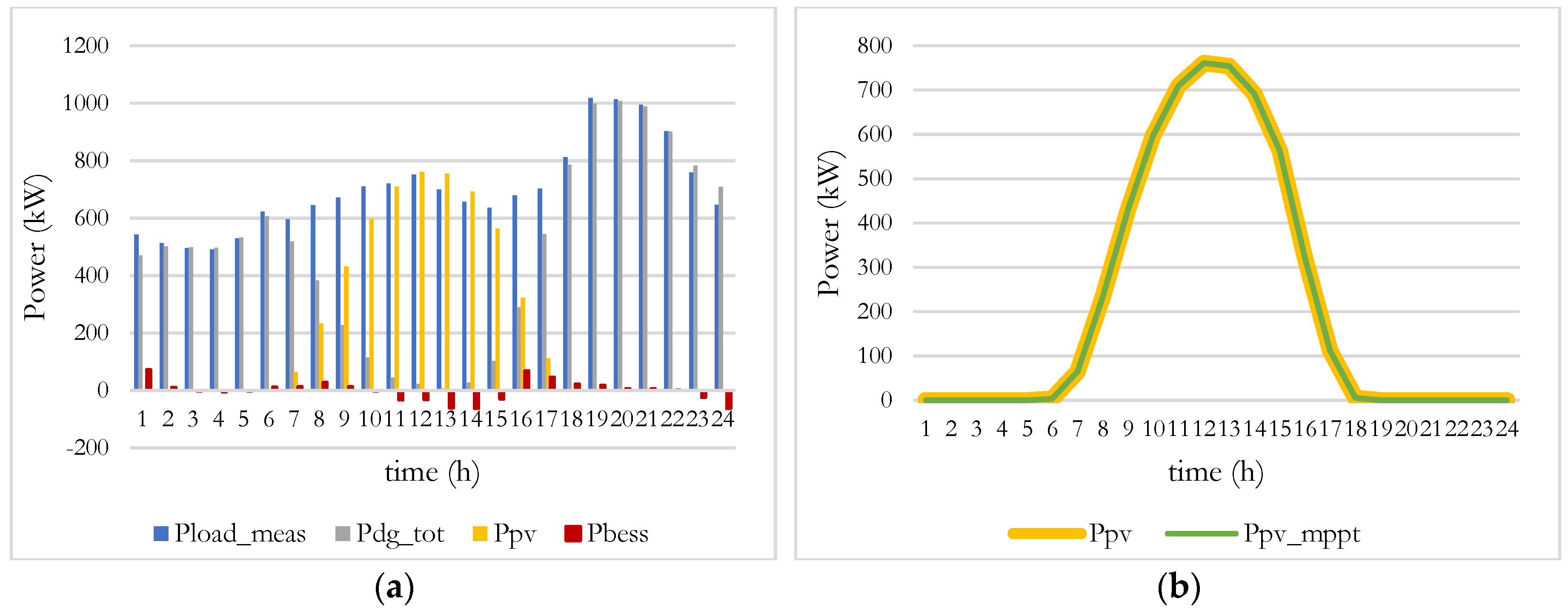
Optimization models allow to improve the actual management by minimizing PV curtailment or operating costs, namely the fuel consumption. The optimization model developed using LP has been formulated in order to minimize the DGs’ energy produced during the day. As a result of the LP model, it can be noticed that the daily electric energy produced by DGs can be reduced by 13.5% and PV energy produced corresponds to the maximum feasible, but overall costs are 4% higher than in the real case study. The LP model imposes the DGs to operate in the range between zero and the minimum operating power, thus with an extremely low efficiency, for several hours per day, resulting in an increase of the fuel consumption. The optimization model developed using MIP has been formulated to overcome this problem, setting the objective function as the minimization of the operating costs. As a result of the MIP model, it can be noticed that the daily fuel cost saving is 12.3%, corresponding to a 5.8% of DG energy saving. The curtailed PV energy reduces from 21.5% to 4.4% of the maximum harvestable solar energy.

MIP model is a more complex and more complete model with respect to the LP model, able to represent real operating management scenarios of the HPP without any limitations. In particular, the modeling of the start and stop of DGs and their independent management is crucial in defining power flows that minimize the use of fossil fuels. Moreover, MIP model allows to point out the limitations of the actual control logics of the case study micro-grid. The improvements in the control logic, related to the optimized approach, can be summarized as:

• let the amount of spinning reserve dedicated to BESS free to be calculated by the optimal solution;
• do not equally share power among DGs, but take care to the best mix of power in order to have the maximum efficiency.

In order to apply further improvements to the management of the micro-grid, two possible solutions can be followed: the first one is the increment of the storage capacity installed, to increase the quantity of RES energy that can be stored in case it exceeds load demand. This could be an effective solution; however, it will not be the least expensive one. The second alternative is the identification of different spinning reserve margins that could lead to an additional reduction in fuel consumption. A possible further development of this work will consider the latter scenario.

Moreover, in order to take into account the benefits of both LP and MIP methods, the design of a new multi-objective model can be implemented, combining the maximization of RES energy harvesting and minimizing the operating costs. However, this approach necessarily requires using specific multi-objective optimization algorithms. A second option can be the definition in the MIP model of a weighted objective function representing a tradeoff of the previous goals.

References

1. Africa Energy Outlook: A Focus on Prospects in Sub-Saharan Africa. Available online: https://www.iea.org/publications/freepublications/publication/WEO2014_AfricaEnergyOutlook.pdf (accessed on 18 December 2016).
2. Doorsamy, W.; Cronje, W.A. Sustainability of decentralized renewable energy systems in Sub-Saharan Africa. In Proceedings of the 4th International Conference on Renewable Energy Research and Applications (ICRERA 2015), Palermo, Italy, 22–25 November 2015.
3. Murenzi, J.P.; Ustun, T.S. The case for microgrids in electrifying Sub-Saharan Africa. In Proceedings of the 2015 6th International Renewable Energy Congress (IREC 2015), Sousse, Tunisia, 24–26 March 2015.
4. Buchana, P.; Ustun, T. The role of microgrids & renewable energy in addressing sub-saharan Africa’s current and future energy needs. In Proceedings of the 2015 6th International Renewable Energy Congress (IREC 2015), Sousse, Tunisia, 24–26 March 2015.
5. Li, Y.W.; Kao, C.N. An accurate power control strategy for power electronics-interfaced distributed generation units operating in a low voltage multibus microgrid. IEEE Trans. Power Electron. 2009, 24, 2977–2988. [Google Scholar]
6. Mercier, P.; Cherkaoui, R.; Oudalov, A. Optimizing a battery energy storage system for frequency control application in an isolated power system. IEEE Trans. Power Syst. 2009, 24, 1469–1477. [Google Scholar] [CrossRef]
7. Lidula, N.W.A.; Rajapakse, A.D. Microgrids research: A review of experimental microgrids and test systems. Renew. Sustain. Energy Rev. 2011, 15, 186–202. [Google Scholar] [CrossRef]
8. Hatziargyriou, N.; Asano, H.; Iravani, R.; Marnay, C. Microgrids. IEEE Power Energy Mag. 2007, 5, 78–94. [Google Scholar] [CrossRef]
9. Karavas, C.S.; Kyriakarakos, G.; Arvanitis, K.G.; Papadakis, G. A multi-agent decentralized energy management system based on distributed intelligence for the design and control of autonomous polygeneration microgrids. Energy Convers. Manag. 2015, 103, 166–179. [Google Scholar] [CrossRef]
10. Kyriakarakos, G.; Dounis, A.I.; Rozakis, S.; Arvanitis, K.G.; Papadakis, G. Polygeneration microgrids: A viable solution in remote areas for supplying power, potable water and hydrogen as transportation fuel. Appl. Energy 2011, 88, 4517–4526. [Google Scholar] [CrossRef]
11. Wierzbowski, M.; Wojciech, L.; Musial, I. MILP model for long-term energy mix planning with consideration of power system reserves. Appl. Energy 2016, 169, 93–111. [Google Scholar] [CrossRef]
12. Riffonneau, Y.; Bacha, S.; Barruel, F.; Ploix, S. Optimal power flow management for grid connected PV systems with batteries. IEEE Trans. Sustain. Energy 2011, 2, 309–320. [Google Scholar] [CrossRef]
13. Tolis, A.I.; Rentizelas, A.A. An impact assessment of electricity and emission allowances pricing in optimised expansion planning of power sector portfolios. Appl. Energy 2011, 88, 3791–3806. [Google Scholar] [CrossRef] [Green Version]
14. Luna, A.C.; Diaz, N.L.; Graells, M.; Vasquez, J.C.; Guerrero, J.M. Mixed-integer-linear-programming-based energy management system for hybrid PV-wind-battery microgrids: Modeling, design, and experimental verification. IEEE Trans. Power Electron. 2017, 32, 2769–2783. [Google Scholar] [CrossRef]
15. Fedjaev, J.; Amamra, S.A.; Francois, B. Linear programming based optimization tool for day ahead energy management of a lithium-ion battery for an industrial microgrid. In Proceedings of the 2016 IEEE International Power Electronics and Motion Control Conference (PEMC), Varna, Bulgaria, 25–28 September 2016.
16. Nugraha, P.Y.; Widyotriatmo, A.; Samsi, A. Optimization of capacity and operational scheduling for microgrid system using two-stage stochastic linear programming. In Proceedings of the International Conference on Instrumentation, Control and Automation (ICA), Institut Teknologi Bandung (ITB), Bandung, Indonesia, 29–31 August 2016.
17. Dolara, A.; Grimaccia, F.; Magistrati, G.; Marchegiani, G. Optimal management algorithm for battery energy storage system included in an islanded micro-grid. In Proceedings of the 16th International Conference on Environment and Electrical Engineering (EEEIC 2016), Florence, Italy, 7–10 June 2016.
18. Karami, N.; Moubayed, N.; Outbib, R. General review and classification of different MPPT Techniques. Renew. Sustain. Energy Rev. 2017, 68, 1–18. [Google Scholar] [CrossRef]
19. Sanseverino, E.R.; Di Silvestre, M.L.; Quang, N.N.; Mineo, L.; Guerrero, J.M.; Luna, A.C.; Vasquez, J.C.; Graells, M. Energy management systems and tertiary regulation in hierarchical control architectures for islanded microgrids. In Proceedings of the 15th IEEE International Conference on Environment and Electrical Engineering (EEEIC 2015), Rome, Italy, 10–13 June 2015.
20. Vasquez, J.C.; Guerrero, J.M.; Savaghebi, M.; Eloy-Garcia, J.; Teodorescu, R. Modelling, analysis and design of stationary reference frame droop controlled parallel three-phase voltage source inverters. In Proceedings of the 8th International Conference on Power Electronics—ECCE Asia: “Green World with Power Electronics” (ICPE 2011-ECCE Asia), Jeju, Korea, 30 May–3 June 2011.
21. Guerrero, J.M.; Matas, J.; De Vicuña, L.G.; Castilla, M.; Miret, J. Wireless-control strategy for parallel operation of distributed-generation inverters. IEEE Trans. Ind. Electron. 2006, 53, 1461–1470. [Google Scholar] [CrossRef]
22. Photovoltaic System Performance Monitoring Guidelines for Measurement, Data Exchange and Analysis; CEI EN 61724; International Electrotechnical Commission: Geneva, Switzerland, 1999.
23. Dolara, A.; Leva, S.; Manzolini, G. Comparison of different physical models for PV power output prediction. Sol. Energy 2015, 119, 83–99. [Google Scholar] [CrossRef] [Green Version]
24. Leva, S.; Dolara, A.; Grimaccia, F.; Musetta, M.; Ogliari, E. Analysis and validation of 24 hours ahead neural network forecasting of photovoltaic output power. Math. Comput. Simul. 2017, 131, 88–100. [Google Scholar] [CrossRef] [Green Version]
25. Ogliari, E.; Grimaccia, F.; Leva, S.; Mussetta, M. Hybrid predictive models for accurate forecasting in PV systems. Energies 2013, 6, 1918–1929. [Google Scholar] [CrossRef] [Green Version]
26. Gandelli, A.; Grimaccia, F.; Leva, S.; Mussetta, M.; Ogliari, E. Hybrid model analysis and validation for PV energy production forecasting. In Proceedings of the 2014 International Joint Conference on Neural Networks (IJCNN 2014), Beijing, China, 6–11 July 2014.
27. Dolara, A.; Grimaccia, F.; Leva, S.; Mussetta, M.; Ogliari, E. A physical hybrid artificial neural network for short term forecasting of PV plant power output. Energies 2015, 8, 1138–1153. [Google Scholar] [CrossRef] [Green Version]
28. Dolara, A.; Leva, S.; Mussetta, M.; Ogliari, E. PV hourly day-ahead power forecasting in a micro grid context. In Proceedings of the 16th International Conference on Environment and Electrical Engineering (EEEIC 2016), Florence, Italy, 7–10 June 2016.
29. Hu, C.; Luo, S.; Li, Z.; Wang, X.; Sun, L. Energy coordinative optimization of wind-storage-load microgrids based on short-term prediction. Energies 2015, 8, 1505–1528. [Google Scholar] [CrossRef]
30. Borghetti, A.; D’Ambrosio, C.; Lodi, A.; Martello, S. An MILP approach for short-term hydro scheduling and unit commitment with head-dependent reservoir. IEEE Trans. Power Syst. 2008, 23, 1115–1124. [Google Scholar] [CrossRef]
31. Bischi, A.; Taccari, L.; Martelli, E.; Amaldi, E.; Manzolini, G.; Silva, P.; Campanari, S.; Macchi, E. A detailed MILP optimization model for combined cooling, heat and power system operation planning. Energy 2014, 74, 12–26. [Google Scholar] [CrossRef]
32. Lazaroiu, G.C.; Dumbrava, V.; Balaban, G.; Longo, M.; Zaninelli, D. Stochastic optimization of microgrids with renewable and storage energy systems. In Proceedings of the 16th International Conference on Environment and Electrical Engineering (EEEIC 2016), Florence, Italy, 7–10 June 2016.
33. Ninad, N.A.; Lopes, L.A.C. A BESS control system for reducing fuel-consumption and maintenance costs of diesel-hybrid mini-grids with high penetration of renewables. In Proceedings of the 2013 IEEE ECCE Asia Downunder—5th IEEE Annual International Energy Conversion Congress and Exhibition (IEEE ECCE Asia 2013), Melbourne, Australia, 3–6 June 2013.
34. Partovi, F.; Nikzad, M.; Mozafari, B.; Ranjbar, A.M. A stochastic security approach to energy and spinning reserve scheduling considering demand response program. Energy 2011, 36, 3130–3137. [Google Scholar] [CrossRef]
35. Ahmadi-Khatir, A.; Cherkaoui, R. A probabilistic joint energy and spinning reserve market model. In Proceedings of the IEEE PES General Meeting (PES 2010), Minneapolis, MN, USA, 25–29 July 2010.
36. Ding, J.Y.; Zheng, J.H.; Jing, Z.X.; Wu, Q.H.; Wu, P.Z. A probabilistic model for optimal joint allocation of energy and spinning reserve using primal-dual interior point method. In Proceedings of the 2013 IEEE PES Asia-Pacific Power and Energy Engineering Conference (APPEEC 2013), Hong Kong, China, 8–11 December 2013.
37. Xie, K.; Song, Y.H. Optimal spinning reserve allocation with full AC network constraints via a nonlinear interior point method. Electr. Mach. Power Syst. 2000, 28, 1071–1090. [Google Scholar]
38. Pavković, D.; Sedić, A.; Guzović, Z. Oil drilling rig diesel power-plant fuel efficiency improvement potentials through rule-based generator scheduling and utilization of battery energy storage system. Energy Convers. Manag. 2016, 121, 194–211. [Google Scholar] [CrossRef]
Figure 1. General diagram of the micro-grid case study.
Energies 10 00241 g001
Figure 2. (a) Measure of fuel consumption rate for the case study; (b) Measure of the diesel generators efficiency for the case study.
Energies 10 00241 g002
Figure 3. (a) Measures of the main power flows into the micro-grid case study managed by the actual control logic; (b) Comparison between MPPT PV power (Pmppt) and measured PV power (Ppv_meas).
Energies 10 00241 g003
Figure 4. Results of the LP optimization model. (a) Main power flows; (b) Comparison between MPPT PV power and PV power of LP; (c) BESS energy compared to the usable quantity; (d) DG power; (e) usable SOC; (f) BESS power profile.
Energies 10 00241 g004aEnergies 10 00241 g004b
Figure 5. Results of the MIP optimization model. (a) Main power flows; (b) Comparison between MPPT PV power and PV power of MIP; (c) BESS energy compared to the usable quantity; (d) DG power; (e) Usable SOC; (f) BESS power profile.
Energies 10 00241 g005
Figure 6. Comparison between spinning reserve of case study and MIP model. (a) BESS spinning reserve; (b) DG spinning reserve.
Energies 10 00241 g006