1. Introduction
Global energy demand follows an upward trend due to industrial development and population growth over the past decades. Global greenhouse gas (GHG) emissions also increase yearly with one gigaton carbon dioxide equivalent (Gt CO
) from 2000 to 2010 as compared to 0.4 Gt CO
from 1970 to 2010 [
1,
2]. In the context of China’s efforts to reduce the growing energy consumption and GHG emissions, it is widely recognized that the building sector has an important role, accounting for about 20% of the total energy consumption [
3] and 35% of the total CO
emissions [
4].
According to the Ministry of Construction’s statistics, more than 80% of the existing buildings in China are high-energy buildings [
5]. Various simulation-based optimizations have grown in popularity in designing high performance buildings due to increasing concerns about building energy consumption, GHG emission and indoor comfort [
6,
7]. A “parametric study” is a commonly-used method. One may fix all but one variable and tries to optimize a cost function with respect to the non-fixed variable. Such a manual procedure is time consuming and often impractical for more than two or three independent variables [
8,
9]. The development of more control-friendly and accurate optimization tools, such as GenOpt, BeOptand Opt-E-Plus, are successfully applied to various practical optimizations [
10]. Furthermore, researchers combine data-driven methods in place of building simulation to relieve the computing burden. The frequently-used methods include artificial neural network (ANN), support vector machine, etc. [
11,
12,
13]. For dealing with conflict criteria for building performance design, numerous optimization algorithms (especially multi-objective optimization algorithms (MOOAs)) are widely used, such as the non-dominated sorting genetic algorithm (NSGA-II), multi-objective particle swarm optimization (MOPSO), multi-objective genetic algorithm (MOGA), multi-objective differential evolution (MODE), etc. So far, the performances of different frameworks on building optimization problems (BOPs) have not been well understood due to the lack of research-based comparison and analysis. Designers also lack case-study-based comparison and discussion among different optimization algorithms for building performance design. To this end, the major aims of this study include:
- Investigating and comparing different simulation-based optimization frameworks in the field of building performance design.
- Understanding and analyzing the behaviors of different optimization algorithms in solving building performance design issues.
To do so, an efficient and control-friendly optimization scheme is developed in this study to facilitate optimization designs with the aid of mature building simulation software and MATLAB-based algorithms. In the next section, we will briefly review the frequently-used optimization frameworks for building energy analysis, and a short survey on the performance of different optimization algorithms is provided. Details of the proposed optimization framework are described in
Section 3. In
Section 4, the performances of three optimization frameworks are compared with Case Study I. Four popular MOOAs are investigated and compared in terms of three criteria with practical Case Study II. Some concluding remarks are given in the last section.
2. Brief Literature Review
There is some literature on the topic of simulation-based building performance optimization published. For this study, more than 40 papers since 2010 dealing with building performance design have been surveyed on the aspects of optimization frameworks and applied algorithms.
2.1. Different Optimization Frameworks
For building performance simulation (BPS), there is a wide range of mature software available, including TRNSYS, EnergyPlus, DOE-2, IDA ICE, etc. In order to find the optimal design performance with such a simulation engine, numerous state-of-the-art optimization tools, such as GenOpt, JEPlus, BeOpt, MultiOpt, etc., have been widely used to couple the energy simulation programs with the generic optimization algorithms [
14,
15,
16,
17,
18,
19]. Bucking [
15] presented a methodology to measure the effect of economic incentives on a net-zero energy building located in Montréal by BeOpt. Delgram [
16] studied the building architectural parameters on the building energy consumptions of a single room model by coupling JePlus with EnergyPlus. Chantrellea [
17] developed a multi-criteria tool called MultiOpt for optimizing the building renovation operations, including building envelopes, heating and cooling loads and control strategies. For HVAC operations, a dynamic optimization method was applied to analyze the control strategies of an HVAC modeling system based on the Simulink library [
20]. Among the reported optimization tools, GenOpt is the most used tool in the literature set. Futrell [
18] combined a light environment analysis software and GenOpt to optimize building’s daylighting design. Karaguzel [
21] minimized the life cycle costs of a office building subject to building materials using EnergyPlus and GenOpt.
Considering that the above optimization schemes probably lead to heavy computational burden and time-consuming problems, data-driven methods also have been widely applied [
11,
12,
22,
23,
24,
25,
26]. Among various data-driven methods (ANNs [
12,
23,
24], support vector machine [
22], PODmodel [
26], etc.), the ANN method is most used for its great performance and simple structure. ANNs resemble the biological neural system, composed of layers of parallel neurons and weighted links. They learn the relationship between the input and output variables by studying previously-recorded data. Asadi [
12] presented a multi-objective optimization model that combined ANN with NSGA-II to quantitatively assess technical choices in a school retrofit project. Gossard [
23] adopted the ANN-NSGA-II model to search the optimal value of a building envelope considering annual energy consumption and summer comfort degree. Similarly, Wei [
24] and Magnier [
25] used ANN models to characterize building behaviors and combined them with optimization algorithms for the thermal comfort and energy efficiency of residential buildings. It is worth noticing that although the data-driven model can speed up the optimization process, it inevitably introduces extra modeling error. It was reported that the average error of the data-driven model was about ±6% [
26].
2.2. Different Optimization Algorithms
A number of building design issues can be treated as optimization problems, such as building orientation, indoor thermal comfort, daylighting, life cycle analysis, structural design analysis, energy cost, etc. Typically, an optimization problem can be represented in mathematical form as:
where
is the objective function and Xis a user-specified constraint set. The selection of the optimization algorithm depends on the problem that needs to be solved. Generally, the optimization algorithms can be classified as single objective or multiple objective algorithms [
27]. It was found that about 40% of the building optimization studies used the single-objective approach, while 60% used the multi-objective approach [
13].
Single objective optimization algorithms can be divided into two branches: direct search algorithms and evolutionary algorithms. Direct search algorithms use heuristic rules to search through the solution space requiring that the objective function be continuous or near-continuous. To optimize whole-building energy use, Eisenhower [
28] used the derivative-free method (NOMAD) which contains the mesh adaptive direct search (MADS) algorithm. Wetter [
29] minimized the annual energy consumption of an office building for lighting, cooling and heating by the pattern search algorithm. The author also admitted that direct search algorithms may be trapped into local minima in building design problems, and population-based optimization algorithms were recommended, which can avoid such problems, even in a large solution space [
30]. In the last ten years, evolutionary algorithms have received considerable attention and have been widely used for building performance design [
13,
15,
18,
21,
31]. Particle swarm optimization (PSO), the genetic algorithm (GA) and the hybrid evolutionary algorithm were used for minimizing the life cycle costs of office buildings [
21], optimizing daylighting performance [
18] and the optimal design of a net zero energy house [
15].
Designers often have to deal with conflicting design criteria simultaneously, such as energy demand, thermal comfort, construction cost, and so on. Compared with single-objective optimization algorithm, MOOAs, such as NSGA-II, MOPSO, MOGA and MODE, offer greater potential [
2,
12,
16,
32,
33,
34,
35]. Magnier [
25] optimized the thermal comfort and energy consumption of a residential house by NSGA-II. Liu [
36] applied MOPSO to search the trade-off between life cycle cost and the carbon emission of building designs. MOGA was used to find the interaction between energy consumption, retrofit cost and thermal discomfort hours of a school building [
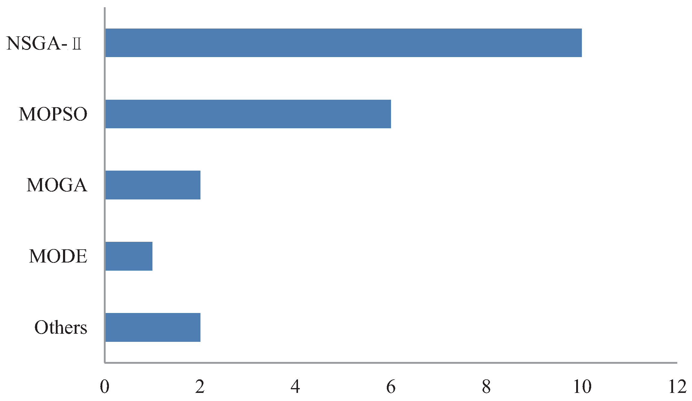
12]. To explore the usage of MOOAs in building performance design, 21 papers using different MOOAs are investigated.
Figure 1 reveals that four algorithms, NSGA-II, MOPSO, MOGA and MODE, are most used for building performance design. Among them, the usage of NSGA-II and MOPSO accounts for 76% of the total 21 papers.
3. Optimization Framework Based on Data Interactive Mechanism and MATLAB
Although numerous optimization tools have been widely applied, researchers and practitioners who are more familiar with MATLAB may wish to use it directly. In this study, we design a MATLAB-based optimization framework to facilitate the algorithms’ realization and comparison.
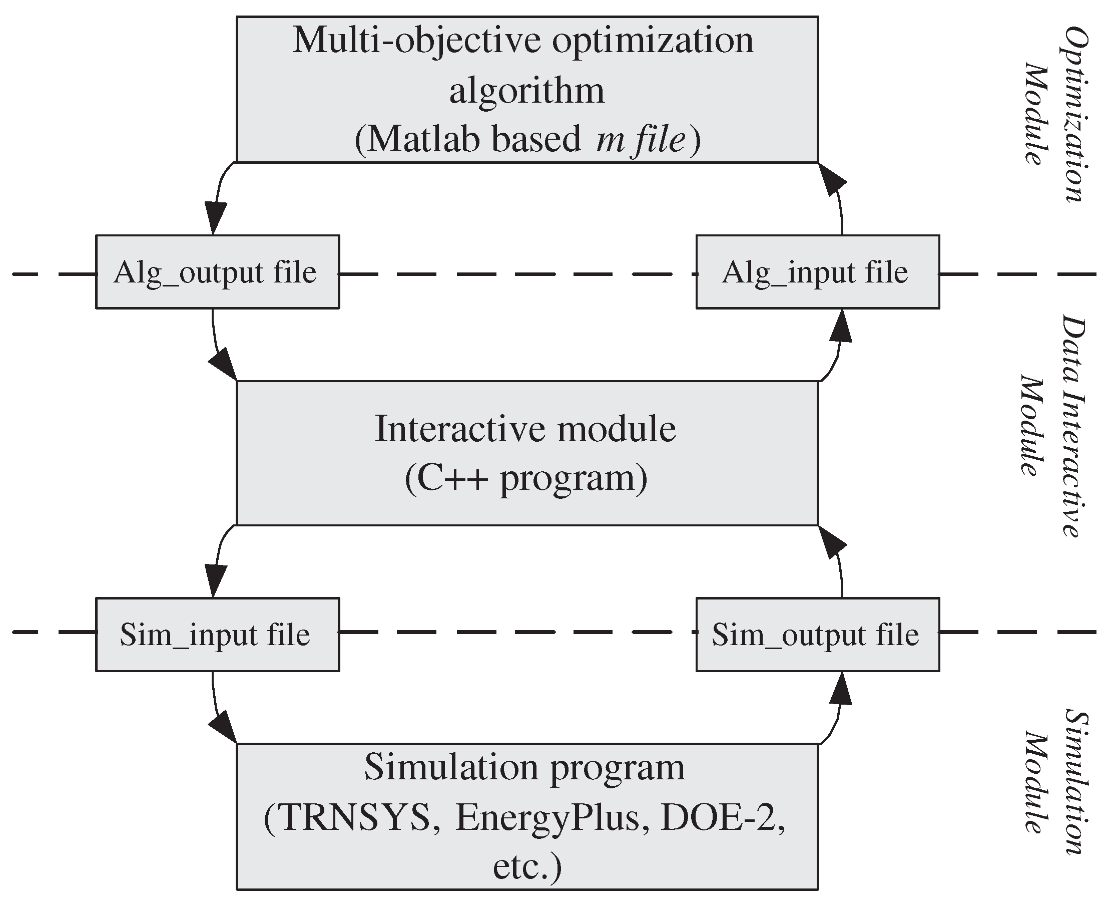
3.1. Data Interactive Mechanism
The proposed optimization framework contains three modules: simulation module (TRNSYS, EnergyPlus, DOE-2, etc.), optimization module (MATLAB) and data interactive module. The key one is a C++-based data interactive module, which interfaces with both the simulation software and MATLAB. The core idea of the data interactive mechanism is: at the beginning of each iteration during the searching procedure, the data interactive module reads control variables from MATLAB, passes them to the simulation software and calls the simulation program. At the end of each iteration, the data interactive module reads the results from the simulation software and passes them to MATLAB to help evaluate the cost function. The basic structure is shown in
Figure 2, along with how it passes data by text files.
A general optimization problem using the proposed data interactive mechanism can be set up as follows:
S1. Build the whole building energy simulation using mature software, such as TRNSYS, EnergyPlus and DOE-2. Make sure that the simulation program reads the control variables and writes the related results by text files.
S2. Define objective function(s), specify possible constraints on the control variables and apply an optimization algorithm in MATLAB in the form of . Make sure that the objective function(s) is evaluated by writing and reading properly at each iteration.
S3. Specify all of the IO files properly in the interactive module, and run the optimization by calling the optimization.
S4. Read the optimized control variables in MATLAB when the stopping criterion is satisfied.
3.2. Multi-Objective Optimization Algorithms
MOOAs are based on Pareto-dominance, which enables the algorithm to optimize all of the objectives simultaneously. They can overcome many shortcomings of the classical weighted-sum approach, as well as providing more solutions from a single optimization problem. Four multi-objective optimization algorithms are briefly described below. They are all applied using the proposed framework and compared in
Section 5.
3.2.1. NSGA-II
Being a population-based approach, GA are well suited to solve multi-objective optimization problems. The NSGA-II is one of the most commonly-used MOOAs [
33]. As a modified version of NSGA, NSGA-II has a better sorting algorithm, incorporates elitism, and no sharing parameter needs to be chosen. At each generation, the populations are combined and sorted according to the non-domination concept. The number of non-dominated points available after sorting may be greater than the populations size
N, which defines the number of elite points that are kept by the algorithm. The algorithm selects the
N least crowded solutions by using the crowding distance measure and rejects the rest of the non-dominated points. Due to these improvements, both convergence and spreading of the solution front are ensured, without requiring the use of any external population [
37].
3.2.2. MOPSO
Moore and Chapman firstly proposed the feasibility PSO algorithm in solving multi-objective optimization problems [
38]. MOPSO is characterized by the excellent maneuverability and convergence, which has been validated and applied widely by many researchers. Each potential solution, which is called a particle, is compared to a flying bird within the search space. Each particle is characterized by its position, velocity and past performance. The particles fly randomly and update themselves by their own characteristic and social characteristics from other particle. There is an extra set called the external archive containing all of the particle leaders. Archive will be updated at each iteration when the new leader particle is better than the old one. Finally, the external archive contains the output of the searching results [
36].
3.2.3. MOGA
There are many variations of multi-objective GA in the literature. In this study, we use MATLAB’s ‘gamultiobj’ function (a variant of NSGA-II) for comparison. Like any other GA, it is based on the evolution of a population of individuals, each of which is a solution to the optimization problem.
3.2.4. MODE
Differential evolution (DE) is a branch of evolutionary algorithms developed by Rainer Storn and Kenneth Price [
39]. The approach works by creating a random initial population of potential solutions where it is guaranteed by some repair rules. In MODE, an initial population is generated at random from a Gaussian distribution; all dominated solutions are removed from the population; if the number of non-dominated solutions exceeds some threshold, a distance metric relation is used to remove those parents who are very close to each other. Three parents are selected at random. A child is generated from the three parents and is placed into the population if it dominates the first selected parent; otherwise, a new selection process takes place. This process continues until the population is completed.
4. Investigation of Different Optimization Strategies: Case Study I
A simple structure containing three thermal zones is constructed in this section. The proposed optimization framework with other two strategies, the GenOpt method and the ANN method, are all employed for performance comparison.
4.1. Model Description
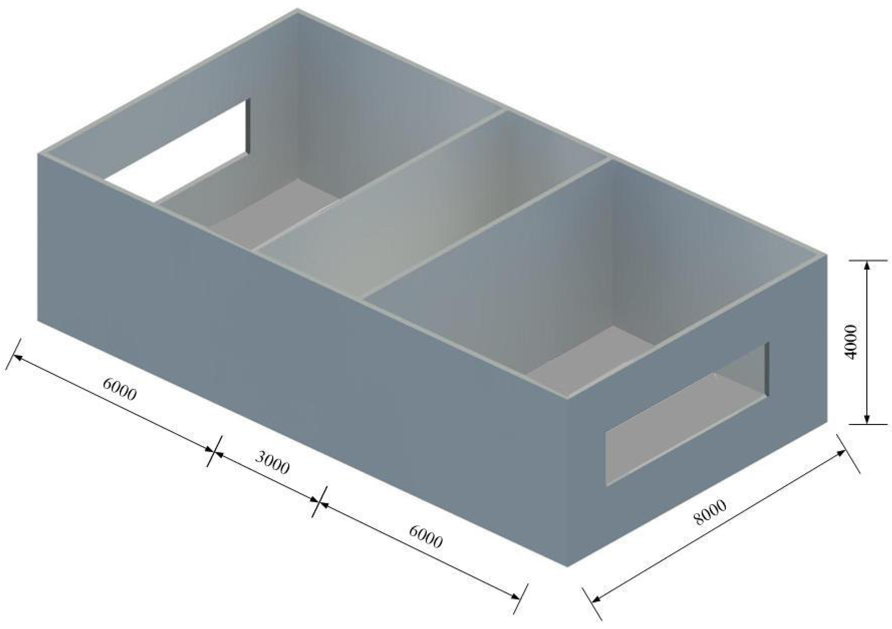
The simple model is shown in
Figure 3 referring to the literature [
29]. The structure (length × width = 7.4 m × 4.1 m) is divided into three rooms: a north-facing room, a south-facing room and a hallway between the two rooms. The walls are made of concrete and have 20 cm of exterior insulation. Both windows have an external shading device that is activated only during summer when the total solar irradiation on the window exceeds 200 W/m
.
4.2. Objective Function and Design Variables
For simplicity, a single objective of annual energy consumption is set in this case study, which is expressed as:
where
and
are the zone’s annual heating and cooling load (kWh) respectively;
and
are the zone’s primary electricity consumption (kWh) for lighting and electrical appliance, respectively;
and
are plant efficiencies that relate the zone load to the primary energy consumption for heating and cooling generation, including electricity consumption for fans and pumps.
Three design variables are chosen to be optimized: the width of both windows, the transmittance of the external shading device and the azimuth of the whole building. These three variables are proven to have impacts on annual energy consumption [
40,
41]. The ranges of design variables are summarized in
Table 1.
4.3. Performance Comparison
We build the structure model using EnergyPlus. Four variables
,
,
and
are set as the output of EnergyPlus. For the proposed optimization framework, we set the interactive module as
Section 3’s description. At the beginning of each iteration, the new values of the design variables are updated to the model file of EnergyPlus by the interactive module; at the end of each iteration, the outputs of the simulation are automatically saved to report files, which will be read by the interactive module for objectives’ evaluation in MATLAB. For GenOpt method, the optimization design is similar to the literature [
21,
32]. For the ANN method, a three-layer feed-forward neural network with input, hidden and output layers, is setup for surrogate model construction. The network training and validation refers to [
12]. Here, we provide the ANN’s basic setup in
Table 2. The same PSO algorithm is implemented in MATLAB and GenOpt. The details of the parameters’ setting are shown in
Table 3. Two criteria are selected for comparison: execution time and optimal searching ability. All simulations are carried out using the same workstation with 3.4-GHz quad-core processors and 8 G RAM.
To investigate each approach’s performance, all three strategies conduct twelve optimization runs. The best five results are recorded in
Table 4 and
Table 5. It can be seen from
Table 4 that the ANN method has the shortest execution time (less than 1 min). It should be noted that the training time for ANN modeling is not included (costs extra 70 min or so). The proposed framework has a similar execution time compared with GenOpt (shortens average execution time by 5.4%).
Table 5 shows that GenOpt and the proposed framework achieve similar optimal solutions. This means that the proposed framework has competitive performances compared with the GenOpt method. Additionally, the MATLAB interface gives it great potential in complex building performance optimization applications. For the ANN method, the optimization performance is largely dependent on the modeling accuracy. In this case, the optimal solution is worse than the other two strategies. The modeling error is the main reason [
24].
5. Optimization Algorithms Comparison: Case Study II
We have validated the performance of the proposed method using Case Study I. Here, a more practical and complicated case is modeled for optimization algorithms’ investigation. With the aid of the MATLAB interface, four multi-objective algorithms, NSGA-II, MOPSO, MOGA and MODE, are realized and compared.
5.1. Model Description
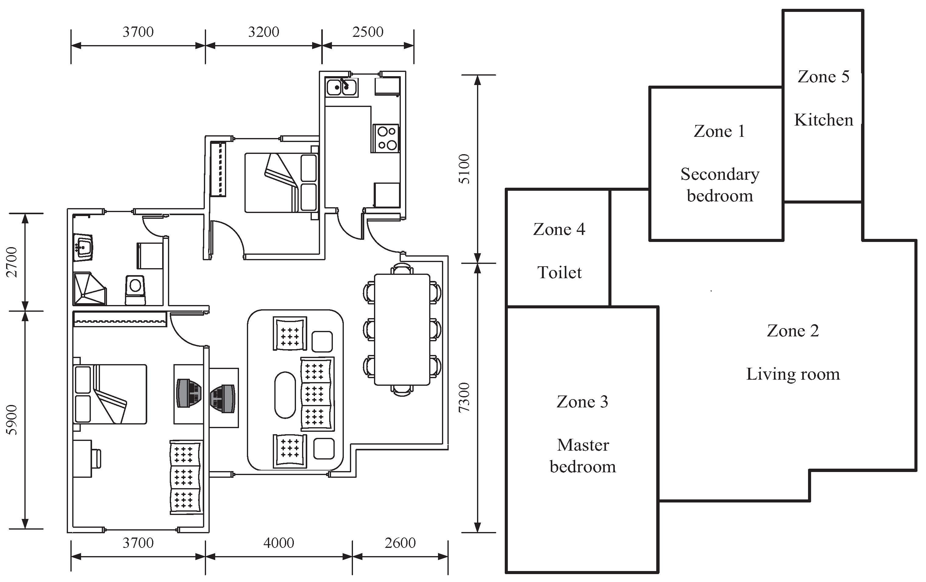
A typical residential building located in Nanjing, East China, is chosen for the second case study. The structure of the building is shown in
Figure 4 (left). The gross floor area is 104 m
, and its floor-to-roof height is 3 m. Detailed information about the geometry and layout of the residential building is listed in
Table 6. In order to facilitate the consumption calculation, the house is divided into five thermal zones (shown in
Figure 4 (right)). It is assumed that the building is equipped with variable refrigerant volume (VRV) air conditioning systems in the master bedroom, secondary bedroom and living room. The heating and cooling set points are
and
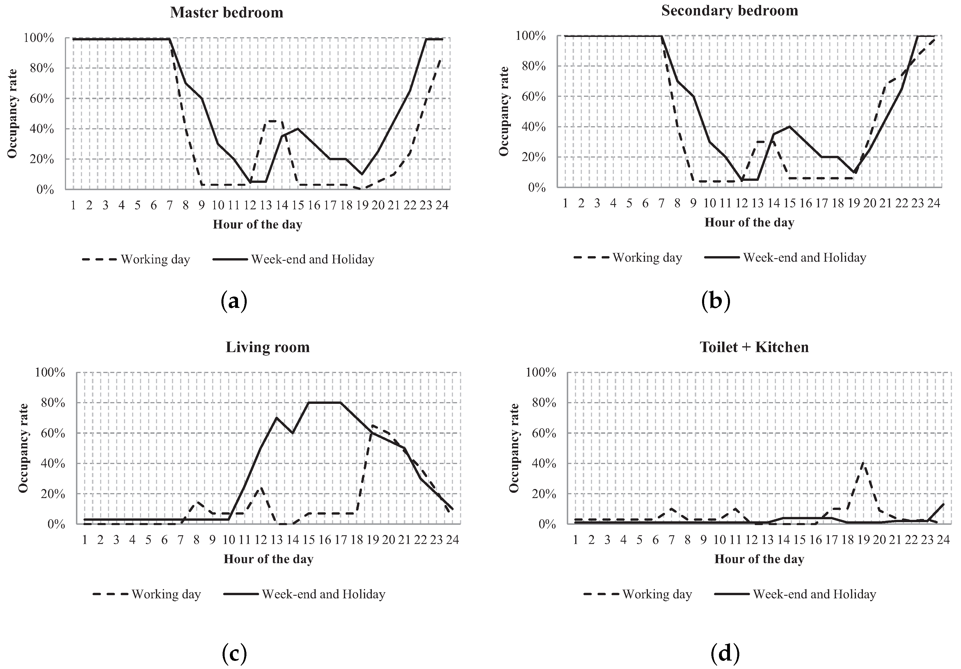
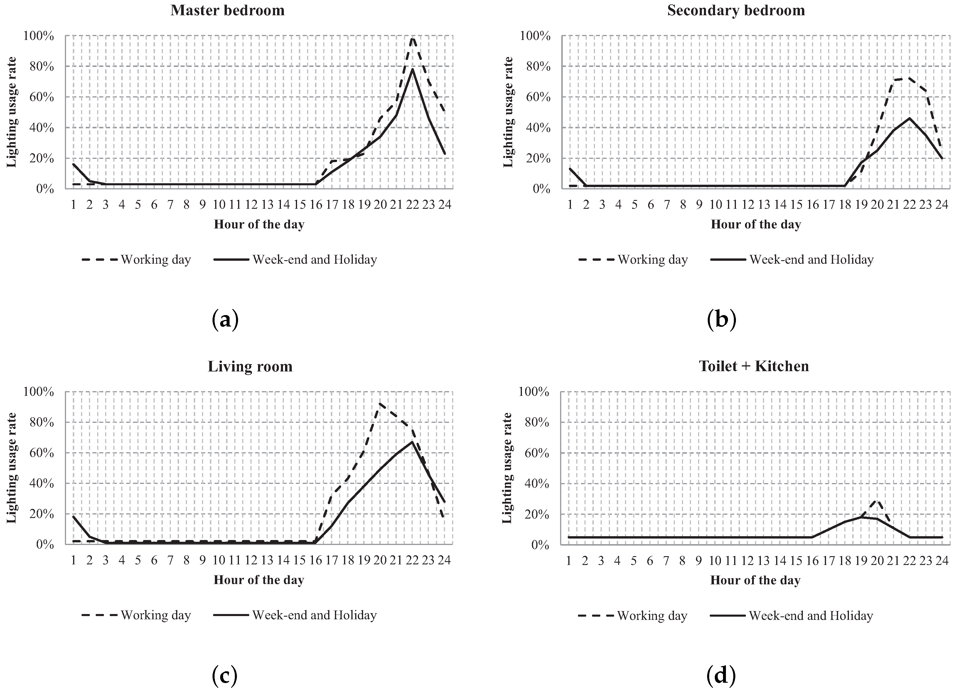
for the operating strategy of the zone thermostat control. Each zone is equipped with a fluorescent lamp (CFL) lighting system. The occupancy, total residential lights and electric equipment loads are recorded and adjusted at each time step. Details are shown in
Figure A1,
Figure A2 and
Figure A3 and
Table A1. Air infiltration is assumed only for the kitchen and toilet at the rate of 0.002 m
s. We assume that the life cycle of the residential building is 30 years.
5.2. Design Variables and Objective Functions
In this case, 16 building performance-related parameters are considered as design variables. As we know, envelop-related variables are commonly defined as continuous variables to facilitate the optimization [
42], such as conductivity, thermal absorbance, visible absorbance, etc. However, the optimum results may not be obtained for sure in a practical application, because real materials probably do not match the optimum ones exactly [
43]. In this study, all of the material component variables are treated as discrete variables, and only materials, which are available on the market (recorded in
Table A2), are used in the optimization process. Beyond that, the window-to-wall ratio (WWR) of three zones and the azimuth are set as continuous variables.
Table 7 shows all of the design variables with the corresponding range of variation.
With the consideration of economic demand, environmental issues and thermal comfort simultaneously, three indicators are set as objectives for the optimization application. They are the life cycle cost (LCC), the carbon dioxide equivalent (CO) and the total percentage of cumulative time with discomfort over the whole year (TPMVD).
(1) LCC:
Building LCC includes all of the costs during the building’s lifespan. LCC provides a comprehensive and consistent evaluation for discerning the true economic benefits of the building [
44]. Generally, the indicator is formulated as the following equation [
45]:
where
represents the initial costs,
represents the total operation cost,
represents the repair and maintenance cost during the life cycle and
represents recycle and disposal cost in the end. Operation cost mainly includes annual electrical energy consumption. Considering the global energy shortage, as well as currency devaluation, operation cost takes the inflation and escalation in energy prices into consideration.
(2) CO:
CO
emission in the residential buildings is classified into material production CO
emission and operation CO
emission. Material production
emission is the sum of the CO
emission when construction materials are produced and transported. Operation CO
emission mainly includes the emission of electricity consumption in the building. To determine the electricity-related emissions, the annual heating and cooling load is calculated first [
36]. The total CO
emission during the life cycle is expressed as:
where
m is the number of the building materials;
is the CO
emission of the
i-th material (kg/m
);
is the area of the
i-th material (m
);
t is the the whole life cycle (years);
is the electricity CO
emission (kg/kWh);
is the annual electricity consumption of the building (kWh). The CO
emissions of the building materials used in this study are recorded in
Table A3.
(3) TPMVD:
As we know, index PMV assesses thermal comfort level by a function of four environmental variables (temperature, relative humidity, mean radiant temperature and air velocity) and two individual parameters (metabolic rate and clothing value). The PMV value of zero is expected to provide the lowest percent of people dissatisfied (PPD) among a population [
46]. In order to adjust the thermal comfort, the total percentage of cumulative time with discomfort over the whole year during the occupancy period is evaluated as TPMVD. It is a two-tailed index that measures the thermal discomfort throughout the whole year. The index of TPMVD can be expressed as [
12]:
where
and
represent the borders of the thermal comfort and
is the index PMV at each time step.
5.3. Criteria for Performance Comparison
In this case, four different multi-objective optimization algorithms are applied. The performance of each algorithm is evaluated in three aspects [
34]:
(1) Execution time;
(2) Convergence to the optimal set, indicated by the normalized generational distance, ;
(3) Diversity of solutions in the Pareto-optimal set, indicated by the normalized diversity metric, .
To avoid the biases to one objective function, the
and
are calculated on the optimal solutions by using the normalized values of the three objective functions (denoted by Xn, Yn and Zn). Xn, Yn and Zn are described as follows:
The
indicates the average Euclidean distance between the best Pareto front and the optimal solution obtained by each algorithm. The convergence metric can be expressed as follows:
where
is the Euclidean distance between the obtained solution and the nearest best Pareto solutions.
n is the number of obtained solutions.
The normalized diversity metric
is used to measure the diversity of the obtained solutions. It is calculated as:
where
is the Euclidean distance between the consecutive solutions in the obtained non-dominated set of solutions;
is the average of
assuming there are
N solutions in the obtained non-dominated set;
and
are the Euclidean distances between the extreme and the boundary solutions. By definitions, lower values of
and
are both preferred.
5.4. Algorithm Performance Comparison
With the aid of the MATLAB interface, four popular multi-objective algorithms, NSGA-II, MOPSO, MOGA and MODE, are realized in the proposed framework. The parameters’ settings are important, affecting the optimization performance. For different kinds of algorithms, it is hard to adjust every parameter equally. Here, population size and the iteration number of each algorithm are both set to the same values. For the other parameters, we set the default values. The parameter settings are shown in
Table 8. Based on the framework described in
Section 3, the optimization case is set up using the proposed data interactive mechanism. All experimental settings are identical to Case I. Three objective functions are defined according to
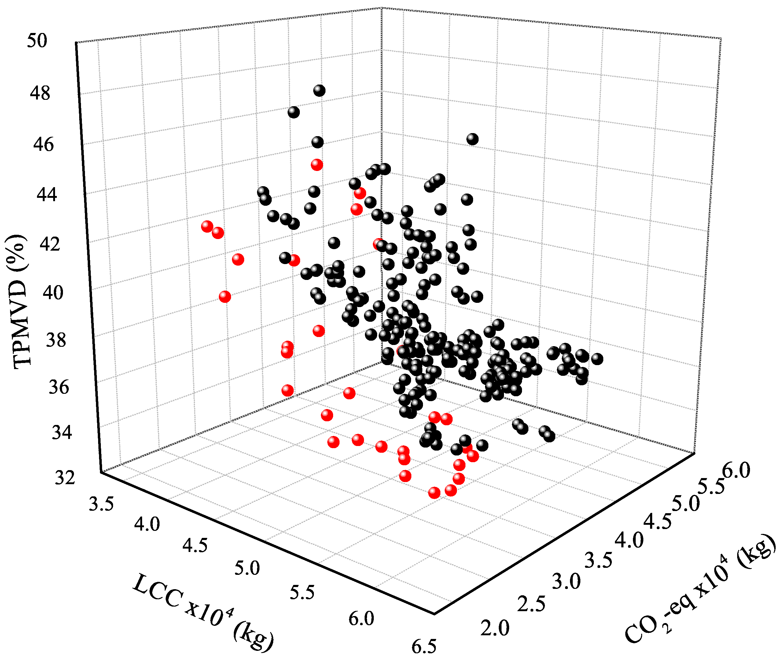
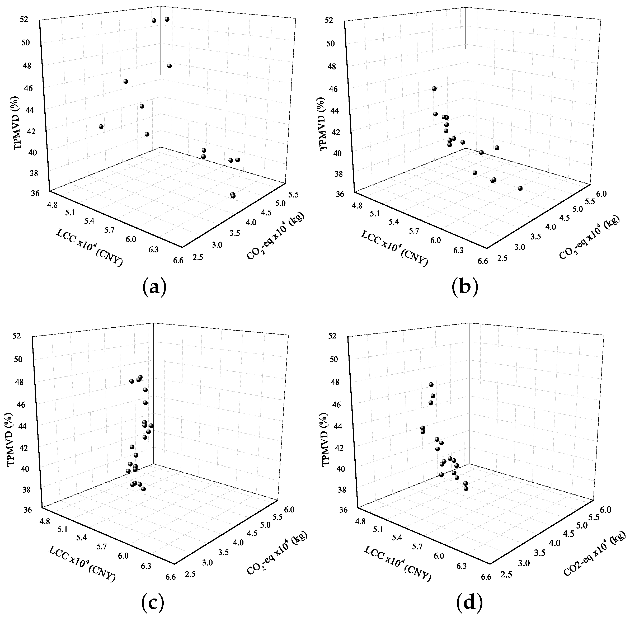
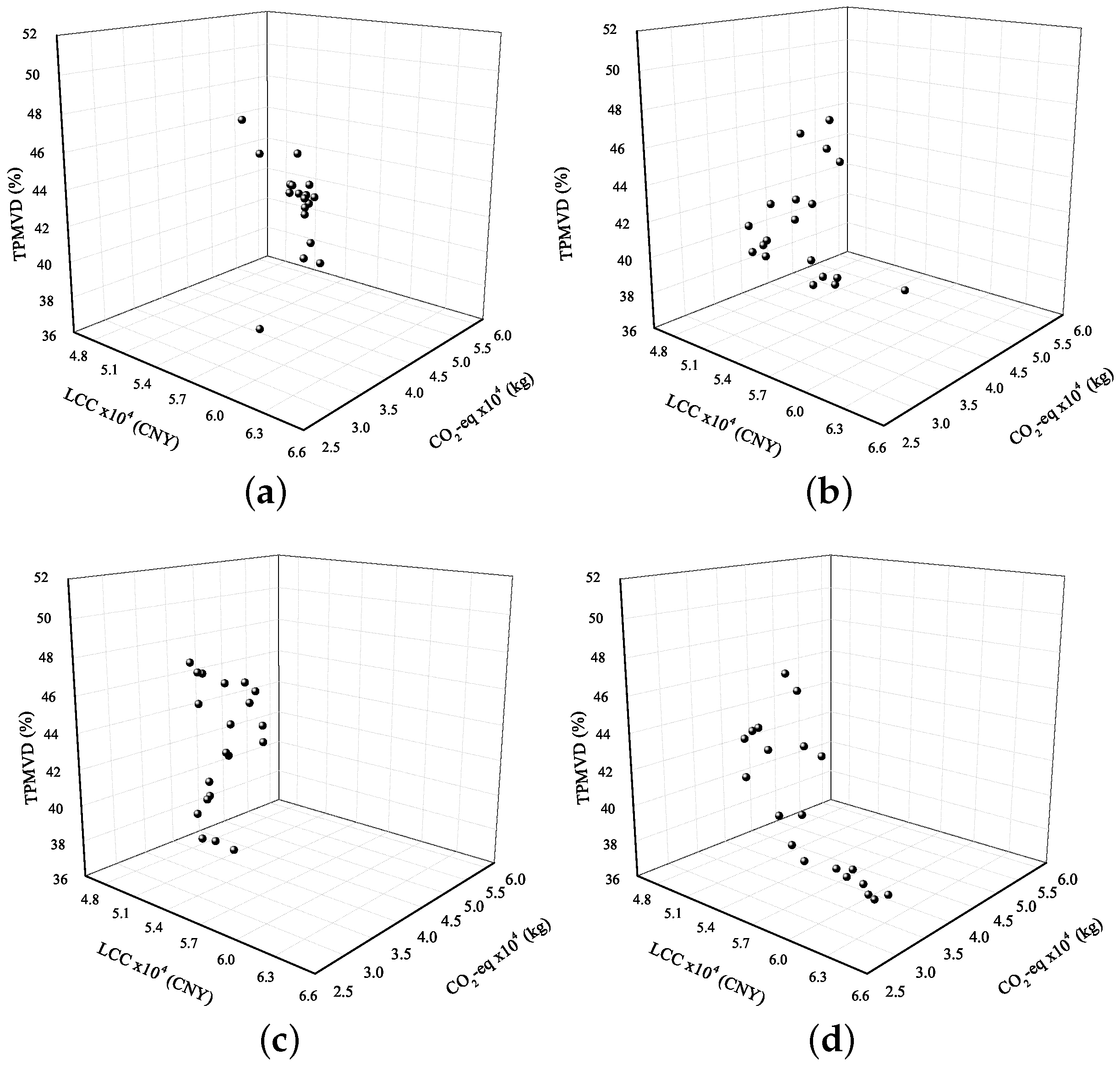
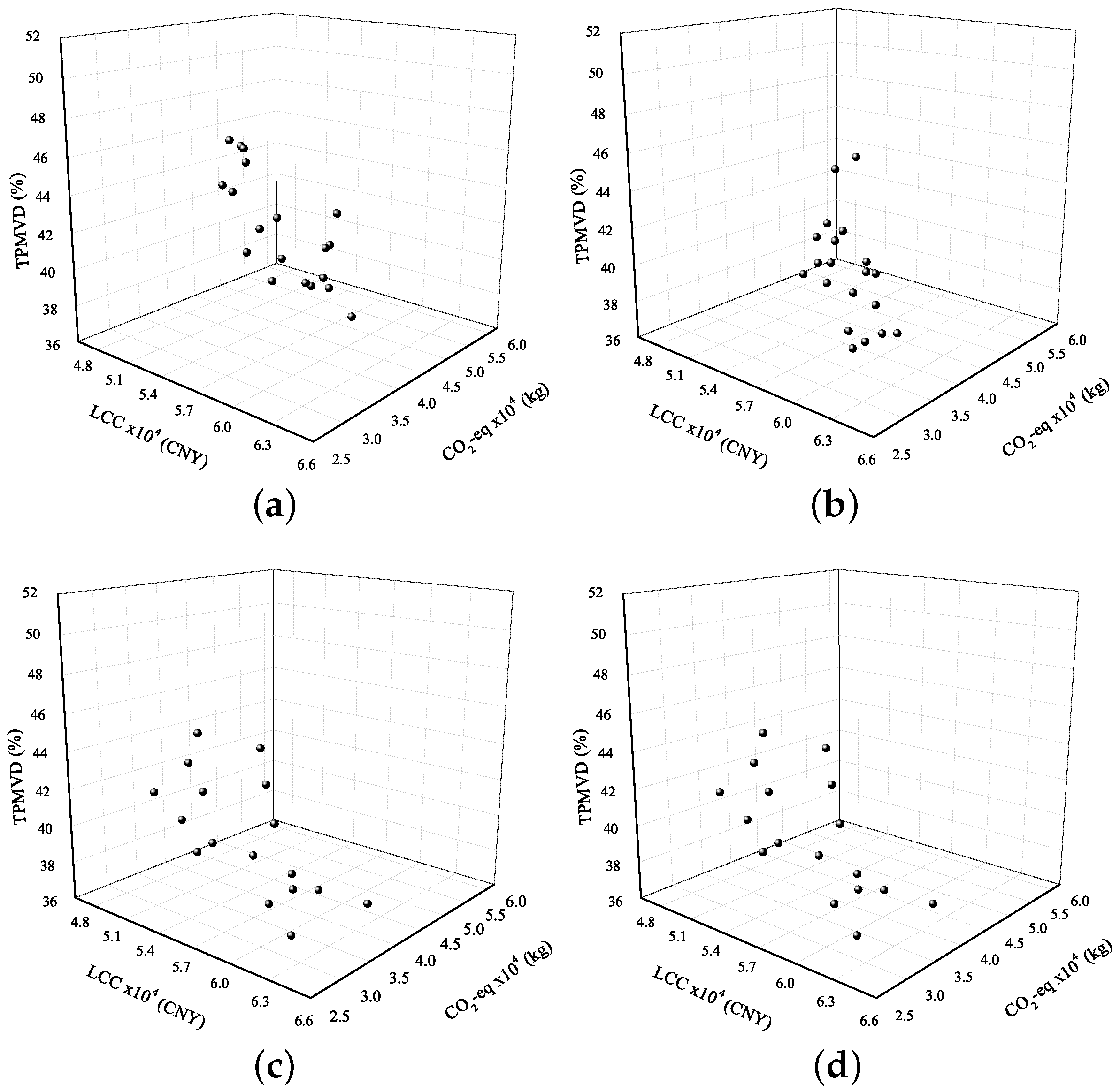
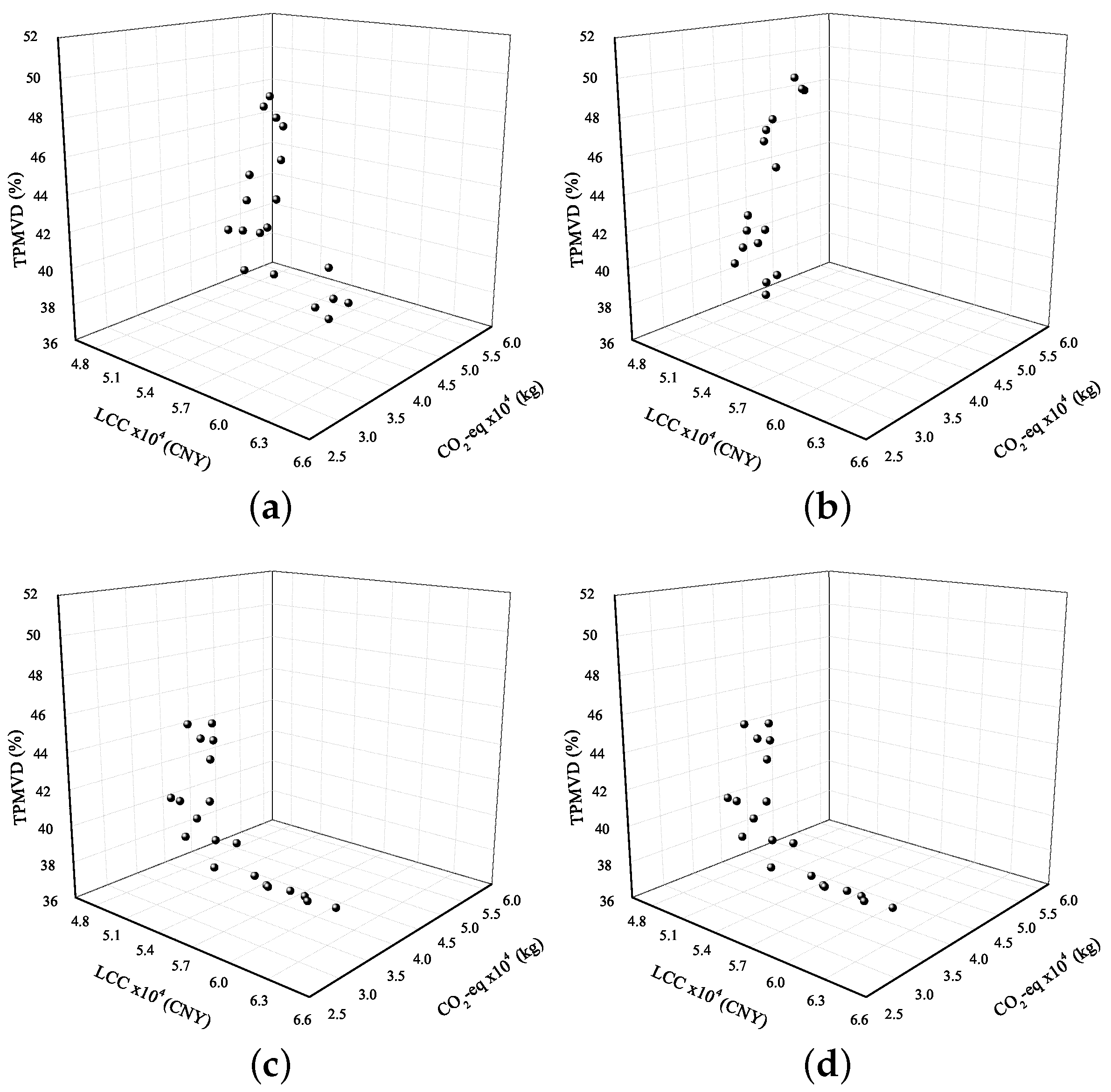
Section 5.2’s discussion. Each algorithm is executed five times. In order to evaluate the convergence procedure of each algorithm, we record their Pareto frontiers at 30, 60, 90 and 120 generations, respectively, in
Figure 6,
Figure 7,
Figure 8 and
Figure 9. All of the obtained Pareto solutions are collected in
Figure 5. In this figure, the red points represent the best Pareto solutions finally obtained by all four algorithms.
From
Figure 6,
Figure 7,
Figure 8 and
Figure 9, it can be seen that after 120 generations, NSGA-II, MOGA and MODE all almost achieve their steady states.
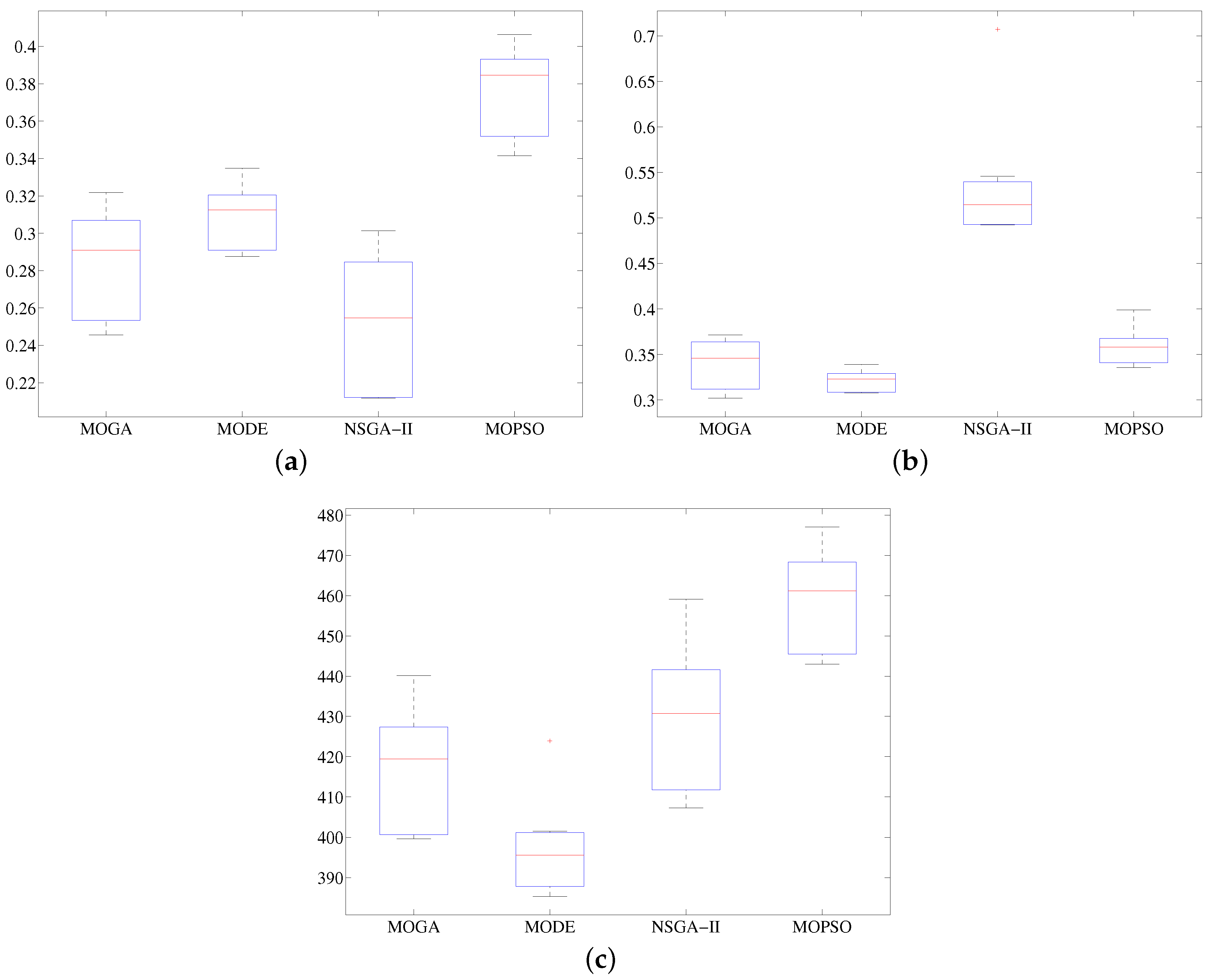
Table 9 shows that NSGA-II and MOGA have the similar best execution time (400 min or so). MODE coverages most quickly and takes about 90 generations to complete the whole optimization procedure. The execution time of MODE ranges from 385 min–423 min, and the best time is only 385 min. Comparatively speaking, MOPSO costs the longest time to reach convergence (442 min–477 min).
In terms of convergence of the obtained solutions (indicated by the GDn), the NSGA-II obtains a better average/best GDn (0.25 and 0.21) than the others, while the MOPSO is still the worst (average: 0.38; and best: 0.34).
In terms of the diversity of the obtained solutions (indicated by the
), MODE, MOGA and MOPSO have similar performances. Compared with them, the diversity of NSGA-II performs poorly. From
Figure 6, it is seen that Pareto solutions of NSGA-II are tightly clustered near the best Pareto solutions. The average
DMn of NSGA-II is 0.54582. The boxplots of the three indexes for four algorithms are also provided in
Figure 10.
In general, MODE outperforms the others in two of three indicators, including execution time and . It shows MODE’s competitive ability for building performance optimization. In this case, MOPSO does not exhibit any outstanding features. MOGA and NSGA-II achieve average rankings in most tests; thus, they can be trusted to find a near optimal design solution. It is worth noting that an algorithm may achieve high performance on one criterion, but obtain low performance on other criteria. Hence, it is hard to draw any solid conclusions from the single case study.
5.5. Result Analysis
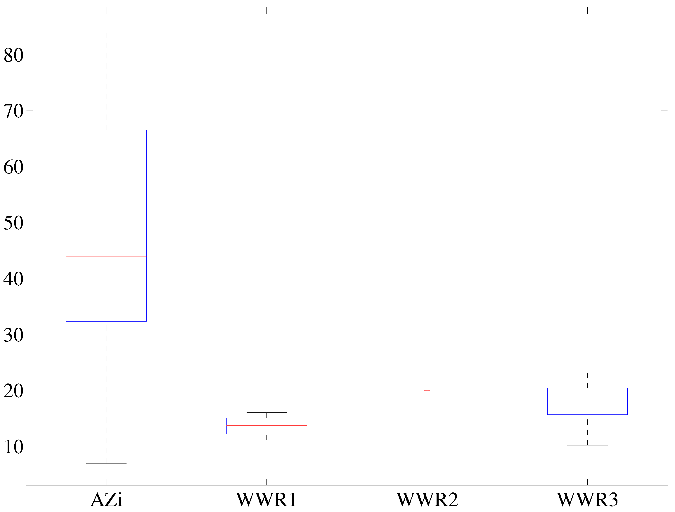
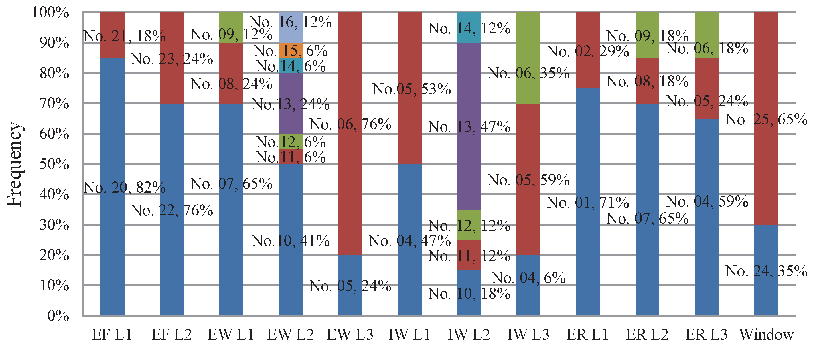
Figure 11 and
Figure 12 show the dispersion of the building parameters on the best Pareto frontier, which may help designers make decisions on building performance design. For example, by examining the design parameters on the best Pareto frontier, it is evident that 100-mm concrete (Material No. 20; see
Table A2) and carpet (Material No. 22) are the most used in the construction of the floor. For exterior walls and windows, frequently-used materials corresponding to the best solutions can also be found. It is worthwhile to mention that some of building envelope components have non-dominated solutions. The reason is that the economic and environmental costs are conflicting in reality. The prices of environmentally-friendly materials are commonly higher than those of conventional ones. However, if the thermal performance of the building is poor, the energy consumption of the HVAC system will increase. Hence, the improvement of thermal comfort performance at the building design phase can cut the energy consumption of the HVAC system in the operation phase.
6. Conclusions
In this paper, a MATLAB-based interactive optimization framework is developed to facilitate building performance optimization designs. A performance comparison of three optimization schemes, including the GenOpt, ANN and the proposed method, has been carried out by means of computational experiments using a simple building energy model. Results show that the ANN method has the shortest execution time, but the modeling error makes its optimization solution poor. Relatively, the proposed interactive framework has competitive performances compared with the GenOpt method, and its MATLAB interface makes it suitable for applying latest algorithms for complex building performance optimizations.
With the proposed optimization platform, the comparison of four popular multi-objective optimization algorithms, including the NSGA-II, MOPSO, MOGA and MODE, has been carried out using a practical project located in Nanjing, China. To quantify the main features of these MOOAs, three criteria are applied along with a comprehensive test procedure. Two important assumptions of this case study are that (i) all algorithms have the same generation/population sizes and (ii) other settings of the algorithms are set as default. Results show that MODE is superior to the others in the indicators of execution time and . MOGA and NSGA-II achieve average rankings in most tests. MOPSO does not exhibit any outstanding features in this case. The performance of the MOOAs may be sensitive to different cases; more criteria and case studies will be conducted in the future work.
Acknowledgments
This work is supported by National Natural Science Foundation of China (Grant No. 61304075, 61233006), the Jiangsu Provincial Natural Science Foundation of China (Grant No. BK20150525), the China Postdoctoral Science Foundation (Grant No. 2016M601741, 2016M591784, 2016M600381) and the Jiangsu Provincial Postdoctoral Science Foundation of China (Grant No. 1601130B, 1501101B, 1601038C).
Author Contributions
Kangji Li designed the optimization framework. Lei Pan developed the interactive module and performed the case studies. Wenping Xue and Hui Jiang realized all of the algorithms. Hanping Mao gave advice on framework design and paper structure. Lei Pan wrote the paper.
Conflicts of Interest
The authors declare no conflict of interest.
Abbreviations
The following abbreviations are used in this manuscript:
| Annual heating load (kWh) |
| Annual cooling load (kWh) |
| Plant efficiency to primary heating consumption |
| Plant efficiency to primary cooling consumption |
| Annual lighting consumption(kWh) |
| Annual electrical consumption(kWh) |
| LCC | Life cycle cost (CNY) |
| IC | Building initial cost (CNY) |
| IE | Building total operation cost (CNY) |
| IR | Building Repair and maintenance cost (CNY) |
| ID | Building recycle and disposal cost (CNY) |
| CO | Carbon dioxide equivalent (kg) |
| Material CO-eq emission (kg/m) |
| Material area (m) |
| Electricity CO-eq emission (kg/kWh) |
| Annual Electricity consumption (kWh) |
| Normalized generational distance |
| Normalized diversity metric |
Appendix A
Table A1.
Maximum predicted occupation and installed electric power within each zone.
Table A1.
Maximum predicted occupation and installed electric power within each zone.
| Zone Name | Net Floor Area (m2) | Number of People | Lighting Power (W) | Electrical Equipment Power (W) |
|---|
Master bedroom
(Zone 1) | 22.55 | 2 | 65 | 200 |
Secondary bedroom
(Zone 2) | 20.87 | 1 | 60 | 175 |
living room
(Zone 3) | 41.26 | 3 | 110 | 500 |
Kitchen+Toilet
(Zone 4 + Zone 5) | 16.32 | 1 | 40 | 1300 |
Table A2.
Reference materials of the building envelope and corresponding cost [
45,
47,
48].
Table A2.
Reference materials of the building envelope and corresponding cost [45,47,48].
| Material No. | Material | Thickness (mm) | Price (CNY/Unit) |
|---|
| 1 | Asphalt shingle | 10 | 35/m |
| 2 | Wood shingle | 2.5 | 38/m |
| 3 | Metal surface | 0.8 | 95/m |
| 4 | Gypsum board | 16 | 15.9/m |
| 5 | Gypsum board | 13 | 11.9/m |
| 6 | Gypsum board | 9.5 | 7.9/m |
| 7 | Fibrous insulation | 10 | 7.8/m |
| 8 | Fibrous insulation | 15 | 11.6/m |
| 9 | Fibrous insulation | 20 | 15.6/m |
| 10 | Cellular polyurethane | 40 | 38/m |
| 11 | Cellular polyurethane | 60 | 57/m |
| 12 | Cellular polyurethane | 80 | 76/m |
| 13 | Rigid insulation fiberglass | 40 | 18/m |
| 14 | Rigid insulation fiberglass | 60 | 28/m |
| 15 | Rigid insulation fiberglass | 80 | 38/m |
| 16 | Brick | 90 | 1.68/Block |
| 17 | Brick | 140 | 2.08/Block |
| 18 | Brick | 190 | 2.58/Block |
| 19 | Concrete | 50 | 305/m |
| 20 | Concrete | 100 | 305/m |
| 21 | Concrete | 150 | 305/m |
| 22 | Carpet | 20 | 16.2/m |
| 23 | Acoustic tile | 9 | 17.1/m |
| 24 | Aluminum window | 6 + 9A + 6 | 19/m |
| 25 | Aluminum window | 8 + 9A + 8 | 27/m |
| 26 | Aluminum window | 10 + 9A + 10 | 43/m |
Table A3.
Total CO emission the building materials used in this study.
Table A3.
Total CO emission the building materials used in this study.
| Material | Unit | CO (kg) |
|---|
| Asphalt shingle | T | 65.44 |
| Wood shingle | m | 5.75 |
| Metal Ferrum | T | 982.16 |
| Gypsum board-16 mm | m | 357 |
| Gypsum board-13 mm | m | 2.14 |
| Gypsum board-9 mm | m | 1.99 |
| Fibrous insulation | T | 2593.14 |
| Cellular polyurethane | T | 1505.89 |
| Rigid insulation fiberglass | T | 2593.14 |
| Brick | m | 473.5 |
| Concrete-2500psi | m | 235.89 |
| Carpet | m | 0.89 |
| Acoustic tile | m | 1.16 |
| Aluminum window-6 mm | m | 20.15 |
| Aluminum window-8 mm | m | 25.51 |
| Aluminum window-10 mm | m | 29.08 |
Figure A1.
Daily schedule for occupancy, (a) Master bedroom; (b) Secondary bedroom; (c) Living room; (d) Toilet and Kitchen.
Figure A1.
Daily schedule for occupancy, (a) Master bedroom; (b) Secondary bedroom; (c) Living room; (d) Toilet and Kitchen.
Figure A2.
Daily schedule for lighting. (a) Master bedroom; (b) Secondary bedroom; (c) Living room; (d) Toilet and Kitchen.
Figure A2.
Daily schedule for lighting. (a) Master bedroom; (b) Secondary bedroom; (c) Living room; (d) Toilet and Kitchen.
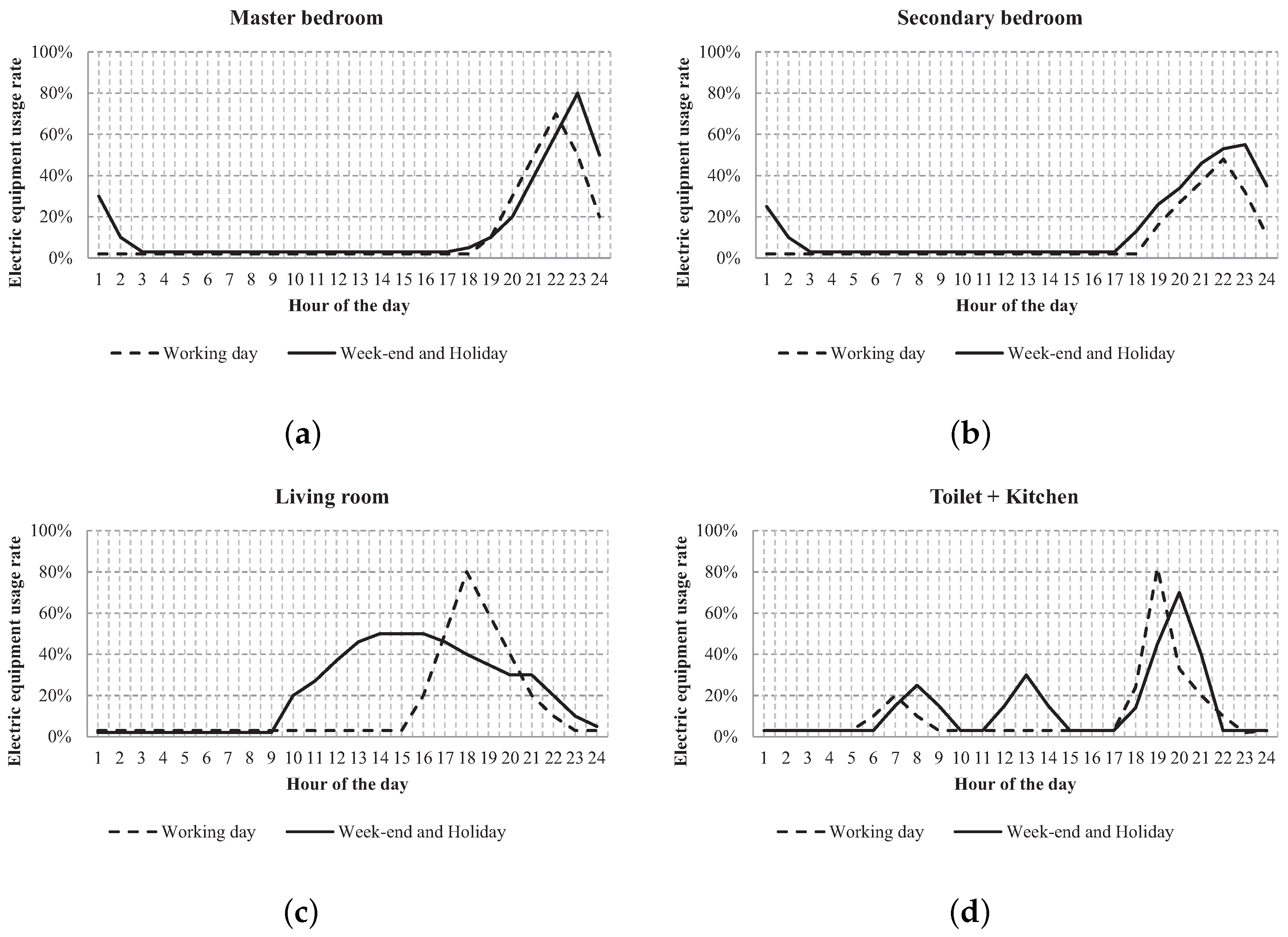
Figure A3.
Daily schedule for electrical equipment. (a) Master bedroom; (b) Secondary bedroom; (c) Living room; (d) Toilet and Kitchen.
Figure A3.
Daily schedule for electrical equipment. (a) Master bedroom; (b) Secondary bedroom; (c) Living room; (d) Toilet and Kitchen.
References
- Boeck, L.D.; Verbeke, S.; Audenaert, A.; Mesmaeker, L.D. Improving the energy performance of residential buildings: A literature review. Renew. Sustain. Energy Rev. 2015, 52, 960–975. [Google Scholar] [CrossRef]
- Maraseni, T.N.; Maroulis, G.C.J. An assessment of greenhouse gas emissions: Implications for the Australian cotton industry. J. Agric. Sci. 2010, 148, 501–510. [Google Scholar] [CrossRef]
- Khanna, N.; Zhou, N.; Ke, J.; Fridley, D. Evaluation of the Contribution of the Building Sector to PM2.5 Emissions in China. J. Biol. Chem. 2014, 87, 767–784. [Google Scholar]
- Nejat, P.; Jomehzadeh, F.; Taheri, M.M.; Gohari, M.; Majid, M.Z.A. A global review of energy consumption, CO2 emissions and policy in the residential sector (with an overview of the top ten CO2 emitting countries). Renew. Sustain. Energy Rev. 2015, 43, 843–862. [Google Scholar] [CrossRef]
- Li, D.H.; Yang, L.; Lam, J.C. Zero energy buildings and sustainable development implications. A review. Energy 2013, 54, 1–10. [Google Scholar] [CrossRef]
- Hamdy, M.; Hasan, A.; Kai, S. A multi-stage optimization method for cost-optimal and nearly-zero-energy building solutions in line with the EPBD-recast 2010. Energy Build. 2013, 56, 189–203. [Google Scholar] [CrossRef]
- Sinha, D. Design of an Energy Efficient Building via Multivariate Stochastic Optimization. Master’s Thesis, University of Florida, Gainesville, FL, USA, 2012. [Google Scholar]
- Rojas, J.M.; Galan Marin, C.; Fernandez Nieto, E.D. Parametric Study of Thermodynamics in the Mediterranean Courtyard as a Tool for the Design of Eco-Efficient Buildings. Energies 2012, 5, 2381–2403. [Google Scholar] [CrossRef]
- Li, K.; Xue, W.; Liu, G. A general optimization framework for complex PDE models based on data interactive mechanism. In Proceedings of the IEEE International Conference on Advanced Intelligent Mechatronics, Busan, Korea, 7–11 July 2015.
- Machairas, V.; Tsangrassoulis, A.; Axarli, K. Algorithms for optimization of building design: A review. Renew. Sustain. Energy Rev. 2014, 31, 101–112. [Google Scholar] [CrossRef]
- Foucquier, A.; Robert, S.; Suard, F.; Stephan, L.; Jay, A. State of the art in building modelling and energy performances prediction: A review. Renew. Sustain. Energy Rev. 2013, 23, 272–288. [Google Scholar] [CrossRef]
- Asadi, E.; Silva, M.G.D.; Antunes, C.H.; Dias, L.; Glicksman, L. Multi-objective optimization for building retrofit: A model using genetic algorithm and artificial neural network and an application. Energy Build. 2014, 81, 444–456. [Google Scholar] [CrossRef]
- Nguyen, A.T.; Reiter, S.; Rigo, P. A review on simulation-based optimization methods applied to building performance analysis. Appl. Energy 2014, 113, 1043–1058. [Google Scholar] [CrossRef]
- Turner, G. Recorded Commercial Optimization Method and System. U.S. Patent 20080263581 A1, 23 October 2008. [Google Scholar]
- Bucking, S.; Zmeureanu, R.; Athienitis, A. An information driven hybrid evolutionary algorithm for optimal design of a Net Zero Energy House. Solar Energy 2013, 96, 128–139. [Google Scholar] [CrossRef]
- Delgarm, N.; Sajadi, B.; Kowsary, F.; Delgarm, S. Multi-objective optimization of the building energy performance: A simulation-based approach by means of particle swarm optimization (PSO). Appl. Energy 2016, 170, 293–303. [Google Scholar] [CrossRef]
- Chantrelle, F.P.; Lahmidi, H.; Keilholz, W.; Mankibi, M.E.; Michel, P. Development of a multicriteria tool for optimizing the renovation of buildings. Appl. Energy 2011, 88, 1386–1394. [Google Scholar] [CrossRef]
- Futrell, B.J.; Ozelkan, E.C.; Brentrup, D. Optimizing complex building design for annual daylighting performance and evaluation of optimization algorithms. Energy Build. 2015, 92, 234–245. [Google Scholar] [CrossRef]
- Hong, T.; Chen, Y.; Sang, H.L.; Zhang, R.; Sun, K.; Taylor-Lange, S.C.; Piette, M.A.; Price, P.; Kloss, M.; Bourassa, N. Commercial Building Energy Saver: An Energy Retrofit Analysis Toolkit. In Proceedings of the ISHVAC - COBEE, Tianjin, China, 12–15 July 2015; pp. 298–309.
- Chen, Y.; Treado, S. Development of a simulation platform based on dynamic models for HVAC control analysis. Energy Build. 2014, 68, 376–386. [Google Scholar] [CrossRef]
- Karaguzel, O.T.; Zhang, R.; Lam, K.P. Coupling of whole-building energy simulation and multi-dimensional numerical optimization for minimizing the life cycle costs of office buildings. Build. Simul. 2014, 7, 111–121. [Google Scholar] [CrossRef]
- Zhang, F.; Deb, C.; Lee, S.E.; Yang, J.; Shah, K.W. Time series forecasting for building energy consumption using weighted Support Vector Regression with differential evolution optimization technique. Energy Build. 2016, 126, 94–103. [Google Scholar] [CrossRef]
- Gossard, D.; Lartigue, B.; Thellier, F. Multi-objective optimization of a building envelope for thermal performance using Genetic Algorithms and Artificial Neural Network. Energy Build. 2013, 67, 253–260. [Google Scholar] [CrossRef]
- Wei, Y.; Li, B.; Jia, H.; Ming, Z.; Di, W. Application of multi-objective genetic algorithm to optimize energy efficiency and thermal comfort in building design. Energy Build. 2015, 88, 135–143. [Google Scholar]
- Magnier, L.; Haghighat, F. Multiobjective optimization of building design using TRNSYS simulations, genetic algorithm, and Artificial Neural Network. Build. Environ. 2010, 45, 739–746. [Google Scholar] [CrossRef]
- Li, K.; Su, H.; Chu, J.; Xu, C. A fast-POD model for simulation and control of indoor thermal environment of buildings. Build. Environ. 2013, 60, 150–157. [Google Scholar] [CrossRef]
- Lobato, F.S.; Sousa, M.N.; Silva, M.A.; Machado, A.R. Multi-objective optimization and bio-inspired methods applied to machinability of stainless steel. Appl. Soft Comput. 2014, 22, 261–271. [Google Scholar] [CrossRef]
- Eisenhower, B.; Fonoberov, V.A.; Mezic, I. Uncertainty-weighted meta-model optimization in building energy models. In Proceedings of the First Building Simulation and Optimization Conference, Loughborough, UK, 10–11 September 2012.
- Wetter, M.; Polak, E. Building design optimization using a convergent pattern search algorithm with adaptive precision simulations. Energy Build. 2005, 37, 603–612. [Google Scholar] [CrossRef]
- Wetter, M.; Wright, J. A comparison of deterministic and probabilistic optimization algorithms for nonsmooth simulation-based optimization. Build. Environ. 2004, 39, 989–999. [Google Scholar] [CrossRef]
- Almeida, P.; Carvalho, M.J.; Amorim, R.; Mendes, J.F.; Lopes, V. Dynamic testing of systems—Use of TRNSYS as an approach for parameter identification. Solar Energy 2014, 104, 60–70. [Google Scholar] [CrossRef]
- Asadi, E.; Silva, M.G.D.; Antunes, C.H.; Dias, L. A multi-objective optimization model for building retrofit strategies using TRNSYS simulations, GenOpt and MATLAB. Build. Environ. 2012, 56, 370–378. [Google Scholar] [CrossRef]
- Brownlee, A.E.I.; Wright, J.A. Constrained, mixed-integer and multi-objective optimisation of building designs by NSGA-II with fitness approximation. Appl. Soft Comput. 2015, 33, 114–126. [Google Scholar] [CrossRef] [Green Version]
- Hamdy, M.; Nguyen, A.T.; Hensen, J.L. A performance comparison of multi-objective optimization algorithms for solving nearly-zero-energy-building design problems. Energy Build. 2016, 121, 57–71. [Google Scholar] [CrossRef]
- Karmellos, M.; Kiprakis, A.; Mavrotas, G. A multi-objective approach for optimal prioritization of energy efficiency measures in buildings: Model, software and case studies. Appl. Energy 2015, 139, 131–150. [Google Scholar] [CrossRef]
- Liu, S.; Meng, X.; Tam, C. Building information modeling based building design optimization for sustainability. Energy Build. 2015, 105, 139–153. [Google Scholar] [CrossRef]
- Deb, K.; Pratap, A.; Agarwal, S.; Meyarivan, T. A fast and elitist multiobjective genetic algorithm: NSGA-II. IEEE Trans. Evol. Comput. 2002, 6, 182–197. [Google Scholar] [CrossRef]
- Coello Coello, C.A.; Lechuga, M.S. MOPSO: A proposal for multiple objective particle swarm optimization. In Proceedings of the 2002 Congress on Evolutionary Computation, CEC ’02, Honolulu, HI, USA, 12–17 May 2002; pp. 1051–1056.
- Rainer, S.; Price, K. Differential Evolution-a Simple and Efficient Adaptive Scheme for Global Optimization Over Continuous Spaces; ICSI: Berkeley, CA, USA, 1995. [Google Scholar]
- Wetter. Generic Optimization Program User Manual Version 3.0.0; Lawrence Berkeley National Laboratory: Berkeley, CA, USA, 2009. [Google Scholar]
- Bushnell, D. GenOpt—A program that writes user-friendly optimization code. Int. J. Solids Struct. 1990, 26, 1173–1210. [Google Scholar] [CrossRef]
- Ascione, F.; Bianco, N.; Stasio, C.D.; Mauro, G.M.; Vanoli, G.P. A new methodology for cost-optimal analysis by means of the multi-objective optimization of building energy performance. Energy Build. 2015, 88, 78–90. [Google Scholar] [CrossRef]
- Fesanghary, M.; Asadi, S.; Zong, W.G. Design of low-emission and energy-efficient residential buildings using a multi-objective optimization algorithm. Build. Environ. 2012, 49, 245–250. [Google Scholar] [CrossRef]
- Kovacic, I.; Zoller, V. Building life cycle optimization tools for early design phases. Energy 2015, 92, 409–419. [Google Scholar] [CrossRef]
- Kim, S.; Lee, S.; Na, Y.J.; Kim, J.T. Conceptual model for LCC-based LCCO2 analysis of apartment buildings. Energy Build. 2013, 64, 285–291. [Google Scholar] [CrossRef]
- Yang, L.; Yan, H.; Lam, J.C. Thermal comfort and building energy consumption implications. A review. Appl. Energy 2014, 115, 164–173. [Google Scholar] [CrossRef]
- Li, D.; Lu, Y.; Zhang, B.; Cui, P. Decomposition of Energy-Induced Carbon Emissions in the Construction Industry of China; Springer: Berlin/Heidelberg, Germany, 2015; pp. 193–203. [Google Scholar]
- Reinman, S.L. Intergovernmental Panel on Climate Change (IPCC). Encycl. Energy Nat. Resour. Environ. Econ. 2013, 26, 48–56. [Google Scholar]
Figure 1.
Usage of different multi-objective optimization algorithms (MOOAs) on building performance optimization problems.
Figure 1.
Usage of different multi-objective optimization algorithms (MOOAs) on building performance optimization problems.
Figure 2.
The basic optimization frame.
Figure 2.
The basic optimization frame.
Figure 3.
Schematic view of the EnergyPlus model containing three thermal zones (Unit:mm).
Figure 3.
Schematic view of the EnergyPlus model containing three thermal zones (Unit:mm).
Figure 4.
The structure of the residential building containing five thermal zones (Unit:mm).
Figure 4.
The structure of the residential building containing five thermal zones (Unit:mm).
Figure 5.
Pareto frontier (red points) with all candidates of the Pareto solutions (black points).
Figure 5.
Pareto frontier (red points) with all candidates of the Pareto solutions (black points).
Figure 6.
Pareto frontiers at 30, 60, 90 and 120 generations, NSGA-II. (a) 30 generations; (b) 60 generations; (c) 90 generations; (d) 120 generations.
Figure 6.
Pareto frontiers at 30, 60, 90 and 120 generations, NSGA-II. (a) 30 generations; (b) 60 generations; (c) 90 generations; (d) 120 generations.
Figure 7.
Pareto frontiers at 30, 60, 90 and 120 generations, MOPSO. (a) 30 generations; (b) 60 generations; (c) 90 generations; (d) 120 generations.
Figure 7.
Pareto frontiers at 30, 60, 90 and 120 generations, MOPSO. (a) 30 generations; (b) 60 generations; (c) 90 generations; (d) 120 generations.
Figure 8.
Pareto frontiers at 30, 60, 90 and 120 generations, MOGA. (a) 30 generations; (b) 60 generations; (c) 90 generations; (d) 120 generations.
Figure 8.
Pareto frontiers at 30, 60, 90 and 120 generations, MOGA. (a) 30 generations; (b) 60 generations; (c) 90 generations; (d) 120 generations.
Figure 9.
Pareto frontiers at 30, 60, 90 and 120 generations, MODE. (a) 30 generations; (b) 60 generations; (c) 90 generations; (d) 120 generations.
Figure 9.
Pareto frontiers at 30, 60, 90 and 120 generations, MODE. (a) 30 generations; (b) 60 generations; (c) 90 generations; (d) 120 generations.
Figure 10.
Boxplots of GDn, DMn and execution time for four algorithms. (a) GDn; (b) DMn; (c) execution time (min).
Figure 10.
Boxplots of GDn, DMn and execution time for four algorithms. (a) GDn; (b) DMn; (c) execution time (min).
Figure 11.
Frequency analysis of each discrete design variable on the best Pareto frontier.
Figure 11.
Frequency analysis of each discrete design variable on the best Pareto frontier.
Figure 12.
Boxplot of the continuous design variables on the best Pareto frontier.
Figure 12.
Boxplot of the continuous design variables on the best Pareto frontier.
Table 1.
The ranges of design variables: Case Study I.
Table 1.
The ranges of design variables: Case Study I.
| Design Variables | Type | Range |
|---|
| Azimuth of building () | Continuous | −180∼180 |
| Window transmittance | Continuous | 0.2∼0.8 |
| Width of window (m) | Continuous | 0.1∼5.9 |
Table 2.
Main parameters of the ANN model: Case Study I.
Table 2.
Main parameters of the ANN model: Case Study I.
| Main Parameters | Value |
|---|
| Model structure | 3-18-1 |
| Number of epochs | 100 |
| Training target mean squared error | 0.0001 |
| Training function | Levenberg–Marquardt |
| Other parameters | Default |
Table 3.
Main PSO parameters setting: Case Study I.
Table 3.
Main PSO parameters setting: Case Study I.
| Main Parameters | Value |
|---|
| Number of generations | 50 |
| Population size | 30 |
| Acceleration coefficient c1 | 2 |
| Acceleration coefficient c2 | 1.8 |
| The initial weight value | 0.9 |
| The final weight value | 0.4 |
Table 4.
Comparison of the execution time (min) between the three frameworks: Case Study I.
Table 4.
Comparison of the execution time (min) between the three frameworks: Case Study I.
| Method | 1 | 2 | 3 | 4 | 5 | Average | Best |
|---|
| ANN method | 0.3421 | 0.4232 | 0.6321 | 0.5313 | 0.8323 | 0.6045 | 0.4232 |
| GenOpt | 60.312 | 65.332 | 65.432 | 66.434 | 67.285 | 64.959 | 60.312 |
| Proposed framework | 46.673 | 47.354 | 48.332 | 50.832 | 54.534 | 49.545 | 46.673 |
Table 5.
Comparison of optimal solution (kWh) between GenOpt and the proposed framework: Case Study I.
Table 5.
Comparison of optimal solution (kWh) between GenOpt and the proposed framework: Case Study I.
| Method | 1 | 2 | 3 | 4 | 5 | Average | Best |
|---|
| ANN method | 2810.32 | 2868.33 | 2910.22 | 2916.32 | 2936.34 | 2888.306 | 2810.32 |
| GenOpt | 2715.27 | 2718.23 | 2730.71 | 2769.46 | 2763.65 | 2739.464 | 2715.27 |
| Proposed framework | 2767.1 | 2704.76 | 2706.32 | 2713.56 | 2714.75 | 2721.298 | 2704.76 |
Table 6.
Location and geometry of the residential building: Case Study II.
Table 6.
Location and geometry of the residential building: Case Study II.
| Parameter | Value |
|---|
| Longitude () | 32.83 |
| Latitude () | 118.8 |
| Elevation (m) | 30 |
| Gross area (m) | 104 |
| Floor-to-roof height (m) | 3 |
| Exterior wall area (m) | 112 |
| Interior wall area (m) | 144 |
Table 7.
Details of 16 building parameters for optimization: Case Study II. WWR, window-to-wall ratio.
Table 7.
Details of 16 building parameters for optimization: Case Study II. WWR, window-to-wall ratio.
| Construction | Symbol | Type | Material No. or Variation Range |
|---|
| Floor | | | |
| Lay1 | EF1 | Discrete | 19, 20, 21 |
| Lay 2 | EF2 | Discrete | 22, 23 |
| Exterior wall | | | |
| Lay 1 | EW1 | Discrete | 7, 8, 9 |
| Lay 2 | EW2 | Discrete | 10, 11, 12, 13
14, 15, 16, 17, 18 |
| Lay 3 | EW3 | Discrete | 4, 5, 6 |
| Interior wall | | | |
| Lay 1 | IW1 | Discrete | 4, 5, 6 |
| Lay 2 | IW2 | Discrete | 7, 8, 9, 10
11, 12, 13, 14, 15 |
| Lay 3 | IW3 | Discrete | 4, 5, 6 |
| Roof | | | |
| Lay 1 | ER1 | Discrete | 1, 2, 3 |
| Lay 2 | ER2 | Discrete | 7, 8, 9 |
| Lay 3 | ER3 | Discrete | 4, 5, 6 |
| Window | Window | Discrete | 24, 25, 26 |
| Azimuth () | Azi | Continuous | −180∼180 |
| WWR (Zone 1) (%) | WZ1 | Continuous | 5∼25 |
| WWR (Zone 2) (%) | WZ2 | Continuous | 5∼25 |
| WWR (Zone 3) (%) | WZ3 | Continuous | 5∼25 |
Table 8.
Parameters setting of four algorithms: Case Study II. NSGA, non-dominated sorting genetic algorithm; MOPSO, multi-objective particle swarm optimization; MOGA, multi-objective genetic algorithm; MODE, multi-objective differential evolution.
Table 8.
Parameters setting of four algorithms: Case Study II. NSGA, non-dominated sorting genetic algorithm; MOPSO, multi-objective particle swarm optimization; MOGA, multi-objective genetic algorithm; MODE, multi-objective differential evolution.
| Algorithm | Options | Value |
|---|
| NSGA-II | Maximum iteration | 50 |
| | Population size | 20 |
| | Crossover probability | 0.9 |
| | Mutation probability | 0.5 |
| MOPSO | Maximum iteration | 50 |
| | Population size | 20 |
| | Acceleration coefficient c1 | 2 |
| | Acceleration coefficient c2 | 1.8 |
| | The initial weight value | 0.9 |
| | The initial final value | 0.4 |
| MOGA | Maximum iterations | 50 |
| | Population size | 20 |
| | Crossover probability | 0.9 |
| | Mutation probability | 0.5 |
| MODE | Maximum iteration | 50 |
| | Population size | 20 |
| | Subpopulation size | 20 |
| | Scaling factor | 0.5 |
| | Crossover probability | 0.9 |
Table 9.
The four algorithms’ performance comparison with three criteria.
Table 9.
The four algorithms’ performance comparison with three criteria.
| Indicator | Algorithm | 1 | 2 | 3 | 4 | 5 | Average | Best |
|---|
| Time | MOGA | 440.15 | 403.68 | 399.65 | 427.85 | 425.86 | 419.438 | 399.65 |
| | MODE | 385.35 | 423.92 | 401.45 | 395.18 | 395.62 | 400.304 | 385.35 |
| | NSGA-II | 459.13 | 407.24 | 430.74 | 444.38 | 425.43 | 433.384 | 407.24 |
| | MOPSO | 470.22 | 453.14 | 442.96 | 462.65 | 477.04 | 461.202 | 442.96 |
| GDn | MOGA | 0.3217 | 0.2456 | 0.3085 | 0.3025 | 0.2765 | 0.29096 | 0.2456 |
| | MODE | 0.3012 | 0.3214 | 0.2876 | 0.3174 | 0.3347 | 0.31246 | 0.2876 |
| | NSGA-II | 0.2135 | 0.2547 | 0.2117 | 0.3013 | 0.2945 | 0.25514 | 0.2117 |
| | MOPSO | 0.3956 | 0.3859 | 0.4063 | 0.3415 | 0.3846 | 0.38278 | 0.3415 |
| DMn | MOGA | 0.3421 | 0.3458 | 0.3695 | 0.3715 | 0.3018 | 0.34614 | 0.3018 |
| | MODE | 0.3392 | 0.3107 | 0.3296 | 0.3076 | 0.3272 | 0.32286 | 0.3076 |
| | NSGA-II | 0.5217 | 0.4924 | 0.5143 | 0.7072 | 0.4935 | 0.54582 | 0.4924 |
| | MOPSO | 0.3582 | 0.3692 | 0.3987 | 0.3356 | 0.3562 | 0.36358 | 0.3356 |
© 2017 by the authors. Licensee MDPI, Basel, Switzerland. This article is an open access article distributed under the terms and conditions of the Creative Commons Attribution (CC BY) license ( http://creativecommons.org/licenses/by/4.0/).


