Spatial and Temporal Wind Power Forecasting by Case-Based Reasoning Using Big-Data

Abstract

The massive penetration of wind generators in electrical power systems asks for effective wind power forecasting tools, which should be high reliable, in order to mitigate the effects of the uncertain generation profiles, and fast enough to enhance power system operation. To address these two conflicting objectives, this paper advocates the role of knowledge discovery from big-data, by proposing the integration of adaptive Case Based Reasoning models, and cardinality reduction techniques based on Partial Least Squares Regression, and Principal Component Analysis. The main idea is to learn from a large database of historical climatic observations, how to solve the wind-forecasting problem, avoiding complex and time-consuming computations. To assess the benefits derived by the application of the proposed methodology in complex application scenarios, the experimental results obtained in a real case study will be presented and discussed.

1. Introduction

A crucial issue in modern power systems is how to support the large-scale pervasion of wind generators in existing power grids by mitigating their negative impacts on system operation and control. In particular, a massive integration of intermittent and non-programmable generators into power grid affects the line currents and the bus voltage magnitudes by inducing several side effects [1]. In this domain, an effective forecasting of the injected wind power profiles represents a relevant issue to address, since it can support power system operator in limiting imbalance charges, getting strategic information on the electricity market dynamics, and planning effective predictive based maintenance programs. Wind power forecasting may also contribute in limiting the occurrence or time duration of power curtailments [2].

Wind forecasting is typically addressed by the adoption of Numerical Weather Prediction (NWP) [3]. These climatological models forecast the profiles of several climatic variables on large area, by solving the dynamic atmosphere equations on fixed spatial grids. However, the spatial resolution of these forecasting models is of the order of several km² (i.e., 7.6 km × 7.6 km), which could be not suitable for accurately describing local wind dynamics in complex regions. Moreover, they require very large computational resources and complex, time-consuming solution algorithms, which make complex their deployment in a real grid operation scenario.

Consequently, many research works have focused on proposing forecasting algorithms, which process local measured data by statistical black-box models, in order to obtain higher spatial resolutions and lower computational burden. To this aim, many learning techniques based on the aforementioned AutoRegressive Integrated Moving Average (ARIMA) have been proposed in the literature, with acceptable performance in short-term scenarios (1–3 h ahead). However, their performance diverges in medium-term forecasting horizons, since the wind profiles are non-stationary, extremely volatile and characterized by non-constant mean, variance and significant outliers [4]. To overcome this limitation a shift toward the application of non-linear learning techniques was suggested, including, Feed-Forward Neural Network and Neuro-Fuzzy networks [5] Although these black-box techniques allow overcoming some of the intrinsic limitations of ARIMA-based forecasting tools, their adoption in real operation scenario is not prone to side effects, which mainly derive from the lack of rigorous and generalized methodologies for identifying the network architecture, and the difficulties in managing the intrinsic time-variation effects of the wind forecasting problem.

More recently, advanced techniques based on the integration of physical modeling and non-linear learning techniques, known as semi-physical modeling algorithms, have been proposed for wind forecasting [6,7]. The insight is to preserve the best from both climatic models and black-box modeling techniques, by amalgamating physical knowledge coming from the downscaling of a climate mesoscale model, with empirical evidence provided by measurements. Although these methodologies have proved their effectiveness in various realistic operation scenarios, their integration into existing Energy Management Systems is very demanding due to the high computational resources required to solve the physical downscaling problem. As a consequence, the research in wind power forecasting is now addressing the issue of making physical modeling more efficient by avoiding accurate yet time consuming algorithms.

This paper advocates the role of knowledge discovery by Case-Based Reasoning (CBR) and cardinality reduction techniques in dealing with the problem of obtaining a reliable and prompt solution of the wind downscaling problem. The rationale is that, in practical applications, forecasting algorithms are often called to downscale mesoscale models with a set of boundary conditions that are not too far from previously encountered ones. Hence, rather than solving the physical downscaled model for the given set of boundary conditions, the analyst could select from a database of historical boundary conditions the most similar ones, inferring from the corresponding stored solutions the one corresponding to the given boundary conditions. This is an instance of the CBR-based paradigm, which allows obtaining approximate and fast forecasting problem solutions, by avoiding unnecessary physical model solutions for similar boundary conditions. The effectiveness of these approximations is strictly related to the accuracy of the similarity measure between the actual and the stored boundary conditions, which represents one of the most critical and challenging issues to address. The main difficulties arising in computing a reliable similarity measure for the boundary conditions mainly derive by the large dimensions of the corresponding descriptive vectors, which could be composed by thousands of components depending on the size and the resolution of the spatial mesh describing the area under analysis. Hence, the distances in this highly dimensionally space tend to become uniform and the nearest neighbor notion loses of meaning. This is a well note problem encountered in deploying CBR-based paradigms in big-data domains, which is referred in the computational science literature as the curse of dimensionality problem [8]. To face this issue, in this paper the adoption of cardinality reduction techniques based on Partial Least Squares Regression (PLSR) and Principal Component Analysis (PCA) are proposed. The idea is to extract the most relevant information codified in the boundary conditions by projecting the corresponding descriptive vectors in new space domains characterized by a reduced number of dimensions.

The integration of these techniques in the CBR-based forecasting framework is expected to be accurate, robust and prompt. Accuracy should derive from the use of advanced feature extraction techniques and powerful regression algorithms, which aim at inferring the forecasting solution corresponding to the given boundary conditions by processing the historical physical model solutions corresponding to the most similar boundary conditions. Robustness should be guaranteed by an adaptive process, which relies on the precise physical model solver when the precision of the forecasting solution computed by the regression algorithm is not deemed to be sufficiently accurate. Finally, promptness derives from the fact that, once a sufficient number of boundary conditions and historical solutions are stored, the forecasting solution may be quickly approximated by the regression algorithm, without invoking the rigorous algorithm for a physical model solution.

In order to assess the effectiveness of the proposed methodology, detailed experimental results obtained in a real case study are presented and discussed. The considered case-study is based on the hourly one-day ahead wind power forecasting for 27 wind turbines dispersed on a large area characterized by very complex orography.

2. The Role of Physical Downscaling Models in Wind Power Forecasting

The most reliable tools for time and spatial wind power forecasting on medium- and long-term time horizons are based on NWP models, which solve the set of not-linear differential equations ruling the physic of the atmosphere for a specific domain.

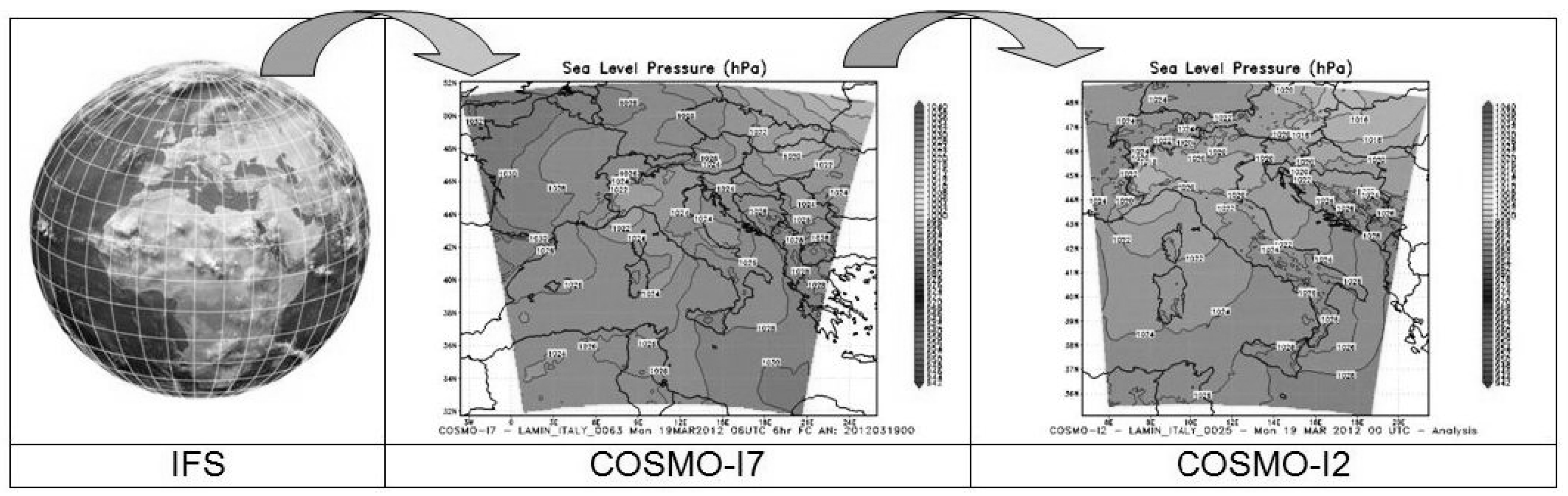
In particular, global NWP models, such as the Integrated Forecasting System (IFS), which is a hydrostatic, two-time-level, semi-implicit, semi-Lagrangian model [9], allow one to describe the weather dynamics with spatial resolution of 10 km, until 2 weeks ahead. Larger time forecasting horizons can be obtained by Limited Area Models, LAM, such as Consortium for Small Scale Modelling (COSMO) I7 and I2, which compute weather forecasts until 72 h ahead [10]. In particular, COSMO-I7 uses as boundary conditions the solutions computed by IFS, and COSMO-I2 is solved in cascade to I7 in order to refine its solution. Hence, the local weather predictions for a certain time horizon are obtained by a physical downscaling, which refines the predictions of two NWP models, as schematically depicted in Figure 1.

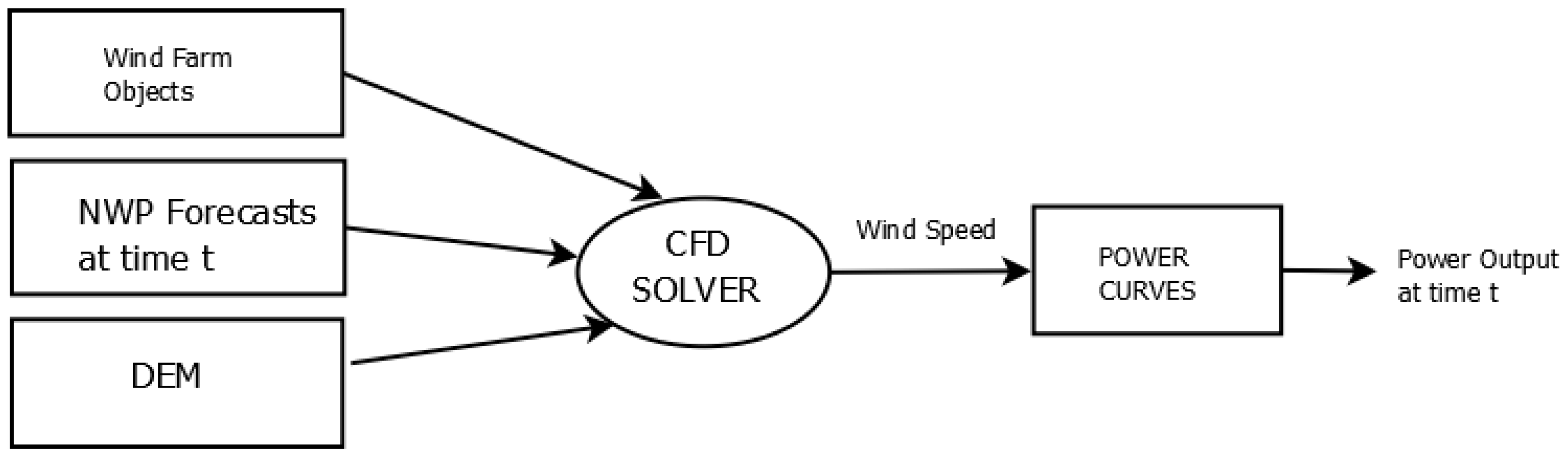
According to this processing paradigm, the solution computed by COSMO-I2 can be further downscaled by a Computational Fluid Dynamics (CFD) solver in order to obtain a more accurate description of the weather variables, and in particular the wind profiles, on a limited geographic area. This principle is currently employed in modern wind power forecasting tools, which try to improve the accuracy of the wind predictions computed by a LAM by solving a detailed physical model of the analyzed area, assuming as boundary conditions the solution computed by the mesoscale model, as schematically depicted in Figure 2. Experimental studies confirmed that the adoption of these physical downscaling-based approaches allows to obtain a sensible improvement of the wind power forecasting accuracy especially for short- and medium-term horizons (30 min to 24 h ahead). This positive feature is mainly due to adoption of high-resolution Digital Terrain Modules-DEM, which allows to accurately describing the orography and roughness of the analysed area, without requiring the need for acquiring and processing anemometric data.

In any case, the main limitations characterizing these CFD-based approaches derive by the large computational resources needed to solve the physical downscaling problem, which could make the problem intractable, or the computing time so high to make the corresponding forecasting solutions not really useful for power system operation.

3. Wind Power Forecasting by Case Based Reasoning

In this paper the role of CBR as enabling methodology for solving the dichotomy between accuracy and promptness in wind power forecasting is analyzed. The main idea is to formalize the physical downscaling problem schematically depicted in Figure 2, as an input/output mapping correlating the boundary conditions of the downscaling problem for the selected geographic area computed by the LAM, to the corresponding downscaled solution computed by the CFD solver. Hence, if we assume that the wind profiles on the analyzed area change according to definite patterns, it can be argued that similar input patterns (boundary conditions) correspond to similar downscaled physical solutions. According to this paradigm, the solution of the local physical model for the assigned boundary conditions can be approximated by processing the downscaled solutions corresponding to the most similar boundary conditions stored in a data-base.

In particular, let X_B be the input matrix storing n boundary conditions, each of them described by a vector of m components, representing the values of the weather variables on a spatial mesh with large resolution; and let Y_B be the output matrix storing the corresponding n downscaled solutions obtained by the CFD solver, each of them described by a vector of r components, representing the wind speed components in the points of interest, i.e., the wind turbines locations. These input/output matrixes represent the knowledge base of the CBR process, since they allow computing the downscaled solution for a boundary condition described by the query vector x_q according to the following procedure:

• Compute the distance between the query point x_q and each vector of the input matrix X_B:

  $$d_j=\sqrt{{\displaystyle \sum }_{i=1}^m{\left({\mathit{x}}_q\left(i\right)-{\mathit{X}}_B\left(j,i\right)\right)}^2}\forall j\in [1,n]$$

  (1)
• Compute the similarity degree between the query and the stored vectors:

  $$w_j=\frac{\underset{i}{\max }(d_i)}{d_j}\forall j\in [1,n]$$

  (2)
• The downscaled solution ${\widehat{\mathit{y}}}_q$ for the query vector can be approximated by processing the downscaled solutions corresponding to the “most similar input vectors”, here referred as the neighbors, which can be identified ordering the input vectors according to their similarity degrees. To this aim, the following naïve approach can be applied:

  $${\widehat{\mathit{y}}}_q\left(i\right)=\frac{{{\displaystyle \sum }}_{j\in N}{\mathit{Y}}_B\left(j,i\right)\times w_j}{{{\displaystyle \sum }}_{j\in N}{w}_j}\forall i\in [1,r]$$

  (3)

  where N is the set of the neighbors.

Alternatively, the previous problem can be solved by a more sophisticated approach based on the solution of the following regression model:

$${\widehat{\mathit{y}}}_q={\mathit{x}}_q\mathit{\beta }$$

(4)

where $\mathit{\beta }$ is the regression matrix, which is obtained as follows:

$$\mathit{\beta }={\left({\mathit{X}}_N^T\right)}^{-1}{\mathit{X}}_N^T{\mathit{Y}}_N$$

(5)

$${\mathit{X}}_N={\mathit{X}}_B\left(j,i\right)\forall j\in N\forall i\in [1,m]$$

(6)

$${\mathit{Y}}_N={\mathit{Y}}_B\left(j,i\right)\forall j\in N\forall i\in [1,r]$$

(7)

It is worth observing that the approximation accuracy of this CBR-based forecasting paradigm is strictly related to the “completeness” of the knowledge base, which depends by the “granularity” of the information represented by the stored input/output patterns. Hence, in order to progressively enhance the knowledge base, an adaptive process aimed at detecting the degradation of the forecasting performances, or the inadequacy of the stored information in correctly representing the input/output mapping, can be used to trigger the rigorous solution of the downscaling problem, and the adjournment of the knowledge base with the corresponding input/output patterns. The first condition can be assessed by performing the ex-post analysis of the forecasting accuracy, i.e., by checking if the forecasting error lies outside a fixed tolerance bound, while the second condition can be assessed by an ex-ante analysis aimed at detecting if the maximum similarity degree between the query vector and the stored input patterns is outside a fixed tolerance bounds, namely if the query vector is too much different from the stored input vectors.

The mathematical backbone of this CBR process is the assessment of the similarity degree, which represents the most critical issue to address, due to the large dimensions of both X_B and Y_B. In fact, these matrixes are characterized by a large number of both rows and columns, depending on the number of available input/output patterns (e.g., order of several hundreds), and the spatial resolution of the environmental variables profile (e.g., order of several thousands), respectively.

Working with these matrixes is a very demanding task, since also the most elementary operations require large computing and storage resources, making the deployment of conventional mathematical operators not suitable. Another complex issue to address in this domain is the assessment of the vectors similarity, since in high-dimension spaces the conventional distance metrics could degenerate, becoming uniform, and the nearest neighbor notion loses of meaning, due to its poor discrimination feature. In the computational intelligence literature, this phenomenon is referred as the curse of dimensionality problem, which represents one of the most challenging issue to address in the context of Big Data analytics [11]. To solve this issue in this paper the adoption of feature extraction techniques based on PCA, and PLSR is explored.

4. Enabling Methodologies for Feature Extraction from Massive Wind Data

Feature extraction techniques based on PCA and PLSR have been recently proposed in the wind forecasting literature in an attempt to reduce the complexity of identification models. In particular, in [12] PCA is integrated in a statistical wind-forecasting algorithm in order to reduce the cardinality of a time delay-matrix, simplifying the solution of the time regression problem. According to the same principle, in [13] a PCA-based technique is employed to reduce the cardinality of the training set of a neural network aimed at improving the wind forecasting accuracy of a mesoscale model, while in [14] the same technique is employed to select the most suitable inputs for a semi-physical forecasting method. Moreover, in [15] a method based on PLSR is adopted in an ensemble-forecasting framework to determine the weighting factors to assign in combining the output of multiple forecast algorithms.

These papers demonstrate the effectiveness of PCA and PLSR based techniques in extracting the most relevant information codified in large datasets of historical input/output observations. This is obtained by projecting the vectors composing the original dataset in a transformed space, which allows describing the information codified in the dataset with a reduced number of vector components. This cardinality reduction feature could play an important role in solving the curse of dimensionality problem in wind forecasting, which is one of the main contributions of this paper. Hence, after presenting the mathematical fundamentals of these two techniques, their integration in a CBR-based wind-forecasting framework is discussed.

4.1. PCA: Principal Component Analysis

The goal of PCA is to deflate the dimension of a dataset guaranteeing the lowest information losses, by projecting the vector composing the original dataset by a proper orthogonal base aimed at maximizing the data variance.

The application of PCA to the problem under study asks for decomposing the input/output matrixes as follows:

$${\mathit{X}}_B={\overline{\mathit{X}}}_B+{\mathit{X}}_{Bs}{\mathit{P}}^T+{\mathit{ϵ}}_x$$

(8)

$${\mathit{Y}}_B={\overline{\mathit{Y}}}_B+{\mathit{Y}}_{Bs}{\mathit{Q}}^T+{\mathit{ϵ}}_y$$

(9)

where:

• ${\overline{\mathit{X}}}_B$ and ${\overline{\mathit{Y}}}_B$ are the center of the matrixes ${\mathit{X}}_B$ and ${\mathit{Y}}_B$, respectively;
• ${\mathit{X}}_{Bs}$ and ${\mathit{Y}}_{Bs}$, whose dimensions are $[n_{PCx},n]$ and $[n_{PCy},n]$ ${(\mathrm{with}n}_{PCx}\ll {m,n}_{PCy}\ll r$), are the score matrixes;
• $\mathit{P}$ and $\mathit{Q}$, whose dimensions are $[n{,n}_{PCx}]$ and $[n{,n}_{PCy}]$, respectively, are the loadings matrixes;
• ${\mathit{ϵ}}_x$ and ${\mathit{ϵ}}_y$ are the error matrixes.

The components of the loading matrixes $\mathit{P}$ and $\mathit{Q}$ can be computed by using an iterative approach that maximizes the variables variance, constraining the column vectors of these matrixes to be the eigenvectors of the covariance matrixes:

$$\begin{gathered} \mathit{\Sigma }\propto {\left({\mathit{X}}_B{\mathit{w}}_k\right)}^T={\left({\mathit{X}}_B{\mathit{w}}_p\right)}^T={(\mathit{w}}_k^T{\mathit{X}}_B^T{\mathit{X}}_B{\mathit{w}}_p)={\mathit{w}}_k^T{\lambda }_p{\mathit{w}}_p={\lambda }_p{\mathit{w}}_k^T{\mathit{w}}_p \\ k,p\in [1,m] \end{gathered}$$

(10)

where, $\mathit{\Sigma }$ represents the linear correlation between two random variables.

Hence, the corresponding elements of the scoring matrixes can be computed as:

$${\widehat{\mathit{X}}}_{bf}={\mathit{X}}_B-{\displaystyle \sum }_{\mathit{s}=1}^{f-1}{\mathit{X}}_B{\mathit{p}}_s{\mathit{p}}_s^T$$

(11)

$${\widehat{\mathit{Y}}}_{bf}={\mathit{Y}}_B-{\displaystyle \sum }_{\mathit{s}=1}^{f-1}{\mathit{Y}}_B{\mathit{q}}_s{\mathit{q}}_s^T$$

(12)

where ${\mathit{p}}_s$ and ${\mathit{q}}_s$ are the s-th column vectors of the loadings matrices P and Q, respectively, and f is the number of principal components, which can be selected by applying the methodologies described in [16].

4.2. Partial Last Square Regression

PLSR aims at extracting an orthogonal set from a set of “latent variables”, which contains the most relevant information codified in the original dataset [17]. This can be obtained by representing the knowledge based according to the following equations:

$$\{\begin{array}{c}{\mathit{X}}_B={\overline{\mathit{X}}}_B+{\mathit{X}}_{Bs}{\mathit{P}}^T+{\mathit{\epsilon }}_x\\ {\mathit{Y}}_B={\overline{\mathit{Y}}}_B+{\mathit{Y}}_{Bs}{\mathit{Q}}^T+{\mathit{\epsilon }}_y\end{array}$$

(13)

Similarly to PCA, at each iteration PLSR tries to maximize the covariance between ${\mathit{X}}_B$ and ${\mathit{Y}}_B$, by projecting these data in a new space [16], but, in addition, it includes a regression step, which allows to compute two further variables, namely the regression matrix $\mathit{\beta }$, and the intercept ${\mathit{\beta }}_0$. These variables allow to approximate the output matrix Y_B as follows:

$${\widehat{\mathit{Y}}}_B={\mathit{\beta }}_0+{\mathit{X}}_B\mathit{\beta }$$

(14)

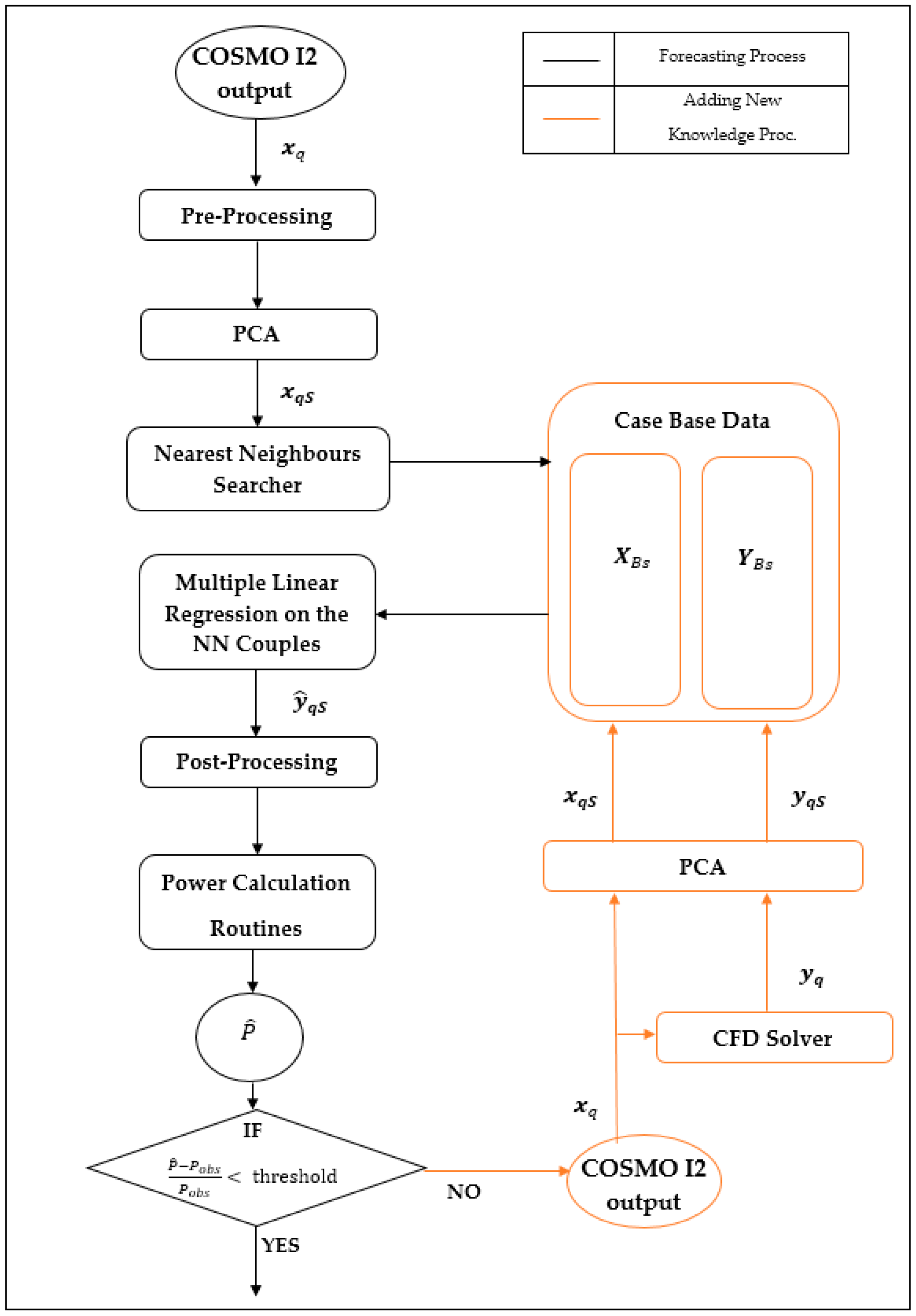
4.3. Proposed Method

To deal with the curse of dimensionality problem in CBR-based wind power forecasting, the application of PCA and PLSR-based techniques is proposed in this paper. The idea is to extract actionable intelligence from the knowledge base of the CBR process, by projecting the input/output vectors in a transformed domain, which is characterized by lower dimensionalities. In this domain the vectors can be represented by a limited number of components, and both the similarity assessment and the regression analysis can be performed more effectively.

The first step in deploying the proposed framework is to build the knowledge base of the CBR module by solving the physical downscaling problem for a comprehensive set of boundary conditions generated by the mesoscale model. To this aim a CFD model aimed at computing the wind and pressure field on a high-resolution spatial grid is employed. The CFD allows to accurately representing the area under study by a high-resolution Digital Elevation Model (DEM), which integrates detailed information on the orography and roughness of the terrain. The solutions computed by the CFD are organized in the matrixes X_B and Y_B, which are processed by a feature extraction technique based on PCA or PLSR. The corresponding reduced matrixes, X_Bs and Y_Bs, are stored in the database of the historical physical downscaling solutions, and used to infer the solutions for the query vectors. The overall forecasting process is summarized in Figure 3.

5. Experimental Results

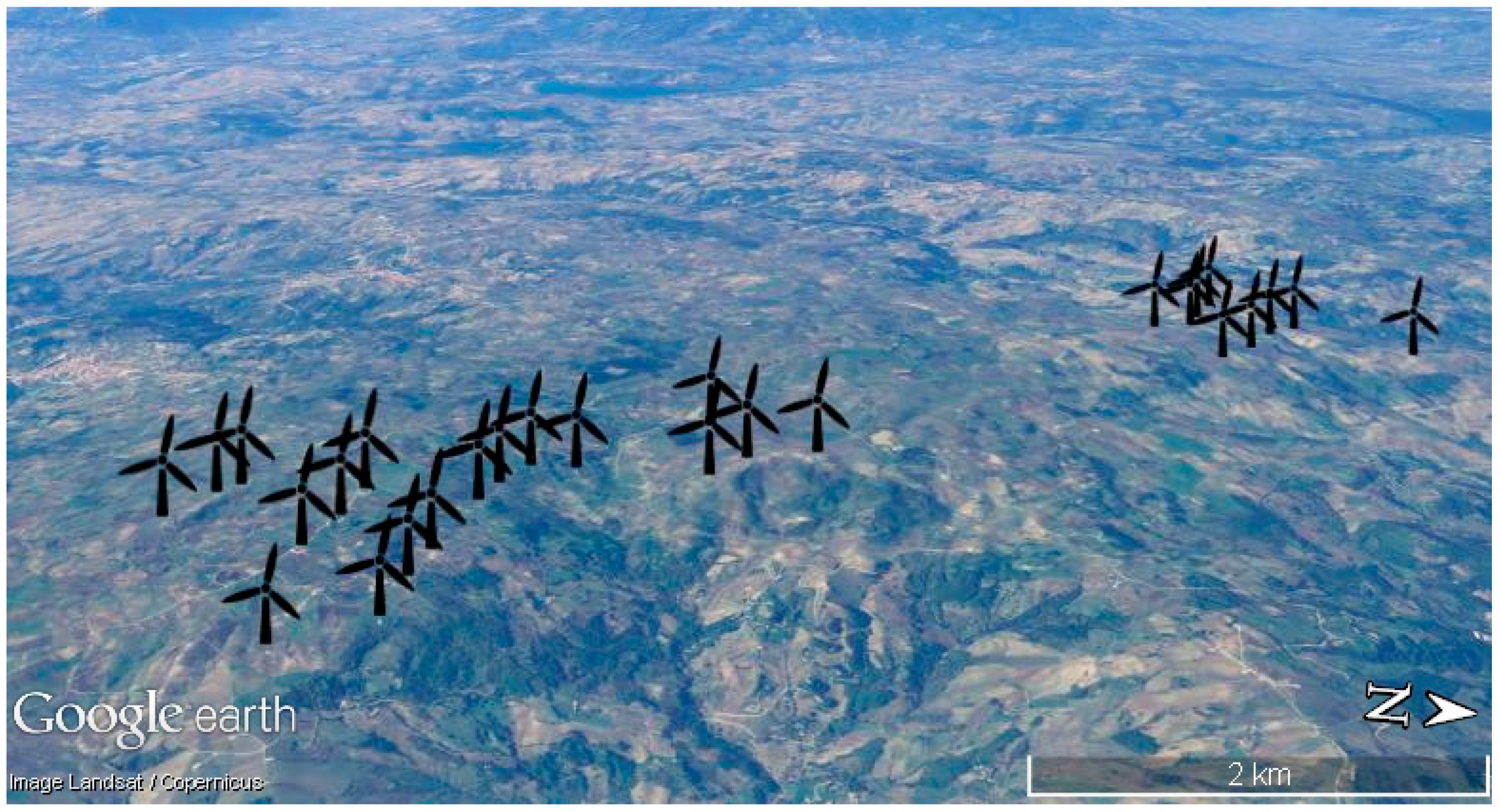
To assess the benefits deriving by the application of the proposed framework in the task of solving complex forecasting problems, detailed experimental results are here described. The analyzed area, which is schematically indicated in Figure 4, is located in the south of Italy, in a region characterized by a massive pervasion of wind generators. The morphology of this area is very complex, the ridges are steep, the territory is mainly rural with agricultural and wooded areas. The installed wind power capacity for the entire area is 70.2 MW, which is shared among 27 machines directly connected to the power transmission system by a HV power line. This line is frequently congested due to the large wind power production, and in many operation conditions it represents the bottleneck for the entire power system capability, inducing sensible differences of the local marginal prices. To assess the benefits deriving by the application of the proposed framework in predicting power congestions and defining effective mitigation strategies for this area, ten days characterized by critical contingencies have been selected and analyzed in this study.

The forecast profiles for each hour of the next day are computed by the mesoscale model for the area under study have been furnished by Italian Aerospace Research Center (CIRA). These data are organized on a spatial grid composed by 16 × 18 points (spatial resolution of 2.8 km), for 62 layers, ranging from about 4 m to 20 km on the terrain ground. The DEM for the area under study has been developed by the CNR-IREA (Institute for Electromagnetic Measurements of the Environment). The employed CFD solver solves mathematically the Reynolds Average Navier Stokes equation (RANS) using finite volume method and is based on Phoenix software package, which adopts traditional CFD techniques to model the atmospheric dynamics.

5.1. PCA Results

A preliminary sensitivity analysis is performed to identify the optimal PCA algorithm set points. After this analysis the CBR-based framework has been adopted to solve the forecasting problem for 16 cases, requiring a solution time of the order of 4 min, against the 2 h required for solving the corresponding case by the CFD solver. The results obtained are summarized in

Table 1. Performance Indexes: Proposed Method.

Case Number	N° xPCs (${\mathit{k}}_{{\mathit{X}}_{\mathit{B}}}$)	N° yPCs (${\mathit{k}}_{{\mathit{Y}}_{\mathit{B}}}$)	Nearest Neighbors (NN)	Normal Root Mean Square Error (NRMSE)	Normal BIAS (NBIAS)	Normal Mean Absolute Error (NMAE)
1	5	5	3	0.5204	0.2063	0.4439
2	10	12	3	0.3995	0.0166	0.3403
3	5	5	6	0.4195	0.2599	0.3629
4	5	5	3	0.2994	−0.0412	0.2366
5	10	12	3	0.3039	0.0864	0.2594

, and demonstrate the good accuracy of the proposed method, although a reduced number of historical information is stored in the knowledge base. More detailed results are shown in Figure 5, Figure 6, Figure 7 and Figure 8.

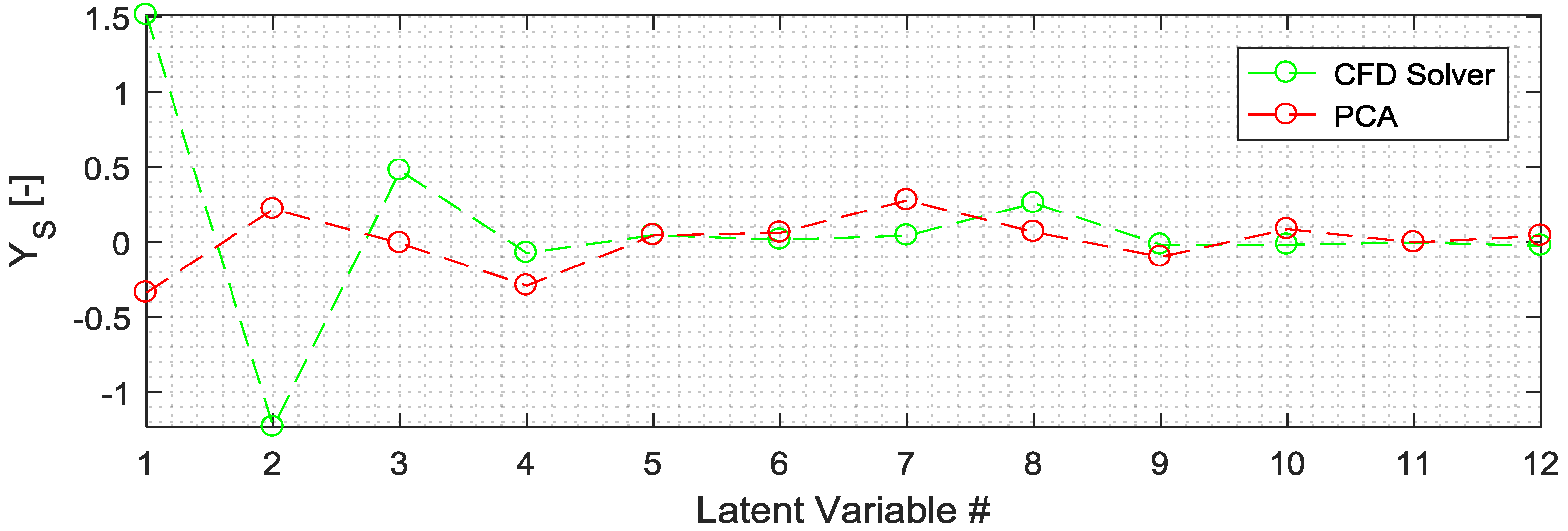
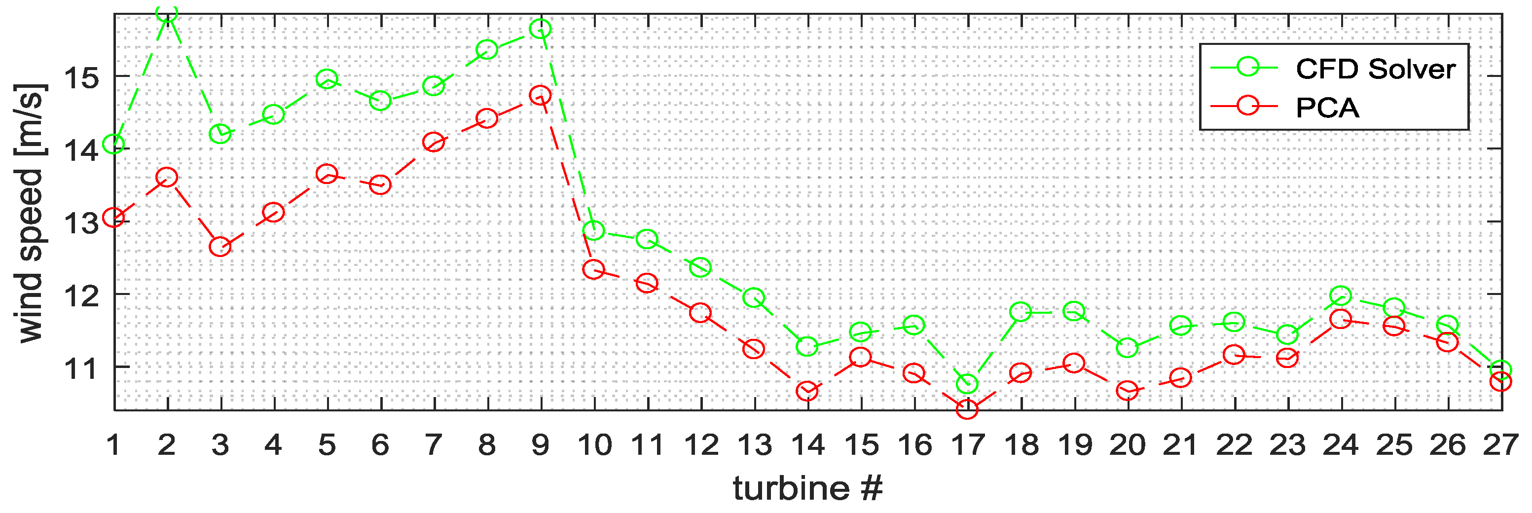
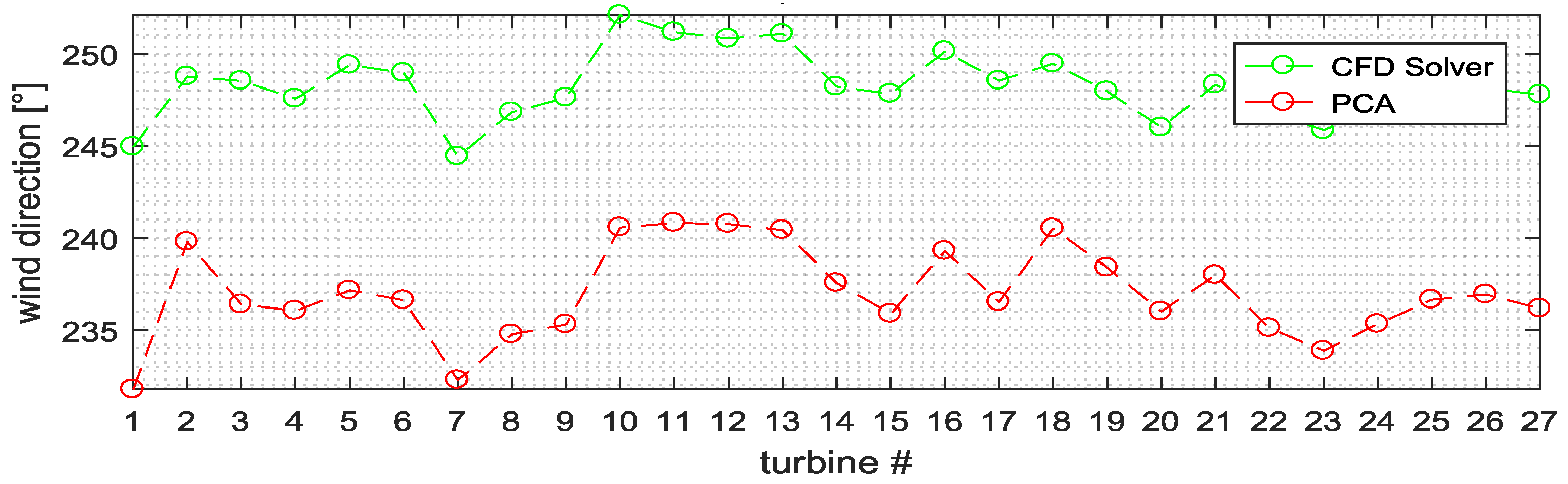
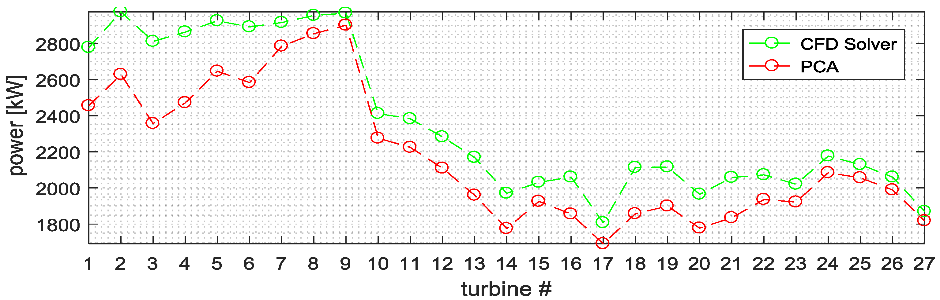
Figure 5 shows the comparison between the Principal Components (PC) estimated (red) and obtained applying PCA to the CFD outputs in the validation period (green). In Figure 6, Figure 7 and Figure 8 the wind speed, the wind direction, and the generated power for each turbine of the windfarm estimated by using the proposed method (red) and the CFD (green) are reported.

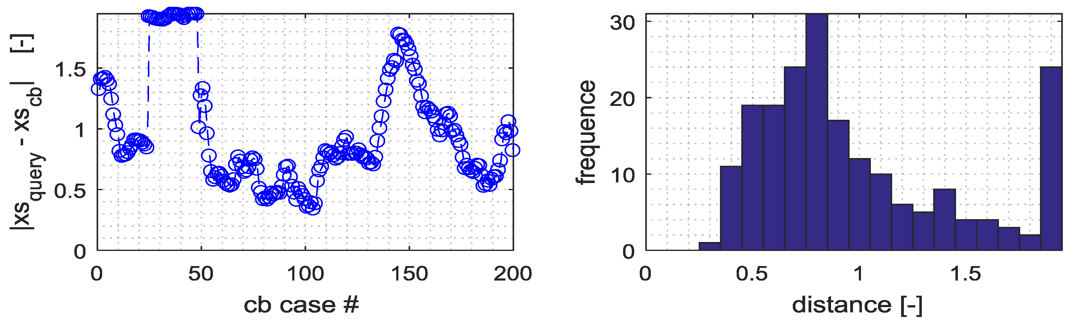
These figures confirm the good degree of accuracy obtained by the proposed method, although the estimation of the first latent variables needs to be improved, since higher forecasting errors are observed. This is also confirmed in Figure 9, which reports, for a fixed forecasting hour, the distances of Nearest Neighbors case by the query vector, and the probabilistic distribution of these distances.

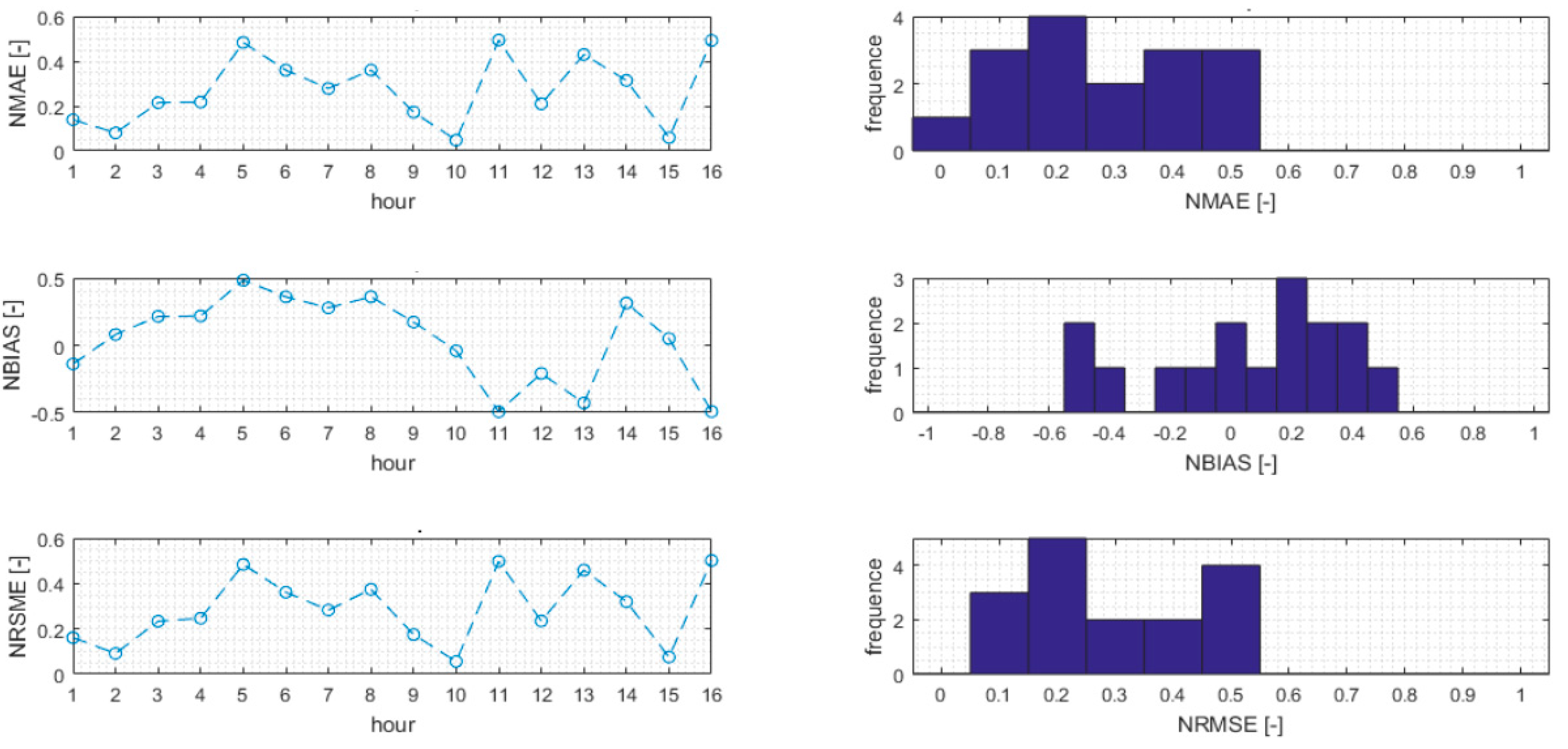
Moreover, Figure 10 reports some interesting figure of merits characterizing the accuracy of the proposed method, which include the NMAE trend on each hour unit of time of validation period, the related distribution of the NMAE values, the NBIAS trend on each hour unit of time of validation period, the related distribution of NBIAS values, the NRSME trend on each hourly unit of time of validation period, and the related distribution of NRSME values.

These results confirmed the need for increasing the number of historical cases in order to reduce the distance between the query point and the neighbors, which is the main factor affecting the overall forecasting accuracy.

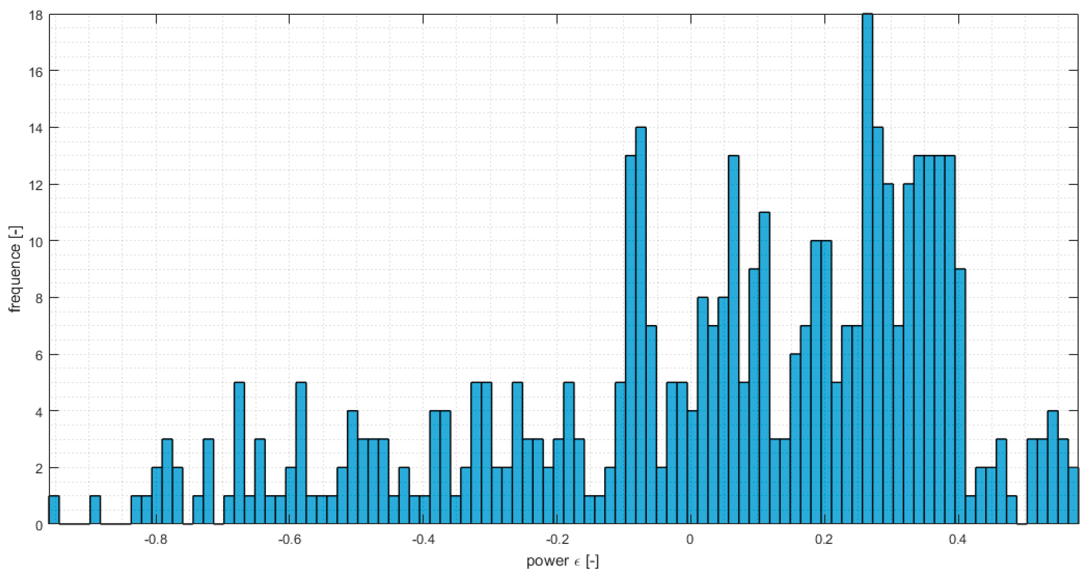
Finally, in Figure 11 the probabilistic distribution of the error between the power output estimated by the proposed method, and by the CFD solver for the validation period is reported. The results show a slight underestimation of the estimated power, which in most cases is of the order 10%.

5.2. PLSR Results

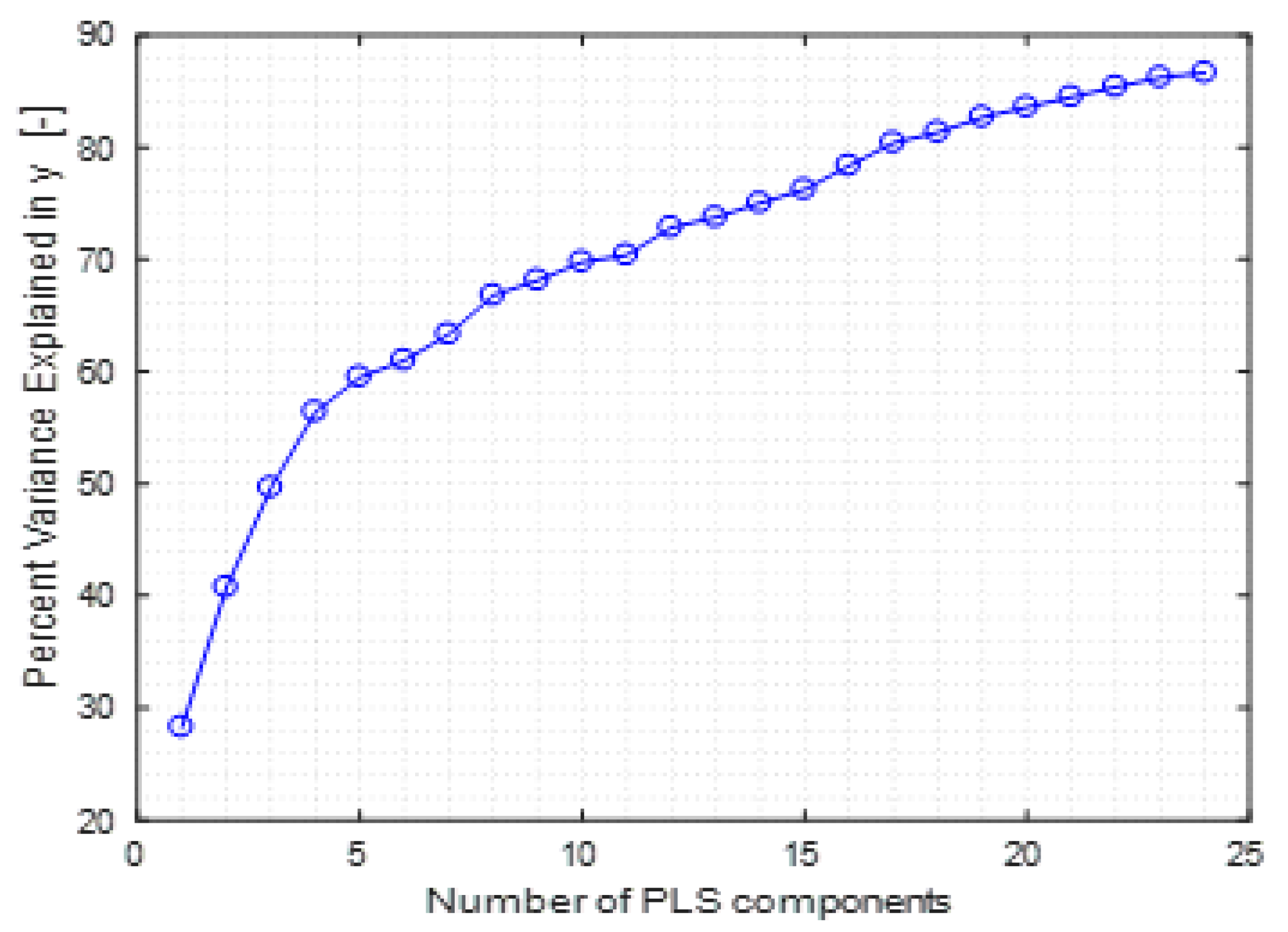
The first experiments developed have been based on the application of PLSR for reducing the cardinality of the matrixes ${\mathit{X}}_B$ and ${\mathit{Y}}_B$. To this aim, the choice of the proper number of PCs has been done by analyzing the evolution of the variance in ${\mathit{Y}}_B$ versus the number of PCs, which is reported in Figure 12. The optimal number of principal components is given by the analysis on the cumulative variance expressed by the PC. In this chase, the first 24 principal components explain over 90% of the cumulative variance. Obviously, a larger number of components is expected to improve the approximation accuracy and the computational burden, as it can be observed by analyzing the data summarized in

Table 2. Performance Indexes using PLSR.

Case	RMSE on Wind Speed (m/s)	RMSE on Wind Direction (°)	Time Required	N° of PCs	Rsquared Ratio
1	1.7865	25.5	6.10 s	24	0.8355
2	2.1861	27.8	2.87 s	12	0.7581
3	1.6119	24.0	11.39 s	48	0.8538

.

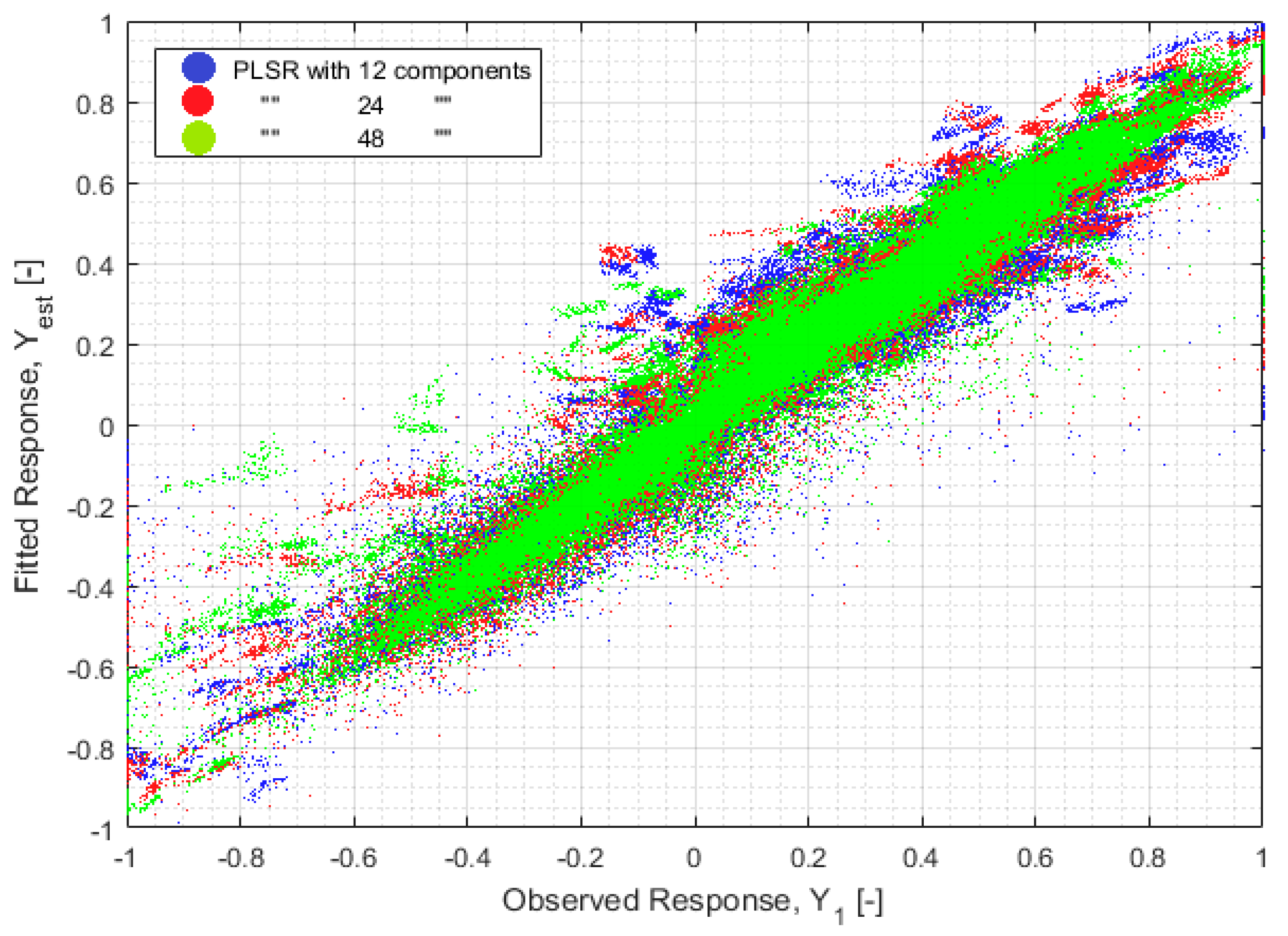
As expected, the case characterized by the largest number of components, namely case 3, is the one characterized by the better approximation accuracy on both wind speed and direction, and the largest computational burden. This is also confirmed in Figure 13, which depicts the scatter plot of the original versus the reconstruction variables. This graph highlights the important role played by the selection of the optimal number of components in improving the approximation performances of PLSR-based methods. In particular, it could be note that increasing the PC number, increases the accumulation of the points nearby the first quadrant bisector, hence leading to a better approximation accuracy.

Finally, it should be noted that the limited number of available observations in the knowledge base does not allow the PLSR-based CBR module to extract enough information, leading to unsatisfactory forecasting accuracy. In these conditions the PCA-based technique represents the most viable solution for CBR-based forecasting. A different trend is expected for larger observations. The experimental validation of this issue is currently under development by the authors.

6. Conclusions

This paper has proposed a novel method for time and spatial wind power forecasting, which is based on a process of knowledge discovery from big data. The main idea is to integrate Partial Least Squares Regression, and Principal Component Analysis in a Case-based Reasoning module, in order to effectively process massive data sets, addressing the curse of dimensionality problem. The obtained results obtained on a real case study have shown the effectiveness of the proposed method in the task of obtaining approximate and fast forecasting problem solutions, by avoiding unnecessary physical model solutions for similar boundary conditions. This has been obtained by extracting the most relevant information codified in the boundary conditions by projecting the corresponding descriptive vectors in new space domains characterized by a reduced number of dimensions. This important feature allowed us to infer the forecasting solution corresponding to new boundary conditions by processing the historical physical model solutions corresponding to the most similar boundary conditions, and to detect when the knowledge base need to be adjourned in order to improve the granularity of the stored information. The authors are confident that the conceptualization of feature extraction techniques based on the proposed CBR paradigm could support the analyst in identifying the most valuable variables influencing the input/output forecasting mapping, which might help the design of the link between future models showing where detail may be more and less important. This issue is currently under development by the Authors.