Circulating Current Reduction Strategy for Parallel-Connected Inverters Based IPT Systems

Abstract

Multiple inverters connected in parallel is a promising method to upgrade the power capacity of inductive power transfer (IPT) systems. Due to a slight unbalance of the control signals, the inner resistances of the inverters and other uncertainties, circulating currents exist among the parallel units which reduce the reliability of IPT systems. Firstly, the series-parallel resonant tank is employed in the multiple inverters based IPT system to eliminate the DC and harmonic circulating currents. The fundamental circulating currents in the paralleled inverter units are analyzed in detail. Then, for eliminating the fundamental circulating currents, a current decomposition method and a control diagram are proposed to avoid acquiring the phase of the current by detecting zero cross current point which increases the accuracy of the control algorithm. Finally, a 1-kW parallel-connected inverter IPT system is provided to verify the proposed approach. The experimental results show that the proposed method is effective for eliminating the fundamental circulating currents. The maximum efficiency of the system is up to 92.18% which is 0.53% higher compared to that without the current phasor control (91.65%).

1. Introduction

Conventional inductive power transfer (IPT) systems, consisting of a DC power supply, a single high frequency inverter, a resonant compensation unit, loosely coupled coils and a secondary energy management unit, have been widely used in industrial high power applications [1,2,3,4] and charging systems for public electric vehicles [5,6,7,8,9]. The high frequency inverter converts the input DC voltage into a high frequency AC voltage for the primary coil. The high frequency AC energy can be transferred through loosely coupled coils. Then, the rectifier of the secondary side converts the received high frequency AC voltage into a DC voltage for the load. However, the single inverter feeding based IPT system mentioned above is normally designed to meet the demand of a fixed output power rating. The capability of the IPT system is sometimes decided by the capacity of the inverter. It should be noted that it is not easy to achieve high power transfer with a single inverter in the IPT system, due to the capacity and cost restriction of power switches [10,11]. Except the IPT system, the power extension is restricted by the switches in the other applications of the converters. The parallel connected method is a well-adapted solution, and used in many field, e.g., photovoltaic (PV) plants, DC-DC converters, inductive heating and so on [12,13,14]. However, there are few reports on the application of this parallel connected method in the field of IPT.

In order to meet the requirements of high-power applications, e.g., the power supplying for high-speed trains, the charging system for public vehicles [15,16,17], quite a few methods have been proposed to increase the capacity of IPT systems in the past decade. They can be roughly classified into three categories: the cascaded method, the parallel connected method and the magnetic field enhancement method. For the cascaded method, an effective power improvement method based on the cascaded multi-level inverter technology has been discussed in [18]. The phase shift pulse width modulation method employed in the cascaded multi-level inverter to realize the power regulation and the selective harmonic elimination, simultaneously. Nevertheless, the modulation method of the control signal is some kind of complexities and the dynamic performance was not discussed. For the magnetic field enhancement method, a novel IPT topology based on dual coupled transmitters is proposed in [19,20]. By configuring the additional compensation capacitors, resonant inverters with different power ratings can be connected in parallel to achieve the high power transfer. However, it is difficult to choose the additional capacitors to let the inverter work under resonant condition and achieve power sharing due to the inevitable component tolerances. For the parallel connected method, a straightforward method of improving the power levels is that employing the parallel-connected inverter topology for feeding IPT systems [10,21]. A power regulation and selective harmonic current elimination approach of parallel-connected inverter is proposed in [21] for supplying IPT systems, which not only can upgrade the capacity of the power supply, but also can suppress the total harmonic distortion (THD) of the primary coil current. Unfortunately, the inevitable circulating current issue caused by the component tolerance has not been discussed in detail.

Circulating currents can not only damage the power electronic devices and lower the efficiency of the system by introducing some unnecessary currents. In addition, they can even reduce the reliability of the system by imposing too much current stress on the semiconductor devices. The circulating current usually consists of DC circulating component, harmonic circulating component and fundamental circulating component. An unneglectable DC circulating current between the inverters caused by a slight unbalance of the control signals, the inner resistances of the inverters and the speed difference of the switching drivers [22]. The harmonic circulating current [23] should be considered in the parallel-connected inverter IPT system, due to the high THD of the inverter output voltage [10] and the tolerance of circuit parameters when the inverter adopts the phase shift control technology. Besides, the fundamental circulating current exists between the parallel inverter units [21] due to the unbalance of parallel connected inverters, such as the gate pulse delay, the pulse width modulator randomness and the control delay. As a result, the electric and thermal stresses are unbalanced between the parallel inverters [24,25], and it will increase the potential damage to the IPT system. Hence, it is necessary to investigate an approach to reduce the circulating current in the parallel-connected inverter IPT system.

It is an effective approach for eliminating the DC and harmonic circulating currents between the parallel units by adding the series-parallel resonant tank proposed in [11] rather than with complex control methods [22,23]. For the fundamental circulating currents, a phasor control method is proposed in [11] with the function of eliminating the fundamental circulating currents. Nevertheless, the proposed circulating current elimination method needs phase locking loop (PLL) circuits to track the phase of the bus voltage to calculate the active and reactive current components [11,26], which increases the computational burden and complexity of the control algorithm. Moreover, it is not easy to obtain the phase of the current accurately due to relatively high fundamental frequency. Usually, comparators are needed to acquire the phase of the current by detecting zero cross current point [27]. However, in practice, the current signal is not always reliable due to the distortion. As a consequence, the false synchronization pulse generated by the comparators can lead to the incorrect calculation of the current phase [28]. The fundamental circulating current problem is deliberately overcome by an active and reactive power decomposition method proposed in [17] without PLL. However, both the DC and harmonic circulating currents are not analyzed or minimized in [17]. An extra LC filter is needed to be added in the compensative circuit.

In order to overcome the aforementioned drawbacks, this paper applies a novel series-parallel tuned parallel-connected inverter IPT system to eliminate the DC and harmonic circulating currents without any control strategy which is proposed in [23]. In addition, the circulating current eliminating strategy is analyzed in detail in Section 2. In order to eliminate the fundamental circulating current, this paper focuses on developing an active and reactive current decomposing approach without PLL and a phasor control method. With the current decomposing method, the high frequency AC signals can be transformed to DC signals for the phasor controllers, which decreases the computational burden and complexity of the control algorithm. It provides convenience for the power extension through the coordination between the multiple resonant inverter units and the current decomposing circuits which reduces the manufacturing cost.

This paper is organized as follows. Section 2 presents the principle description of the parallel-connected inverter topology. Section 3 analyses the causes of the fundamental circulating currents in the inverter units. A current decomposition method and a control diagram are proposed in Section 4. The experimental results from a 1-kW parallel-connected inverter IPT system are provided in Section 5 to verify the validity of the circulating current reducing and constant voltage control approaches. Finally, this paper is concluded in Section 6.

2. Principle Description of the Parallel-Connected Inverter Topology

The schematic of the IPT system based on the parallel-connected inverter with the series-parallel resonant tank is shown in Figure 1, which consists of n identical inverter units with the same operating frequency $\omega$. For tuning purposes, the series-parallel resonant tank ($L_{\mathrm{a}k}$, $C_{\mathrm{a}k}$, $L_{\mathrm{b}k}$ and $C_{\mathrm{b}k}$) for the kth parallel unit should satisfy:

$$\omega =\frac{1}{\sqrt{L_{\mathrm{a}k}{C}_{\mathrm{a}k}}}=\frac{1}{\sqrt{L_{\mathrm{b}k}{C}_{\mathrm{b}k}}}(k=1,2,3\cdots n)$$

(1)

The kth parallel unit is connected in series with a connection inductor $L_{\mathrm{e}k}$, which is used to suppress the circulating current in the parallel-connected inverter IPT system. The value of $L_{\mathrm{e}k}$ is very small, so that the voltage drop and power losses over the resistance of connection inductors can be neglected [29]. The compensation capacitor $C_{\mathrm{P}}$ is connected in series with the primary coil $L_{\mathrm{P}}$. The secondary circuit is consisted of the secondary coil $L_{\mathrm{S}}$, the compensation capacitor $C_{\mathrm{S}}$, the rectifier and the load $R_{\mathrm{L}}$. For tuning purposes, $L_{\mathrm{P}}$, $C_{\mathrm{P}}$, $L_{\mathrm{S}}$ and $C_{\mathrm{S}}$ are all designed at the resonant frequency:

$$\omega =\frac{1}{\sqrt{L_{\mathrm{P}}{C}_{\mathrm{P}}}}=\frac{1}{\sqrt{L_{\mathrm{S}}{C}_{\mathrm{S}}}}$$

(2)

Without loss of generality, we take the parallel three-inverter based IPT system as an example, and three cases will be discussed in this section. According to [30], the reflected resistance of the secondary circuit is given as:

$$R_{\mathrm{r}}=\frac{{\omega }^2{\pi }^2{M}^2}{8R_{\mathrm{L}}}$$

(3)

Firstly, the parallel three-inverter IPT system without the series-parallel resonant tank has been discussed in [21] and the equivalent circuit is shown in Figure 2.

By employing the phase-shift control technology in the parallel-connected inverter IPT system [10], the output voltage waveforms are shown in Figure 3. The fundamental magnitude of the inverter output voltage (u₁(1), u₂(1) and u₃(1)) can be regulated by changing the conduction angle ${\theta }_{\mathrm{L}}$ varied from 0° to 180° as shown in Equation (4):

$$\{\begin{array}{l}{u}_1=\frac{E_{1\mathrm{H}}-E_{1\mathrm{L}}}{2}+{\displaystyle \sum _{k=1}^{\infty }[\frac{2(E_{1\mathrm{H}}+E_{1\mathrm{L}})}{k\pi }\cos (\frac{k{\theta }_{\mathrm{L}1}}{2})\sin (k\omega t)]}\\ u_2=\frac{E_{2\mathrm{H}}-E_{2\mathrm{L}}}{2}+{\displaystyle \sum _{k=1}^{\infty }[\frac{2(E_{2\mathrm{H}}+E_{2\mathrm{L}})}{k\pi }\cos (\frac{k{\theta }_{\mathrm{L}2}}{2})\sin (k\omega t+k{\theta }_{\Delta 12})]}\\ u_3=\frac{E_{3\mathrm{H}}-E_{3\mathrm{L}}}{2}+{\displaystyle \sum _{k=1}^{\infty }[\frac{2(E_{3\mathrm{H}}+E_{3\mathrm{L}})}{k\pi }\cos (\frac{k{\theta }_{\mathrm{L}3}}{2})\sin (k\omega t+k{\theta }_{\Delta 13})]}\end{array}k=1,3,5,7...$$

(4)

At the same time, the phase angle ${\theta }_{\Delta }$ among the inverter 1, inverter 2 and inverter 3 can be altered accordingly. Due to the inner resistances of the inverters [22], the positive level of the inverter output voltage is not equal to the negative one ($E_{1\mathrm{H}}\ne E_{1\mathrm{L}}$, $E_{2\mathrm{H}}\ne E_{2\mathrm{L}}$ and $E_{3\mathrm{H}}\ne E_{3\mathrm{L}}$). Meanwhile, the conduction angle of the positive voltage level is not equal to the negative one (${\theta }_{\mathrm{L}1}\ne {{\theta }_{\mathrm{L}1}}^{\prime }$, ${\theta }_{\mathrm{L}2}\ne {{\theta }_{\mathrm{L}2}}^{\prime }$ and ${\theta }_{\mathrm{L}3}\ne {{\theta }_{\mathrm{L}3}}^{\prime }$) due to a slight unbalance of the control signal and the speed of the switching drivers. Hence, there is a DC voltage offset in the inverter output voltage as shown in Figure 3. Meanwhile, by employing the phase shift control technology, the THD of the parallel inverter output voltage is high [10]. Therefore, the difference of the DC voltage offset $\Delta u_{\mathrm{DC}}$, the difference of the fundamental voltage $\Delta u_{\mathrm{Fun}}$, and the difference of the harmonic voltage $\Delta u_{\mathrm{Har}}$ can be derived by:

$$\{\begin{array}{l}\Delta u_{\mathrm{DC}}=\frac{E_{1\mathrm{H}}-E_{1\mathrm{L}}}{2}-\frac{E_{2\mathrm{H}}-E_{2\mathrm{L}}}{2}-\frac{E_{3\mathrm{H}}-E_{3\mathrm{L}}}{2}=\frac{E_{1\mathrm{H}}+E_{2\mathrm{H}}+E_{3\mathrm{H}}-E_{1\mathrm{L}}-E_{2\mathrm{L}}-E_{3\mathrm{L}}}{2}\\ \Delta u_{\mathrm{Fun}}=\frac{2(E_{1\mathrm{H}}+E_{1\mathrm{L}})}{\pi }\cos (\frac{{\theta }_{\mathrm{L}1}}{2})\sin (\omega t)-\frac{2(E_{2\mathrm{H}}+E_{2\mathrm{L}})}{\pi }\cos (\frac{{\theta }_{\mathrm{L}2}}{2})\sin (\omega t+{\theta }_{\Delta 12})\\ -\frac{2(E_{3\mathrm{H}}+E_{3\mathrm{L}})}{\pi }\cos (\frac{{\theta }_{\mathrm{L}3}}{2})\sin (\omega t+{\theta }_{\Delta 13})\\ \Delta u_{\mathrm{Har}}={\displaystyle \sum _{k=3}^{\infty }\begin{array}{l}[\frac{2(E_{1\mathrm{H}}+E_{1\mathrm{L}})}{k\pi }\cos (\frac{k{\theta }_{\mathrm{L}1}}{2})\sin (k\omega t)-\frac{2(E_{2\mathrm{H}}+E_{2\mathrm{L}})}{k\pi }\cos (\frac{k{\theta }_{\mathrm{L}2}}{2})\sin (k\omega t+k{\theta }_{\Delta 12})]\\ -\frac{2(E_{3\mathrm{H}}+E_{3\mathrm{L}})}{k\pi }\cos (\frac{k{\theta }_{\mathrm{L}3}}{2})\sin (k\omega t+k{\theta }_{\Delta 13})]\end{array}}\end{array}k=3,5,7...$$

(5)

Compared to the inductive reactance ($L_{\mathrm{e}1}$, $L_{\mathrm{e}2}$ and $L_{\mathrm{e}3}$), the resistance of the connection inductors ($R_{\mathrm{Le}1}$, $R_{\mathrm{Le}2}$ and $R_{\mathrm{Le}3}$) is much smaller, so that it can be neglected. Therefore, with a slight DC voltage offset difference there will be a huge DC circulating current between the parallel units [22]. Due to the tolerance of circuit parameters and the voltage difference mentioned in Equation (5), the fundamental circulating currents $\Delta i_{\mathrm{Fun}1}$ and $\Delta i_{\mathrm{Fun}2}$, the harmonic circulating currents $\Delta i_{\mathrm{Har}1}$ and $\Delta i_{\mathrm{Har}2}$ between the parallel units also exist [23]. Three kinds of the circulating currents mentioned above, can be eliminated effectively by increasing the impedance of connection inductors ($L_{\mathrm{e}1}$, $L_{\mathrm{e}2}$ and $L_{\mathrm{e}3}$). Nevertheless, the connection inductors will be heavy and bulky, increasing the costs and volume, and soften the characteristic of the output voltage of the inverter [31,32].

Secondly, for the sake of eliminating the DC circulating currents $\Delta i_{\mathrm{DC}1}$ and $\Delta i_{\mathrm{DC}2}$, a series resonant tank ($L_{\mathrm{a}k}$ and $C_{\mathrm{a}k}$) is connected to each parallel unit branch in series, which can isolate the DC current effectively shown in Figure 4. For eliminating the harmonic circulating currents $\Delta i_{\mathrm{Har}1}$ and $\Delta i_{\mathrm{Har}2}$, the quality factor of the series resonant tank, defined as the ratio of the impedance of the series resonant inductor to the equivalent resistor of the load [29], should be large enough. Nevertheless, the larger the quality factor of the series resonant tank is, the heavier the inductor will be. When the inductance of the series resonant tank is huge, it will be difficult to find a space to host it. Therefore, it is not a good choice to increase the quality factor of the series resonant tank to eliminate the harmonic circulating currents $\Delta i_{\mathrm{Har}1}$ and $\Delta i_{\mathrm{Har}2}$ for the parallel-connected inverter IPT system.

Thirdly, in order to eliminate the harmonic circulating currents $\Delta i_{\mathrm{Har}1}$ and $\Delta i_{\mathrm{Har}2}$, a parallel resonant tank which can filter out the harmonic other than the fundamental component, added in the Figure 4 IPT system, as shown in Figure 1. With the series-parallel resonant tank added in the IPT system, the DC and harmonic circulating currents are eliminated effectively. To ensure that all the switches of the inverter can achieve zero-voltage switching (ZVS), the series-parallel resonant tank is well designed. The resonant frequency of the series resonant tank is tuned to a little lower than the operating frequency. In addition, the resonant frequency of the parallel resonant tank is tuned to a little higher than the operating frequency [29]. The equivalent circuit of the IPT system is shown in Figure 5 and the output voltage sources of the parallel units can be expressed only by fundamental ones. Finally, only the fundamental circulating currents $\Delta i_{\mathrm{Fun}1}$ and $\Delta i_{\mathrm{Fun}2}$ are needed to be eliminated, and it will be analyzed specifically in the next section.

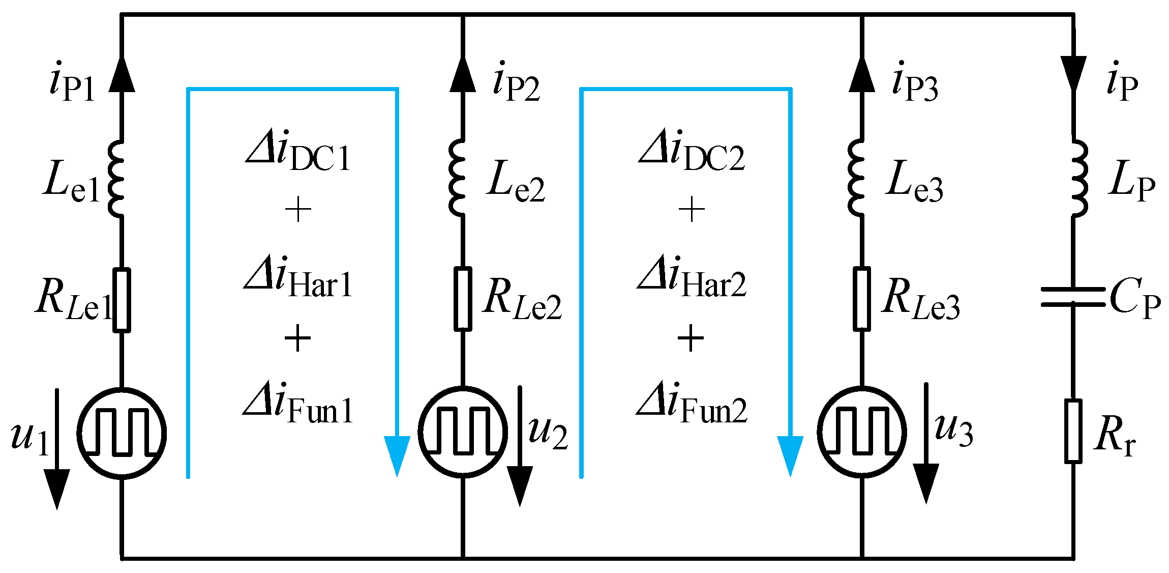
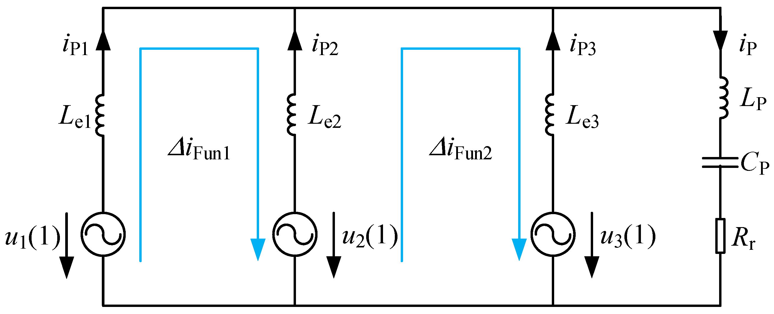
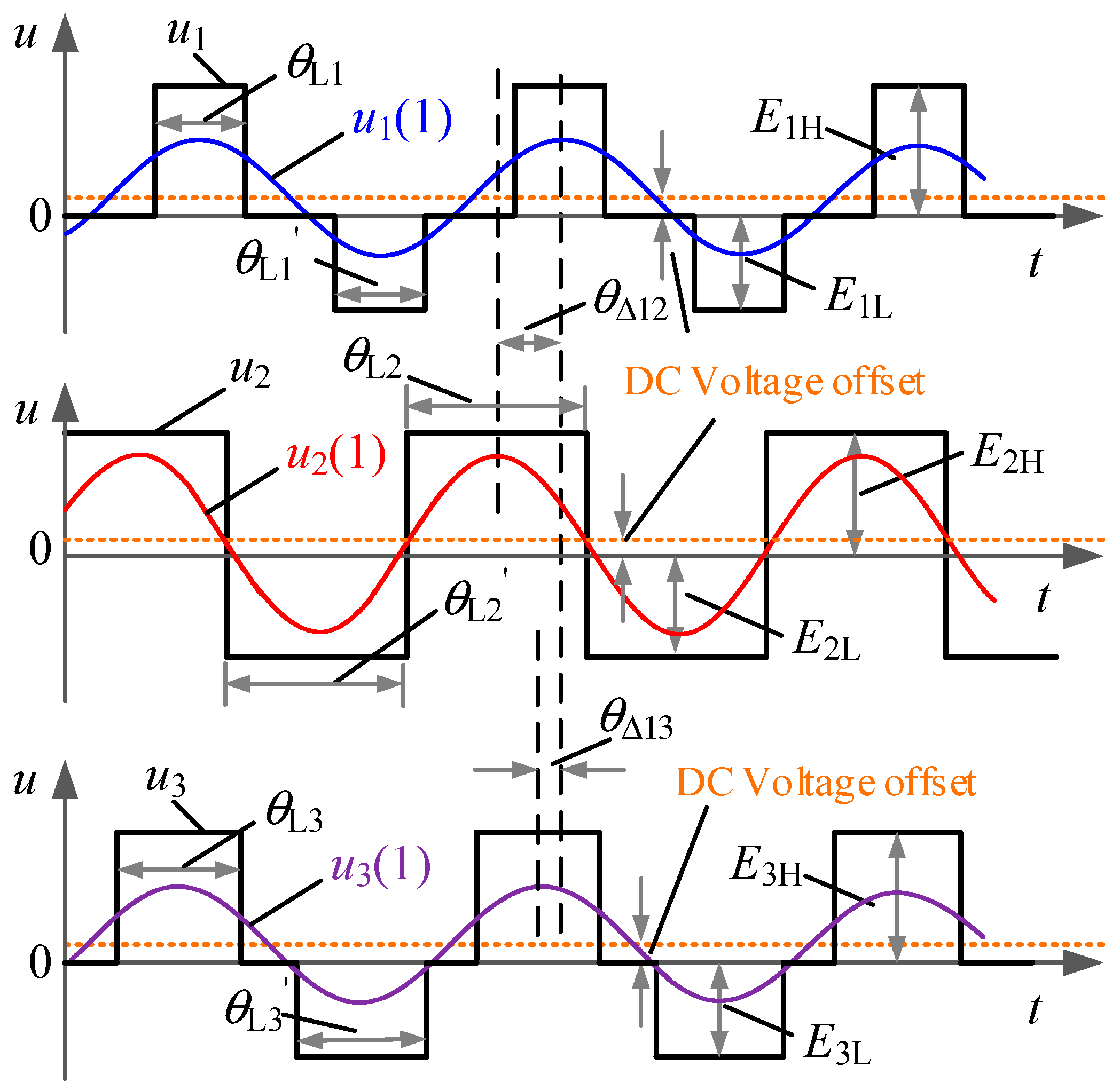
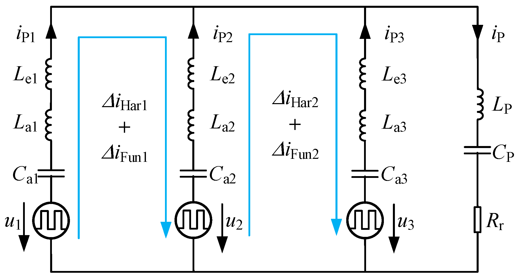
3. Analysis of the Fundamental Circulating Current

In practice, it is unlikely for the parallel unit to be identical. Generally speaking, the tolerance of the commercial inductor can be as high as 20%, and so is the capacitor [11]. For simplicity, assuming the series-parallel resonant tank is identical, only the tolerance of the connection inductors and the difference of the output inverter fundamental voltages are taken into consideration. According to Figure 5, based on the Kirchhoff’s voltage and current laws (KVL and KCL), we have:

$$\{\begin{array}{l}{\dot{U}}_1(1)=j\omega {\dot{I}}_{\mathrm{P}1}{L}_{\mathrm{e}1}+({\dot{I}}_{\mathrm{P}1}+{\dot{I}}_{\mathrm{P}2}+{\dot{I}}_{\mathrm{P}3})(R_{\mathrm{r}}+j\omega L_{\mathrm{P}}+\frac{1}{j\omega C_{\mathrm{P}}})\\ {\dot{U}}_2(1)=j\omega {\dot{I}}_{\mathrm{P}2}{L}_{\mathrm{e}2}+({\dot{I}}_{\mathrm{P}1}+{\dot{I}}_{\mathrm{P}2}+{\dot{I}}_{\mathrm{P}3})(R_{\mathrm{r}}+j\omega L_{\mathrm{P}}+\frac{1}{j\omega C_{\mathrm{P}}})\\ {\dot{U}}_3(1)=j\omega {\dot{I}}_{\mathrm{P}3}{L}_{\mathrm{e}3}+({\dot{I}}_{\mathrm{P}1}+{\dot{I}}_{\mathrm{P}2}+{\dot{I}}_{\mathrm{P}3})(R_{\mathrm{r}}+j\omega L_{\mathrm{P}}+\frac{1}{j\omega C_{\mathrm{P}}})\\ 0=j\omega L_{\mathrm{P}}+\frac{1}{j\omega C_{\mathrm{P}}}\end{array}$$

(6)

The branch currents can be derived by:

$$\{\begin{array}{c}{\dot{I}}_{\mathrm{P}1}=\frac{R_{\mathrm{r}}{L}_{\mathrm{e}2}({\dot{U}}_1(1)-{\dot{U}}_3(1))+R_{\mathrm{r}}{L}_{\mathrm{e}3}({\dot{U}}_1(1)-{\dot{U}}_2(1))+j\omega L_{\mathrm{e}2}{L}_{\mathrm{e}3}{\dot{U}}_1(1)}{j\omega R_{\mathrm{r}}(L_{\mathrm{e}1}{L}_{\mathrm{e}2}+L_{\mathrm{e}2}{L}_{\mathrm{e}3}+L_{\mathrm{e}1}{L}_{\mathrm{e}3})-{\omega }^2{L}_{\mathrm{e}1}{L}_{\mathrm{e}2}{L}_{\mathrm{e}3}}\\ {\dot{I}}_{\mathrm{P}2}=\frac{R_{\mathrm{r}}{L}_{\mathrm{e}1}({\dot{U}}_2(1)-{\dot{U}}_3(1))+R_{\mathrm{r}}{L}_{\mathrm{e}3}({\dot{U}}_2(1)-{\dot{U}}_1(1))+j\omega L_{\mathrm{e}1}{L}_{\mathrm{e}3}{\dot{U}}_2(1)}{j\omega R_{\mathrm{r}}(L_{\mathrm{e}1}{L}_{\mathrm{e}2}+L_{\mathrm{e}2}{L}_{\mathrm{e}3}+L_{\mathrm{e}1}{L}_{\mathrm{e}3})-{\omega }^2{L}_{\mathrm{e}1}{L}_{\mathrm{e}2}{L}_{\mathrm{e}3}}\\ {\dot{I}}_{\mathrm{P}3}=\frac{R_{\mathrm{r}}{L}_{\mathrm{e}1}({\dot{U}}_3(1)-{\dot{U}}_2(1))+R_{\mathrm{r}}{L}_{\mathrm{e}2}({\dot{U}}_3(1)-{\dot{U}}_1(1))+j\omega L_{\mathrm{e}1}{L}_{\mathrm{e}2}{\dot{U}}_3(1)}{j\omega R_{\mathrm{r}}(L_{\mathrm{e}1}{L}_{\mathrm{e}2}+L_{\mathrm{e}2}{L}_{\mathrm{e}3}+L_{\mathrm{e}1}{L}_{\mathrm{e}3})-{\omega }^2{L}_{\mathrm{e}1}{L}_{\mathrm{e}2}{L}_{\mathrm{e}3}}\end{array}$$

(7)

For n-module inverter IPT system, the kth circulating current is defined to be half of the current difference of module currents between module k and (k + 1) according to [11]:

$$\Delta {\dot{I}}_k=\frac{{\dot{I}}_{\mathrm{P}k}-{\dot{I}}_{\mathrm{P}(k+1)}}{2}$$

(8)

When n = 3, the circulating currents are $\Delta {\dot{I}}_1$ and $\Delta {\dot{I}}_2$.

Case 1: according to Equations (7) and (8), let $L_{\mathrm{e}1}=L_{\mathrm{e}2}=L_{\mathrm{e}3}=L_{\mathrm{e}}$ and ${\dot{U}}_1(1)\ne {\dot{U}}_2(1)\ne {\dot{U}}_3(1)$, the equation of the circulating currents are given by:

$$\{\begin{array}{l}\Delta {\dot{I}}_1=\frac{{\dot{I}}_{\mathrm{P}1}-{\dot{I}}_{\mathrm{P}2}}{2}=\frac{{\dot{U}}_1(1)-{\dot{U}}_2(1)}{j2\omega L_{\mathrm{e}}}\\ \Delta {\dot{I}}_2=\frac{{\dot{I}}_{\mathrm{P}2}-{\dot{I}}_{\mathrm{P}3}}{2}=\frac{{\dot{U}}_2(1)-{\dot{U}}_3(1)}{j2\omega L_{\mathrm{e}}}\end{array}$$

(9)

It can be concluded from Equation (9) that when ${\dot{U}}_1(1)\ne {\dot{U}}_2(1)\ne {\dot{U}}_3(1)$, the circulating currents exist, $\Delta {\dot{I}}_1\ne 0$, $\Delta {\dot{I}}_2\ne 0$.

Case 2: according to Equations (7) and (8), let $L_{\mathrm{e}1}\ne L_{\mathrm{e}2}\ne L_{\mathrm{e}3}$ and ${\dot{U}}_1(1)={\dot{U}}_2(1)={\dot{U}}_3(1)=\dot{U}(1)$, the equation of the circulating currents are derived as:

$$\{\begin{array}{l}\Delta {\dot{I}}_1=\frac{{\dot{I}}_{\mathrm{P}1}-{\dot{I}}_{\mathrm{P}2}}{2}=\frac{R_{\mathrm{r}}{L}_{\mathrm{e}3}\dot{U}(1)(L_{\mathrm{e}1}-L_{\mathrm{e}2})(L_{\mathrm{e}1}{L}_{\mathrm{e}2}+L_{\mathrm{e}1}{L}_{\mathrm{e}3}+L_{\mathrm{e}2}{L}_{\mathrm{e}3})}{2{[j{R}_{\mathrm{r}}(L_{\mathrm{e}1}{L}_{\mathrm{e}2}+L_{\mathrm{e}1}{L}_{\mathrm{e}3}+L_{\mathrm{e}2}{L}_{\mathrm{e}3})-\omega L_{\mathrm{e}1}{L}_{\mathrm{e}2}{L}_{\mathrm{e}3}]}^2}\\ \Delta {\dot{I}}_2=\frac{{\dot{I}}_{\mathrm{P}2}-{\dot{I}}_{\mathrm{P}3}}{2}=\frac{R_{\mathrm{r}}{L}_{\mathrm{e}1}\dot{U}(1)(L_{\mathrm{e}2}-L_{\mathrm{e}3})(L_{\mathrm{e}1}{L}_{\mathrm{e}2}+L_{\mathrm{e}1}{L}_{\mathrm{e}3}+L_{\mathrm{e}2}{L}_{\mathrm{e}3})}{2{[j{R}_{\mathrm{r}}(L_{\mathrm{e}1}{L}_{\mathrm{e}2}+L_{\mathrm{e}1}{L}_{\mathrm{e}3}+L_{\mathrm{e}2}{L}_{\mathrm{e}3})-\omega L_{\mathrm{e}1}{L}_{\mathrm{e}2}{L}_{\mathrm{e}3}]}^2}\end{array}$$

(10)

According to Equation (10), we can get that when $L_{\mathrm{e}1}\ne L_{\mathrm{e}2}\ne L_{\mathrm{e}3}$, the circulating currents exist too, $\Delta {\dot{I}}_1\ne 0$, $\Delta {\dot{I}}_2\ne 0$. From case 1 and case 2 analyzed above, we can draw a conclusion that the tolerance of the connection inductors or the difference of the output inverter fundamental voltages can cause the circulating currents. Without loss of generality, for the n-module inverter IPT system, the circulating currents exist, $\Delta {\dot{I}}_1\ne 0$, $\Delta {\dot{I}}_2\ne 0$, … $\Delta {\dot{I}}_{n-1}\ne 0$.

4. Analysis of a Current Decomposed Method and Control Diagram

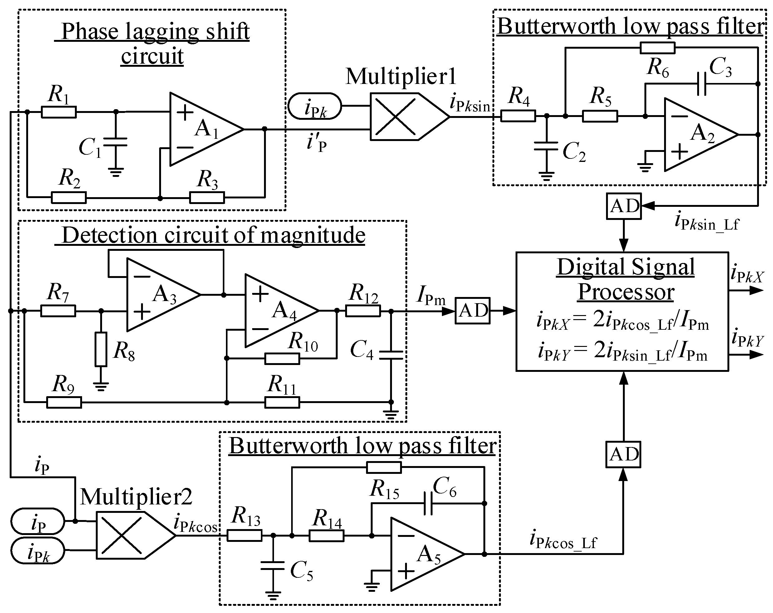
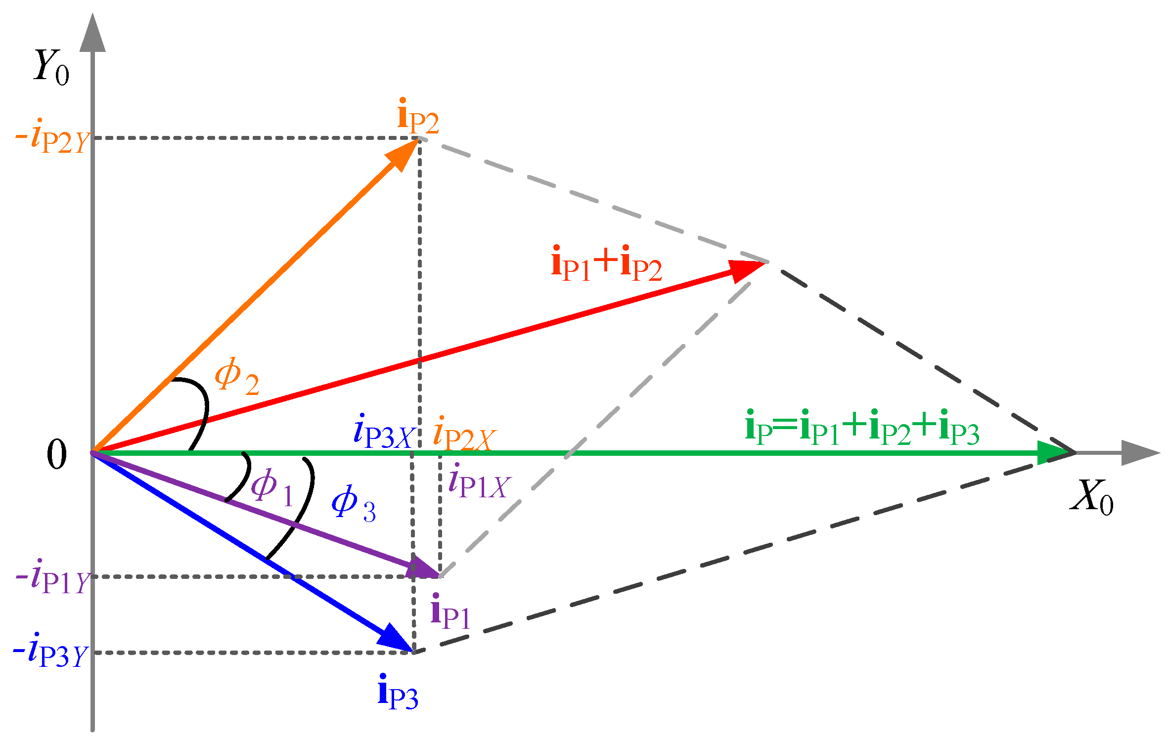
4.1. Current Decomposition

In order to reduce the fundamental circulating current, phasor differences between branch currents should be controlled as small as possible. Therefore, a current phasor control strategy based on the current decomposing method is applied in the parallel-connected inverter IPT system. In order to obtain the phasor of each branch current, a novel decomposition method will be analyzed in detail in this section. With the current decomposing method analyzed in this section, the high frequency AC signals can be transformed to DC signals for the phasor controllers, which decreases the computational burden and complexity of the control algorithm. Here, we set the primary coil current as reference, and it can be defined as:

$$i_{\mathrm{P}}=I_{\mathrm{Pm}}\cos (\omega t)$$

(11)

where $I_{\mathrm{Pm}}$ is the magnitude of the primary coil current. By employing a phase lagging shift circuit, the orthogonal signal can be generated from the reference current i_P:

$${i_{\mathrm{P}}}^{\prime }=I_{\mathrm{Pm}}\sin (\omega t)$$

(12)

Hence, the orthogonal frame can be derived by:

$$\{\begin{array}{l}{X}_0=i_{\mathrm{P}}=I_{\mathrm{Pm}}\cos (\omega t)\\ Y_0={i_{\mathrm{P}}}^{\prime }=I_{\mathrm{Pm}}\sin (\omega t)\end{array}$$

(13)

Herein, the branch current of each parallel unit is defined by:

$${i_{\mathrm{P}}}_k=I_{\mathrm{P}k\mathrm{m}}\cos (\omega t+{\varphi }_k)=i_{\mathrm{P}kX}\cos (\omega t)+i_{\mathrm{P}kY}\sin (\omega t)$$

(14)

where:

$$\{\begin{array}{l}{i}_{\mathrm{P}kX}=I_{\mathrm{P}k\mathrm{m}}\cos ({\varphi }_k)\\ i_{\mathrm{P}kY}=-I_{\mathrm{P}k\mathrm{m}}\sin ({\varphi }_k)\end{array}$$

(15)

$i_{\mathrm{P}kX}$ and $i_{\mathrm{P}kY}$ are the real component and imaginary component of the branch current as per reference current. The magnitude of the branch current i_Pk is $I_{\mathrm{P}k\mathrm{m}}$, and the phase is ${\varphi }_k$, (k = 1, 2,…, n). The productions of Equation (13) by the kth inverter unit current $i_{\mathrm{P}k}$ can be expressed as:

$$\{\begin{array}{c}{i}_{\mathrm{P}k\cos }=I_{\mathrm{P}k\mathrm{m}}\cos (\omega t+{\varphi }_k)X_0=I_{\mathrm{Pm}}{I}_{\mathrm{P}k\mathrm{m}}\cos (\omega t+{\varphi }_k)\cos (\omega t)=\frac{I_{\mathrm{Pm}}{I}_{\mathrm{P}k\mathrm{m}}[\cos (2\omega t+{\varphi }_k)+\cos ({\varphi }_k)]}{2}\\ i_{\mathrm{P}k\sin }=I_{\mathrm{P}k\mathrm{m}}\cos (\omega t+{\varphi }_k)Y_0=I_{\mathrm{Pm}}{I}_{\mathrm{P}k\mathrm{m}}\cos (\omega t+{\varphi }_k)\sin (\omega t)=\frac{I_{\mathrm{Pm}}{I}_{\mathrm{P}k\mathrm{m}}[\sin (2\omega t+{\varphi }_k)-\sin ({\varphi }_k)]}{2}\end{array}$$

(16)

It can be seen from Equation (16) that both $i_{\mathrm{P}k\cos }$ and $i_{\mathrm{P}k\sin }$ are composed of DC components and second-order harmonic components. By applying a Low-Pass Filter (LPF), the second-order harmonic components can be filtered out. Then, we can get the DC components:

$$\{\begin{array}{c}{i}_{\mathrm{P}kX\_\mathrm{Lf}}=\frac{I_{\mathrm{Pm}}{I}_{\mathrm{P}k\mathrm{m}}\cos ({\varphi }_k)}{2}\\ i_{\mathrm{P}kY\_\mathrm{Lf}}=\frac{-I_{\mathrm{Pm}}{I}_{\mathrm{P}k\mathrm{m}}\sin ({\varphi }_k)}{2}\end{array}$$

(17)

With the magnitude of the primary coil current $I_{\mathrm{Pm}}$, the kth inverter unit current $i_{\mathrm{P}k}$ can be decomposed in the orthogonal frame, that is:

$$\{\begin{array}{c}{i}_{\mathrm{P}kX}=2i_{\mathrm{P}kX\_\mathrm{Lf}}/I_{\mathrm{P}\mathrm{m}}\\ i_{\mathrm{P}kY}=2i_{\mathrm{P}kY\_\mathrm{Lf}}/I_{\mathrm{P}\mathrm{m}}\end{array}$$

(18)

According to Equations (14) and (18), the high frequency AC current signals have been transformed to DC current signals without PLL, which decreases the computational burden and complexity of the control algorithm. The decomposition circuit of kth inverter unit current $i_{\mathrm{P}k}$ is shown in Figure 6.

For example, let n = 3, the branch current of the parallel unit can be decomposed as shown in Figure 7. The coordinate shown in the Figure 7 consisted of X₀ and Y₀ is a rectangular system. To make the branch current $i_{\mathrm{P}k}$ equal, the current decomposed components in the X₀ axis or in the Y₀ axis, respectively, should be regulated to be equal. Besides, the Y component separately for each of the converters needs to control to be zero according to Equations (17) and (18), when the phase ${\varphi }_k$ is zero (${i_{\mathrm{P}}}_{1X}={i_{\mathrm{P}}}_{2X}={i_{\mathrm{P}}}_{3X}$, ${i_{\mathrm{P}}}_{1Y}={i_{\mathrm{P}}}_{2Y}={i_{\mathrm{P}}}_{3Y}=0$). For n-module inverter IPT system, the number of the decomposition circuits shown in Figure 6 should be n. All of the branch currents should be regulated to be equal (${i_{\mathrm{P}}}_{1X}={i_{\mathrm{P}}}_{2X}={i_{\mathrm{P}}}_{3X}...={i_{\mathrm{P}}}_{nX}$, ${i_{\mathrm{P}}}_{1Y}={i_{\mathrm{P}}}_{2Y}={i_{\mathrm{P}}}_{3Y}...={i_{\mathrm{P}}}_{nY}=0$). As a result, the problem can be solved for any number of parallel connected inverters.

The phase lagging shift prototype is used to generate the orthogonal signal as Equation (13) shows. The operational amplifier LM6142 is employed in this paper for the A₁–A₅ shown in Figure 6. The phase difference between the input signal and the output signal (the lagging one) is set to be 90° by choosing the proper resistance R₁ and the capacitance C₁ in the phase lagging shift circuit, and the designed principle is $\omega R_1{C}_1=1$. For eliminating the 5% tolerance in C₁, the potentiometer R₁ which is adjustable is employed. The four quadrant analog multiplier MLT04 is employed to realize the multiplication of Equation (16). The butterworth low pass filter is designed to filter out the second-order harmonic components shown in Equation (16), and the cut off frequency of the filter is 80 Hz. It may take 20–30 periods to filter out the second-order harmonic components for the filter and the DC components can be get as shown in Equation (17). However, for the low frequency application e.g., PV plants, the proposed approach may not be good enough. Because the operating frequency of the system is 50 Hz/60 Hz which is so closed to 0 Hz. As a result, it takes more time to filter out the second-order harmonic components and it is difficult to get the DC components for the controllers. The parameters of the decomposition circuit shown in Figure 6 are listed in

Table 1. Design specifications and parameters of the decomposition circuit.

Parameters	Value
The resistance of R2, R3, R7, R8/kΩ	10
The resistance of R1/Ω	995.2
The resistance of R4, R6, R13, R15/kΩ	2.16
The resistance of R5, R14/kΩ	1.03
The resistance of R9, R10/kΩ	2
The resistance of R11/kΩ	1
The resistance of R12/kΩ	4.7
The capacitance of C1/nF	8
The capacitance of C2, C5/uF	2.67
The capacitance of C3, C6/uF	1
The capacitance of C4/uF	10
Multiplier 1 and 2: MLT04
Operational amplifier A1–A5: LM6142

.

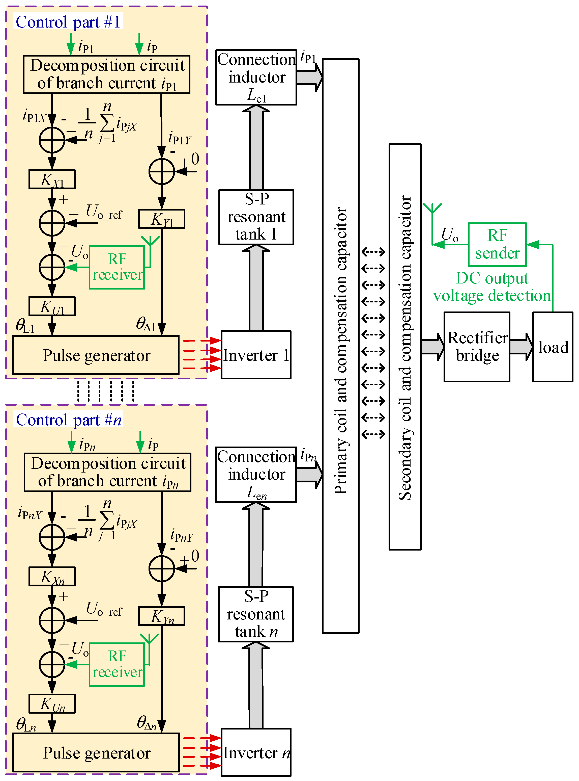
4.2. Control Diagram

The control block diagram of the proposed algorithm is shown in Figure 8. Firstly, by employing the decomposition circuit as show in Figure 6, the kth branch current $i_{\mathrm{P}k}$ can be decomposed into two DC components, i_PkX and i_PkY. Secondly, the current decomposed component in the X₀ axis i_PkX, is used for the magnitude sharing control loop of the kth inverter. In addition, the current decomposed component in the Y₀ axis i_PkY, is used for the phase difference minimized control loop of the kth inverter unit current $i_{\mathrm{P}k}$. Generally speaking, the received high frequency AC voltage of the secondary side cannot be used directly, but the rectifier converts it into a DC voltage for the load. As a result, the load voltage U_o is detected and sent to the primary side control parts via radio frequency (RF) [33]. However, in the field of the PV plants, the frequency and the magnitude of the bus voltage achieved by PLL [34] are needed for regulating the output power. It is difficult to add the output voltage regulation parts in the control diagram to replace the load voltage U_o as shown in the Figure 8.

With the i_PkX, i_PkY and U_o, the proportion integration (PI) controller can yield the conduction angle ${\theta }_{\mathrm{L}k}$ and phase ${\theta }_{\Delta k}$, which is used to generate the pulse width for the kth inverter to reduce the circulating currents and keep the output voltage constant. K_Xk is the X component of the branch current sharing PI controller. K_Uk is the voltage feedback PI controller. K_Yk is the Y component of the branch current minimizing PI controller. All of the controllers presented in the paper are designed as digital PI controllers with incremental PI algorithm which can well follow the reference signal. The equation of the incremental PI algorithm is:

$$\begin{array}{cc}\hfill \Delta u_k& =K_P[e_k-e_{k-1}+\frac{T}{T_I}{e}_k+\frac{T_D}{T}(e_k-2e_{k-1}+e_{k-2})]\hfill \\ & =K_P(1+\frac{T}{T_I}+\frac{T_D}{T})e_k-K_P(1+\frac{2T_D}{T})e_{k-1}+K_P\frac{T_D}{T}{e}_{k-2}\hfill \\ & =\alpha e_k+\beta e_{k-1}+\gamma e_{k-2}\hfill \end{array}$$

(19)

where $\alpha =K_P(1+\frac{T}{T_I}+\frac{T_D}{T})$, $\beta =-K_P(1+\frac{2T_D}{T})$, $\gamma =K_P\frac{T_D}{T}$, T is the sampling period, and $e_k$ is the error between the kth sampling value and the (k − 1)th sampling value. For the industrial application, the values of the $\alpha$, $\beta$, $\gamma$ for the PI controllers have been achieved by observing the experimental phenomena and debugging experience. Finally, we can get a relatively optimal values of the $\alpha$, $\beta$, $\gamma$ for the PI controllers which can well follow the reference when there is a fast variation. The performance of the PI controllers are verified in the following section. Furthermore, we will take faster controllers into consideration, e.g., robust controller, sliding mode controller and so on to follow the reference, when there is a faster variation.

Finally, the parallel-connected inverter IPT system will work under the condition that, the magnitudes of the branch currents are controlled to be identical, the current phase differences between the parallel units are zero, and the load voltage U_o is equal to the reference voltage U_{o_ref}.

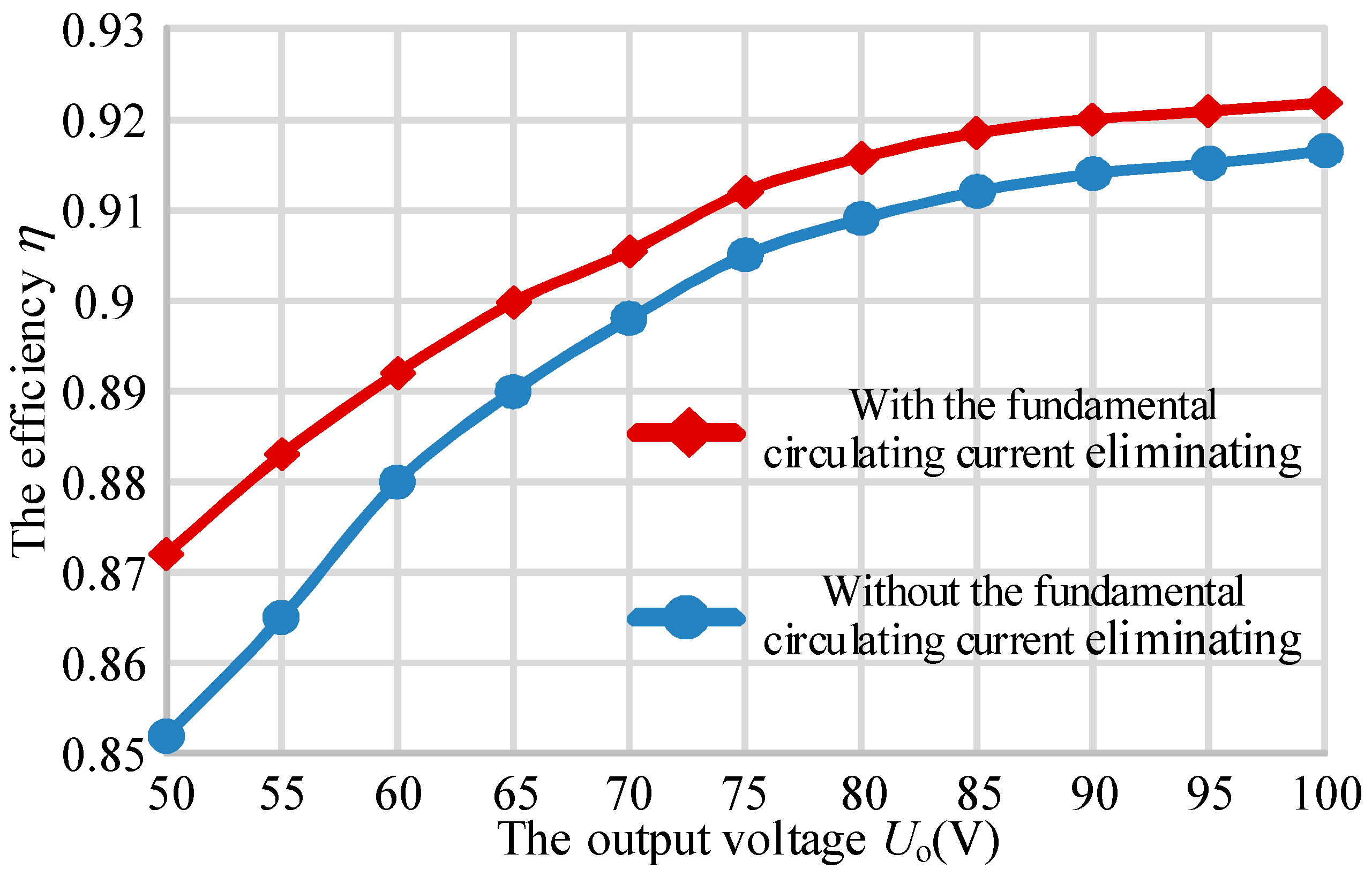
5. Experimental Results

In order to verify the proposed current phasor and voltage constant control approach, an experimental IPT prototype is set up with two identical units connected in parallel without loss of generality. The maximum output power of this prototype is 1 kW. By regulating the conduction and phase angles of the parallel inverter output voltages, the circulating currents can be reduced, and the output voltage can be controlled constantly.

The exterior appearance of the experimental setup is portrayed in Figure 9 and the circuit parameters of the prototype are listed in

Table 2. Design specifications and circuit parameters of inductive power transfer (IPT) prototype.

Parameters	Value
Inverter frequency f/kHz	20
Inductance of inverter 1 in series La1/μH	445.0
Capacitance of inverter 1 in series Ca1/nF	143.3
Inductance of inverter 1 in parallel Lb1/μH	42.7
Capacitance of inverter 1 in parallel Cb1/nF	1476.0
The connection inductance of inverter 1 Le1/μH	60.9
Inductance of inverter 2 in series La2/μH	432.8
Capacitance of inverter 2 in series Ca2/nF	147.0
Inductance of inverter 2 in parallel Lb2/μH	43.6
Capacitance of inverter 2 in parallel Cb2/nF	1472.0
The connection inductance of inverter 2 Le2/μH	39.2
Inductance of the primary coil LP/μH	195.0
Capacitance of primary circuit CP/nF	323.7
Mutual inductance M/μH	60.0
The air gap of the primary and secondary coils d/cm	12
Inductance of the secondary coil LS/μH	507.34
Capacitance of secondary circuit CS/nF	124.8
Equivalent resistance of the load RL/Ω	10
MOSFET: IRF640N
RF: nRF24L01

. The two inverters are separately powered by two isolated DC supplies. The TMS320F28335 digital signal processing (DSP) (Texas Instruments, Dallas, TX, USA) is employed as the controller of the IPT system, and generates gate pulse signals for the inverter switching devices. The experimental waveforms are measured and displayed by Agilent MSO-X 4034A scope (Agilent, Palo Alto, CA, USA).

From Section 3, it is clear that both the tolerance of the connection inductors and the difference of the output inverter fundamental voltages can cause the circulating currents. Considering the worst condition, we set the connection inductance $L_{\mathrm{e}1}\ne L_{\mathrm{e}2}$, and the output inverter fundamental voltages ${\dot{U}}_1(1)\ne {\dot{U}}_2(1)$, for validating the proposed current phasor control approach.

The connection inductance L_e1 = 1.2 L_e, L_e2 = 0.8 L_e, L_e = 50 μH, the input DC voltages E₁ = 1.15 E₂ = 115 V and the reference load output voltage U_{o_ref} = 100 V. The steady-state current waveforms without the current phasor control but with the constant voltage control are shown in Figure 10. By fixing the phase angles ${\theta }_{\Delta 1}={\theta }_{\Delta 2}=0$ and regulating the conduction angles (${\theta }_{\mathrm{L}1}$ = ${\theta }_{\mathrm{L}2}$), the output load voltage is controlled to be 100 V as same as the reference voltage U_{o_ref}. However, there is a large difference between the branch currents i_P1 and i_P2, which is shown in the bottom waveform of Figure 10 the magnitude of the twice circulating current is 5 A. With the output voltage and current ($U_{\mathrm{o}}$ and $I_{\mathrm{o}}$), the DC input voltages (E₁ and E₂), and the DC input currents (I₁ and I₂), the efficiency of the experiment can be calculated by equation $\eta =\raisebox{1ex}{$U_{\mathrm{o}}{I}_{\mathrm{o}}$}\!\left/ \!\raisebox{-1ex}{$(E_1{I}_1+E_2{I}_2)$}\right.=\frac{1008}{115.3\times 4.69+100.2\times 5.58}\approx 91.65\%$. The output power is 1 kW and the efficiency is 91.65%. Fortunately, no DC or harmonic circulating current exists, owing to the employment of the series-parallel resonant tank.

With the current phasor and constant voltage control approach applied into the IPT prototype, the circulating current between the branch currents i_P1 and i_P2 can be reduced effectively, and the output load voltage is controlled to be 100 V. The steady-state current waveforms are shown in Figure 11. The magnitude of the twice circulating current is less than 0.5 A, which is near one-tenth of that without the current phasor control. The efficiency of the experiment can be calculated by the equation$\eta =\raisebox{1ex}{$U_{\mathrm{o}}{I}_{\mathrm{o}}$}\!\left/ \!\raisebox{-1ex}{$(E_1{I}_1+E_2{I}_2)$}\right.=\frac{1011}{115.3\times 4.75+100.2\times 5.48}\approx 92.18\%$. At the same output power (about 1 kW), the efficiency is 92.18% and is higher than that without the current phasor control (91.65%). In order to justify the statement, an efficiency comparison for the different operating point is provided in Figure 12. At the same time, no DC or harmonic circulating current exists. The experimental results verify the performance of the proposed current phasor and constant voltage control approach, which is suitable for the parallel-connected inverter IPT system.

The dynamic performance during the output voltage transient is shown in Figure 13. When the reference voltage U_{o_ref} is stepped up from 80 to 100 V, U_o rises up quickly. The response time is about 24 ms, and there is no overshoot of the output voltage. When the reference voltage U_{o_ref} is stepped down from 100 to 80 V, U_o drops immediately. The response time is about 18 ms, and there is no overshoot of the output voltage too. The waveform of the output voltage is shown at the top of Figure 13. Meanwhile, the branch currents (i_P1 and i_P2) and the primary coil i_P current are given in Figure 13.

The dynamic performance during the load transient is shown in Figure 14. When the load R_L is stepped down from 15 to 10 Ω, it takes a little response time (about 25 ms) to return to 100 V, and the overshoot of the output voltage U_o is small. When the load R_L is stepped up from 10 to 15 Ω, it takes a bit of response time (about 20 ms) to return to 100 V, and the overshoot of the output voltage U_o is small too. The waveform of the output voltage is shown at the top of Figure 14. Meanwhile, the branch currents (i_P1 and i_P2) and the primary coil i_P current are given in Figure 14.

According to the experimental results mentioned above, it can be concluded that the proposed current phasor and constant voltage control approach has a good dynamic response performance with asymmetrical connection inductances and different DC input voltages.

6. Conclusions

A novel multiple inverters based IPT system has been described in this paper to upgrade the power capability of the IPT system by using low-power semiconductors. Series-parallel resonant tank is used to suppress the DC and harmonic components of the circulating current caused by a slight unbalance of the control signal, the inner resistances of the inverters and other uncertainties. The current decomposition based phasor control method has been proposed to eliminate the fundamental circulating current. With the current decomposing method, the high frequency AC signals can be transformed to DC signals for the phasor controllers, which decreases the computational burden and complexity of the control algorithm. It provides convenience for power extension through the coordination between multiple resonant inverter units and the current decomposing circuits which reduces the manufacturing cost. Finally, a 1-kW parallel two-inverter IPT prototype has been conducted to verify the performance of the proposed control method. The experimental results demonstrate that the proposed current phasor and voltage constant control approach can reduce the fundamental circulating currents effectively and own a good dynamic performance.

References

1. Boys, J.T.; Covic, G.A.; Green, A.W. Stability and control of inductively coupled power transfer systems. IEE Proc. Electr. Power Appl. 2000, 147, 37–43. [Google Scholar] [CrossRef]
2. Aditya, K.; Williamson, S. Linearization and control of series-series compensated inductive power transfer system based on extended describing function concept. Energies 2016, 9, 962. [Google Scholar] [CrossRef]
3. Li, Y.L.; Sun, Y.; Dai, X. μ-Synthesis for frequency uncertainty of the ICPT system. IEEE Trans. Ind. Electron. 2013, 60, 291–300. [Google Scholar] [CrossRef]
4. Wen, F.; Huang, X. Optimal magnetic field shielding method by metallic sheets in wireless power transfer system. Energies 2016, 9, 733. [Google Scholar] [CrossRef]
5. Zaheer, A.; Kacprzak, D.; Covic, G.A. A bipolar receiver pad in a lumped IPT system for electric vehicle charging applications. In Proceedings of the 2012 IEEE Energy Conversion Congress and Exposition (ECCE), Raleigh, NC, USA, 15–20 September 2012; pp. 283–290.
6. Huh, J.; Lee, S.W.; Lee, W.Y.; Cho, G.H.; Rim, C.T. Narrow-width inductive power transfer system for online electrical vehicles. IEEE Trans. Power Electron. 2011, 26, 3666–3679. [Google Scholar] [CrossRef]
7. Miller, J.M.; Jones, P.T.; Li, J.M.; Onar, O.C. ORNL experience and challenges facing dynamic wireless power charging of EV’s. IEEE Circuits Syst. Mag. 2015, 15, 40–53. [Google Scholar] [CrossRef]
8. Kim, S.; Park, H.H.; Kim, J.; Ahn, S. Design and analysis of a resonant reactive shield for a wireless power electric vehicle. IEEE Trans. Microw. Theory Tech. 2014, 62, 1057–1066. [Google Scholar] [CrossRef]
9. Lee, J.Y.; Yoo, K.M.; Jung, B.S.; Chae, B.S.; Seo, J.K. Large air-gap 6.6 kW wireless EV charger with self-resonant PWM. Electron. Lett. 2014, 50, 459–461. [Google Scholar] [CrossRef]
10. Hao, H.; Covic, G.A.; Boys, J.T. A parallel topology for inductive power transfer power supplies. IEEE Trans. Power Electron. 2014, 29, 1140–1151. [Google Scholar] [CrossRef]
11. Ye, Z.; Jain, P.K.; Sen, P.C. Circulating current minimization in high-frequency AC power distribution architecture with multiple inverter modules operated in parallel. IEEE Trans. Ind. Electron. 2007, 54, 2673–2687. [Google Scholar]
12. Borrega, M.; Marroyo, L.; Gonzalez, R.; Balda, J.; Agorreta, J.L. Modeling and control of a master–slave PV inverter with N-paralleled inverters and three-phase three-limb inductors. IEEE Trans. Power Electron. 2013, 28, 2842–2855. [Google Scholar] [CrossRef]
13. Mohammadpour, A.; Parsa, L.; Todorovic, M.H.; Lai, R.; Datta, R.; Garces, L. Series-Input parallel-output modular-phase DC–DC converter with soft-switching and high-frequency isolation. IEEE Trans. Power Electron. 2016, 31, 111–119. [Google Scholar] [CrossRef]
14. Namadmalan, A.; Moghani, J.S. Tunable self-oscillating switching technique for current source induction heating systems. IEEE Trans. Ind. Electron. 2014, 61, 2556–2563. [Google Scholar] [CrossRef]
15. Kim, J.H.; Lee, B.S.; Lee, J.H.; Lee, S.H.; Park, C.B.; Jung, S.M.; Baek, J. Development of 1-MW inductive power transfer system for a high-speed train. IEEE Trans. Ind. Electron. 2015, 62, 6242–6250. [Google Scholar] [CrossRef]
16. Miller, J.M.; Daga, A. Elements of wireless power transfer essential to high power charging of heavy duty vehicles. IEEE Trans. Transp. Electrification 2015, 1, 26–39. [Google Scholar] [CrossRef]
17. Li, Y.; Mai, R.K.; Lu, L.W.; He, Z.Y. Active and reactive currents decomposition based control of angle and magnitude of current for a parallel multi-inverter IPT system. IEEE Trans. Power Electron. 2017, 32, 1602–1614. [Google Scholar] [CrossRef]
18. Li, Y.; Mai, R.K.; Yang, M.K.; He, Z.Y. Cascaded multi-level inverter based IPT systems for high power applications. J. Power Electron. 2015, 15, 1508–1516. [Google Scholar] [CrossRef]
19. Li, Y.; Mai, R.K.; Lu, L.W.; He, Z.Y. A novel IPT system based on dual coupled primary tracks for high power applications. J. Power Electron. 2016, 16, 111–120. [Google Scholar] [CrossRef]
20. Li, Y.; Mai, R.; Lin, T.; Sun, H.; He, Z. A novel WPT system based on dual transmitters and dual receivers for high power applications: Analysis, design and implementation. Energies 2017, 10, 174. [Google Scholar] [CrossRef]
21. Mai, R.K.; Li, Y.; Lu, L.W.; He, Z.Y. A power regulation and harmonic current elimination approach of parallel multi-inverter for supplying IPT systems. J. Power Electron. 2016, 16, 1245–1255. [Google Scholar] [CrossRef]
22. Kawabata, T.; Higashino, S. Parallel operation of voltage source inverters. IEEE Trans. Ind. Appl. 1988, 24, 281–287. [Google Scholar] [CrossRef]
23. Zhang, Y.; Duan, S.; Kang, Y.; Chen, J. The restrain of harmonic circulating currents between parallel inverters. In Proceedings of the CES/IEEE 5th International Power Electronics and Motion Control Conference (IPEMC 2006), Shanghai, China, 14–16 August 2006; pp. 1–5.
24. Ye, Z.; Boroyevich, D.; Choi, J.Y.; Lee, F.C. Control of circulating current in two parallel three-phase boost rectifiers. IEEE Trans. Power Electron. 2002, 17, 609–615. [Google Scholar]
25. Chen, J.F.; Chu, C.L. Combination voltage-controlled and current-controlled PWM inverters for UPS parallel operation. IEEE Trans. Power Electron. 1995, 10, 547–558. [Google Scholar] [CrossRef]
26. Guerrero, J.M.; Hang, L.; Uceda, J. Control of distributed uninterruptible power supply systems. IEEE Trans. Ind. Electron. 2008, 55, 2845–2859. [Google Scholar] [CrossRef] [Green Version]
27. Kosaka, T.; Tanahashi, F.; Matsui, N.; Fujitsuna, M. Current zero cross detection-based position sensorless control of synchronous reluctance motors. In Proceedings of the 37th Industry Applications Society (IAS) Annual Meeting. Conference Record of the Industry Applications Conference, Pittsburgh, PA, USA, 13–18 October 2002; pp. 1610–1616.
28. Nedeljkovic, D.; Ambrozic, V.; Nastran, J.; Hudnik, D. Synchronization to the network without voltage zero-cross detection. In Proceedings of the 9th Mediterranean Electrotechnical Conference (MELECON’98), Tel-Aviv, Israel, 18–20 May 1998; pp. 1228–1232.
29. Ye, Z.; Lam, J.C.W.; Jain, P.K.; Sen, P.C. A robust one-cycle controlled full-bridge series-parallel resonant inverter for a high-frequency AC (HFAC) distribution system. IEEE Trans. Power Electron. 2007, 22, 2331–2343. [Google Scholar] [CrossRef]
30. Hu, A.P. Selected Resonant Converters for IPT Power Supplies. Ph.D. Thesis, University Auckland, Auckland, New Zealand, 2001. [Google Scholar]
31. Wei, X.; Zhu, G.; Lu, J.; Xu, X. Instantaneous current-sharing control scheme of multi-inverter modules in parallel based on virtual circulating impedance. IET Power Electron. 2016, 9, 960–968. [Google Scholar] [CrossRef]
32. Guerrero, J.M.; De Vicuna, L.G.; Matas, J.; Miret, J.; Castilla, M. Output impedance design of parallel-connected UPS inverters with wireless load-sharing control. IEEE Trans. Ind. Electron. 2005, 52, 1126–1135. [Google Scholar] [CrossRef]
33. Datasheetarchive. Available online: http://www.datasheetarchive.com/dl/Datasheets-UD1/DSAUD006800.pdf (accessed on 27 November 2016).
34. Yuan, J.; Gao, F.; Gao, H.; Zhang, H.; Wu, J. An adaptive control strategy for parallel operated photovoltaic inverters. In Proceedings of the Power Electronics and Motion Control Conference (IPEMC), Harbin, China, 2–5 June 2012; pp. 1522–1526.
Figure 1. The inductive power transfer (IPT) system based on parallel-connected inverter with the series-parallel resonant tank.
Energies 10 00261 g001
Figure 2. The equivalent circuit of the IPT system without the series-parallel resonant tank.
Energies 10 00261 g002
Figure 3. The output voltage waveforms of parallel two inverters.
Energies 10 00261 g003
Figure 4. The equivalent circuit of the IPT system with the series resonant tank.
Energies 10 00261 g004
Figure 5. The equivalent circuit of the IPT system with the series-parallel resonant tank.
Energies 10 00261 g005
Figure 6. The decomposition circuit of the kth inverter unit current i P k .
Energies 10 00261 g006
Figure 7. The decomposition of branch currents when n = 3.
Energies 10 00261 g007
Figure 8. The control block diagram.
Energies 10 00261 g008
Figure 9. The exterior appearance of the proposed IPT prototype.
Energies 10 00261 g009
Figure 10. The waveforms of Uo, iP1, iP2, iP and 2 Δ i without the current phasor control.
Energies 10 00261 g010
Figure 11. The waveforms of Uo, iP1, iP2, iP and 2 Δ i with the current phasor control.
Energies 10 00261 g011
Figure 12. An efficiency comparison for different operating point (at Uo = 50–100 V).
Energies 10 00261 g012
Figure 13. Close loop system response to step change in reference output load voltage from 80 to 100 V and then back to 80 V.
Energies 10 00261 g013
Figure 14. Close loop system response to step change of load resistance from 15 Ω to 10 Ω and then back to 15 Ω.
Energies 10 00261 g014