Signal-Based Gas Leakage Detection for Fluid Power Accumulators in Wind Turbines

Abstract

This paper describes the development and application of a signal-based fault detection method for identifying gas leakage in hydraulic accumulators used in wind turbines. The method uses Multiresolution Signal Decomposition (MSD) based on wavelets for feature extraction from a single fluid pressure measurement located close to the accumulator. Gas leakage is shown to create increased variations in this pressure signal. The Root Mean Square (RMS) of the detail coefficient Level 9 from the MSD is found as the most sensitive and robust fault indicator of gas leakage. The method is verified on an experimental setup allowing for the replication of the conditions for accumulators in wind turbines. Robustness is tested in a multi-fault environment where gas and external fluid leakage occurs simultaneously. In total, 24 experiments are performed, which show that the method is sensitive to gas leakage in the desired range and can be isolated from external fluid leakage. Additionally, the robustness to other operating conditions, such as wind speeds between rated and cut-off, turbulence intensity and ambient temperature is evaluated via simulations of a pitch system in a wind turbine using the Fatigue, Aerodynamics, Structures and Turbulence program (FAST). Simulation shows that robustness is affected at low ambient temperatures, however, detection is permitted in the range of 22–60 ${}^{\circ }\mathrm{C}$.

1. Introduction

Wind turbines operate as power plants by converting the kinetic energy of the wind to electric power. Because of the nature of their operation, wind turbines are typically designed with a safety system that shuts down power production in the event of a failure. Several studies have indicated that turbine availability is greatly reduced by down time caused by such failures [1,2,3,4]. One of the main safety measures typically installed in turbines is the pitch system, which rotates the blades along their longitudinal axis. If a critical failure occurs, the blades are turned out of the wind, which aerodynamically stops rotation. The pitch system is additionally used for adjusting the pitch angle to achieve a desired power output of the turbine. The main concern is that pitch systems represent one of the most unreliable subsystems of turbines [1,2].

Modern wind turbines employ either electrical or fluid power pitch systems. Fluid power pitch systems are preferred on offshore turbines, but generally, the distribution among the two types is equal [5]. In this paper, fluid power pitch systems are considered. Fluid power pitch systems drive the pitch angle using a linear extending or retracting cylinder. The cylinder movement is under normal conditions controlled by a proportional valve and pump. In the event of a critical failure, the cylinders must be brought to the fully-extended position. Emergency stop is performed by releasing pressurized fluid to the cylinders stored in hydraulic accumulators. Proper functioning of the accumulators is therefore essential to the safety of wind turbines. A recent study on offshore wind turbines indicates that accumulator faults account for over 10% of all pitch system failures [2]. Due to the high failure rate of accumulators and the safety critical function, failure analysis shows that accumulator gas leakage is amongst the highest risk factors of pitch systems [6].

The hydraulic accumulator is a device consisting of two chambers where one contains pressurized fluid and the other holds an inert gas, typically nitrogen. The gas is compressed as fluid enters the accumulator. Typical failure modes are related to either internal or external leakage of either the gas or fluid. External and internal gas leakage present a substantial portion of accumulator faults because of the low viscosity of the gas. Both internal and external gas leakage causes a decrease in ability to store energy, which in turn makes the pitch system unable to perform an emergency stop. It is therefore desirable to monitor gas leakages in hydraulic accumulators.

Generally, the amount of gas contained in the accumulator is estimated by measuring the gas pressure and temperature when the accumulator holds no fluid. This procedure is used when charging the accumulator with gas either at installation or during maintenance. To reduce the cost and the number of external leakage paths in the gas chamber, the gas pressure and temperature sensors are omitted under normal operation. Accumulators in pitch systems are, however, equipped with a pressure sensor on the fluid side. Among others, this sensor is used as a feedback for controlling the accumulator fluid pressure. The amount of gas may therefore be estimated by a combination of this pressure signal and knowledge of the current volume of fluid contained in the accumulator. For piston type accumulators, the fluid volume is directly proportional to the piston position. However, installing a position transducer in accumulators is impractical and expensive and adds leakage paths to either the fluid or gas chamber. Moreover, this solution is not suitable for bladder-type accumulators, which are also used in pitch systems. The motivation for the method presented in this paper is therefore based on the ability to detect accumulator gas leakage using only the existing sensors available in pitch systems.

In regard to prior work, the detection of accumulator faults in a pitch system was considered in a patent application by Nielsen et al. [7]. The accumulator function was evaluated by disconnecting it from the main circuit and letting it drain through an orifice to the tank. The fluid pressure was monitored during this procedure, and faults were detected by comparing the time it takes for the fluid to drain with a predetermined value. The proposed solution entails numerous additional components connected to a critical part of the pitch system. The failure of any of these components may therefore compromise the safety function of the pitch system. A similar method was proposed in a patent application by Minami et al. [8]. In this patent, it is not evident how the accumulator fluid is drained, but it was mentioned that the procedure is performed under conditions where the turbine is shut down. Thus, the accumulator function is not monitored during operation.

Despite the criticality of accumulator gas leakage, only a single research source has covered this topic. Helwig et al. [9] presented signal-based methods for detecting accumulator leakage and several other faults in an experimental setup using multiple sensors. The measured signals covered pressures, flows, temperatures and pump power. The most robust method for detecting accumulator gas leakage was shown to be obtained from a linear discriminant analysis of time domain features determined from the measured signals. Among others, the time domain features used where median, variance, skewness and kurtosis. While the method is promising for detecting gas leakage, it uses measurements of flow and several pressures, which are not normally present in pitch systems. Additionally, robustness was shown to decrease when the setup operated under pseudo-random conditions. Pitch systems operate under highly random conditions because of the stochastic load variations caused by the wind. Pfeffer et al. [10] developed a State of Charge (SoC) estimator for hydraulic accumulators using fluid pressure, temperature sensors and pump flow. The SoC is a measure of the fluid volume confined in the accumulator. The estimator was based on an Extended Kalman Filter (EKF) utilizing a simplified model of the accumulator. Gas leakage was not specifically covered, but the gas mass was presented as an output of the estimator. Experimental tests showed that the gas mass could be estimated with an error of approximately 3%. No results were presented on the precision in the presence of gas leakage.

In a more general context, an overview of fault detection methods related to fluid power pitch systems was presented in a review by Liniger et al. [11]. From this review, it is evident that much effort has gone into the detection and isolation of various types of cylinder leakage. Over the last few decades, the research was seen to shift in paradigm from model-based to signal-based fault detection. The efficiency of model-based methods is dependent on the model precision, which is challenged by the nonlinear behaviour and often large parameter variations associated with fluid power systems [12]. To include the nonlinear behaviour, An and Sepehri [13] studied a model-based EKF for detection of internal and external cylinder leakage using both chamber pressures and piston position. Goharrizi and Sepehri [14] showed that a lower level of internal leakage could be detected on a similar setup by a signal-based method using wavelets, thus removing the effort needed to develop a model. The method was augmented by the same authors for the detection of external actuator leakage [15]. On the same experimental setup, the lowest level of internal leakage was detected by the cross-correlation of chamber pressures [16].

The main contribution of this paper is the design and investigation of a signal-based method using only the accumulator fluid pressure sensor for detection of gas leakage in wind turbines. The signal-based method will be based on wavelets and extend on the work performed on cylinder leakage detection [14,15]. For the first time, the method will be verified on an experimental setup operating in a multi-fault environment considering both gas and fluid leakage. The setup is constructed for the replication of realistic conditions where the supply pressure and load flow is controlled in closed loop according to typical behaviour. The robustness of the method will also be investigated under various operating conditions considering the effect of wind speed, turbulence and ambient temperature using the wind turbine simulation software FAST (Fatigue, Aerodynamics, Structures and Turbulence program).

The paper is arranged as follows. Section 2 presents a description of the wind turbine and fluid power pitch system including the considered operating conditions. An analysis of the dynamical changes of the accumulator due to faults is given in Section 3. Section 4 presents the gas leakage detection method and an evaluation of robustness in relation to the considered operating conditions and other faults. Experimental validation of the method is given in Section 5. Lastly, a discussion and conclusions are found in Section 6 and Section 7, respectively.

2. Wind Turbine and Pitch System

The wind turbine simulation model used in this study is based on the NREL 5 MW turbine implementation in the open source software FAST [17,18]. The configuration is a standard upwind three bladed variable speed variable pitch wind turbine with its specifications given in

Table 1. Main data for the wind turbine and pitch system simulation model.

FAST Data	Value
Nominal power	5 (MW)
Nominal hub speed	12 (RPM)
Tower height	90 (m)
Blade length (hub centre to tip)	63 (m)
Wind speed rating (cut-in/Nom./cut-off)	5/11.4/25 (m/s)
Turbulence model	Normal turbulence model
Pitch System Data
Pitch cylinder dim. (rod/piston/stroke)	Ø90/Ø140/1350 (mm)
Pump flow ($q_p$)	20 (L/min)
Accumulator capacity ($V_a$)	50 (L)
Accumulator dim. (piston/stroke)	Ø200/1600 (mm)

.

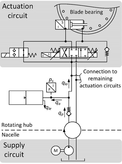
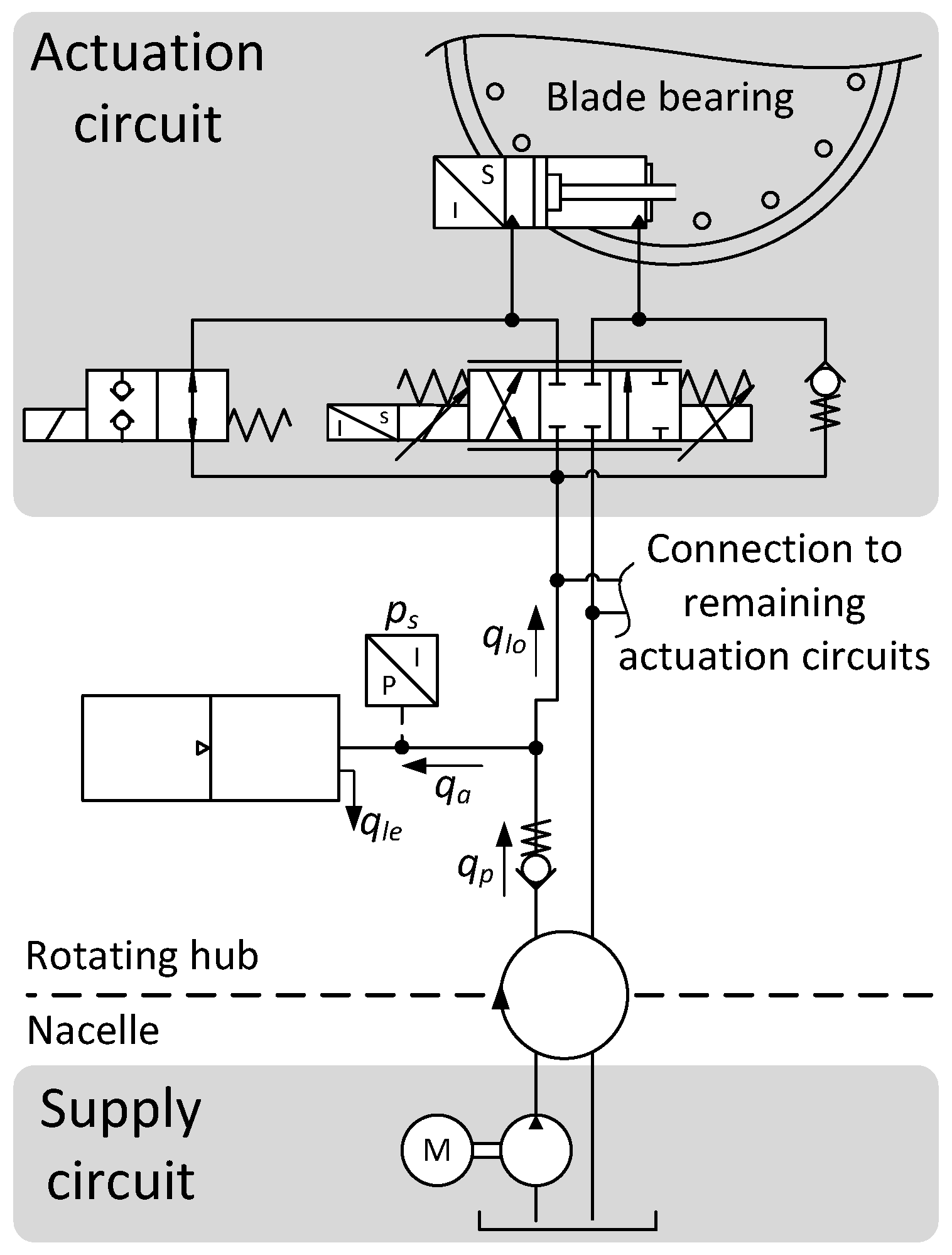
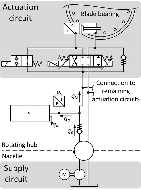
The model considers various dynamic effects like the elastic behaviour of the structural elements and wind turbulence. The model utilizes a three-dimensional wind flow field that affects the wind turbine during simulation. The flow field is generated by TurbSim [19]. Figure 1 shows the pitch system layout. The supply circuit is located in the nacelle of the wind turbine. It is therefore stationary to the rotating hub in which the three actuation circuits are located and connected to the blades. The actuation circuit enables control of the blade angle where the proportional valve is used in normal operation. In the event of a severe fault, the safety valve opens and connects the accumulator to both cylinder chambers. The cylinder thereby extends due to the regenerative configuration. As described in the Introduction, the blades act as an aerodynamic brake when the pitch cylinders are fully extended, which stops rotation of the hub.

The supply circuit is common to the three actuation circuits. The fluid is pressurized by a fixed displacement pump, which is activated when the supply pressure signal, $p_s$, drops below a preset lower limit. The pump is deactivated when the supply pressure reaches an upper limit. The upper and lower limits used in this study are 200 and 170 bar, respectively. The simulation model of the fluid power pitch system is based on the work by Pedersen et al. [20]. The pitch system model is implemented in MATLAB Simulink and co-simulated with FAST. The model considers the compressibility of fluid in the cylinder chambers, proportional valve dynamics and kinematics of the blade-cylinder coupling. The pitch angle control is governed by a gain scheduled PI-controller.

Operating Conditions

A range of operating conditions for the wind turbine is selected to analyse the effect in relation to the fault detection method. In this study, three representative operating conditions are selected: the mean wind speed, turbulence intensity and ambient temperature.

The wind speed and turbulence determines both the pitch angle reference and external loads to the pitch cylinder. In turn, a change in either pitch reference or external load affects the supply pressure, which is used for fault detection of the accumulator. It is therefore important to consider the effect of wind speed and turbulence. The wind conditions are based on the Design Load Case (DLC) 1.2 given in wind turbine design standard IEC 61400-1 [21]. DLC 1.2 is used when analysing turbine fatigue loads and is an indicator of normal operation. The wind conditions are site specific and defined by the mean wind speed at hub height and turbulence intensity class. The mean wind speeds considered are 11.4, 13 and 19 m/s. All mean wind speeds are selected above rated and below cut-off at 25 m/s. Simulation has shown that pitch activity and thus supply pressure changes are very small below rated wind speed, thus the lower limit. Simulation has also shown that instantaneous wind speeds at some points exceeds cut-off at 25 m/s for a mean wind speed above 19 m/s. This leads the turbine to shut down by fully pitching the blades out of the wind. This behaviour greatly affects the supply pressure due to a large flow demand when the cylinders are fully extended. The analysis and detection are therefore performed for wind speeds from rated to cut-off when the turbine is in continuous operation, which is a common operating point.

The turbulence intensity class is defined in three levels: high (A, 16%), medium (B, 14%) or low (C, 12%). The medium (B) level has been omitted, and only the extreme values are used.

The ambient temperature effects the dynamics of the gas contained in the accumulator. To account for this effect, the ambient temperatures used in simulations are −20, 0, 22, 60 ${}^{\circ }\mathrm{C}$. The ambient temperature range is selected from the extreme environmental conditions stated by the IEC 61400-1.

If not otherwise specified, the nominal operating condition is used in this paper. The nominal operating condition is defined as follows: mean wind speed 11.4 m/s, turbulence intensity Class A and ambient temperature 22 ${}^{\circ }\mathrm{C}$.

3. Accumulator Modelling and Fault Analysis

In this section, a model of the piston accumulator is developed, and it is shown how the considered faults affect the system. While the objective of the presented method is to detect gas leakage, it is interesting to evaluate the robustness to another commonly-occurring fault, namely external fluid leakage. External leakage is therefore included in the model to evaluate detection performance in a multi-fault environment.

Gas leakage can occur both externally and internally. Both faults are considered to have same influence on the accumulator, because gas leaking internally is assumed to be contained in the fluid and transported to the reservoir where it dissipates to the surroundings. Gas leakage may be regarded as a slow process, and it is normal to consider the amount of remaining gas in the accumulator instead of the leakage itself. In most applications, the pre-charge pressure is used as a measure instead of the gas mass, and this notation is also used throughout this paper. The considered pre-charge pressure range is given in

Table 2. Main data for the considered faults.

Fault	Measure	Value	Condition
Gas leakage	$p_{pc}$	180–50 (bar)	Pre-charge temperature
			$T_{pc}=22$${(}^{\circ }\mathrm{C})$
External fluid leakage	$q_{le}$	Zero/low/high	Supply pressure
		0/0.05/1 (L/min)	$p_s=200$ (bar)

. The lowest allowable level of pre-charge pressure is dependent on the turbine configuration, but a value of 50–70 bar is normally used. Note that the pre-charge pressure is temperature dependent. In this paper, all pre-charge pressures are evaluated at a gas temperature of 22 ${}^{\circ }\mathrm{C}$.

External fluid leakage is assumed to be laminar, i.e., proportional to the supply pressure. The leakage flow is characterized as either zero, low or high. The values are seen in Table 2.

3.1. Accumulator Model

The notation and positive flow definitions used are seen in Figure 1. Three governing equations are used for describing the accumulator dynamics: the continuity equation for the fluid, the equation of state for the gas and the energy balance of the gas. The stiffness of the fluid contained in the accumulator is orders of magnitude higher than the gas and is therefore neglected. Furthermore, the piston mass and friction are neglected in the following. These assumptions yield equal supply and gas pressure.

The continuity flow equation for the accumulator is given below in Equation (1). Here, the external fluid leakage, $q_{le}=k_{le}{p}_s$, is assumed to be laminar with a flow constant $k_{le}$. The accumulator flow is given by $q_a$. ${\dot{V}}_g$ denote the time derivative of the gas volume. In this paper, the “$\dot{}$” is further used for the time derivative of variables.

$$\begin{array}{c}\hfill {\dot{V}}_g=-q_a=q_{lo}-q_p+k_{le}{p}_s\end{array}$$

(1)

The main focus in the previous studies on accumulators has been on modelling the gas behaviour [22,23,24,25,26]. Otis and Pourmovahed [22] concluded that simplifying assumptions, such as ideal gas and adiabatic behaviour, are not appropriate in most applications where steel accumulators are used. To describe the real behaviour of the gas, good results are obtained by using the Benedict-Webb-Rubin (BWR) equation of state [22,25]. The equation of state describes the relation between the pressure $p_s$, volume $V_g$ and temperature $T_g$ of a gas with mass $m_g$. The BWR equation of state is given in Equation (2).

$$\begin{array}{c}\hfill p_s=\frac{R{T}_g}{\frac{V_g}{m_g}}+\frac{B_{0}R{T}_g-A_0-\frac{C_0}{{T_g}^2}}{{\left(\frac{V_g}{m_g}\right)}^2}+\frac{bR{T}_g-a}{{\left(\frac{V_g}{m_g}\right)}^3}+\frac{a\alpha }{{\left(\frac{V_g}{m_g}\right)}^6}+\frac{c\left(1+\frac{\gamma }{{\left(\frac{V_g}{m_g}\right)}^2}\right)e^{-\frac{\gamma }{{\left(\frac{V_g}{m_g}\right)}^2}}}{{\left(\frac{V_g}{m_g}\right)}^3{T_g}^2}\end{array}$$

(2)

The set of constants for nitrogen $\left(A_0,B_0,C_0,a,b,c,\alpha ,\gamma ,R\right)$ is found in [27]. The gas mass, $m_g$, is determined based on the pre-charge pressure and temperature using Equation (2). As the gas volume is cycled during normal operation, the gas temperature changes from the ambient temperature. Thus, a considerable heat flux occurs between the gas and environment. To describe the heat flux, Otis and Pourmovahed [22] used an energy balance for the gas. The energy balance is seen below assuming the temperature to be homogeneously distributed in the enclosed gas.

$$\begin{array}{c}\hfill {\dot{T}}_g=\frac{T_a-T_g}{\tau }-\frac{T_g}{c_{\upsilon }}\frac{\partial p_s}{\partial T_g}\frac{{\dot{V}}_g}{m_g}\end{array}$$

(3)

where:

$$\begin{array}{c}\hfill \tau =\frac{m_g{c}_{\upsilon }}{hA}\end{array}$$

(4)

In Equation (3), ${\dot{T}}_g$ is the time derivative of the gas temperature, $T_a$ denotes the ambient temperature and $c_{\upsilon }$ is the specific heat capacity at constant volume. The thermal time constant τ, given in Equation (4), is seen to depend on the exposed wall area, A, heat transfer coefficient, h, gas mass, $m_g$, and specific heat capacity. Even though the exposed wall area and heat transfer coefficient change during operation of the accumulator, it was proven as a reasonable assumption to set τ constant for steel-type piston accumulators [22,23,24,25]. The approximation by Rotthäuser [24] in Equation (5) is used to describe the thermal time constant. Note that the total accumulator volume, $V_a$, and pre-charge pressure, $p_{pc}$, are used for describing the dependency to the gas mass.

$$\begin{array}{c}\hfill \tau \approx 0.3·{10}^{-5}·p_{pc}{V_a}^{0.33}+86.2·{V_a}^{0.49}\end{array}$$

(5)

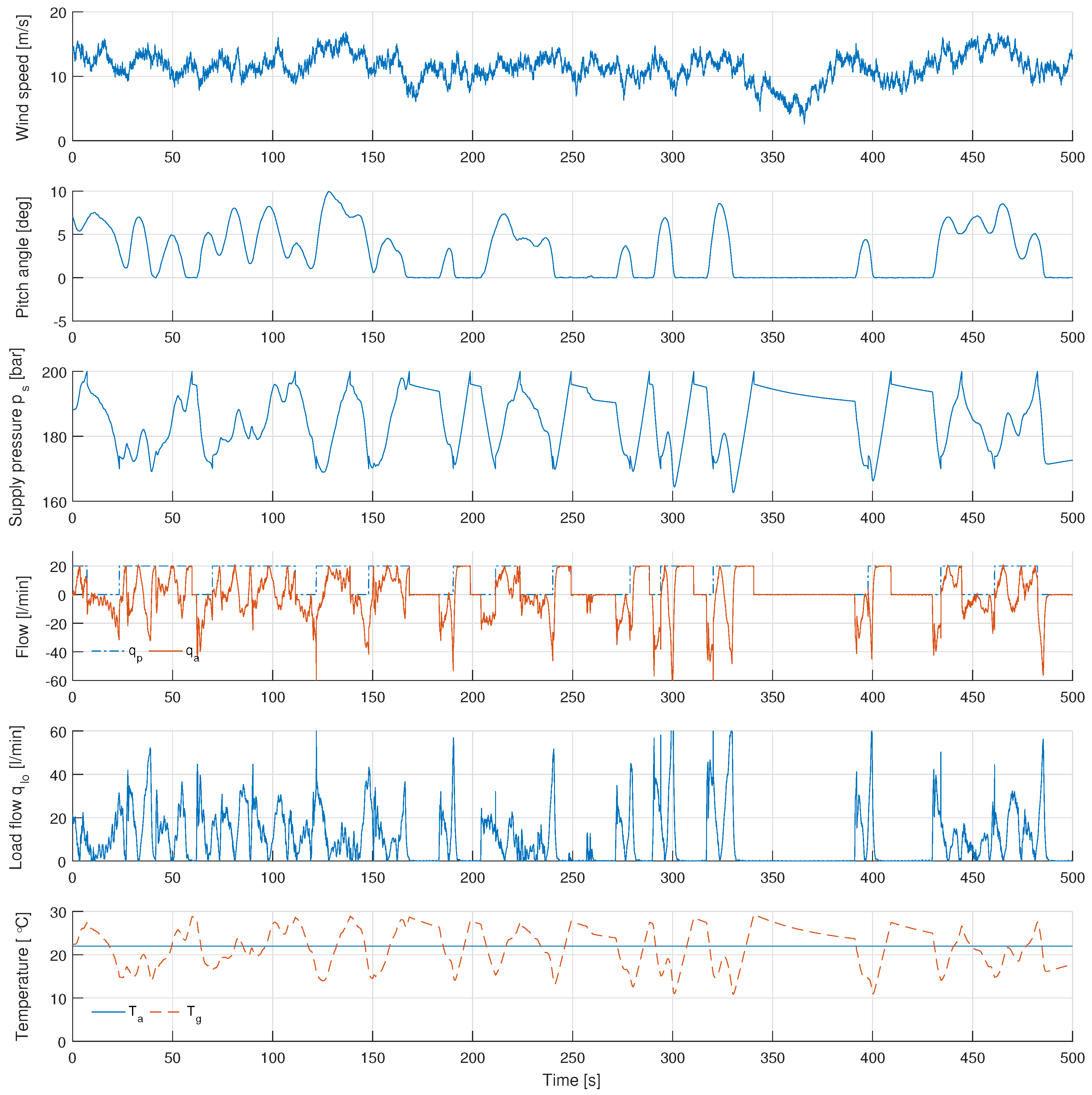
Figure 2 shows the main states of the accumulator simulated under nominal operating condition where the pre-charge pressure is set to 100 bar. The external leakage flow is set to zero. The wind speed is seen to fluctuate around the rated value, and the pitch angle changes accordingly. As expected, the supply pressure cycles between 170 and 200 bar, and the pump is seen to activate and deactivate when these limits are reached. The load flow, $q_{lo}$, increases when the pitch angle slope increases. The gas temperature is seen to increase when the accumulator is charging and vice versa for discharging. It is noted that the presented accumulator model also holds for bladder-type accumulators if the thermal time constant in Equation (5) is adapted accordingly.

3.2. Fault Analysis

The fault analysis is conducted using a linearized approximation of the nonlinear accumulator model. The linearization is evaluated at the operating point ${\overline{x}}_0=(p_{s0},{\dot{V}}_{g0},T_{g0})$. The Δ denotes the perturbation around this operating point. The linearized equation of state is given in Equation (6).

$$\begin{array}{c}\hfill \Delta p_s=K_{pv}\Delta V_g+K_{pt}\Delta T_g\end{array}$$

(6)

where $K_{pv}={\left.\frac{\partial p_s}{\partial V_g}\right|}_{{\overline{x}}_0}$ and $K_{pt}={\left.\frac{\partial p_s}{\partial T_g}\right|}_{{\overline{x}}_0}$.

Equation (7) presents the linearized energy balance for the gas.

$$\begin{array}{c}\hfill \Delta {\dot{T}}_g=K_{\dot{t}v}\Delta V_g+K_{\dot{t}t}\Delta T_g+K_{\dot{t}\dot{v}}\Delta {\dot{V}}_g\end{array}$$

(7)

where $K_{\dot{t}v}={\left.\frac{\partial {\dot{T}}_g}{\partial V_g}\right|}_{{\overline{x}}_0}$, $K_{\dot{t}t}={\left.\frac{\partial {\dot{T}}_g}{\partial T_g}\right|}_{{\overline{x}}_0}$ and $K_{\dot{t}\dot{v}}={\left.\frac{\partial {\dot{T}}_g}{\partial {\dot{V}}_g}\right|}_{{\overline{x}}_0}$. The transfer function between the flow difference $\Delta Q=q_p-q_{lo}$ and supply pressure $p_s$ is found by taking the Laplace transform of Equations (6) and (7) and using the flow continuity given in Equation (1). The transfer function is given below in Equation (8). Note that coefficients $K_1$, $K_2$ and $K_3$ are all positive in the entire operating range.

$$\begin{array}{c}\hfill \frac{\Delta P_s\left(s\right)}{\Delta Q\left(s\right)}=\frac{K_{1}s+K_2}{s^2+\left(k_{le}{K}_1+K_3\right)s+k_{le}{K}_2}\end{array}$$

(8)

where $K_1=-K_{\dot{t}\dot{v}}{K}_{pt}-K_{pv}$, $K_2=K_{pv}{K}_{\dot{t}t}-K_{pt}{K}_{\dot{t}v}$ and $K_3=-K_{\dot{t}t}$. Positive values of $\Delta Q$ correspond to charging the accumulator with fluid and vice versa for negative values. In the case of zero external leakage, i.e., $k_{le}=0$, the transfer function reduces to a Type 1 system with real poles at zero and $-K_3$ and a zero at $-\frac{K_2}{K_1}$.

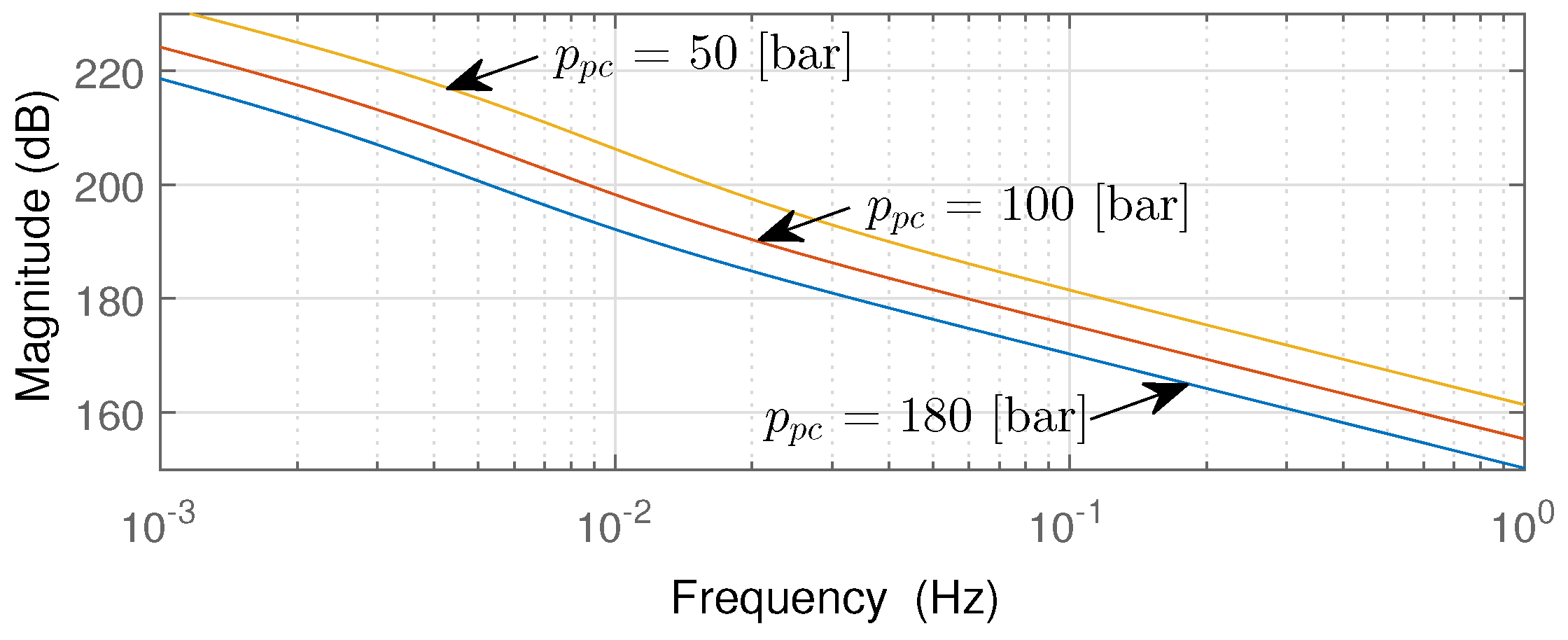
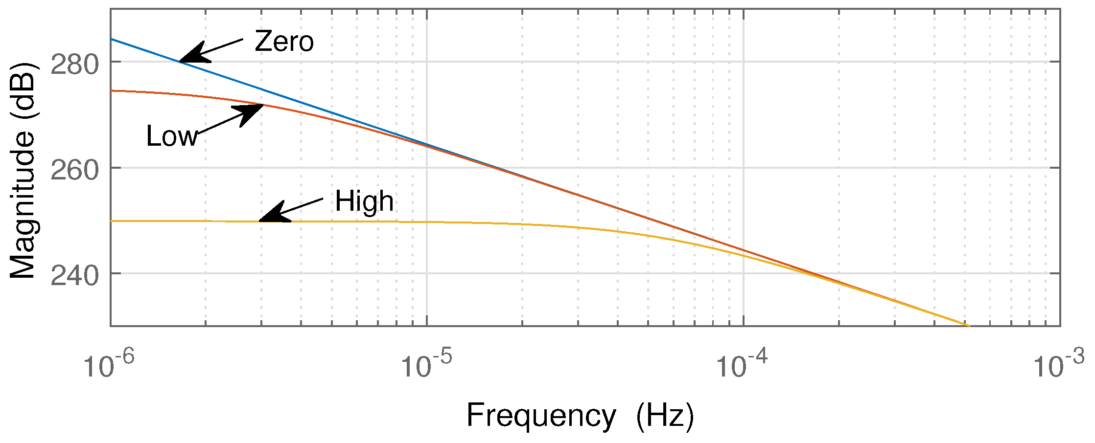
The effect of gas leakage on the supply pressure is evaluated from the frequency response at different pre-charge pressures presented in Figure 3. The transfer function is linearized at the operating point ${\overline{x}}_0=(p_{s0},{\dot{V}}_{g0},T_{g0})=\left(185\mathrm{bar},10\mathrm{L}/\min ,22{}^{\circ }\mathrm{C}\right)$. The operating point pressure, $p_{s0}$, is chosen as the midpoint between the two limits of the pressure controller. The gas volume change is chosen positive, i.e., when the fluid discharge from the accumulator, and the value is chosen as a mean from simulations. The gas temperature is set equal to the nominal temperature. The effect of the pre-charge pressure is seen to be similar to a change in gain between flow and pressure. The gain increases when the pre-charge pressure decreases. This confirms that the variations in load flow is amplified in the supply pressure when the gas leakage occurs.

The effect of external fluid leakage is seen in Figure 4. As expected, external fluid leakage decreases the low frequency gain as the system changes from Type 1 to 0. The supply pressure signal is therefore unaffected by external leakage at frequencies higher than 0.1 mHz.

4. Fault Detection Method

In this section, the fault detection method will be described, followed by a study on how the supply pressure signal obtained from simulation is affected by gas leakage. Additionally, the robustness to non-nominal operating conditions and multi-fault scenarios will be investigated.

The Multiresolution Signal Decomposition (MSD) method is used in this study to extract features of the measured signal to indicate faulty behaviour. The MSD method is based on oscillatory time limited waveforms called wavelets. Only a brief description in relation to the application is presented in this paper. A more thorough description of wavelets and MSD is found in [28,29,30]. Several advantages arise from using wavelets contrary to the similar more widely-used Fourier analysis. While Fourier analysis on its own is limited to the frequency domain, wavelets enable simultaneous time and frequency domain analysis of signals. In addition, signal decomposition using wavelets adds the flexibility of choosing different waveforms, known as a mother wavelet, rather than just the sine wave. This is important, as this allows for better filtration of the wanted characteristics of a measured signal [30].

The $l\mathrm{th}$-level discrete decomposition of a time series $g\left(t\right)$ is given below.

$$\begin{array}{c}\hfill g\left(t\right)=\sum _k{a}_l\left(k\right)2^{1/2}\varphi \left(2t-k\right)+\sum _{j=1}^l\sum _k{d}_j\left(k\right)2^{l+1-j}\psi \left(2^{l+1-j}t-k\right)\end{array}$$

(9)

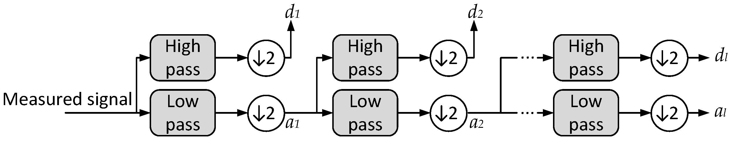
where ψ denotes the mother wavelet and is closely related to the scaling function ϕ. $d_j\left(k\right)$ is known as the $j\mathrm{th}$-level detail coefficients, and $a_l\left(k\right)$ is known as the approximation coefficients at the $l\mathrm{th}$-level. k denotes the time translation. In this study, the detail coefficients are used for fault detection, and the methods for determining the coefficients are presented in Figure 5. The measured signal is decomposed using a series of Quadrature Mirror Filters (QMF) creating a high pass and low pass version of the signal. These filters are constructed based on the mother wavelet and scaling function. The detail coefficient, $d_j$, is the output of the high pass filter, and the approximation coefficient, $a_j$, is the output of the low pass filter. At each level, the signal is downsampled by a factor of two. The detail coefficients at each level describe the original signal in frequency ranges depending on the sampling frequency, $f_s$, according to Equation (10). It is noted that some overlapping in frequency occurs between each level [29]. In this paper, the sample frequency for both simulated and measured signals is $f_s=200$ Hz.

$$\begin{array}{c}\hfill \left(f_{d_j\mathrm{Low}},f_{d_j\mathrm{High}}\right)=\left(\frac{f_s}{4j},\frac{f_s}{2j}\right)\end{array}$$

(10)

The decomposition of the pressure signal is implemented using the MATLAB wavelet toolbox (Version 4.16) [31]. In previous studies considering fault detection in fluid power systems, the eighth order Daubechies mother wavelet has proven to yield good results [14,15]. In this study, the fifth order Daubechies mother wavelet has shown to be most sensitive to the considered faults and is therefore used throughout this paper.

Simulation Results

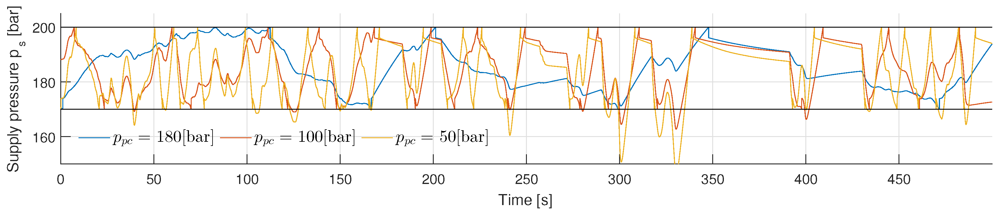
Recall that gas leakage corresponds to a change in the accumulator pre-charge pressure. Figure 6 shows 500 s of the simulated supply pressure signal for three levels of pre-charge pressure where the wind turbine is operated in nominal conditions. The supply pressure is seen to vary between the 170 and 200 bar limits of the pressure controller with occasional drops below the lower limit. The drops are more frequent for the lowest pre-charge pressure and concur with the diminished ability to compensate for the load flow magnitude during high pitch activity.

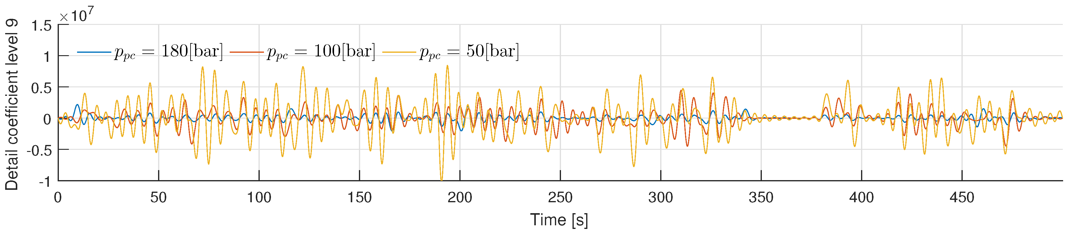
As was explained above, the detail coefficients describe features of the original signal in each frequency range. For example, take the detail coefficient Level 9, which covers the frequency band 0.39–0.78 Hz. This detail coefficient is seen in Figure 7 for the supply pressure signals shown in Figure 6. From the linear model analysis, it was found that a gas leakage fault would amplify load flow variations in the supply pressure. This is clearly the case, as the detail coefficients in Figure 7 show a significant increase in amplitude with a decrease in pre-charge pressure. Since the detail coefficient varies with time, the RMS of the coefficient is used as a comparative measure for detecting a fault. A similar approach is used by Goharrizi and Sepehri [15]. It is noted that the window size for which the RMS is calculated must be chosen large enough to capture the wanted features of the signal [32]. On the other hand, choosing a small window size promotes fast detection. Here, a window size of 500 s has been found to be the best compromise between detection time and robustness. The windows size is justified by gas leakage normally being a fault that develops over a significantly larger time scale. As discussed in the selection of operating conditions, the wind turbine must be in continues operation in the period of detection. The window of data is discarded if the turbine shuts down, e.g., due to wind speeds above cut-off. Detection is then permitted when the turbine restarts.

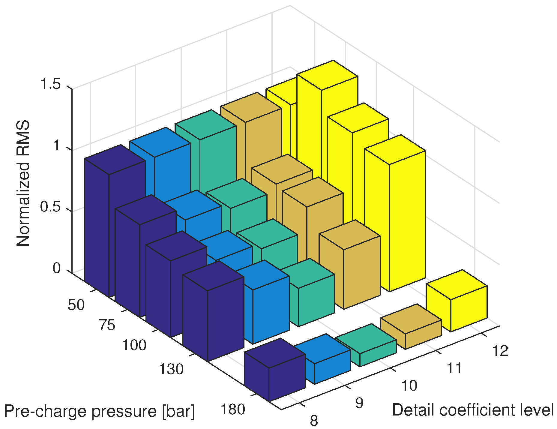
The RMS values of the detail coefficient Levels 8–12 for five levels of pre-charge pressures are shown in Figure 8. The RMS values are normalized to allow for comparison between the detail levels. The RMS values at Levels 8–11 are generally seen to increase with decreasing pre-charge pressure. The change in RMS between the pre-charge pressures indicates how sensitive the detail coefficients are to gas leakage. The change in percent is given in

Table 3. Change in RMS values of the detail coefficient decomposition Levels 8–12 for nominal operating conditions. Change in percent is given with respect to the larger RMS value. Largest change in percent is marked in bold.

Pre-Charge Pressure (bar)	180–130	130–100	100–75	75–50	Frequency Range (Hz)
RMS detail Level 8	111%	8%	21%	32%	0.78–1.56
RMS detail Level 9	164%	10%	34%	53%	0.39–0.78
RMS detail Level 10	192%	40%	38%	64%	0.20–0.39
RMS detail Level 11	283%	31%	4%	51%	0.10–0.20
RMS detail Level 12	294%	6%	17%	−22%	0.05-0.10

, and larger percent-values represent more sensitivity to the fault. The highest values are marked in bold. From Table 3, it is seen that the RMS of Level 10 shows the largest percent-values for pre-charge pressures below 130 bar. The detail Level 12 is the most sensitive above 130 bar. Generally, the sensitivity to gas leakage above 130 bar is seen to increase when the frequencies contained in the detail coefficient decrease. This is caused by the low frequency load and unload cycles seen in Figure 6. As the pre-charge pressure lowers, these cycles become more frequent. However, the cycle frequency is also very dependent on the load flow and external leakage. It is therefore not regarded as a robust indicator of gas leakage. Indications are therefore that the RMS Level 10 is most sensitive to gas leakage based on the results from nominal operating condition. Robustness to other operating conditions is, however, important for the method to be usable. Figure 9 shows the RMS of detail Level 10 for the different operating conditions as described in Section 2. The grey bars represent the mean values of several simulated conditions and the black error bars indicate the entire range of values. If the range of values overlap between the pre-charge pressures, the method is not robust to the considered operating conditions because the gas leakage levels cannot be isolated. Figure 9a shows the effect of the mean wind speed and turbulence intensity. The mean wind speed is either 11.4, 13 or 19 m/s. Both turbulent intensity Classes A and C are simulated for all wind speeds. The RMS value is seen to be less robust at lower pre-charge pressures, but no overlapping values occur.

The effect of ambient temperatures $-20,0,22,60{}^{\circ }\mathrm{C}$ is shown in Figure 9b. A large range of values is seen at each pre-charge pressure. It it seen that changes in ambient temperature present the largest disturbance compared to the other operating conditions. However, no values are overlapping.

Figure 9c shows the nominal operating condition when gas leakage and external fluid leakage faults are introduced simultaneously. The considered external fluid leakage levels are zero, low and high. The effect of external fluid leakage fault is seen to be insignificant. This is expected, as the frequency response of the accumulator was shown to be unaffected in the detail coefficient Level 10 frequency range.

In Figure 9d, all combinations of operating conditions are shown. Note that all combinations entail 216 individual simulations. The RMS values overlap for the three levels of pre-charge pressures, which shows that the method is not robust for all variations in the considered range of operating conditions.

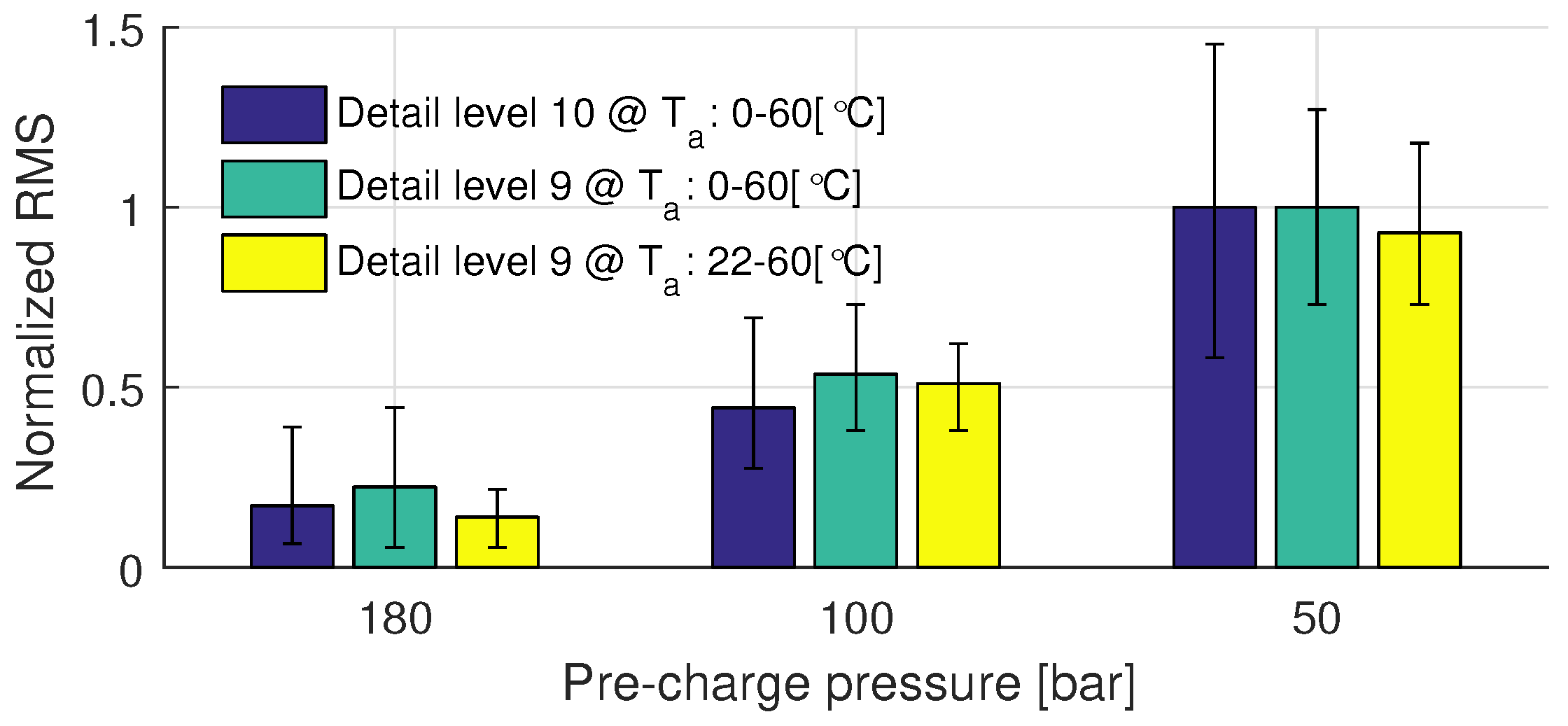
Figure 9b indicates that the ambient temperature is the most significant influence on the RMS value. The result of reducing the temperature range can be seen in Figure 10. The RMS values are normalized to enable comparison between the two decomposition levels. At a reduced temperature range of 0–60 ${}^{\circ }\mathrm{C}$, the RMS of detail Level 9 was found to be the most robust of all considered decomposition levels. In comparison to Level 10, the difference between 100 and 50 bar can be isolated for all conditions. Further reduction of the temperature range to 22–60 ${}^{\circ }\mathrm{C}$ enables isolation of all three pressure levels. The full temperature range considered in this study follows the specifications from the IEC 61400-1 design standard. However, in most cases, the temperature in the hub, which is the normal location of the accumulator, is higher than the ambient temperature of the turbine. This is mainly caused by efficiency losses in the power train and the frequency converter. The reduced temperature range needed for the fault detection to be robust is therefore not considered as a major drawback.

5. Experimental Verification

In this section, the experimental setup will be described, and the results will be presented. The setup and corresponding diagram are seen in Figure 11. The setup is constructed to emulate the conditions for the accumulator in the pitch system of a wind turbine. This is done by controlling the pump pressure and load flow according to the simulation. The fault detection method can therefore be tested using the actual dynamics of an accumulator without the need for expensive tests in a wind turbine. Additionally, the setup allows for testing in a multi-fault environment by considering simultaneous gas and external fluid leakage. Details about the controller, components and sensors used in the setup are given in

Table 4. Main data for the sensors and components used in the experimental setup.

Name	Item	Specifications
Hydroll piston accumulator	A1	Capacity: 6 (L)
Danfoss MBS 3050	T1-T3	Signal: analogue 4–20 (mA)
pressure transducer		Range: 0–350 (bar)
		Full scale accuracy: <1%
		Rise time: <4 (ms)
Parker SCQ-060	T4-T5	Signal: analogue ±3 (V)
flow meter		Range: ±60 (L/min)
		Full scale accuracy: <2%
		Rise time: <2 (ms)
VSE VSI 0.04/16	T6	Signal: digital 0–5 (V)
gear flow meter		Range: 0–2 (L/min)
		Full scale accuracy: <0.04%
Hydratech 2/2 NC poppet	V1	Opening time: 30 (ms)
cartridge valve		Closing time: <120 (ms)
		$\Delta p$: 1 (bar) @ 10 (L/min)
Bosch Rexroth 4WREE N6	V2	Small signal band width: 50 (Hz)
4/3 way proportional valve		Rated flow: 32 (L/min) @10 (bar)
Tognella adjustable	V3	Rated flow: 0–8 (L/min)
needle valve
Controller		OS: Simulink Realtime
		I/O card: NI 6221

. To emulate real load flow conditions, valve V2 is operated in closed loop governed by a proportional controller with feed forward to achieve a given flow reference. The flow sensor T4 acts as a feedback for the proportional term. The valve pressure drop measured by sensors T2 and T3 is used in conjunction with the valve characteristics for generating a feed forward dependent on the flow reference. The pump flow is controlled by switching valve V1 on or off.

The experimental setup is equipped with an accumulator having a capacity of six litres compared to 50 L of an actual system. This difference is compensated by scaling the pump and load flow such that the pressure variations of the setup are similar to those found in the pitch system. The scaling factor is determined as the ratio of the magnitude response between a 6-L and 50-L accumulator calculated from Equation (8). It is noted that the scaling factor has a negligible dependency on frequency and can be set to a fixed value of 0.12. It is noted that this value also corresponds to the volume ratio between the test and real-life accumulator. The leakage flow levels are scaled similarly to the load and pump flow.

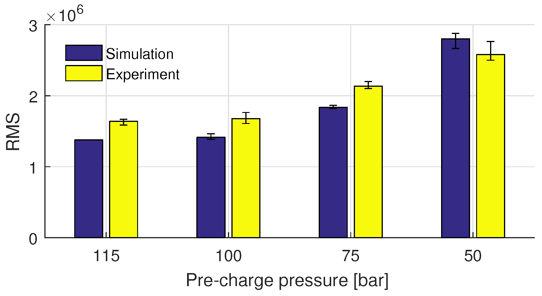
The experiments are performed using flow references from the nominal operating condition and three levels of external fluid leakage. As an example, the measured flows and supply pressure for a 20-s window are seen Figure 12. The load flow is seen to track the reference well, but due to internal leakage of valve V2, the flows below 0.5 L/min are not reached. The external leakage flow is seen to reach 0.12 L/min at 200 bar, which concurs with the scaled value of the high leakage flow level. The results of the experiments compared to simulations are shown in Figure 13. The RMS values are calculated for detail Coefficient 9 in the nominal operating condition and all three levels of external leakage flow. For statistical purposes, each experiment is performed twice, whereby the total amount of the experiments is 24. Similar to the simulation results, the experiments show an increasing tendency in RMS when the pre-charge pressure decreases. The difference in RMS of the experiments compares well to the simulations from 115 to 75 bar pre-charge. The experiment is not as sensitive to gas leakage at the lowest 50 bar pre-charge pressure; however, the value can still be isolated from the other levels. The discrepancy is subscribed mainly to internal leakage of valve V2 and the flow restriction caused by the flow meter T6. This restriction is not present in the simulated system, and it will dampen the supply pressure fluctuations. The range of values at each pre-charge pressure is very similar to the simulated results, which confirms the high robustness of the method to external fluid leakage. The variation of the RMS values indicated by the error bars is mainly caused by external leakage.

6. Discussion

The signal-based method for gas leakage detection builds on the hypothesis that naturally occurring variations in the supply pressure signal are amplified if the accumulator experiences a gas leakage. However, the pressure signal variations are dependent not only on the gas leakage fault, but also on operating conditions, as well as other faults. The detail Coefficient 9 covering the frequencies 0.39–0.79 Hz is found most robust as a fault indicator. This can be explained from a special disturbance to the pitch systems caused by the tower effect. The tower effect is a cyclic event that affects each blade of the turbine. The local wind speed changes as a blade passes by the tower, which results in an external load acting on the pitch cylinder. This external load disturbance propagates from the three blades to the supply pressure, which creates distinct variations three times per revolution (3P). At the nominal hub speed, the 3P frequency is 0.6 Hz. Therefore, the detail coefficient selected for accumulator gas leakage detection can preferably be chosen such that it covers the 3P frequency.

7. Conclusions

A signal-based gas leakage detection method was proposed for accumulators used in wind turbines. The method employed multiresolution signal decomposition based on wavelets. It was shown that the detail Coefficient 9 of the supply pressure signal was sensitive to gas leakage faults. Detail coefficient Level 9 corresponds to a frequency range of 0.39–0.78 Hz, which yielded the best results due to the inclusion of the 3P frequency of 0.6 Hz. The simulation results showed that the proposed method could detect and isolate several levels of pre-charge pressure during nominal operating condition of a wind turbine. The method also showed very robust results in a multi-fault environment where external fluid and gas leakage occurred simultaneously. From the results, it was furthermore found that low ambient temperatures considerably degraded robustness, and for all combinations of operating conditions, the method was not applicable. However, the robustness is increased as the minimum ambient temperature is increased. Changes in pre-charge pressure from 180 bar to 100 bar and to 50 bar were detectable and were isolated in an ambient temperature range of 22–60 ${}^{\circ }\mathrm{C}$. The efficacy of the method was further validated on an experimental setup, where a small-scale accumulator was operated according to the nominal conditions in a wind turbine. The experiment was also conducted in the multi-fault scenario considering simultaneous gas and external fluid leakage. The experimental results showed good correlation to the simulations and indicated that the signal-based gas leakage detection method was indeed effective and beneficial for the wind turbine industry.