A New Method of Ground Fault Location in 2 × 25 kV Railway Power Supply Systems

Abstract

Owing to the installation of autotransformers at regular intervals along the line, distance protection relays cannot be used with the aim of locating ground faults in 2 × 25 kV railway power supply systems. The reason is that the ratio between impedance and distance to the fault point is not linear in these electrification systems, unlike in 1 × 25 kV power systems. Therefore, the location of ground faults represents a complicated task in 2 × 25 kV railway power supply systems. Various methods have been used to localize the ground fault position in 2 × 25 kV systems. The method described here allows the location of a ground fault to be economically found in an accurate way in real time, using the modules of the circulating currents in different autotransformers when the ground fault occurs. This method first needs to know the subsection and the conductor (catenary or feeder) with the defect, then localizes the ground fault’s position.

1. Introduction

Currently, the most widely used electrical configuration to feed high-speed trains is the 2 × 25 kV railway power system. The use of this system, compared to the traditional 1 × 25 kV railway power system, allows the required number of traction substations erected along the line to be reduced, because it has lower losses and lower voltage drops along the line [1].

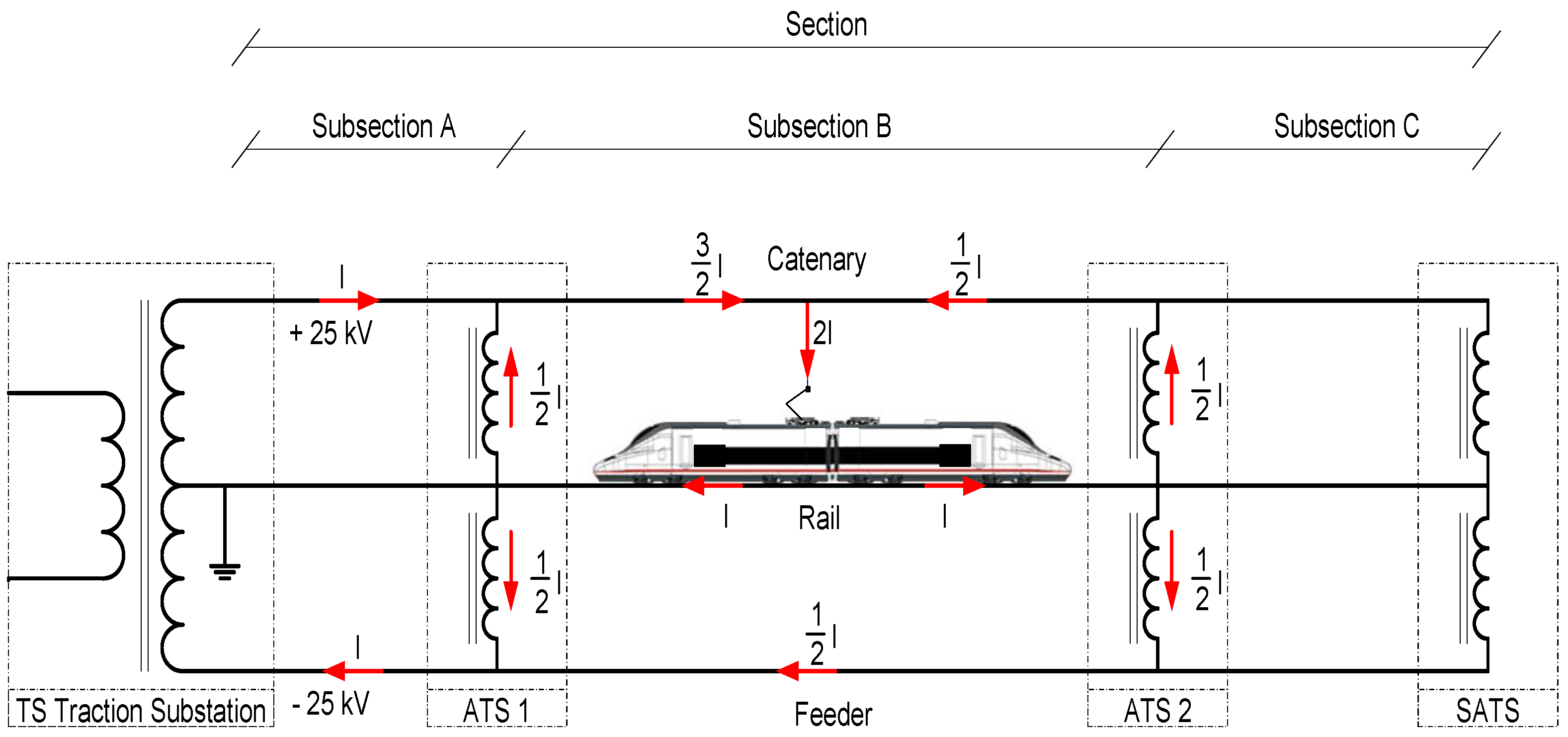
In this 2 × 25 kV system, each traction substation feeds two sections, one in each direction of the line. Each section consists of several subsections of similar length that are delimited by autotransformer power stations (ATS). These autotransformers have two terminals; one is connected to the positive conductor rated 25 kV (catenary), while the other is connected to the negative conductor, also rated 25 kV (feeder). The midpoint of its winding is connected to the rail and ground. Another autotransformer (SATS) is installed at the end of the section and is connected in the same manner as the intermediate autotransformers (Figure 1).

Electrical installations need adequate protection to ensure a reliable and safe operation [2]. This need is accentuated in the case of electric railway traction systems due to the increased number of failures caused by the sliding of the pantograph on the contact wire, which can cause its breakage. These faults cause severe economic and social problems by disrupting rail services. Therefore, it is very important to detect and locate the point where the ground fault has occurred in order to isolate the subsection at the fault, and to repair such a failure as quickly as possible [3].

In AC electrical traction systems, the most-used method for measuring the distance from a traction substation to a ground fault due its stability, reliability and simplicity, is the impedance method [4,5]. However, in 2 × 25 kV traction power systems, it is not possible to determine the distance from the traction substation to the ground faults in an acceptable manner with this method [6]. This is due to the presence of autotransformers that make the ratio impedance-distance nonlinear [7].

To be able to use this location method and to know the distance to the ground fault through the impedance seen from the traction substation, it is necessary to disconnect the autotransformers and separate the catenary from the feeder circuits when a ground fault is detected. Thus, the subsection is divided into two circuits with only one conductor and return cable, as in the case of 1 × 25 kV systems. Following this procedure, a ground fault can be located by measuring the impedance in each conductor and return cable circuits. This method is used in some 2 × 25 kV traction power systems, but it is very slow, requiring several operations of connection and disconnection of switches with waiting times between each maneuver [8,9].

Another traditional method used for fault location in railway power systems that employs auto-transformers is the AT neutral current ratio fault location method [10]. However, the capacity of the main transformer is much higher than that of the autotransformer stations. For this reason, this method can be insufficiently accurate and identifies failures in the wrong subsections. Therefore, a method of compensation using the neutral currents circulating in adjacent autotransformers to those of the faulty section was proposed in [11].

The location method using travelling waves, in addition to transmission and distribution lines, has been applied to the lines of railway traction power systems, aided by advances in the theory of wave propagation, microelectronics and data processing [4]. In this method, when a ground fault occurs, there are various types of technologies to locate ground faults according to the detection of the generated travelling wave at one end [12] or at both ends [13], and if it is performed by the wave itself or by a pulse injected into one end when such a fault occurs [14]. However, this method is difficult to implement because of its limited reliability, complex setup and high economic investments [15]. This difficulty is due to the specific characteristics of traction facilities with numerous discontinuities in the contact line and multiple loads changing position continuously [16].

This article describes a new ground fault location method that allows the position in the railway line where a ground fault has occurred to be obtained in real time, and also whether it has been in the catenary (positive conductor) or feeder (negative conductor). The method locates the position of the failure using the values of the modules of the currents in different autotransformers when a ground fault occurs, and is based on the knowledge of the subsection and the conductor where the ground fault has occurred following the method described in [17]. The method that identifies the subsection with a ground fault is summarized in Section 2. In Section 3, the distribution of currents in the autotransformers is presented for different ground fault locations by computer simulations. Section 4 describes the principles of the new method for ground fault location. In Section 5, the experimental results of tests carried out in the laboratory are introduced. Finally, Section 6 summarizes the main contributions of the paper.

2. Brief Description of Ground Fault Identification Method for 2 × 25 kV Railway Power Supply Systems

Figure 1 shows the simplified scheme of an electric section that is fed by a 2 × 25 kV power system with three subsections (A, B and C) delimited by intermediate autotransformers ATS1 and ATS2. At the end of the section, an autotransformer SATS connects the three conductors. Also, the distribution of currents in the conductors is represented when a train travels in the intermediate section B.

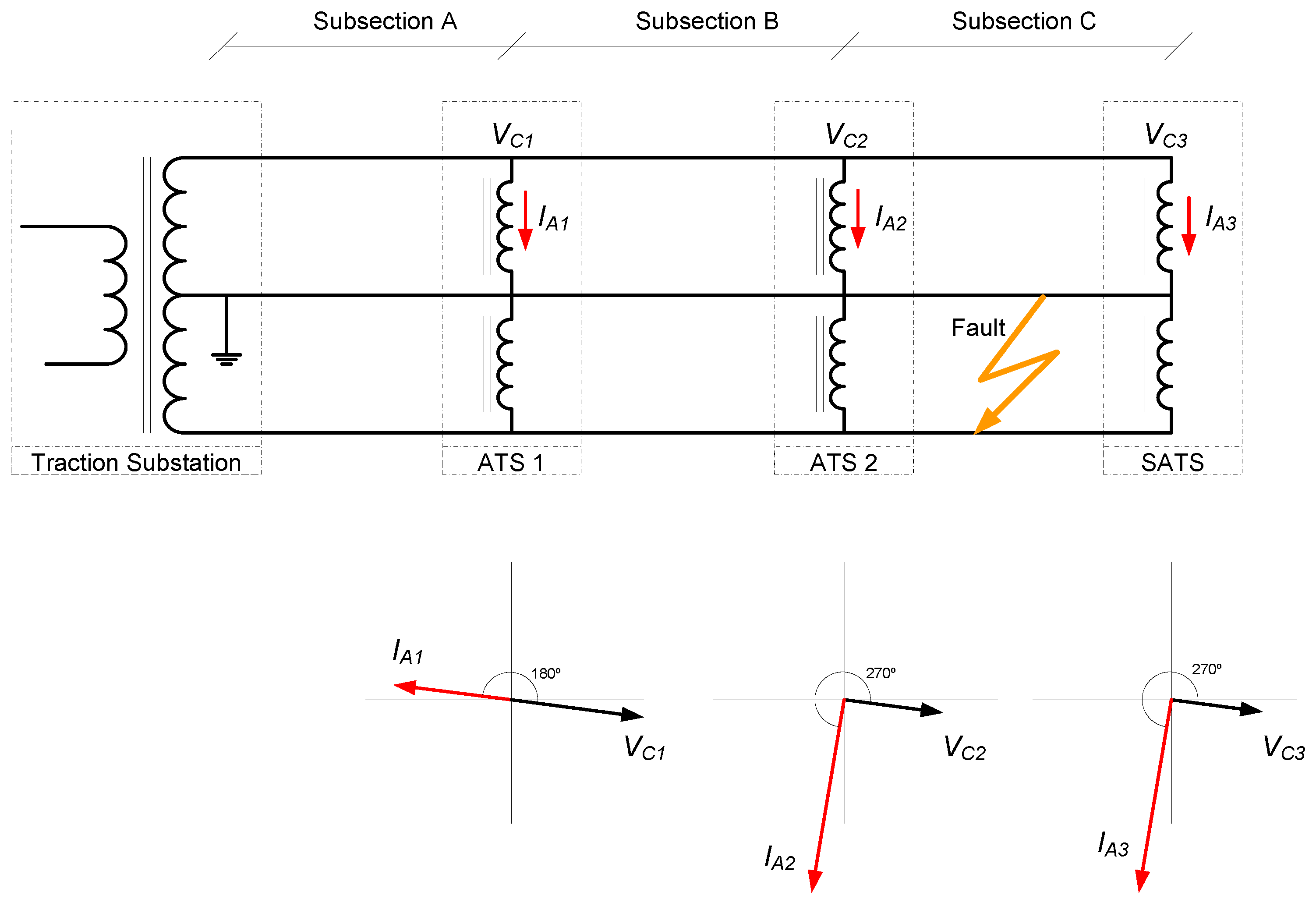
According to [17], when in a line of a 2 × 25 kV rail power system supply, a fault occurs between the catenary and rail or between the feeder and rail, there is a significant increase in the current flowing in the windings of the closest autotransformers to the position where the fault has occurred. In addition, the angles between these currents and voltages between the catenary and rail change at the location of the autotransformers.

The power factor of the high-speed trains is close to the unity, so the impedance seen from the autotransformer is mainly resistive. In a line feeding trains in normal operation without any faults, these angles are close to 180°.

But if a ground fault arises, the impedance seen from the autotransformer can be the catenary or feeder inductance. So, the angle between currents and voltages in the autotransformers closest to the fault changes increasing 90° or decreasing 90° because they are reactive currents without resistance component. There is mainly reactive power in the 2 × 25 kV supply system. In the case of ground fault between the catenary and ground, the angle between the currents and voltages in the nearest autotransformers is approximately 90°. However, if the fault occurs between the feeder and ground, the angle between the currents and voltages in the nearest autotransformers is now 270°. This last type of fault and the angles between the currents and voltages in the nearest autotransformers are shown in Figure 2.

Therefore, if the currents and voltage values, including the phase angle difference between them, are measured in the autotransformers, when a fault occurs between any conductor and the ground, it is possible to identify in which subsection the fault took place, and which conductor had such a fault.

3. Current Distribution in Autotransformers for Different Ground Fault Locations in 2 × 25 kV Rail Power Supply System

As explained before, if a ground fault takes place between the catenary and rail or between the feeder and rail in a power system fed by 2 × 25 kV, the values of the currents flowing in the windings of the closest autotransformers to the point where the fault has occurred experience a very significant increase. These values can be easily obtained by measuring the current in those windings.

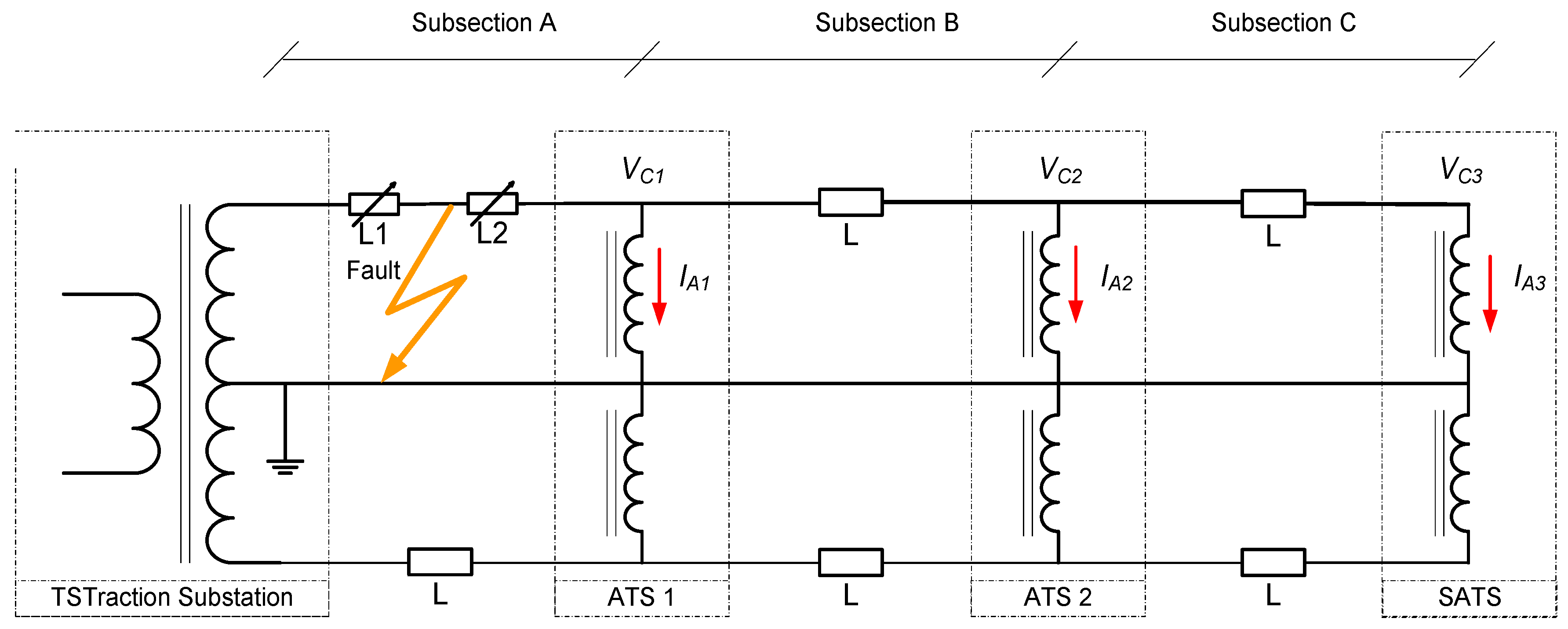
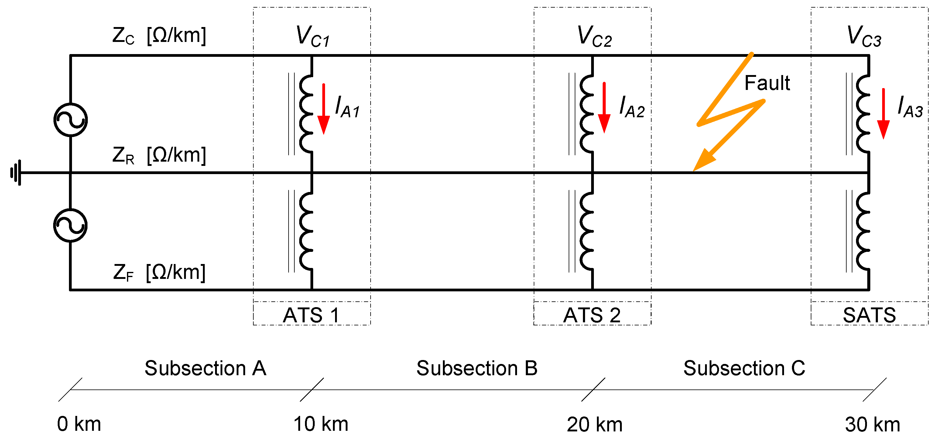
To simulate the current distributions in autotransformers when ground faults occur along all positions of a section, the circuit shown in Figure 3 was used. The modified nodal circuit analysis method [18] is applied to solve such a circuit using MATLAB (MathWorks Inc.: Natic, MA, USA).

In these simulations, a value of 27.5 kV has been given to each source of alternating current (AC) voltage. The impedance values per unit length of each conductor are listed in

Table 1. Self and mutual impedance values of railway conductors.

Conductor		Self-Impedance Ω/km
Catenary	ZC	0.1197 + j0.6224
Feeder	ZF	0.1114 + j0.7389
Rail	ZR	0.0637 + j0.5209
Conductors		Mutual Impedance Ω/km
Catenary-Feeder	ZCF	0.0480 + j0.3401
Catenary-Rail	ZCR	0.0491 + j0.3222
Feeder-Rail	ZFR	0.0488 + j0.2988

, where Z_C is the impedance value per unit length of the catenary, Z_F is the corresponding impedance of the feeder; and Z_R is the impedance of the rail that is grounded. Likewise, the values of the mutual impedances per unit length between the catenary, feeder and rail are also shown in Table 1.

The values of the impedance parameters of the transformer of the substation and of the autotransformers used in the simulation are shown in

Table 2. Transformers and autotransformers ratings used in the simulation.

Main Transformer
Voltage ratio	400/2 × 27.5	kV
Rated power	60	MVA
Short-circuit voltage	10	%
Autotransformers
Voltage ratio	55/27.5	kV
Rated power	15	MVA
Short-circuit voltage	1	%

.

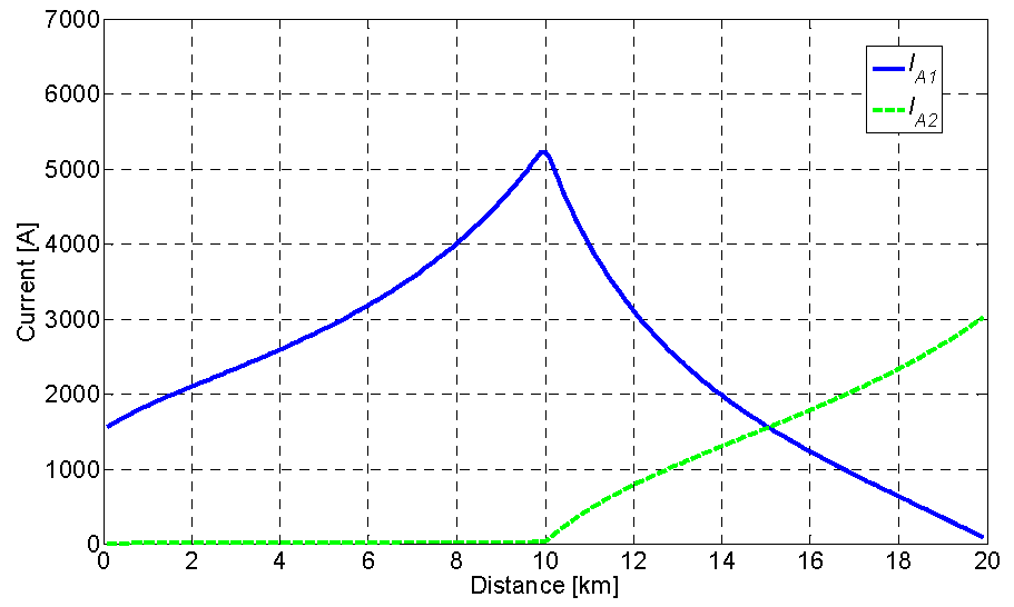
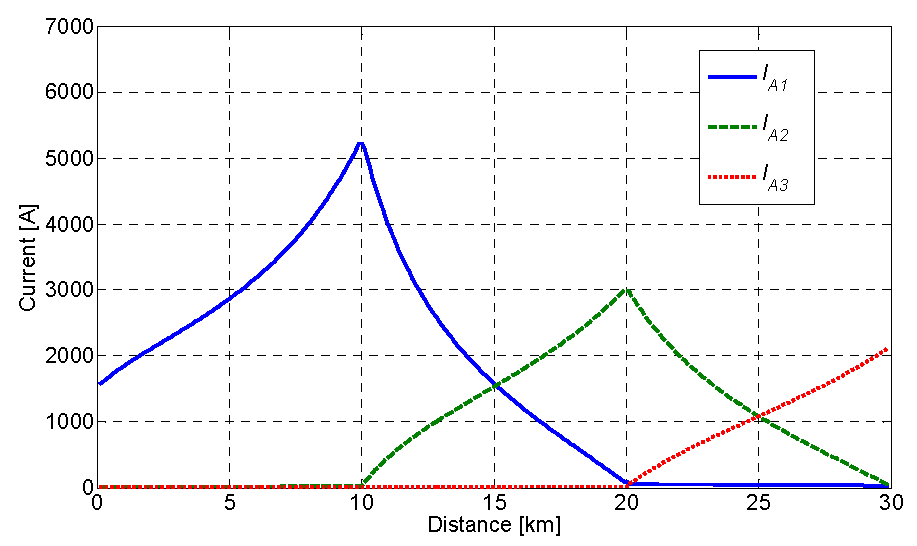
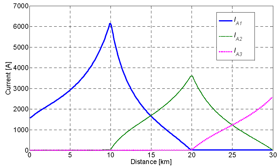
This circuit has been resolved making faults between the catenary and feeder conductors and rail in all positions of the three subsections A, B and C that compose the 30 km section. Thus, different values of the currents in the autotransformers have been obtained with ground faults at all points of the section in both cases: when the fault is between the catenary and rail and when it is between the feeder and rail. The results obtained are represented in Figure 4 and Figure 5. Figure 4 shows the values of the currents I_A1, I_A2 and I_A3 for catenary-rail faults; and Figure 5 shows the values of the currents I_A1, I_A2 and I_A3 for feeder-rail faults.

As shown in Figure 4 and Figure 5, the module of the current in each autotransformer has its highest value when the fault occurs very close to the corresponding autotransformer. It is also remarkable that the current of one autotransformer is approximately equal to that of the adjacent autotransformer at the midpoint of the section delimited by these two autotransformers. This feature is observed when the fault takes place between the catenary and rail, and also between the feeder and rail.

4. New Method for Ground Fault Location in 2 × 25 kV Traction Power Systems

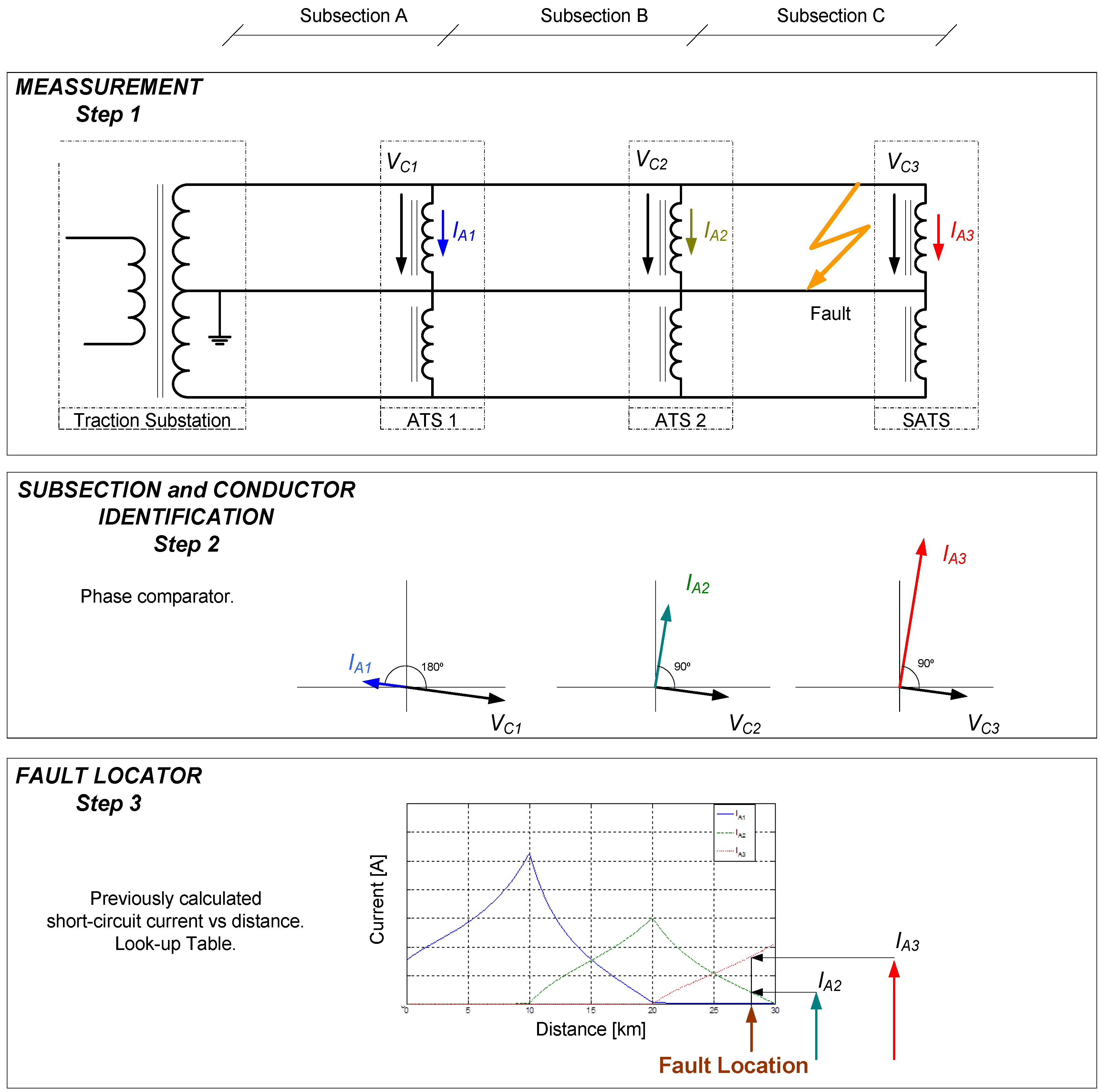
This new method for ground fault location in 2 × 25 kV power systems is divided into three different stages (Figure 6).

4.1. Measurement

In the first stage, the voltages and the currents in the different autotransformers should be measured, as well as the phase angle between them (V_C1, I_A1; V_C2, I_A2; V_C3, I_A3).

In the case of a ground fault, the current in some of the autotransformers would exceed a prefixed threshold, and the location system should be activated.

4.2. Subsection and Conductor Identification

Afterwards, the subsection between autotransformers and the positive or negative conductor where the fault has occurred are identified by analysing the phase angle between the voltages and currents in the autotransformers, as was summarised in Section 2. The completed method is described in [17].

4.3. Fault Locator

Finally, the fault locator is based on the previous calculation of the currents in the autotransformer for a ground fault along all the positions of a section, as per Section 3. The calculations should be performed specifically taking into consideration the precise data of the power system. The values of the fault current should be stored as look-up tables.

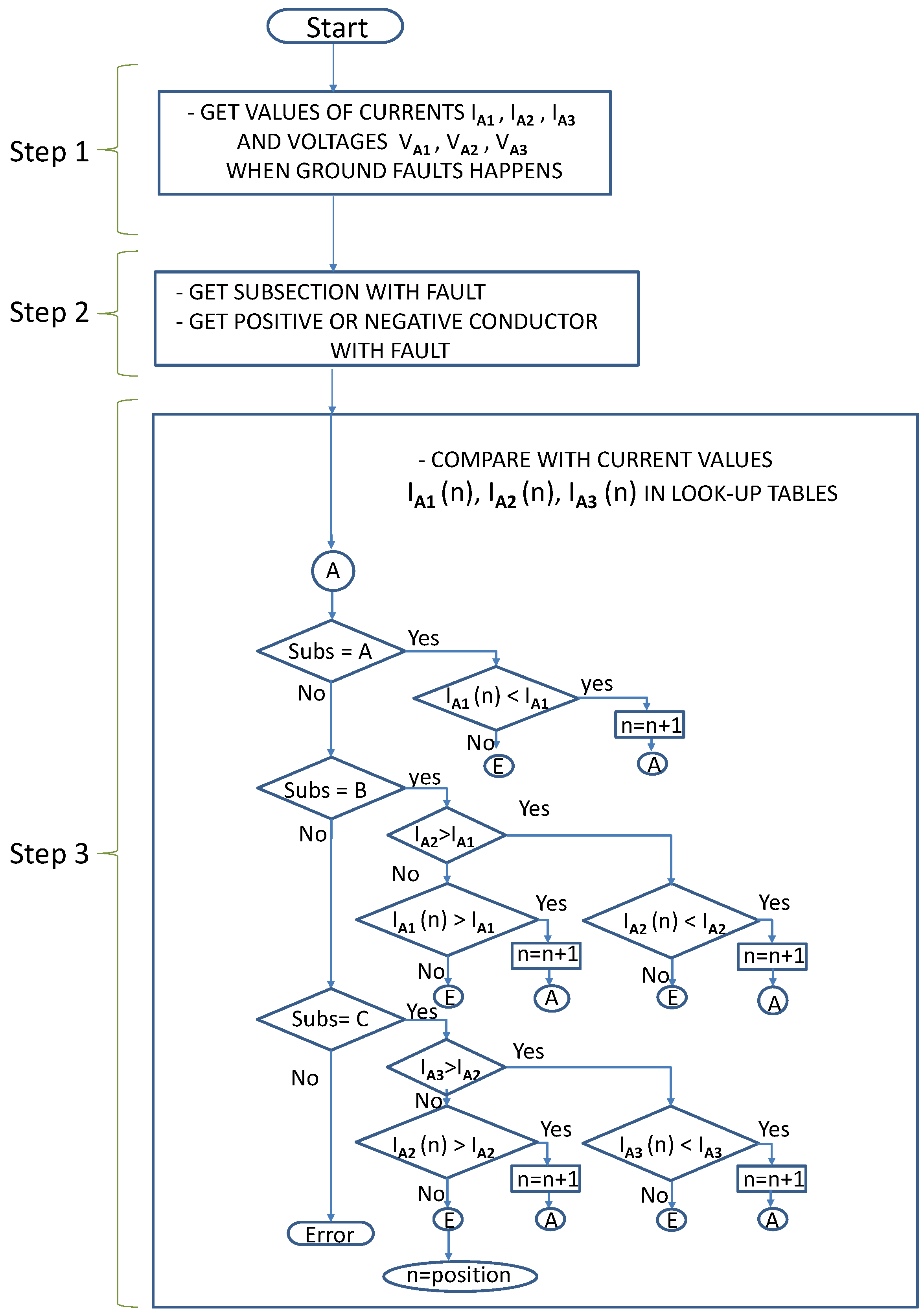
The fault location is performed by a comparison of the current measured in the two adjacent autotransformers to the pre-calculated value storage in the look-up tables. In this way, the location of the fault can be found. A flowchart of the ground fault location method is presented in Figure 7.

This method could be easily implemented in 2 × 25 kV power systems, as the voltages and currents in the autotransformers are recorded by the protection relays installed in the autotransformers, and this information is normally sent to the Supervisory Control and Data Acquisition System “SCADA”.

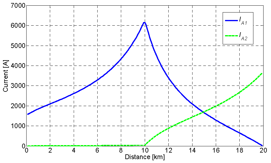
4.4. Fault Location for Sections with n Subsections

This method is also valid for any section that has at least two subsections, since the pattern that follows the values of the modules of the currents in such cases is totally similar to that in sections with three subsections.

Figure 8 and Figure 9 show the values of the current modulus as a function of the distance to the fault in a section with two subsections, both for catenary and feeder faults.

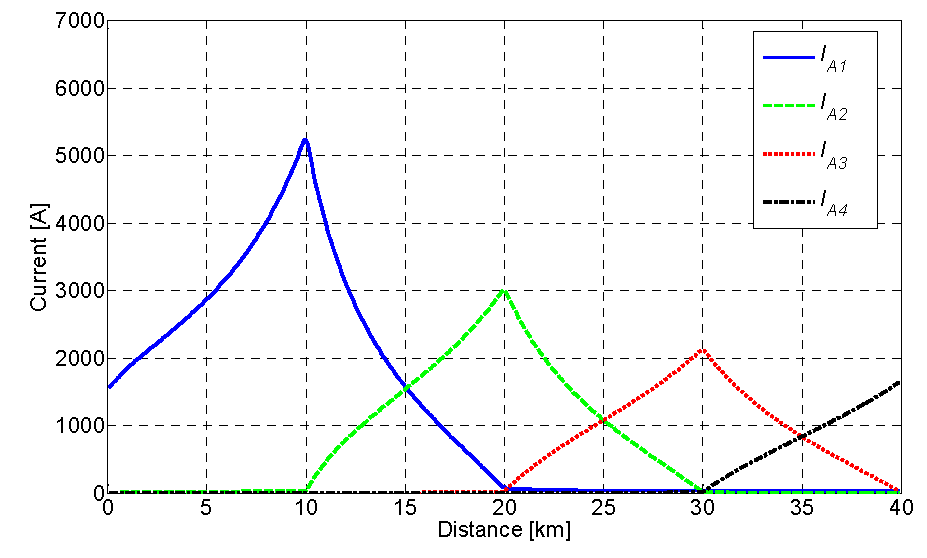
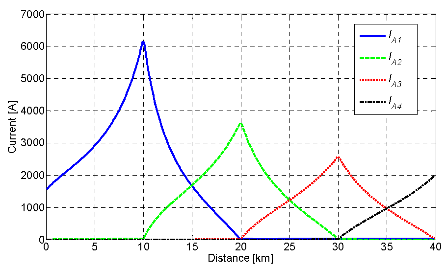
Furthermore in Figure 10 and Figure 11, the values of the current modulus are represented as a function of the distance to the ground fault in a section with four subsections for both catenary and feeder faults.

From all the results illustrated in previous figures it can be concluded that this ground fault location process is applicable to any section with two or more subsections.

5. Experimental Tests

In addition to the computer simulations, numerous tests have been performed in the laboratory to obtain the necessary tables in order to store in memory the currents of the autotransformers used in the circuit represented in Figure 12 when several ground faults are performed.

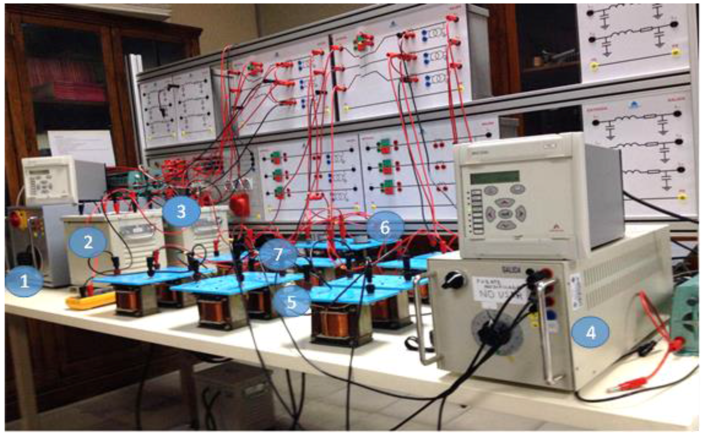
The experimental setup used in the laboratory is shown in Figure 13. It simulates the circuit of Figure 12. In this experimental setup, the traction substation was implemented using a power source (1) and the traction transformer was made using two transformers (2) and (3) providing 25 V AC each (see Figure 13).

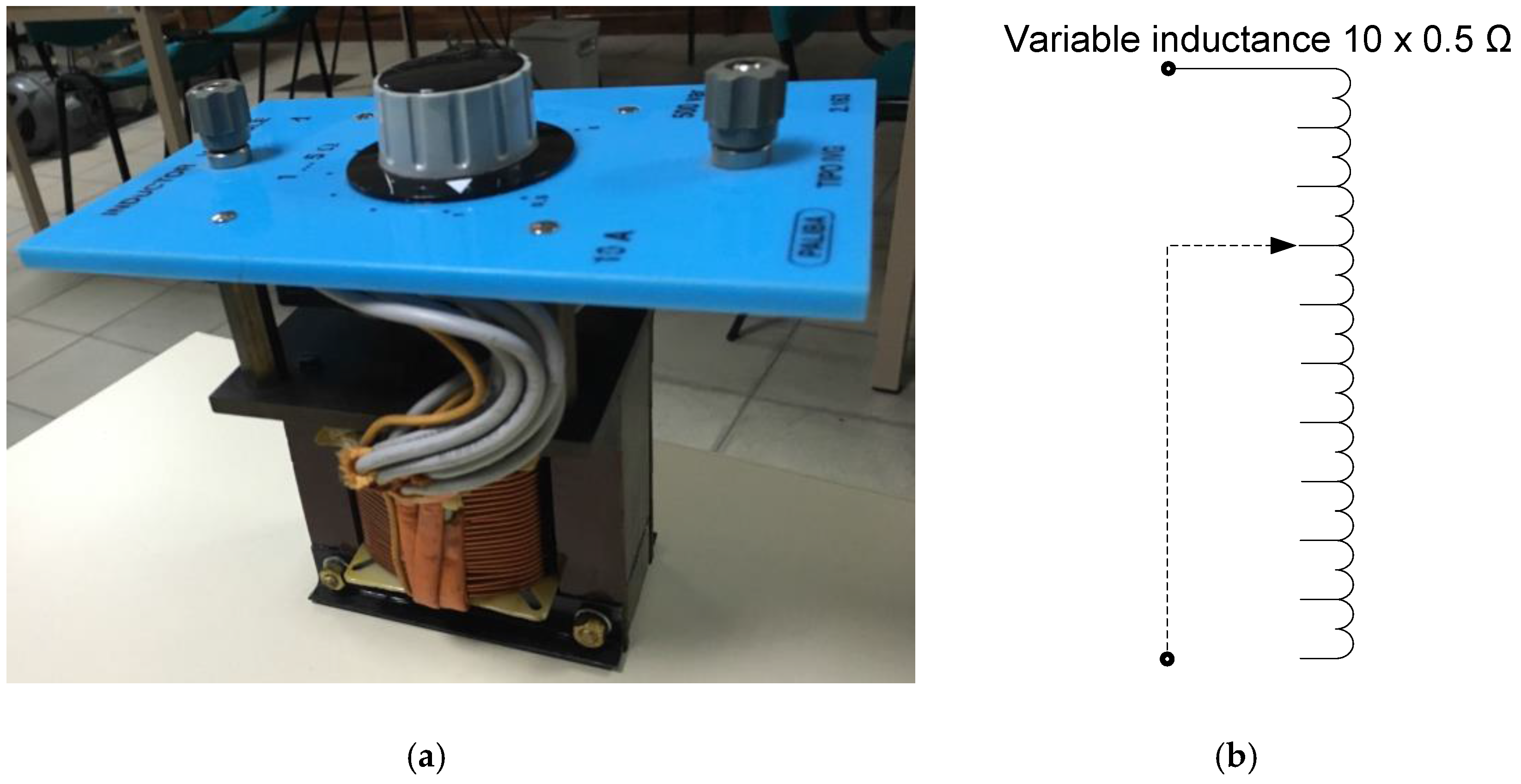
The section is divided into three subsections by autotransformers ATS1, ATS2 and SATS (4). The distributed impedances of the catenary and feeder were simulated using inductive impedances L (5). Moreover, the rail impedance was considered negligible and no impedance was installed. To simulate faults (7) along different points of each subsection, variable inductors L1 and L2 (6), were used. Such inductors can be observed in detail in Figure 14.

The values of the experimental setup impedances per unit length of the catenary, feeder and rail are shown in

Table 3. Experimental setup impedance values of railway conductors.

Conductor		Self-Impedance Ω/km
Catenary	ZC	0.10 + j1.00
Feeder	ZF	0.10 + j1.00
Rail	ZR	0

. No mutual impedances have been taken in consideration

Additional information about the transformer and autotransformers used in the experimental setup is shown in

Table 4. Experimental setup transformers and autotransformers ratings.

Main Transformer
Voltage ratio	400/2 × 25 kV	V
Rated power	1600	VA
Short-circuit voltage	5.38	%
Autotransformers
Voltage ratio	50/25	V
Rated power	300	VA
Short-circuit voltage	2.17	%

.

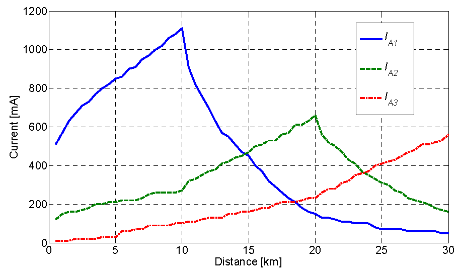
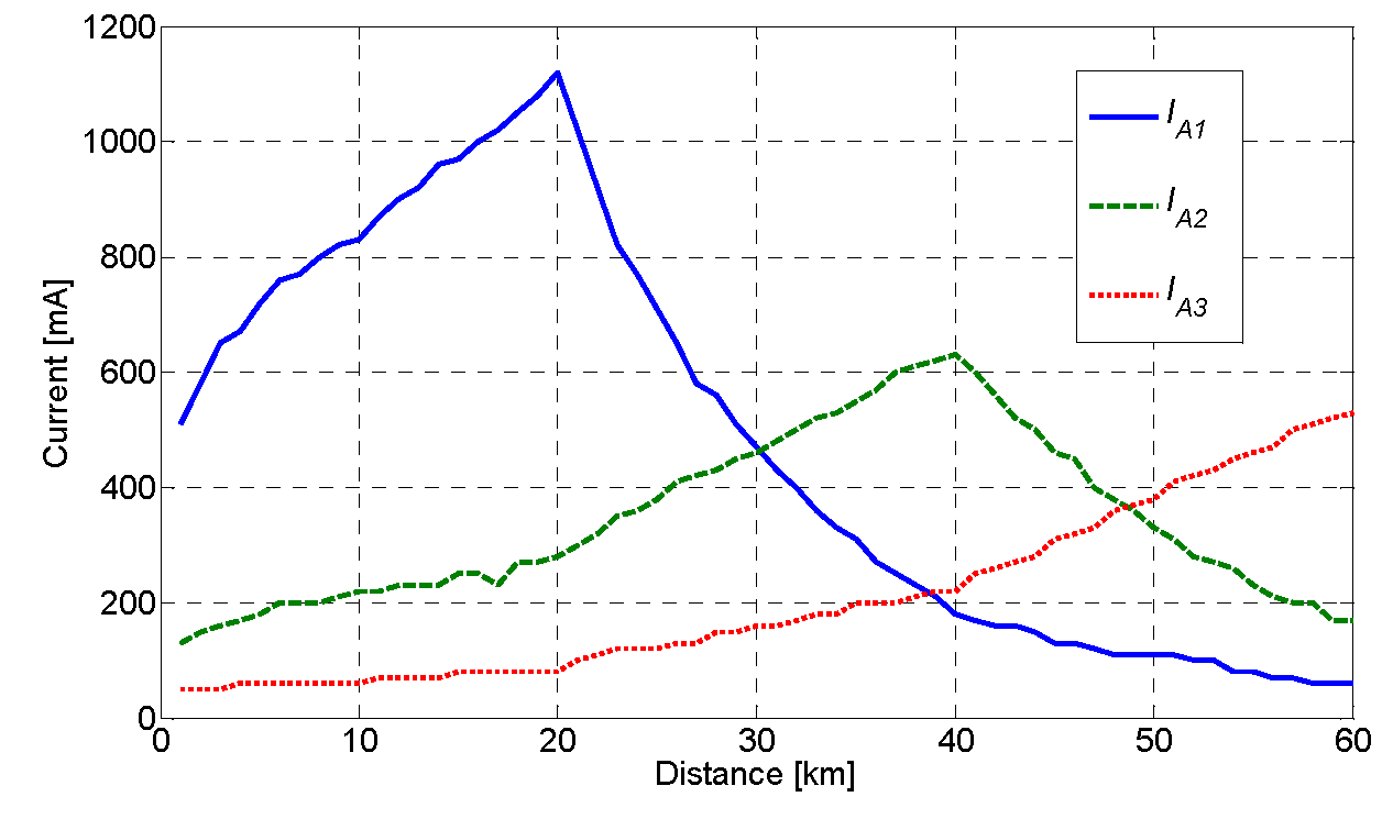
With this setup, the currents I_A1, I_A2, and I_A3 were measured. These currents were flowing in the three autotransformers used when a fault was executed between the catenary and rail. These faults were made along the section that simulated a length of 30 km with three subsections of 10 km, performing measurements every 0.5 km. Figure 15 shows the evolution of these currents depending on the position where the fault was developed for a catenary-ground fault.

Also in this facility, the currents flowing in the three autotransformers (I_A1, I_A2 and I_A3) were measured when a fault was made between the feeder and rail every 0.5 km along the section. The results are shown in Figure 16.

As it is observed, in case of ground fault, the current distributions obtained through experimental results (Figure 15 and Figure 16) are similar to those obtained through computer simulations (Figure 4 and Figure 5). Therefore the simulation model is validated, as well as the location method.

6. Conclusions

We have described a new method of ground fault location for 2 × 25 kV traction power systems based on the measurement of the currents and voltages in the autotransformers along a section.

The subsection and the positive or negative conductors where the ground fault takes place are determined by analyzing the phase angle between the voltages and the currents in the autotransformers at both ends of the subsection.

The fault location is performed by a control device, in which the values of the autotransformers currents, in the case of a ground fault along the section, have been previously recorded in its memory as look-up tables. This control device receives the readings from the autotransformers protection relays. By comparing the measured currents in the autotransformers to the previously recorded values, the fault position can be determined.

This method is also economical, as the voltage and current measurement transformers and protection relays are already installed in the autotransformer substations. The new location method could be implemented in the Supervisory Control and Data Acquisition System “SCADA” of 2 × 25 kV power systems, in which the information from autotransformer protection relays is normally available. This method has been tested by computer simulations and experimental laboratory tests, both obtaining suitable results.