Article

The Deployment of Low Carbon Technologies in Energy Intensive Industries: A Macroeconomic Analysis for Europe, China and India

1
Wegener Center for Climate and Global Change, University of Graz, 8010 Graz, Austria
2
Department of Economics, University of Graz, 8010 Graz, Austria
3
International Institute for Applied Systems Analysis, 2361 Laxenburg, Austria
4
Andlinger Center for Energy and the Environment, Princeton University, Princeton, NJ 08540, USA
5
Woodrow Wilson School of Public and International Affairs, Princeton University, Princeton, NJ 08540, USA
*
Author to whom correspondence should be addressed.
Energies 2017, 10(3), 360; https://doi.org/10.3390/en10030360
Submission received: 30 September 2016 / Revised: 9 February 2017 / Accepted: 2 March 2017 / Published: 14 March 2017
(This article belongs to the Special Issue Low Carbon Economy)

Abstract

:
Industrial processes currently contribute 40% to global CO2 emissions and therefore substantial increases in industrial energy efficiency are required for reaching the 2 °C target. We assess the macroeconomic effects of deploying low carbon technologies in six energy intensive industrial sectors (Petroleum, Iron and Steel, Non-metallic Minerals, Paper and Pulp, Chemicals, and Electricity) in Europe, China and India in 2030. By combining the GAINS technology model with a macroeconomic computable general equilibrium model, we find that output in energy intensive industries declines in Europe by 6% in total, while output increases in China by 11% and in India by 13%. The opposite output effects emerge because low carbon technologies lead to cost savings in China and India but not in Europe. Consequently, the competitiveness of energy intensive industries is improved in China and India relative to Europe, leading to higher exports to Europe. In all regions, the decarbonization of electricity plays the dominant role for mitigation. We find a rebound effect in China and India, in the size of 42% and 34% CO2 reduction, respectively, but not in Europe. Our results indicate that the range of considered low-carbon technology options is not competitive in the European industrial sectors. To foster breakthrough low carbon technologies and maintain industrial competitiveness, targeted technology policy is therefore needed to supplement carbon pricing.

1. Introduction

Industrial processes are highly energy-intensive, currently accounting for one-third of global energy use and industrial sectors for 40% of global CO2 emissions worldwide [1]. In order to meet the 2 °C target, the International Energy Agency (IEA) [1] suggests that by 2050, direct emissions from industry need to be 24% lower than those in 2007. By the same time, demand for manufactured goods is expected to at least double [2]. Given the large disparity between growing demand and the requirement for reducing industrial carbon emissions, the adoption of low-carbon technologies in all energy intensive sectors is required, both in industrialized economies, such as the European Union, and in emerging countries, such as China and India.
To decarbonize energy intensive industries, several options are available such as an increase in energy efficiency; a switch from fuel combustion to electricity; a substitution of fossil fuels by renewables; a reduction in industrial process emissions by substituting raw material inputs or by a switch of the process itself; product innovations; or carbon sequestration and reuse (see e.g., [2,3,4]). An example of energy efficiency improvements are waste heat energy recovery technologies in iron and steel production, and an example of a fuel saving measure is increased production of blended cement by adding, e.g., fly ash as an additive [5,6]. An example for substituting fossil fuels are “plasma blast furnaces” processes in iron and steel production, in which hydrogen is used as a reducer instead of coal [7], or renewable electricity generation by wind or solar [8,9]. Finally, despite industrial activities varying across energy sectors, the implementation of cross-cutting technologies such as combined heat and power or carbon capture and storage (CCS) may offer alternatives to deal with the diversity in energy intensive sectors [4,10]. In this paper, we focus on energy efficiency improvements, technology shifts, as well as a number of other good practice procedures in energy intensive industries (including electricity generation), and for the electricity sector additional fuel switches; we do not consider integrated product innovations or cross-cutting technologies such as CCS.
Industrial sectors do not only differ in the technological options available for decarbonization: while some (sub)sectors, such as iron and steel or chemicals, are highly trade exposed and subject to carbon leakage, other sectors such as cement or electricity are less exposed to international competition [11,12]. For an analysis of decarbonization in industrial sectors, it is therefore of interest to have a closer look not only at the differences between industrialized countries and emerging economies but also at differences across energy intensive sectors.
In the existing literature, there is still a dichotomy between bottom-up and top-down models. Bottom-up models provide high technological detail for a specific industrial sector such as iron and steel [13,14,15] and cement [16,17], or the energy sector. Some technological models also consider the industrial sectors in total [2]. However, while these models distinguish for different technologies (best practice technology, best available technology, and breakthrough technology) in different sectors and different countries, sectoral output and energy demand are held constant or projected [16]. Macroeconomic feedback effects, which are triggered by changes in industrial structure, changes in industrial energy demand and carbon prices cannot be analyzed within bottom-up models [18].
On the other hand, top-down models, such as computable general equilibrium (CGE) models, are based on an average technology for each economic sector and thereby provide much less technological detail. The standard approach in this strand of literature investigates the consequences of exogenous increases in energy efficiency (i.e., autonomous energy efficiency improvements by a certain percentage) to assess the rebound effect [19,20,21]. An alternative modeling approach focuses on technological improvements in a single sector such as iron and steel or electricity and therefore differentiates for a set of specific technologies within this sector [22,23,24,25,26].
Finally, hybrid approaches link bottom-up technologically-detailed models with top-down modeling. This linking has mostly been used for combining bottom-up energy system models with top-down macroeconomic models such as CGE [26,27,28,29]. This approach is state-of-the art in energy-economy-modeling for the energy sector, such as the linking of MARKet ALlocation and Emissions Prediction and Policy Analysis model (MARKAL-EPPA) [30] or the Model for Energy Supply Strategy Alternatives and their General Environmental Impact and MACROeconomic Module (MESSAGE-MACRO) [31]. However, while some hybrid modeling approaches include energy efficiency improvements in the industrial sector in total (see, e.g., the Adaptation and Mitigation Strategies-Supporting European Climate Policy (ADAM) project [32]), the present paper focuses on differences across industrial sectors by soft-linking sector-specific technologies derived from the Greenhouse gas-Air pollution Interactions and Synergies (GAINS) model [33] to a multi-regional multi-sectoral CGE model [22].
Sectors and countries differ in their previous efforts as well as in the scope of low carbon technologies. According to an IEA assessment for energy intensive industries, the deployment of best available technology in chemicals and iron and steel production would contribute about 70% of global industrial energy savings, whereas only 30% would be contributed by cement, pulp and paper, and aluminum industries [34]. Consequently, investment costs, fuel savings and unit costs respond differently when low carbon technologies are deployed across different industrial sectors. We therefore investigate not a single, but six energy intensive sectors (Petroleum, Electricity, Iron and Steel, Non-metallic Minerals, Paper and Pulp, and Chemicals) simultaneously. The reason for including a rich set of energy intensive industries is that these sectors are interdependent along their supply chains as well as interact on the carbon market. Depending on whether a low carbon technology leads to cost reductions or cost increases and how trade exposed a sector is, relative prices of domestic to foreign products will change, leading to feedback via international trade and eventually to rebound effects across sectors and regions.
Regarding country differences, we compare the potential for low carbon technologies in Europe to those in China and India for the time period until 2030. Emerging economies are still heavily dependent on fossil fuels, and coal in particular [35,36] and a significant proportion of the capital stock is inefficient and outdated [4]. On the other hand, newly built equipment in these countries is often state-of-the-art [4] and energy efficiency is increasing more quickly than in developed countries [3]. It is therefore worthwhile to see how the availability of low carbon technologies has different economic consequences across these three major economic areas and how international trade contributes to the macroeconomic effects for these regions.
In this paper, we therefore compare the costs and uptake of low carbon technologies in six energy intensive sectors in China, India, and in Europe. We analyze how the costs of low carbon technologies in energy intensive sectors differ between Europe, China and India. By distinguishing different products for each industrial sector in the time period until 2030, we calculate reductions in fuel costs, investment costs and unit costs for each sector and region. By combining the technology details of an engineering model and the macroeconomic consistency of a computable general equilibrium model, we investigate how the sector-specific availability of low carbon technologies affects sectoral output, international trade flows and the carbon markets.
The paper is structured as follows. Section 2 summarizes the methodological framework and technology costs are presented in Section 3. The macroeconomic results of different technology availabilities are presented in Section 4. A final section summarizes and concludes.

2. Methodology

In order to understand the consequences of the deployment of low carbon technologies in different world regions, it is useful to understand the differences in energy and carbon intensity for different industrial products across countries, and the potential and cost for improving the efficiency. While a fully-fledged computable general equilibrium (CGE) model by nature will not be able to represent details of individual technologies, the approach taken in this paper is to make some progress in including more technological detail without getting lost in the specifics and without sacrificing the basic modeling philosophy of a macroeconomic representation. Therefore, it is necessary to extract a reduced-form representation of complex sets of technological specifications and then usefully integrate them into the CGE model with minimal structural changes. One way to do this is to extract marginal cost curve information derived from model simulations of a more technology-oriented model, such as GAINS [37,38,39]. With this information, it will be possible to not only represent in a CGE model the changes in energy consumption and greenhouse gases (GHG) emission reduction, but also the changes in different categories of expenditures, i.e., investment versus operating costs (see Figure 1).
In the following, we first briefly describe the CGE model and how technological information is incorporated in GAINS. Section 2.3 describes the link between the two models and the model calibration and simulation. More details on the model specifics and model calibration are provided in Appendix A and Appendix B, respectively. A sensitivity analysis testing the reliability of our modeling results is given in Appendix C.

2.1. Macroeconomic Framework

In the macroeconomic analysis of the low carbon technologies, we use a multi-sectoral multi-regional CGE model. This model of global trade, based on Bednar-Friedl et al. [40,41] and Schinko et al. [22] incorporates thirteen world regions listed in Table 1.
Each region is characterized by the economic structure of its representative regional household, domestic production in several sectors, and international trade linkages to other regions. As shown in Figure 2, the regional household provides the primary factors labor (L), capital (K), and natural resources (R) for the domestic production and consumes commodities from the domestic supply. In the domestic production, these primary factors are used together with intermediate inputs from the domestic supply to provide their commodities to the domestic as well as foreign markets. The domestic supply integrates imports and domestic production for final and intermediate demand.
The production in each region is further differentiated in sixteen economic sectors (see Table 2) that are modeled by nested constant elasticity of substitution (CES) production functions with several nesting levels (for the nesting structures see Appendix A). This enables a specification of substitution possibilities between the primary factors, intermediate energy and material inputs, as well as substitutability between energy commodities (primary, such as coal, oil or gas, and secondary, such as electricity). The production functions used, however, represent one average technology for the whole sector. Model-endogenous changes in technology are therefore determined by the input quantities and substitution elasticities in the production functions and are only to some degree applicable for projections of technology development. A model link to a separate technology model, as introduced in the following, can compensate for this caveat of CGE models.
The information about monetized economic flows between the entities of the CGE model is generated from the Global Trade Analysis Project (GTAP) Version 8 database [42] referring to the base year 2007. As in other modeling approaches, we implement combustion CO2 emissions on the production and household level, as these data are also included in the GTAP8 database [43]. As a further step we also explicitly model process CO2 emissions for relevant commodities such as steel as well as cement and chemical products in a Leontief fashion ([40] based on [44]).

2.2. Technology Framework

For the technology model, we use the input data and methodology of the GAINS model, which has been documented extensively elsewhere [33,37,38,39,45,46,47,48,49]. The GAINS model is both an integrated assessment model of air pollution and a model for calculating marginal abatement costs and potentials for greenhouse gas mitigation. The model makes use of technology characteristics, as well as baseline and mitigation scenarios from other models, such as the World Energy Outlook scenarios of the International Energy Agency, the Price-Induced Market Equilibrium System (PRIMES) [50] or the Prospective Outlook on Long-term Energy Systems (POLES) models [51]. In particular, for this study, we use: (i) activity projections derived from the World Energy Outlook in 2009 [52]; (ii) updated cost information for GHG mitigation options in the GAINS model; and (iii) the GAINS optimization module to identify cost-effective mitigation portfolios for a set of given carbon prices [38]. The considered mitigation options comprise energy efficiency improvements, technology shifts, and a number of other good practice procedures in all energy intensive industries, as well as fuel switches in the Electricity sector. These mitigation measures are represented as packages in GAINS, not individual technologies as such. For example, while technology analysis can identify several dozen specific measures to reduce the energy consumption of, say, an individual steel mill, GAINS aggregates such detailed information into three to four sets of measures that are represented by a uniform marginal cost and an aggregated potential for the reduction of energy consumption.

2.3. Model Link, Scenario Calibration and Simulation

To establish a model link between the technology and the macroeconomic framework in a consistent way, we use several model simulations that are calibrated to the World Energy Outlook (WEO) 2009 450 scenario [52] in 2030, as shown in Figure 3.
In the technology framework of the GAINS model, we generate for each of the industrial sectors, a set of four technology simulations reflecting an increase in the carbon price and calibrated to the energy consumption and fossil fuel price projections of the WEO 2009 450 scenario [52]: (1) a technology baseline simulation that replicates the energy consumption projections by the World Energy Outlook 2009 [52]; (2) a cost-optimal baseline simulation that identifies all measures that, under the assumptions of fuel prices and technology costs, would be cost-effective at a social planner’s discount rate (in GAINS: four percent). This energy savings potential is only visible in such a technology-oriented approach, in contrast to a CGE approach where the baseline is assumed to be equilibrium, i.e., no potential for further reductions without a price signal exist; (3) A 450 ppm simulation with an (exogenous) set of carbon prices (110 USD/tCO2e for Annex I countries and 65 USD/tCO2e for non-Annex I countries), which would be consistent with a long-term stabilization GHG concentrations of 450 ppm [52]; and (4) a maximum feasible reduction simulation in which all mitigation options are taken. This simulation is arrived at by setting a very high exogenous carbon price (>250 USD/tCO2e). These simulations result in investment cost curves and fuel cost reduction curves, which depend on the carbon price for each of the industrial sectors and regions. Note that technology barriers are not taken into account of in the scenarios.
For the macroeconomic framework we also calibrate the CGE model to the WEO 2009 450 scenario [52] projections of fossil fuel prices and regional GDP growth. The carbon price in the economic baseline simulation is set at 110 USD/tCO2e in Annex I and 65 USD/tCO2e in non-Annex I countries in the form of an exogenous carbon tax. To ensure comparability between the economic baseline and the counterfactual 450 ppm low carbon technologies scenario in the macroeconomic framework, we fix total emissions in Annex I countries to the emission level in the economic baseline scenario, and likewise in non-Annex I countries, resulting in an endogenous carbon tax (at different levels in Annex I and non-Annex I countries). In the economic baseline simulation, we assume that the carbon price provides the only incentive to decarbonize the economy. In response to the carbon price, incremental changes in conventional technologies in all sectors are captured in the CGE model by endogenous substitution possibilities.
Regarding the 450 ppm low carbon technologies scenario, we integrate specific low carbon technologies in energy intensive industries. For that, investment and fuel cost information from the GAINS simulations derived from the relative change of the technology baseline simulation and the 450 ppm simulation (shown in Figure 5, Section 3) are used for each region. The technological detail of sector-specific low carbon technologies is added to the CGE model by adapting the input structure and unit costs for each energy intensive sector according to the GAINS simulations. As in the CGE model, technology options are represented in monetary values and we integrate investment cost information as well as the changes in physical inputs from the GAINS simulations as relative changes to the economic baseline simulation. More precisely, the relative changes in fossil fuel inputs (coal, oil, gas and petroleum) are applied to the unit cost functions of the corresponding sectors in the CGE model. This results in lower fossil fuel costs expenditures, which are (partly) compensated for by additional investment costs. Overall, unit costs by sectors therefore decrease or increase relative to the conventional technology in the CGE model, depending on sector and country (see Section 3, Figure 5, for details).

3. Low Carbon Technologies and Costs by Sector and Region

Figure 4a shows the additional investment requirements for energy efficiency measures in different industry sectors for each of the investigated regions. As the carbon price increases from left to right, more energy is saved by energy efficiency measures. These measures require more investment, and these investment needs are shown on the vertical axis. Note that this is the total additional investment, which could be converted into an annualized figure using standard annuity calculations. Note that there is also a limited potential for cost-effective energy savings in the absence of a carbon price. This is represented in Figure 4 by the fact that some curves consist of four rather than three points or do not begin at the origin (for example, the Iron and Steel sector in China, and the Paper and Pulp sector in India), so that even at a zero carbon price investment requirements are above zero.
As indicated above, energy efficiency measures do not only require additional investments, but they also result in lower fuel use and, by implication, lower fuel costs. Figure 4b shows the changes in fuel costs relative to the technology baseline for the three GAINS simulations described above. Displayed industrial sectors include Chemicals, Petroleum, Iron and Steel, Non-metallic Minerals and Paper and Pulp. We exclude Electricity, as it is not an end-use sector in GAINS and would give a distorted picture. We further exclude a heterogeneous aggregate of other industries that cannot be attributed to the energy intensive industries in the macroeconomic framework.
When comparing the cost curves across regions, it is important to note that the potential for fuel cost reductions is generally influenced by industry size as well as sectoral energy consumption and potential efficiency gains. For Europe, the investment cost and fuel cost reduction curves are rather flat for a carbon price of 110 USD/tCO2e, except for the Petroleum sector. The Petroleum sector shows the highest potential for energy efficiency improvements in Europe for lower and higher carbon prices. In the other industrial sectors in Europe, energy efficiency improvements lead to larger fuel cost savings only with a carbon price above 110 USD/tCO2e for which the Iron and Steel sector shows the highest potential. The fossil fuel cost reductions for Europe can be realized with the corresponding investment costs shown in Figure 4a.
For China and India, the shape of the investment cost and fuel cost reduction curves are different. It turns out that most of the energy savings potential in these regions is economically viable at carbon prices below 65 USD/tCO2e, above which only marginal improvements are realized. This reflects the fact that much of the technology assessment really occurs in ranges that correspond to relatively low carbon prices. For both countries the largest potential for cost-effective efficiency measures, even in the absence of a carbon price, lies in the Iron and Steel sector. The reason that in the Chemicals industry the investment and fuel cost actually decrease at very high carbon prices results from the fact that in ammonia production (Chemicals industry) the most efficient technology represented in GAINS has lower investment cost than the next most efficient one, and there are interactions with the power sector.
In the CGE model, the change in cost structures of energy intensive industries, when switching from an economic baseline to a 450 ppm low carbon technologies scenario, are illustrated in Figure 5. In this figure, the relative changes in input costs in the six energy intensive sectors, based on the GAINS technology simulations, are shown. In the Petroleum sector, relatively large fossil fuel reductions can be achieved compared to the other industrial sectors. At the same time, also large investments for these fuel reductions are needed, especially in the European region, leading to strong increases in unit costs. In China and India fuel reductions are relatively cheaper and therefore decrease relative costs in the Petroleum sector. Fossil fuel reductions in the Electricity sector in Europe are in the same range as in China and India, with only lower capital needs. However, considering the composition of fossil fuel reductions and absolute input shares, coal inputs in the Electricity sector are in China twice as high as in Europe. Europe at the same time has still further reduction potentials and renewable alternatives. In the sectors of Iron and Steel, Non-metallic Minerals, and Paper and Pulp, the reduction potential of fossil fuel inputs are larger in China and India than in Europe, and, at the same time, only a lower investment is needed to install the low carbon technologies in these sectors leading to relative cost reductions. The largest potential in the Chemicals industry occurs in India, still requiring only little capital investment. India therefore faces unit cost reduction while costs in Europe and China are increasing.

4. Macroeconomic Effects of the Deployment of Low Carbon Technologies in Energy Intensive Sectors

To assess the differences in the deployment of low carbon technologies across energy intensive sectors and regions, we compare a 450 ppm low carbon technologies scenario with a calibrated economic baseline scenario, as described in Section 2.3. We investigate the consequences for output of energy intensive industry, macroeconomic effects and trade flows, and carbon markets within the macroeconomic framework.

4.1. Effects on Energy Intensive Industries

With Europe, India and China fostering a low carbon strategy in energy intensive sectors, sectoral output in Europe declines in each energy intensive sector, except for Electricity, which experiences an increase in output production (see Figure 6). To understand the sectoral differences in output effects, Figure 6 decomposes them into different channels by which sectoral output is affected (for decomposition see Appendix D).
Overall there is a reduction of output in all energy intensive sectors (EIS) in Europe of about 6% (Figure 6). This is the result of additional investment requirements in all industrial sectors combined with negligible fuel cost savings (Figure 3). The only exception is the Electricity sector where fuel cost savings emerge and therefore sectoral output increases by 4.1%. This effect is dominated by increased demand for Electricity (Δdom, see Figure 6). An opposite effect occurs in the Petroleum sector, for which the higher unit costs lead to a domestic decrease in demand (Δdom) as well as to increased imports (ΔIM) and reduced exports (ΔEX). The spillover effect from the deployment of low carbon technologies in other sectors (Δall tec) is also negative but relatively small. For the other energy intensive sectors of Iron and Steel, Non-metallic Minerals, Paper and Pup, and Chemicals a negative output effect occurs. In Iron and Steel, Non-metallic Minerals, and Paper and Pulp, the output reduction is mainly caused by reduced demand from other sectors because of the deployment of low carbon technologies. In Paper and Pulp, about half of the reduced output is due to decreased exports. The relevance of the trade channel for the Paper and Pulp sector reflects also the comparatively higher trade intensity in this sector.
With the implementation of low carbon technologies, India and China can increase sectoral output in all energy intensive sectors by 13% and 11%, respectively (Figure 6, EIS), again in line with sectoral fuel cost savings, required investments and reduced unit costs (Figure 3 and Figure 4). The positive output effects in India and China are mainly dominated by the channel of simultaneous deployment of low carbon technologies in all energy intensive sectors (Δall tec) except for the Electricity sector where changes in domestic demand dominate. Further exceptions are the Steel sector and to a lower degree the Petroleum and Chemicals sectors in India where changes in the trade balance (higher exports, less imports) also have a non-marginal impact on sectoral output.
Sectoral output increases (in percentage terms) are stronger in China than in India in the Petroleum, Electricity and Iron and Steel sector because unit cost savings are larger in these sectors in China than in India (Figure 6). In contrast, output increases less strongly in China than in India in the Paper and Pulp and the Chemicals sector. For Chemicals, unit cost savings are larger in India and therefore sectoral output increases more strongly in India than in China.
Despite relatively high investment needs and corresponding increases in unit costs in the Electricity sector, increased demand for Electricity input (Δdom) implies that output increases the most in the Electricity sector in China and India. In China also the substitution of coal by natural gas and petroleum leads to output increases of more than 15% in the Petroleum sector. Since decarbonization in China’s Petroleum sector requires less investment per unit of output than in India (Figure 5), output in the Petroleum sector increases more strongly in China than in India.

4.2. Effects on the Macroeconomy and International Trade

The above described output decline in energy intensive sectors (EIS) from the deployment of low carbon technologies in Europe propagates to the non-energy intensive sectors (NEIS) within the region, due to supply chain linkages as well as macroeconomic feedback effects (see Figure 7, Δdom). Europe is additionally confronted with a higher competitiveness of Chinese and Indian energy intensive sectors, leading to further decreases in energy intensive sector output and increases in non-energy intensive sector output (see Figure 7, Δall reg). Within NEIS sectors output declines strongest in Coal (−37%) and Oil (−11%) and declines slightly in the Transport sector (−4%), while Natural Gas increases slightly (+2%). Output effects in NEIS are therefore primarily reflecting the fuel switch and not potentially positive effects on suppliers of low carbon technologies, which are not captured in our model. Considering this limitation, we find an overall reduction of European output (aggregate of NEIS and EIS) and GDP compared to baseline by −1.4% and −0.8%, respectively.
In China and India, on the other hand, the output increase from the deployment of low carbon technologies in EIS spills over to the NEIS, enabling an increase in their output as well. It turns out that in China output in NEIS increases strongly because of cheaper intermediate inputs and therefore increases output mainly on the domestic market. In India, however, an increase in NEIS output is caused by technology deployment and therefore higher demand in other regions (NEIS Δall reg), while domestic low carbon technologies have a slightly negative output effect on NEIS (NEIS Δdom). The aggregate effect on total output in NEIS and EIS is +2.7% in China and +2.1% in India, and GDP increases of 3.0% in China and 3.2% in India.
Within NEIS, again fuel switches have a large impact: in India output of Coal (−23%), Oil (−5%) and Natural Gas (−9%) declines, whereas in China effects are qualitatively similar to the ones in Europe, i.e., output of Coal (−18%) and Oil (−2%) decline whereas Natural Gas (+19%) increases. In contrast to Europe, output in Transport and Other Services increase in China (+4% and +3%) and India (+6% and 0%); output in Technology Industries increases in China (+2%) but declines in India (−1%).
Again, it is important to consider which effects are included in our model and which are beyond the scope of our approach. In regard to output increases in China and India, the implicit assumption in general equilibrium models including ours is that supply and demand respond to price changes and that higher income is used on consumption and savings (constant expenditure shares). In reality, however, government spending might be driven by some political goal, as was the case for instance in China where major infrastructure investments were undertaken during the last decade [54]. It is therefore possible that demand does not increase as much in response to lower prices in energy intensive sectors and that, as a result, the overall output effect for China according to Figure 7 is too high in that regard.
In the rest of the world (ROW), output increases in both NEIS and EIS sectors because of substitution effects. Taking all regions of the world together, we find that overall output therefore increases by 0.7% as the consequence of the deployment of low carbon technologies.
To further analyze the effects on international trade patterns, we show in Figure 8 the changes in total export flows (both EIS and NEIS sectors) between the investigated regions of Europe, China and India as well as the rest of the world (ROW). Regarding Europe’s trade balance, we find larger imports from China and ROW but fewer imports from India, and at the same time a very strong reduction of European exports to ROW. Major trading partners of Europe such as North America (NAM) or other emerging economies (ECO) switch from European to Chinese products and domestically produced products. This impacts European trade more than twice as strongly than through the direct trade channel between Europe, China and India, and increases Europe’s net imports by overall 22%. China can strengthen its export position with increased flows to India, Europe and ROW. Still, imports to China especially from ROW strongly increase, resulting in a slight reduction of overall net exports of 5%. International trade in India is most strongly affected by the low carbon technology deployment. With the change in production structures, the domestic demand for Indian products goes up and thereby reduces exports to international trading partners, and above all to Europe. However, since India’s imports increase even more strongly than its exports, India turns from a net exporter to a net importer.

4.3. Effects on CO2 Emission Balance

The utilization of low carbon technologies in all energy intensive sectors (EIS) in Europe reduces production based CO2 emissions by about 750 Mt of CO2e of European total emissions, relative to the baseline scenario (Figure 9). Attributing emission reductions again to different sources, we decompose the total effect into a technology effect (i.e., less use of fossil fuels) and an output effect (i.e., change in output level), and differentiate for effects in the energy intensive industry (EIS) and the non-energy intensive sector (NEIS) (Figure 9a). For Europe, we find that the lion’s share of CO2 reductions comes from the technology switch in the energy intensive industry (EIS Tec). The emission reduction in EIS is reinforced by a much smaller output reduction in the EIS sector (EIS Output), as well as by a small output reduction in the NEIS sector (NEIS Output) and a spillover effect from the utilization of low carbon technologies in the EIS sectors to the NEIS sectors (NEIS Tec). For Europe, we therefore find no evidence of macroeconomic rebound effects, neither via other economic sectors (via the carbon market) nor via a positive scale effect in the EIS sectors. A decomposition of the overall CO2 reductions into contributions by sector technologies (Figure 9b) shows a particular strong reduction by low carbon electricity technologies. More than 70% of the total CO2 reductions in Europe originate from the utilization of low carbon technologies in this sector, while the other relevant reduction mainly comes from the Petroleum sector.
For China and India, the picture of CO2 reductions in EIS and NEIS sectors is different. With the utilization of low carbon technologies in China and India, emissions strongly decline due to the technology effect in the energy intensive sectors (EIS Tec) in these regions. In contrast to Europe, the reduction is counterbalanced by an increase in CO2 emissions in the non-energy intensive sectors (due to the output and technology effects) of about 25% in India and 30% in China (compared to baseline scenario) as well as a positive output effect in the EIS sectors (EIS Output) in China. Overall, we therefore find a combined macroeconomic and sectoral rebound effect equal to 34% in India and 42% in China. The rebound effect in China is found larger because fuel cost savings in energy intensive sectors are comparatively higher in China than in India and investment requirements are comparatively lower (Figure 3). Overall, there is therefore a stronger incentive to import energy intensive products from China and not from India (Figure 8). Regarding domestic demand, one of the reviewers remarked correctly that substantial investments in infrastructure have been realized in China during the last decade and that the scope for additional investments and therefore demand for e.g., cement might not emerge despite lower prices. However, stylized facts indicate that economic growth creates a pull for public infrastructure investment counteracting the reduced planned investment effect.
Sectoral contributions to the total CO2 reductions in China show again a dominating role of low carbon technologies in the Electricity sector, equal to 83% of the total CO2 reduction (Figure 9b). CO2 reductions from low carbon technologies in the other industrial sectors in China come mainly from Iron and Steel, Non-metallic Minerals and Chemicals, and less from the Petroleum and Paper and Pulp sector. This finding is also consistent with a decomposition analysis of Chinese industrial emissions over the period 1997–2012 [55]. In India, sectoral contributions to CO2 reductions are qualitatively similar to China.
Regarding emissions in the Rest of the World (ROW), it is important to recall that we fixed the total emissions in Annex I countries (representing an emission trading system in Annex I countries), which consequently allows for higher emissions in other Annex I regions outside the Europe. The same assumption was also taken for non-Annex I countries where emission reductions in China and India lead to excess supply of emission permits and therefore an emissions increase, e.g., in Oil and Gas Exporting Countries. Overall, therefore the carbon price falls by about 60% in Annex I and non-Annex I countries. Consequently, energy intensive production becomes relatively cheaper and emissions increase not only in North America, but also in other Emerging economies and especially in Oil and Gas Exporting countries (all captured in category Rest of the World).

5. Conclusions and Policy Implications

The aim of this paper was to compare the deployment of low carbon technology options in energy intensive industries in Europe, China and India. In particular, we were interested in addressing the following questions: What are the effects of the implementation of comprehensive energy efficiency improvements in energy intensive industries on sectoral and macroeconomic output, trade and territorial CO2 emission reductions for Europe, China and India? What do these effects imply for energy policy design?
We find that cost-effective mitigation options are available in all energy intensive industries for Europe, China and India in a 450 ppm scenario by 2030. However, marginal abatement costs differ across both sectors and regions, as demonstrated by cost differences between Europe, China and India. In general, the potential for low carbon technologies across energy intensive industries is larger for China and India relative to Europe because of larger fuel costs savings and smaller investment costs in these emerging economies. Across energy intensive industries, the potential for cost-effective measures is found to be largest in the Steel sector.
It is however insufficient to compare investment costs to fuel savings, and openness to international trade and substitution possibilities co-determine whether low carbon technologies translate into sectoral gains or losses. For Europe, we therefore find that the deployment of low carbon technologies leads to output declines in all energy intensive sectors except Electricity, a sector that is traditionally less trade exposed than manufacturing sectors. As our model investigates the medium to long-term effects of the availability of low carbon technologies, results do not include short term effects during the investment phase. In this phase, suppliers of low carbon technologies might experience positive effects, both in Europe and elsewhere.
In contrast, costs of low carbon technologies in most energy intensive sectors are considerably lower in China and India than in Europe, and often below those of conventional technologies, indicating extensive untapped energy efficiency improvements. Consequently, positive output effects emerge in almost all energy intensive sectors in China and India. Finally, the European trade balance is negatively affected both because of higher imports from China, and because of lower exports to other world regions, with this latter effect being more than two times stronger than the effect via trade flows to China and India.
In terms of carbon emissions, it is important to consider different channels: the technology channel, the output or scale effect, and the structural change from energy intensive to non-energy intensive sectors. We find that the availability of options for energy efficiency improvements in energy intensive sectors leads to considerable reductions in carbon emissions through all channels, at least in Europe. In contrast, in China and India, around a quarter of the emission reductions via the technology effect in the energy intensive sectors is lost due to more output in the energy intensive sector itself (sectoral rebound effect) and more fossil fuel use in non-energy intensive sectors (macroeconomic rebound effect). Analyses that stop at the changes in costs for a specific sector are therefore insufficient to assess the social costs of a low carbon transformation.
In all regions, the lion’s share of reductions in carbon emissions comes from the decarbonization of the Electricity sector (between 70% and 104% depending on region). This is due to two effects: first, fossil fuel savings are much higher relative to investment requirements in the Electricity sector, leading to considerable declines in unit cost and therefore to a strong uptake of decarbonization within this sector. Second, Electricity is a key input to all other industrial sectors and therefore a decarbonization of the Electricity sector also leads to reduced emissions via this channel. The decarbonization of the Electricity sector might therefore be a first fundamental step on the path to the achievement of the 2 °C target.
Our results have clear implications for energy policy design in emerging economies such as China and India, the two case study countries investigated here. Since deploying energy efficient technologies in energy intensive sectors, such as Iron and Steel, not only leads to reduced carbon emissions but also increases international competitiveness, countries with such low-cost options available are well advised to foster their implementation. This would require a mix of policy instruments to mobilize capital investments by reducing investment risks, including legislation on energy activities and energy use (e.g., efficiency standards), fiscal policies (subsidies for energy efficiency improvements or carbon taxes), clear long-term low-carbon energy policy roadmaps, and strengthening investment in research and development of low-carbon technology options. Moreover, improvements in energy efficiency will also have substantial positive implications for local air pollution in emerging and less developed economies [56,57].
Our results for Europe indicate that the range of considered low-carbon options are not cost effective compared to conventional technologies at a carbon price of 110 USD/CO2e because the bulk of low-cost mitigation potentials have already been tapped in the past. Further investments in this domain could therefore lead to negative economic consequences in the medium to long term in terms of decreased international competitiveness, despite positive environmental effects in terms of reduced carbon emissions and reduced local air pollution. Investigating whether these conclusions also hold for process integrated mitigation technology options, as, e.g., considered in [32], might be an interesting topic for future research.
For energy policy in Europe, as a case in point for industrialized world regions, this would imply that emphasis has to be put on technology policy to supplement carbon pricing. As Schinko et al. [22] have demonstrated for the steel sector, targeted technology policy fostering the implementation of breakthrough low carbon technologies can have substantial positive environmental (in terms of reduced carbon emissions) as well as economic effects (improved international competitiveness) for forerunners. In light of the ambitious climate targets articulated in the Paris Agreement, Europe could strengthen its leading role in international climate policy while at the same time becoming a global market leader in low-carbon technologies and reducing the risk of generating stranded investments.

Acknowledgments

The research is funded by the Austrian Climate and Energy Fund under its 5th call of the Austrian Climate Research Program ACRP, project “Adjusting efforts in the global greenhouse: Responding to trade, technology and responsibility challenges of European energy and climate policies” (RE-ADJUST, project number B286196) and by the Oesterreichische Nationalbank (Anniversary Fund, project “Effective unilateral climate policy: Complementing the EU ETS”; EFFECT, project number 16282), as well as by the Austrian Science Fund (FWF) under research grant W1256-G15 (Doctoral Programme Climate Change: Uncertainties, Thresholds and Coping Strategies).

Author Contributions

Birgit Bednar-Friedl, Fabian Wagner and Thomas Schinko developed the research design. Stefan Nabernegg, Birgit Bednar-Friedl, Fabian Wagner, Thomas Schinko and Janusz Cofala developed the models, performed the simulations and analyzed the results. Stefan Nabernegg, Birgit Bednar-Friedl, Fabian Wagner, Thomas Schinko and Yadira Mori Clement wrote the paper.

Conflicts of Interest

The authors declare no conflict of interest.

Appendix A. Extended Model Description

A more detailed description of the macroeconomic and technology framework is given in the following to extend the understanding of underlying assumptions and model features. For the CGE model, the description follows the model structure shown in Figure 2 and sectoral model codes are used from Table 2. A detailed algebraic representation and information on the basic model parameterization can be found in Bednar-Friedl et al. [40,41].
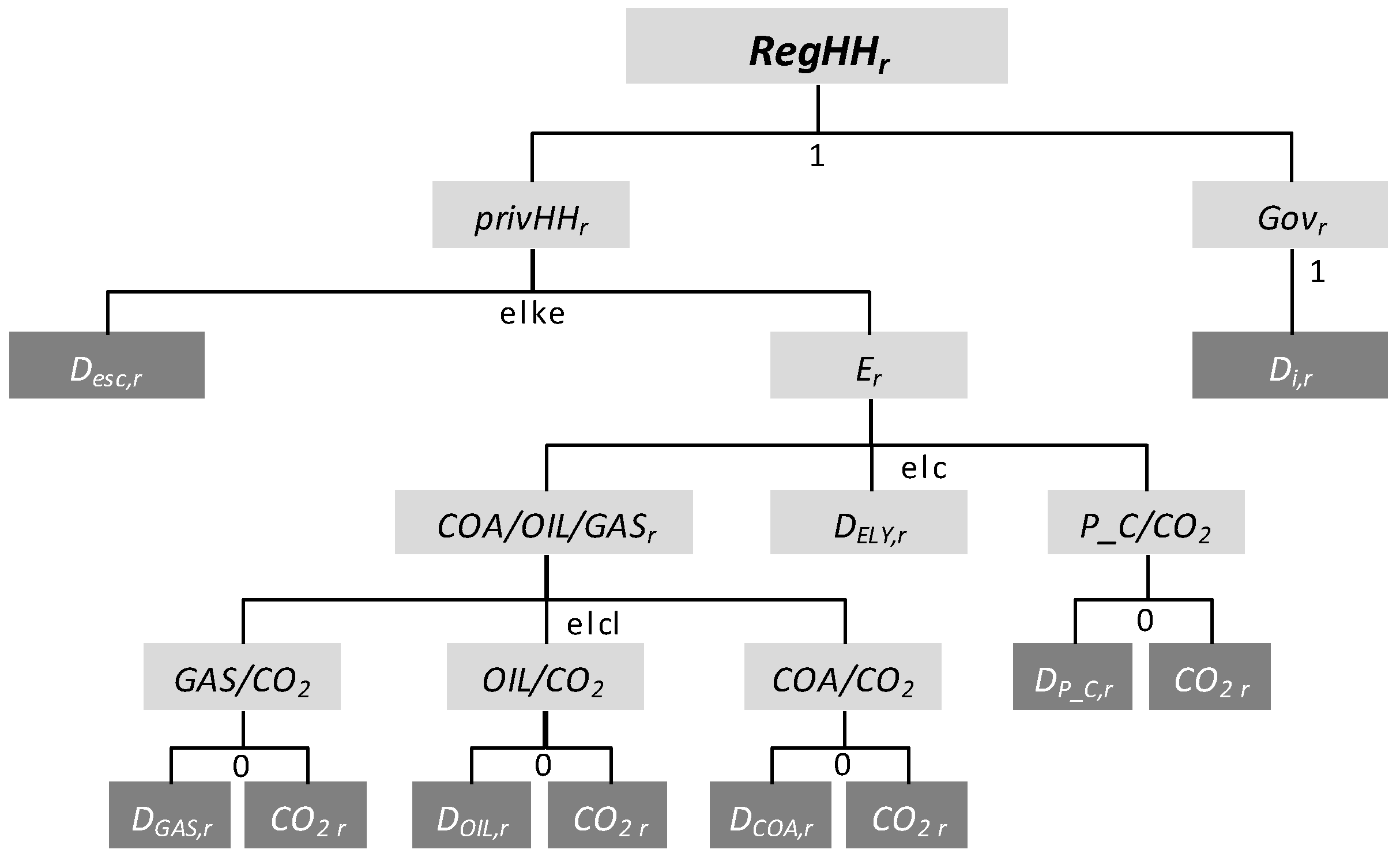
The income for the regional household (RegHHr) in the CGE model is generated by the employment of the primary factors capital (Kr), labor (Lr), and natural resources (Rr), as well as tax revenues. The regional household redistributes this income for the consumption of a representative private household (pirvHHr) and the public consumption of the government (Govr) with a unitary elasticity of substitution. Private consumption in each region is characterized by a constant elasticity of substitution between a material consumption bundle and an energy aggregate. Public consumption is modeled as a Cobb Douglas aggregate of an intermediate material consumption bundle. For this activity, a nested constant elasticity of substitution (CES) function with several levels is employed, which is shown in Figure A1.
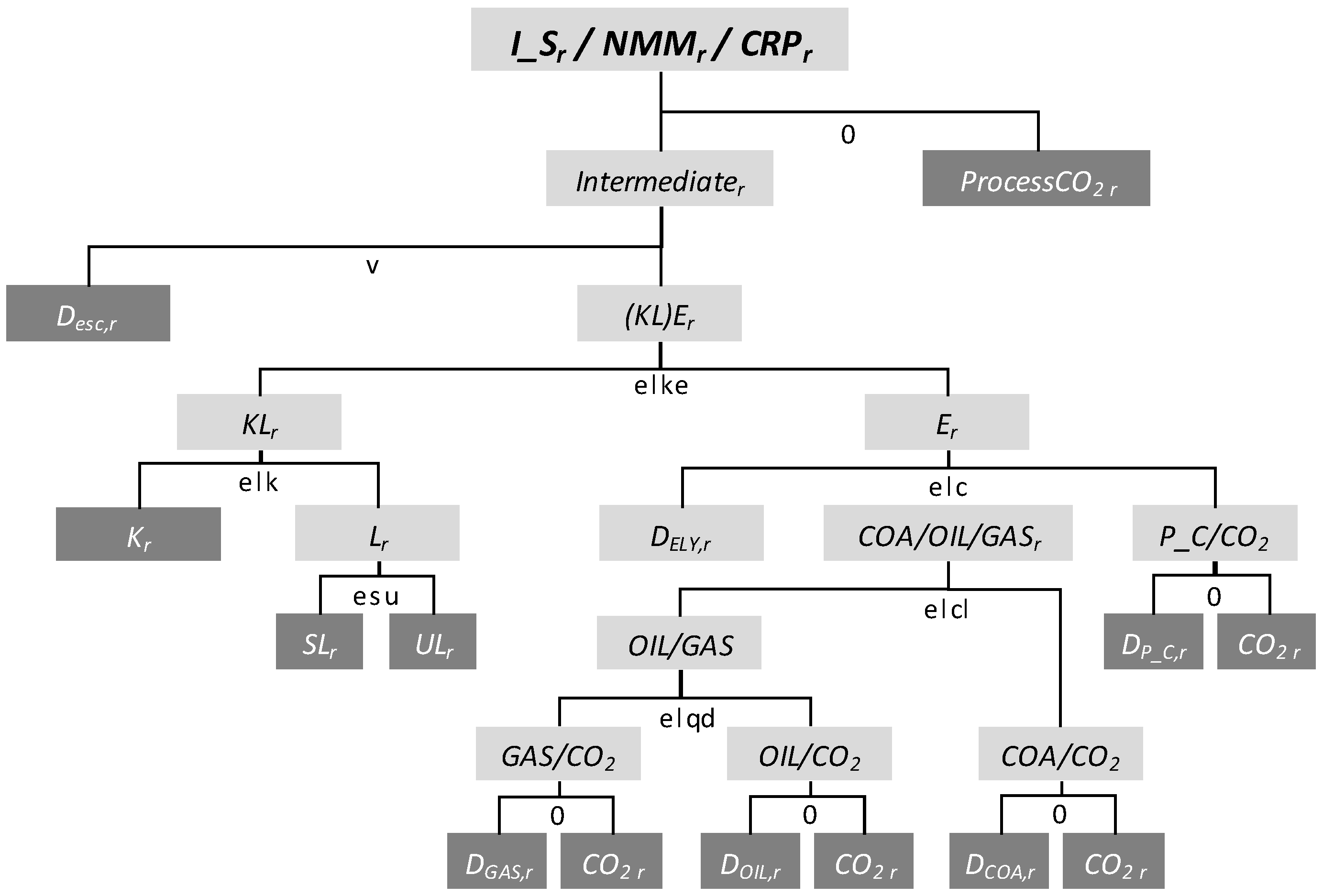
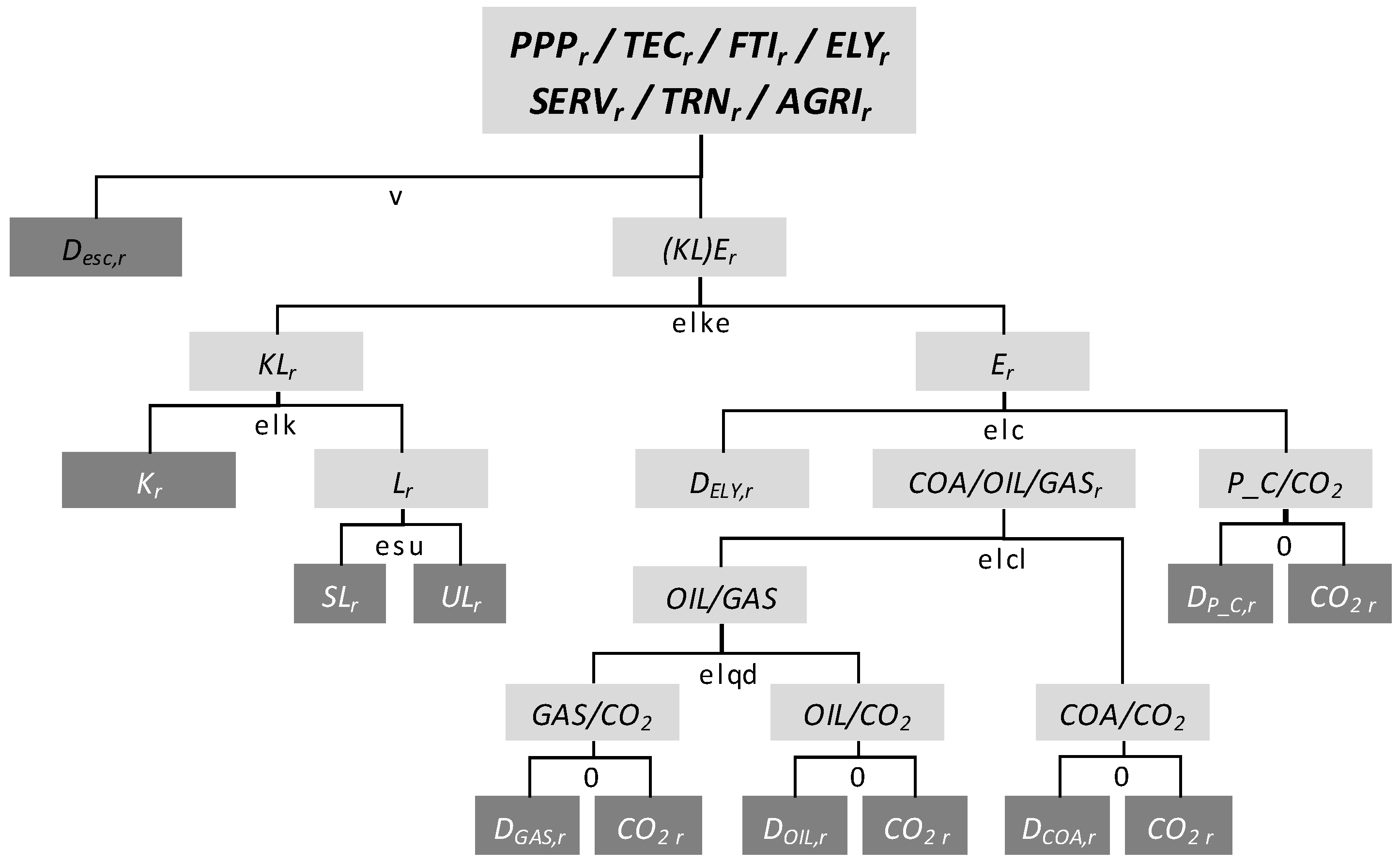
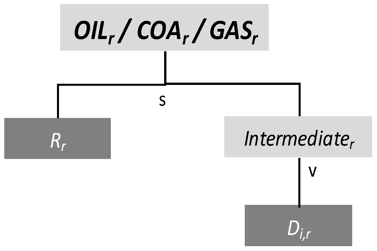
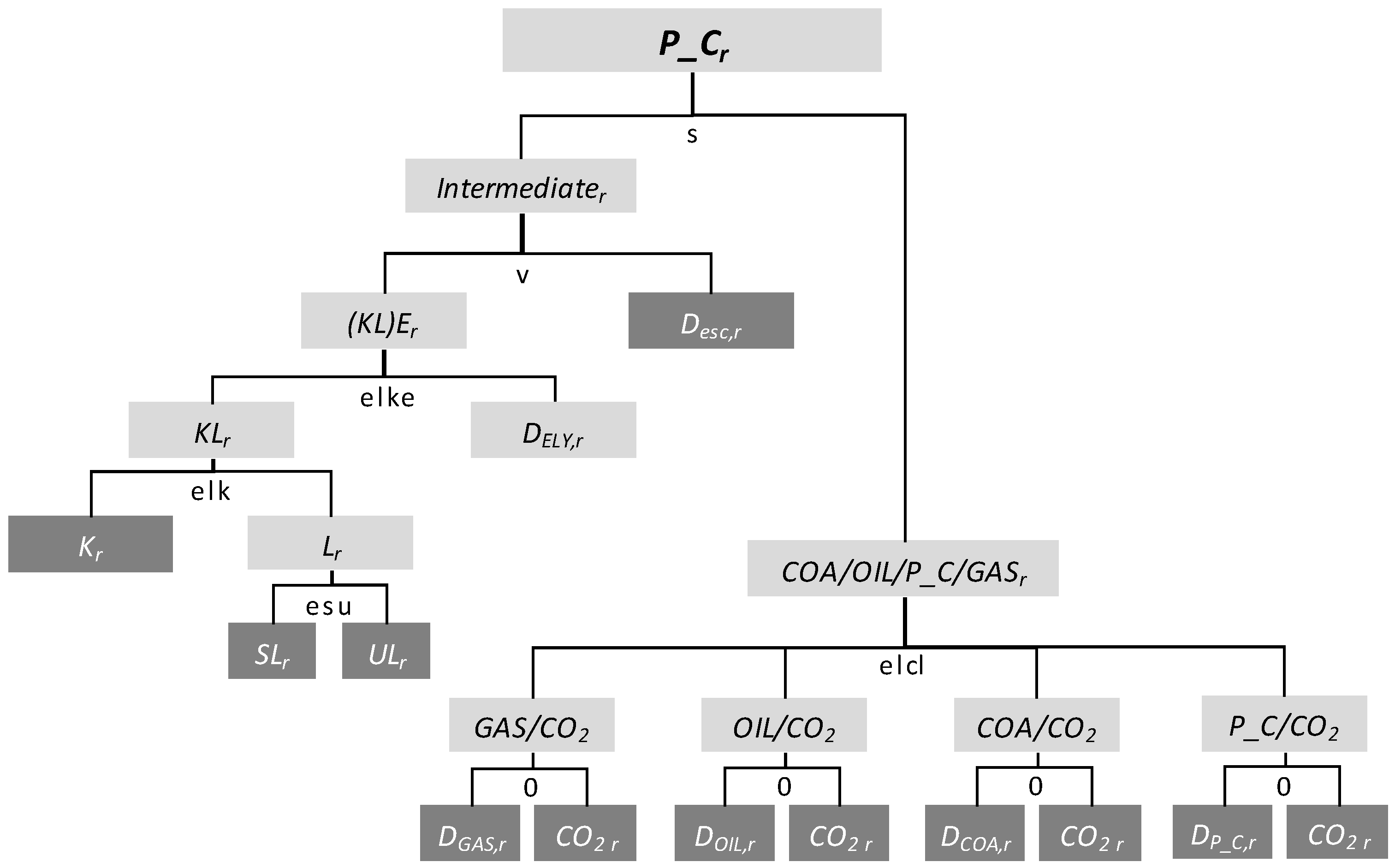
In the domestic production (Yir), intermediate inputs and primary factors are used. The primary factors labor and capital are mobile across sectors within a region but immobile between regions. The natural resource (
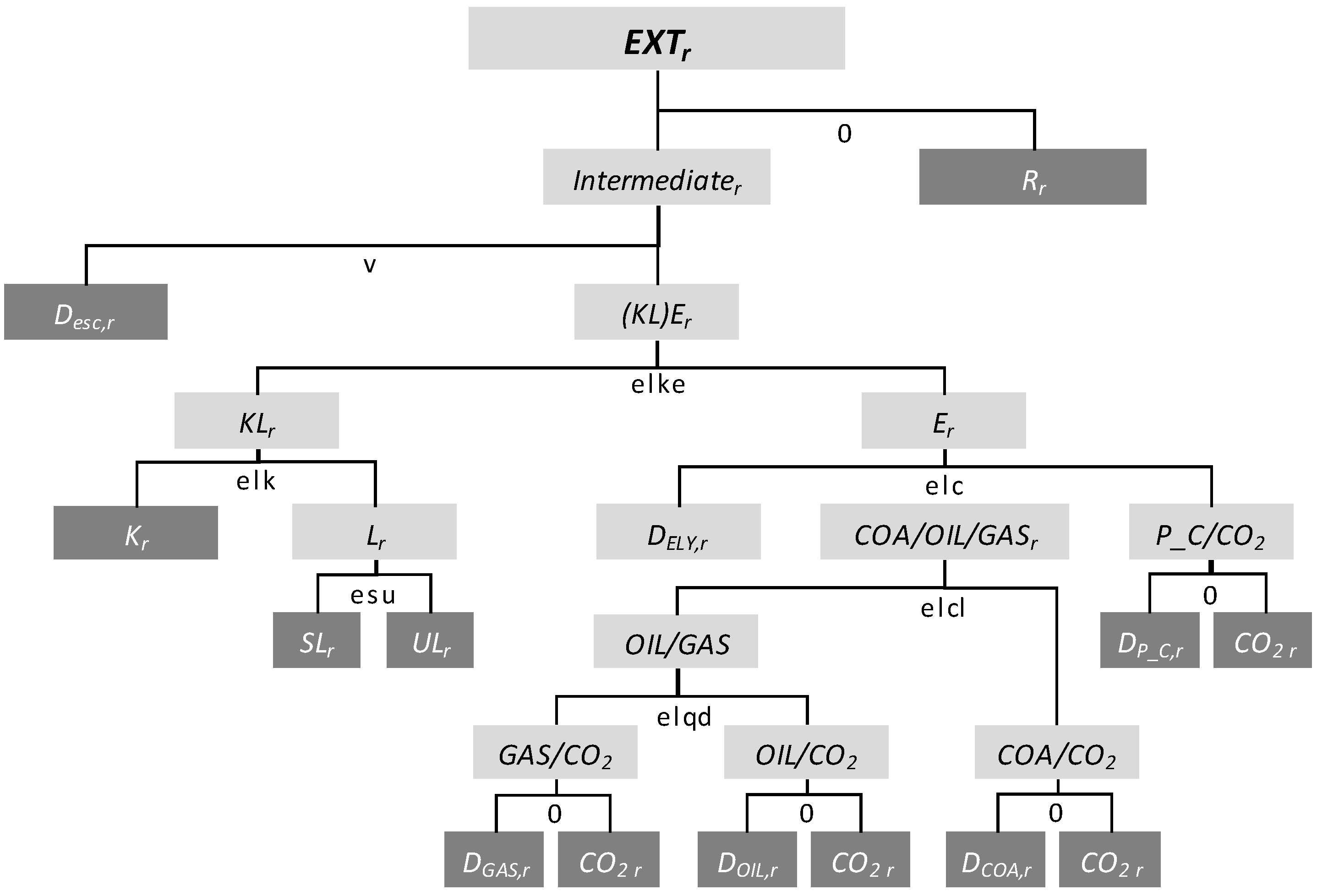
Rr) input is used only in the extraction of primary energy (COA, OIL, and GAS) and Other Extraction (EXT). Again, nested CES production functions are used for the representation of substitution possibilities in domestic production between the primary inputs (capital, labor, and natural resources), intermediate energy and material inputs as well as substitutability between energy commodities (primary and secondary). The domestic production activities Yir are differentiated in three nesting-types of production sectors: (i) non-resource using commodity production (comprising EIS and other NEIS sectors); (ii) resource using (primary energy) extraction sectors; and (iii) the production in the Petroleum sector. The first type of non-resource using production is further divided into production structures that produce process emissions (Figure A2) and those that do not (Figure A3). In addition, the second type of production sectors is represented by the structure of Coal, Crude Oil and Natural Gas production (Figure A4) as well as the Other Extraction sector (Figure A5). Finally, in the Petroleum sector (P_C) the fossil fuel inputs GAS, OIL, COA and P_C are nested in a Leontief type at the top nesting level to all other inputs (i.e., they are characterized by zero elasticity of substitution) such that production cannot substitute away from energy inputs (Figure A6).
Figure A1. Nesting structure of the regional household demand in the CGE model.
Energies 10 00360 g010
Figure A2. Nesting structure of non-resource using sectors with combustion and process emissions in production in the CGE model.
Energies 10 00360 g011
Figure A3. Nesting structure of non-resource using sectors without process emissions in production in the CGE model.
Energies 10 00360 g012
Figure A4. Nesting structure of the resource using fossil fuel sectors without process emissions in production in the CGE model.
Energies 10 00360 g013
Figure A5. Nesting structure of resource using Other Extraction sector without process emissions in production in the CGE model.
Energies 10 00360 g014
Figure A6. Nesting structure of Petroleum (P_C) sector without process emissions in production in the CGE model.
Energies 10 00360 g015
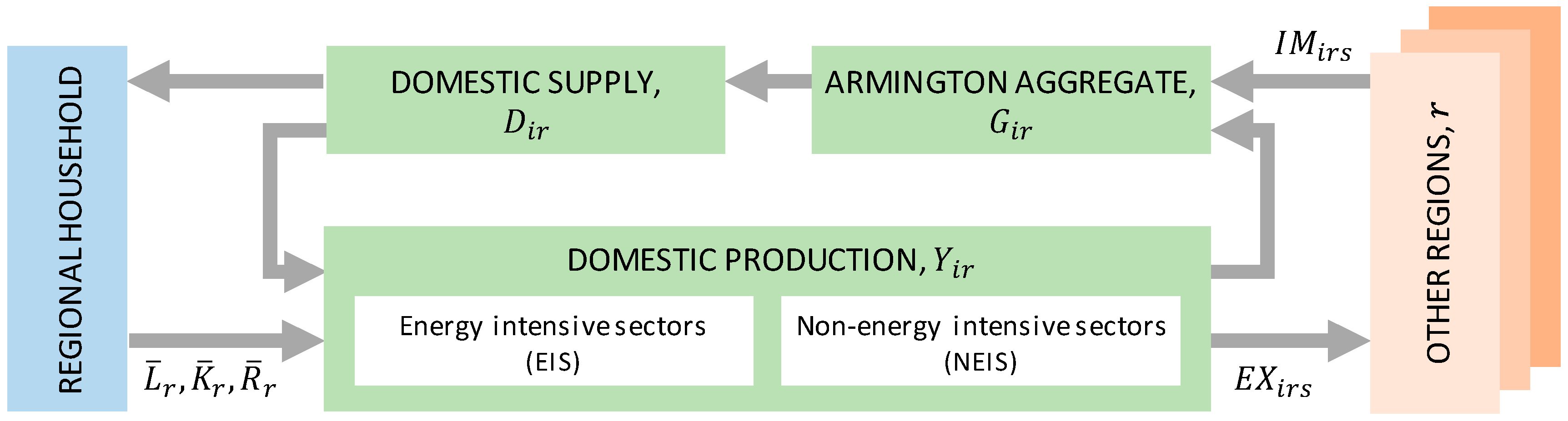
International trade between the 13 regions follows the Armington hypothesis [58], according to which domestic and imported goods are treated as imperfect substitutes. The Armington aggregate Gir is thus implemented as a CES function of domestic production Yir and imported goods IMirs. The output of the Armington aggregate enters the domestic supply Dir, which in turn is used to satisfy final household demand and intermediate demand in production. Each sectoral import of one region from another region corresponds to the respective sectoral export flow of the other region, originating from its domestic production Yir.
CO2 emissions are covered in the CGE model both for production and consumption activities. They are differentiated into combustion and industrial process emissions. The combustion of fossil fuels is modeled as a fixed composite of fossil fuel input and CO2 emission with a fuel specific carbon coefficient. In the three production sectors of Iron and Steel, Non-metallic Minerals and Chemicals industrial process emissions are covered by nesting emissions as Leontief input at the top level of the CES function nesting tree as shown in Figure A2.
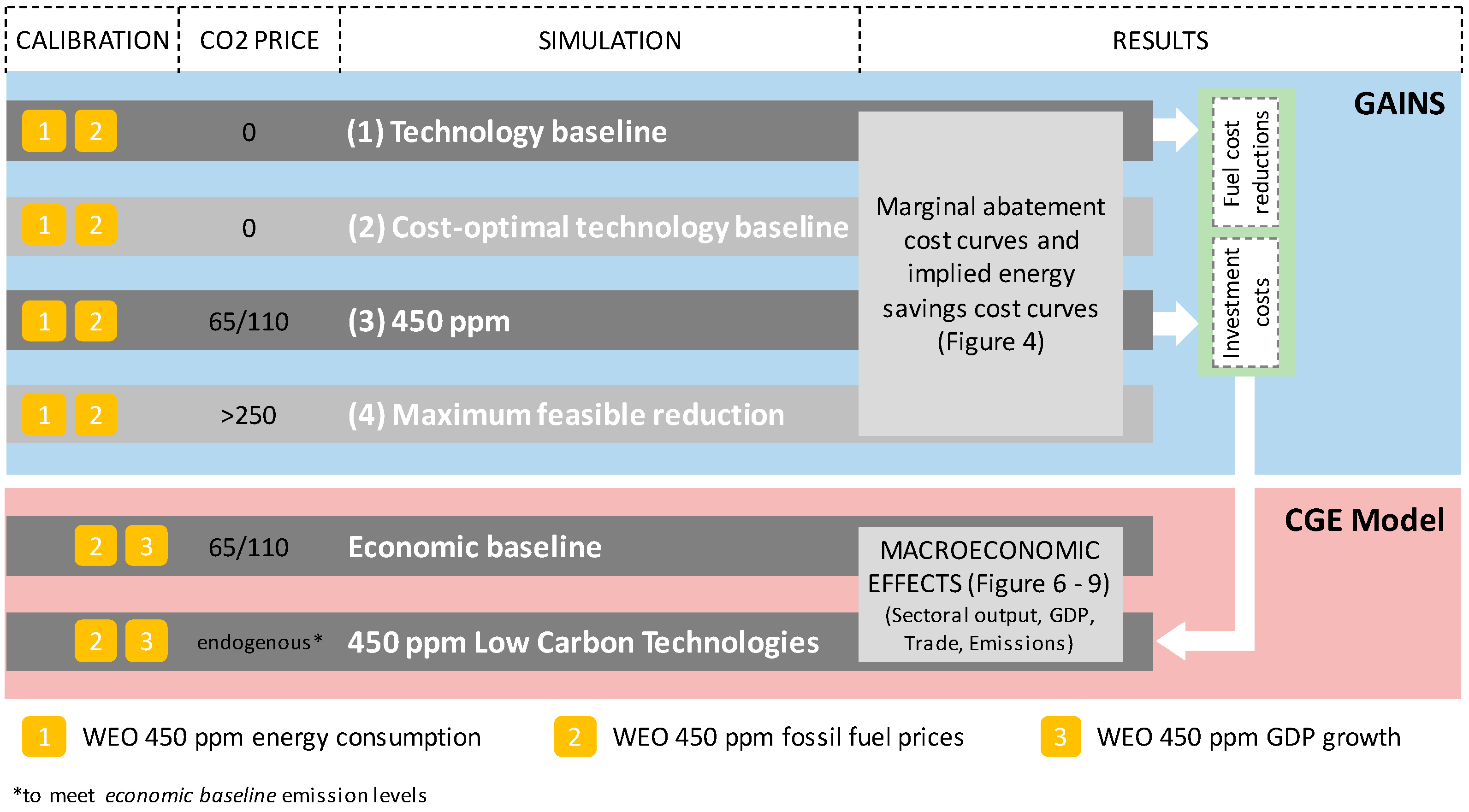
The GAINS model is an integrated assessment model of air pollution and GHG mitigation that covers all sectors of the economy in around 180 regions of the world. The model can be used in a number of different ways, with a focus on economy-wide or sectoral aspects. For example, it can be used calculate sectoral and national/regional/global emissions from an exogenously given energy scenario, such as the WEO. Most pertinent for the current context of industrial emissions, it can also be used to separate the WEO assumptions on projections of production volumes of industrial products from the corresponding average energy intensity per unit of product ( E / U ) for major products i in the energy intensive industries:
E i =   ( E / U ) i ×   P r o d u c t i o n i .
For the present purposes, further enrich the average energy-intensity ( E / U ) i with independent analysis of energy efficiency and cost information of individual technologies, which can be grouped into technology packages. Thus, ( E / U ) i can be expressed as resulting from a mix of technology packages p i , each of which is represented by an implementation rate or weight w p i :
( E U ) i = p i ( E U ) p i × w p i   ,   p i w p i = 1
In practice, we define package p 0 for product i as the set of technologies that describe energy intensity by product i in the base year, i.e., w p 0 i =   1 for all products in the base year, and the other packages describe improvements in this efficiency: in particular, package 1 ( p 1 i ) describes the implication for the average energy intensity across a region of switching off smaller, inefficient production facilities; package 2 ( p 2 i ) represents the implications of reaching the national energy efficiency frontier (best practice at the national level) in all facilities; and package 3 ( p 3 i ) represents reaching the international energy efficiency frontier. As more energy efficient technologies are adopted over time or as a result of a policy intervention, the weights (proxies for levels of implementation) of the more efficient technologies increase and the overall efficiency increases. Simultaneously, because each package is associated with a well-defined unit cost for implementation (which itself is a function of (annualized) investment costs, operating and maintenance costs and fuel costs saved), the change in implementation rates is associated with a change in implementation costs.
In a third step the GAINS model can be used to identify cost-effective strategies to respond to an exogenous policy intervention, in this case a carbon price. For this we set up a linear programming-optimization in which the objective that is minimized is the implementation costs of energy efficiency technologies summed over all subsectors and products, plus the carbon price revenues (carbon price times emissions). The independent variables in this optimization problem are the implementation rates of the efficiency packages, which are subject to the obvious constraint that they sum up to 100% for each product in each subsector, and may be subjective to additional constraints (for example, a share of installations may not be upgradable).
To illustrate the level of disaggregation and detail of input parameters, Table A1 shows—for China—the historical and projected production numbers for the major products in the respective energy intensive industries (products not listed here are subsumed in a category “other” for each subsector, whose trend in production volumes is inferred from the value-added projections for the subsectors).
Table A1. Statistical data and projection of production volumes of the industrial products modeled here for the case of China. Source: [52] and own.
Sector/ProductUnit2005201020202030
Iron and Steel industry
 Coke106 tons254.1 390.2 323.9 209.0
 Sinter and pellets106 tons427.8 642.2 521.0 448.3
 Pig iron106 tons343.8 516.1 418.7 360.3
 Basic oxygen steel106 tons295.4 443.2 359.6 309.4
 Electric arc steel106 tons57.6 86.4 70.1 60.3
 Casting rolling finishing106 tons finished products335.3 503.1 421.0 362.3
Coal production and refineries
 Coal production106 tons2204.7 2584.6 3729.2 4270.2
 Oil refineries106 tons oil input198.4 224.9 301.5 370.0
Chemicals industry
 Ammonia106 tons40.4 49.6 68.4 91.9
 Ethylene106 tons12.2 15.0 29.0 38.9
 Chlorine106 tons14.4 17.7 24.9 33.5
Non-metallic mineral industry
 Cement106 tons1065.8 1700.0 1456.2 1403.0
 Lime106 tons150.9 152.0 154.7 158.0
 Bricks106 tons1040.0 1460.0 1500.0 1500.0
Non-ferrous metals industry
 Primary aluminum106 tons8.5 12.5 14.5 13.0
 Secondary aluminum106 tons0.1 0.1 0.1 0.1
 Other metals—primary106 tons8.6 11.5 12.0 12.0
 Other metals—secondary106 tons8.6 11.5 12.0 12.0
Pulp and Paper industry
 Pulp from wood106 tons10.4 15.5 18.0 18.4
 Pulp from recovered paper106 tons6.9 15.5 33.5 34.1
 Paper and paperboard106 tons14.4 25.8 42.9 43.7
Table A2 shows, for two selected products/production processes of the Iron and Steel industry in China, the energy intensity for different energy carriers and the resulting total for the packages described above. Package 0 represents the average energy efficiency in 2005, and packages 1 to 3 represent clusters of technological measures that reduce the energy intensity at constant output.
Table A2. Energy intensity per unit of output for two selected products in the Iron and Steel sector in China for different energy carriers.
Energy Intensity (GJ per Unit)Package 0Package 1Package 2Package 3
Pig iron production
 Fuels10.59.58.68.0
 Steam hot water0.00.00.00.0
 Electricity0.90.70.60.5
 Total11.410.29.28.5
Electric arc steel
 Fuels1.41.21.00.9
 Steam hot water0.00.00.00.0
 Electricity2.62.21.91.7
 Total4.03.42.92.6
Table A3 illustrates the corresponding cost parameters for the efficiency packages for these two processes. Since we are only interested in costs in addition to baseline costs, we only report investment costs over the Package 0 costs. Differences in operating and maintenance costs can also reflect productivity changes, and these have been reflected to the extent they are included in the more disaggregated marginal cost curves that assume constant output. Regional differences in investment costs are marginal.
Table A3. Cost parameters for the energy efficiency packages discussed in the text above. Since no technological cost learning effect is assumed, these cost parameters are used also for 2030.
Efficiency Package/Cost ParameterUnitPackage 0Package 1Package 2Package 3
Pig iron production
 Capital investments (INV)$/unit-4.130.573.0
 O + M (fixed)% INV-5.0%5.0%5.0%
Electric arc steel
 Capital investments (INV)$/unit-7.116.454.0
 O + M (fixed)% INV-0.0%0.0%0.0%
Finally, Table A4 illustrates our assumed implementation rates of the different packages for selected products in the 2030 technology baseline for China. These implementation rates reflect the reduction in energy intensity autonomously and as a result of non-carbon policies in the technology baseline. In conjunction with the above energy intensities and production volumes, they are consistent with the projected WEO 2009 baseline energy consumption. For India and Europe, processes and energy efficiency packages are not fundamentally different, rather the implementation rates are different (e.g., in Europe zero share for Package 0), reflecting different baseline intensities. Consequently, the remaining per unit potentials for further improvement differ by region. In addition, production volumes differ across regions and products. These differences, taken together, explain the differences in abatement cost curves across regions.
Table A4. Examples of implementation rates of energy efficiency packages in China in the 2030 technology baseline for selected products of the Iron and Steel industry.
Efficiency PackagePackage 0Package 1Package 2Package 3
Pig iron production50%35%10%5%
Electric arc steel60%30%10%0%
Note that the implied cost saving resulting from reduced energy intensity for the higher packages can be inferred from the above energy intensities (Table A1), production volumes, implementation rates and scenario energy prices. Investment requirements are calculated from production volumes, implementation rates and unit investment costs. In the presence of a carbon price the implementation rates change, and the cost-effective levels are determined with an LP-optimization. The results of these calculations are summarized in Figure 3 and Figure 4.
Technology parameters listed in Table A2, Table A3 and Table A4 were discussed with and reviewed by experts in Europe, India and China. In particular, for Europe the GAINS model has benefited from a peer review process in the run up to the policy assessment process leading to the Revision of the Gothenburg Protocol and the Thematic Strategy for Air Pollution of the EU, for both of which the GAINS model was the modeling tool of choice. Many parameters were directly taken or derived from the PRIMES model [59]. For the India and China parts IIASA had subcontracted local experts to review the above methodology and to provide updated parameters. In addition, Zhang et al. [56] provided input from own independent analyses. Cost figures have a local and a world market component (except in cases where no specific information was available), reflecting the fact that (parts of) the technologies are developed and manufactured locally, using local labor and resource costs, while other parts have to be purchased at world market prices. This, and different requirements for the technologies (e.g., different air pollution control requirements), explain cost differentials between technologies in different regions.
Autonomous technological improvement is already reflected in the WEO as decreasing average energy intensities for the individual products over time. In GAINS, this is represented by increasing implementation rates of the higher stage packages. No technological learning is assumed here, in the sense that the unit costs for the technology packages and their energy efficiency stay constant over time. While this may be a relatively conservative assumption, the impact of learning in these mature industries is considered relatively small, compared to younger industries such as those producing, for instance, computer hardware or solar PV modules.

Appendix B. Model Calibration

As described in Section 2.3, we calibrate our models to the assumptions of the WEO 2009 450 scenario. In detail, for the technology baseline of the GAINS model, we calibrate the energy consumption (Table 9.2, p. 324, [52]) as well as the fossil fuel prices (Table 4, p. 64, [52]) for each region. GAINS imports IEA WEO fuel consumption and industrial production data directly from spreadsheets provided by the IEA. Those include, but are not restricted to the data found in the print version of the WEO modeling results. In the GAINS 450 ppm simulation we additionally implement a carbon price of 110 USD/tCO2e and 65 USD/tCO2e for Annex I and non-Annex I regions and adjusted costs and potentials of the mitigation options in each sector to be consistent with the energy consumption of the WEO 2009 450 scenario.
The economic baseline in the CGE model is calibrated to the regional GDP growth rates from the WEO 2009 (Table 3, p. 62, [52]), by proportional augmentation of regional household endowments of unskilled labor, skilled labor, capital and CGDS. For the additional calibration to the fossil fuel prices from the WEO 2009 (Table 4, p. 64, [52]), fuel prices were exogenously fixed in the first place. Then, we fix resource supplies and recalibrate the substitution elasticities in the fossil fuel sectors to specify the price elasticities. The carbon price of 110 USD/tCO2e and 65 USD/tCO2e for Annex I and non-Annex I regions is implemented by an endogenous reduction of carbon endowments of the regional households to the exogenous carbon price.

Appendix C. Sensitivity Analysis

To assess the reliability of our analysis results we perform a sensitivity analysis, testing different parameters in our modeling framework. We investigate the sensitivity of macroeconomic values presented in Section 4 to parameter variations in the technology framework, the macroeconomic framework, the model link and the scenario calibration. Specifically, we simulate: (1) a simultaneous variation in fossil fuel input reductions in each energy intensive industry; (2) a simultaneous variation in sectoral input substitution elasticities in all regions; (3) a simultaneous variation in sectoral import transformation elasticities of Armington Aggregate in all regions; (4) a simultaneous variation of depreciation time of investment for all low carbon technologies; and (5) a simultaneous variation of carbon price in Annex I and non-Annex I regions in economic baseline and 450 ppm low carbon technologies scenario. We vary each of the parameters in the range of 50% to 200%. Table A5 shows the absolute minimum (lower bound) and maximum (upper bound) of all the simulations compared to the base results presented in Section 4. The numbers are given for sectoral output in energy intensive sectors, as well as the macroeconomic indicators of total regional output, GDP and total regional CO2 emissions for Europe, China and India.
Table A5. Upper and lower bound of simulation results in sensitivity analysis for main indicators in Europe, China and India.
IndicatorLower BoundBaseUpper Bound
Europe
 Petroleum−44.39%−22.88%−5.72%
 Electricity1.54%4.10%8.20%
 Iron and Steel−6.23%−1.98%0.00%
 Non-metallic Minerals−4.34%−1.75%−0.58%
 Paper and Pulp−4.80%−1.91%−0.79%
 Chemicals−15.95%−6.47%−3.44%
 Total Output−3.20%−1.40%−0.44%
 GDP−4.25%−0.81%0.15%
 Total CO2−17.02%−14.21%−10.00%
China
 Petroleum12.36%15.72%44.84%
 Electricity21.36%26.78%36.54%
 Iron and Steel−3.08%4.35%6.22%
 Non-metallic Minerals6.09%9.60%14.06%
 Paper and Pulp−0.13%5.16%7.68%
 Chemicals−0.79%6.09%8.42%
 Total Output−0.11%2.69%5.67%
 GDP0.10%3.01%7.84%
 Total CO2−18.95%−9.87%−4.08%
India
 Petroleum6.51%12.59%25.91%
 Electricity17.43%22.65%29.27%
 Iron and Steel−4.46%1.94%3.21%
 Non-metallic Minerals3.46%8.07%10.83%
 Paper and Pulp5.50%7.98%11.64%
 Chemicals5.98%17.30%35.26%
 Total Output0.03%2.14%4.70%
 GDP0.20%3.19%6.99%
 Total CO2−21.26%−11.85%−3.05%
Despite the variation in the results for Europe, there is no change in the direction of any indicator except for GDP in the upper bound, for which a slightly positive effect results from a doubled life-time of low carbon investments. The results for China also show a sensitivity that switches the direction of effects only in the case of a halving of life-time of low carbon technologies. In India, output in the Iron and Steel sector is most sensitive to parameter variations. Overall, the results appear to be robust across the tested parameter variations and now show contradiction to our main findings.

Appendix D. Sectoral Output Decomposition

The decomposition of total sectoral output effects was carried out in several model simulations assuming low carbon technology deployment in each of the energy intensive sectors only and in all sectors simultaneously. The decomposition can be formalized in the following equation.
Δ O i = Δ O i j + Δ E X i j + Δ I M i j + ( Δ O i a l l t e c h Δ O i j ) ; i = ( p c , e l y ,   i s , n m m ,   p p p ,   c r p ) ; j = ( p c , e l y ,   i s , n m m ,   p p p ,   c r p )
The index i indicates the sectoral effect within a simulation run, while the index j denotes the simulation run characterized by the sector in which a deployment of low carbon technologies is assumed.

References

  1. International Energy Agency (IEA). Energy Technology Perspectives 2010: Scenarios & Strategies to 2050; International Energy Agency: Paris, France, 2010. [Google Scholar]
  2. Allwood, J.M.; Cullen, J.M.; Milford, R.L. Options for Achieving a 50% Cut in Industrial Carbon Emissions by 2050. Environ. Sci. Technol. 2010, 44, 1888–1894. [Google Scholar] [CrossRef] [PubMed]
  3. International Energy Agency (IEA). Energy Efficiency Market Report 2016; International Energy Agency: Paris, France, 2016. [Google Scholar]
  4. Napp, T.A.; Gambhir, A.; Hills, T.P.; Florin, N.; Fennell, P.S. A review of the technologies, economics and policy instruments for decarbonising energy-intensive manufacturing industries. Renew. Sustain. Energy Rev. 2014, 30, 616–640. [Google Scholar] [CrossRef]
  5. Morrow, W.R.; Hasanbeigi, A.; Sathaye, J.; Xu, T. Assessment of energy efficiency improvement and CO2 emission reduction potentials in India’s cement and iron & steel industries. J. Clean. Prod. 2014, 65, 131–141. [Google Scholar]
  6. Quader, M.A.; Ahmed, S.; Ghazilla, R.A.R.; Ahmed, S.; Dahari, M. A comprehensive review on energy efficient CO2 breakthrough technologies for sustainable green iron and steel manufacturing. Renew. Sustain. Energy Rev. 2015, 50, 594–614. [Google Scholar] [CrossRef]
  7. Birat, J.P.; Brolée, J.; Korthas, B.; van der Stel, J.; Meijer, K.; Günther, C.; Halin, M.; Bürgler, T.; Lavelaine, H.; Treadgold, C.; et al. ULCOS Program: A Progress Report in the Spring of 2008. In Proceedings of the 3rd International Conference on Process Development in Iron and Steelmaking, Luleå, Sweden, 8–11 June 2008.
  8. International Energy Agency (IEA). Technology Roadmap: Wind Energy; International Energy Agency: Paris, France, 2013. [Google Scholar]
  9. International Energy Agency (IEA). Technology Roadmap: Solar Photovoltaic Energy; International Energy Agency: Paris, France, 2014. [Google Scholar]
  10. Romeo, L.M.; Catalina, D.; Lisbona, P.; Lara, Y.; Martínez, A. Reduction of greenhouse gas emissions by integration of cement plants, power plants, and CO2 capture systems. Greenh. Gas Sci. Technol. 2011, 1, 72–82. [Google Scholar] [CrossRef]
  11. Peters, G.P.; Minx, J.C.; Weber, C.L.; Edenhofer, O. Growth in emission transfers via international trade from 1990 to 2008. Proc. Natl. Acad. Sci. USA 2011, 108, 8903–8908. [Google Scholar] [CrossRef] [PubMed]
  12. European Commission COMMISSION DECISION of 27 October 2014 Determining, Pursuant to Directive 2003/87/EC of the European Parliament and of the Council, a List of Sectors and Subsectors Which are Deemed to be Exposed to a Significant Risk of Carbon Leakage, for the Period 2015 to 2019. Available online: http://eur-lex.europa.eu/legal-content/EN/ALL/?uri=CELEX%3A32014D0746 (accessed on 3 March 2017).
  13. Arens, M.; Worrell, E.; Eichhammer, W.; Hasanbeigi, A.; Zhang, Q. Pathways to a low-carbon iron and steel industry in the medium-term—The case of Germany. J. Clean. Prod. 2016. [Google Scholar] [CrossRef]
  14. Hasanbeigi, A.; Arens, M.; Price, L. Alternative emerging ironmaking technologies for energy-efficiency and carbon dioxide emissions reduction: A technical review. Renew. Sustain. Energy Rev. 2014, 33, 645–658. [Google Scholar] [CrossRef]
  15. Pardo, N.; Moya, J.A. Prospective scenarios on energy efficiency and CO2 emissions in the European Iron & Steel industry. Energy 2013, 54, 113–128. [Google Scholar]
  16. Huang, Y.-H.; Chang, Y.-L.; Fleiter, T. A critical analysis of energy efficiency improvement potentials in Taiwan’s cement industry. Energy Policy 2016, 96, 14–26. [Google Scholar] [CrossRef]
  17. Xu, J.-H.; Fleiter, T.; Fan, Y.; Eichhammer, W. CO2 emissions reduction potential in China’s cement industry compared to IEA’s Cement Technology Roadmap up to 2050. Appl. Energy 2014, 130, 592–602. [Google Scholar] [CrossRef]
  18. Hanaoka, T.; Kainuma, M. Low-carbon transitions in world regions: Comparison of technological mitigation potential and costs in 2020 and 2030 through bottom-up analyses. Sustain. Sci. 2012, 7, 117–137. [Google Scholar] [CrossRef]
  19. Broberg, T.; Berg, C.; Samakovlis, E. The economy-wide rebound effect from improved energy efficiency in Swedish industries—A general equilibrium analysis. Energy Policy 2015, 83, 26–37. [Google Scholar] [CrossRef]
  20. Allan, G.; Hanley, N.; McGregor, P.; Swales, K.; Turner, K. The impact of increased efficiency in the industrial use of energy: A computable general equilibrium analysis for the United Kingdom. Energy Econ. 2007, 29, 779–798. [Google Scholar] [CrossRef]
  21. Hanley, N.D.; McGregor, P.G.; Swales, J.K.; Turner, K. The impact of a stimulus to energy efficiency on the economy and the environment: A regional computable general equilibrium analysis. Renew. Energy 2006, 31, 161–171. [Google Scholar] [CrossRef]
  22. Schinko, T.; Bednar-Friedl, B.; Steininger, K.; Grossmann, W. Switching to carbon-free production processes: Implications for carbon leakage and border carbon adjustment. Energy Policy 2014, 67, 818–831. [Google Scholar] [CrossRef]
  23. Cai, Y.; Arora, V. Disaggregating electricity generation technologies in CGE models: A revised technology bundle approach with an application to the U.S. Clean Power Plan. Appl. Energy 2015, 154, 543–555. [Google Scholar] [CrossRef]
  24. Schumacher, K.; Sands, R.D. Where are the industrial technologies in energy-economy models? An innovative CGE approach for steel production in Germany. Energy Econ. 2007, 29, 799–825. [Google Scholar] [CrossRef]
  25. Laitner, J.A.; Hanson, D.A. Modeling detailed energ-efficiency technologies and technology policies within a CGE framework. Energy J. 2006, 27, 151–169. [Google Scholar]
  26. Lanz, B.; Rausch, S. General equilibrium, electricity generation technologies and the cost of carbon abatement: A structural sensitivity analysis. Energy Econ. 2011, 33, 1035–1047. [Google Scholar] [CrossRef]
  27. Böhringer, C.; Rutherford, T. Combining bottom-up and top-down. Energy Econ. 2008, 30, 574–596. [Google Scholar] [CrossRef]
  28. Sue Wing, I. The synthesis of bottom-up and top-down approaches to climate policy modeling: Electric power technology detail in a social accounting framework. Energy Econ. 2008, 30, 547–573. [Google Scholar] [CrossRef]
  29. Hourcade, J.C.; Jaccard, M.; Bataille, C.; Ghersi, F. Hybrid Modeling: New Answers to Old Challenges. Energy J. 2006, 2, 1–12. [Google Scholar]
  30. Schäfer, A.; Jacoby, H.D. Technology detail in a multisector CGE model: Transport under climate policy. Energy Econ. 2005, 27, 1–24. [Google Scholar] [CrossRef]
  31. Messner, S.; Schrattenholzer, L. MESSAGE-MACRO: Linking an energy supply model with a macroeconomic module and solving it iteratively. Energy 2000, 25, 267–282. [Google Scholar] [CrossRef]
  32. Edenhofer, O.; Knopf, B.; Barker, T.; Baumstark, L.; Bellevrat, E.; Chateau, B.; Criqui, P.; Isaac, M.; Kitous, A.; Kypreos, S.; et al. The economics of low stabilization: Model comparison of mitigation strategies and costs. Energy J. 2010, 31, 11–48. [Google Scholar] [CrossRef]
  33. Wagner, F.; Amann, M.; Borken-Kleefeld, J.; Cofala, J.; Höglund-Isaksson, L.; Purohit, P.; Rafaj, P.; Schöpp, W.; Winiwarter, W. Sectoral marginal abatement cost curves: Implications for mitigation pledges and air pollution co-benefits for Annex I countries. Sustain. Sci. 2012, 7, 169–184. [Google Scholar] [CrossRef]
  34. International Energy Agency (IEA). Energy Efficiency Market Report 2013: Market Trends and Medium-Term Prospects; International Energy Agency: Paris, France, 2013. [Google Scholar]
  35. Wang, X.; Lin, B. How to reduce CO2 emissions in China’s iron and steel industry. Renew. Sustain. Energy Rev. 2016, 57, 1496–1505. [Google Scholar] [CrossRef]
  36. International Energy Agency (IEA). Indian Energy Outlook; International Energy Agency: Paris, France, 2015. [Google Scholar]
  37. Amann, M.; Bertok, I.; Borken-Kleefeld, J.; Cofala, J.; Heyes, C.; Höglund-Isaksson, L.; Klimont, Z.; Nguyen, B.; Posch, M.; Rafaj, P.; et al. Cost-effective control of air quality and greenhouse gases in Europe: Modeling and policy applications. Environ. Model. Softw. 2011, 26, 1489–1501. [Google Scholar] [CrossRef]
  38. Wagner, F.; Heyes, C.; Klimont, Z.; Schöpp, W. The GAINS Optimization Module: Identifying Cost-Effective Measures for Improving Air Quality and Short-Term Climate Forcing; International Institute for Applied Systems Analysis (IIASA): Laxenburg, Austria, 2013. [Google Scholar]
  39. Winiwarter, W.; Höglund-Isaksson, L.; Schöpp, W.; Tohka, A.; Wagner, F.; Amann, M. Emission mitigation potentials and costs for non-CO2 greenhouse gases in Annex-I countries according to the GAINS model. J. Integr. Environ. Sci. 2010, 7, 235–243. [Google Scholar] [CrossRef]
  40. Bednar-Friedl, B.; Kulmer, V.; Schinko, T. The effectiveness of anti-leakage policies in the European Union: Results for Austria. Empirica 2012, 39, 233–260. [Google Scholar] [CrossRef]
  41. Bednar-Friedl, B.; Schinko, T.; Steininger, K. The relevance of process emissions for carbon leakage: A comparison of unilateral climate policy options with and without border carbon adjustment. Energy Econ. 2012, 34, 168–180. [Google Scholar] [CrossRef]
  42. Global Trade, Assistance, and Production: The GTAP 8 Data BaseCenter for Global Trade Analysis, Purdue University; Narayanan, B.; Aguiar, A.; McDougall, R. (Eds.) Center for Global Trade Analysis, Purdue University: West Lafayette, IN, USA, 2012.
  43. Lee, H.-L. The Combustion-Based CO2 Emissions Data for GTAP Version 7 Data Base. Available online: http://www.gtap.agecon.purdue.edu/resources/res_display.asp?RecordID=1143 (accessed on 18 July 2013).
  44. UNFCCC Greenhouse Gas Inventory Data. Available online: http://unfccc.int/ghg_data/items/3800.php (accessed on 17 January 2016).
  45. Amann, M.; Rafaj, P.; Hoehne, N. GHG Mitigation Potentials in Annex I Countries. Comparison of Model Estimates for 2020; International Institute for Applied Systems Analysis: Laxenburg, Austria, 2009. [Google Scholar]
  46. Höglund-Isaksson, L.; Winiwarter, W.; Wagner, F.; Klimont, Z.; Amann, M. Potentials and Costs for Mitigation of Non-CO2 Greenhouse Gas Emissions in the European Union until 2030 Results; International Institute for Applied Systems Analysis (IIASA): Laxenburg, Austria, 2010. [Google Scholar]
  47. Nguyen, T.B.; Hoeglund-Isaksson, L.; Wagner, F.; Schoepp, W. Mitigation Efforts Calculator (MEC). Inf. Syst. Front. 2012, 15, 223–233. [Google Scholar] [CrossRef]
  48. Purohit, P.; Amann, M.; Mathur, R.; Gupta, I.; Marwah, S.; Verma, V.; Bertok, I.; Borken, J.; Chambers, A.; Cofala, J.; et al. GAINS ASIA: Scenarios for Cost-Effective Control of Air Pollution and Greenhouse Gases in India; International Institute for Applied Systems Analysis (IIASA): Laxenburg, Austria, 2010. [Google Scholar]
  49. Wagner, F.; Amann, M.; Schöpp, W. The GAINS Optimization Module as of 1 February 2007; International Institute for Applied Systems Analysis (IIASA): Laxenburg, Austria, 2007. [Google Scholar]
  50. E3MLab/ICCS. PRIMES MODEL 2013–2014: Detailed Model Description; National Technical University of Athens: Athens, Greece, 2014. [Google Scholar]
  51. Enerdata POLES: Prospective Outlook on Long-Term Energy Systems. Available online: http://www.enerdata.net/enerdatauk/solutions/energy-models/poles-model.php (accessed on 3 March 2017).
  52. International Energy Agency (IEA). World Energy Outlook 2009; International Energy Agency: Paris, France, 2009. [Google Scholar]
  53. Wagner, F.; Cofala, J. Marginal Abatement Cost Curves for Selected Industry Sectors; International Institute for Applied Systems Analysis (IIASA): Laxenburg, Austria, 2015. [Google Scholar]
  54. Zhao, X.; Ma, C.; Hong, D. Why did China’s energy intensity increase during 1998–2006: Decomposition and policy analysis. Energy Policy 2010, 38, 1379–1388. [Google Scholar] [CrossRef]
  55. Liu, N.; Ma, Z.; Kang, J. Changes in carbon intensity in China’s industrial sector: Decomposition and attribution analysis. Energy Policy 2015, 87, 28–38. [Google Scholar] [CrossRef]
  56. Zhang, S. Energy Efficiency for Clean Air—Capturing the Multiple Benefits for Climate, Air Quality, and Public Health in China. Ph.D. Thesis, Utrecht University, Utrecht, The Netherlands, 2016. [Google Scholar]
  57. International Energy Agency (IEA). World Energy Outlook Special Report 2016: Energy and Air Pollution; International Energy Agency: Paris, France, 2016. [Google Scholar]
  58. Armington, P.S. A Theory of Demand for Products Distinguished by Place of Production. Staff Pap. 1969, 16, 159–176. [Google Scholar] [CrossRef]
  59. Capros, P.; Tasios, N.; De Vita, A.; Mantzos, L.; Paroussos, L. Model-based analysis of decarbonizing the EU economy in the time horizon to 2050. Energy Strategy Rev. 2012, 1, 76–84. [Google Scholar] [CrossRef]
Figure 1. Methodological approach of GAINS technology model and macroeconomic CGE model linking.
Energies 10 00360 g001
Figure 2. Economic structure of each region in the CGE model.
Energies 10 00360 g002
Figure 3. Overview of model calibration and simulations in the technology framework and macroeconomic framework.
Energies 10 00360 g003
Figure 4. Total investment requirements in million USD (a) and reduced fuel costs in million USD per year (b) resulting from energy efficiency measures in different industrial sectors in 2030 as a function of an exogenous carbon price (USD/tCO2e).
Energies 10 00360 g004
Figure 5. Implemented relative input changes for fossil fuels (Coal, Oil, and Gas), Petroleum, and Capital use, as well as unit cost changes in energy intensive sectors in CGE model for 450 ppm low carbon technologies scenario in Europe, China and India. Percentage deviation relative to economic baseline technology in 2030 (based on [53]).
Energies 10 00360 g005
Figure 6. Sectoral and total output effects in energy intensive sectors in Europe, China and India in 2030 for low carbon technology scenario relative to baseline triggered by change in domestic demand (Δdom), change in imports (ΔIM), change in exports (ΔEX), and deployment of low carbon technologies in other sectors (Δall tec).
Energies 10 00360 g006
Figure 7. Effects on total output (EIS = energy intensive sectors; and NEIS = non-energy intensive sectors) by region (ROW = rest of the world) in 2030 for low carbon technology scenario relative to baseline; decomposition into effects of domestic technology investment (Δdom) and technology investment in all regions (Δall).
Energies 10 00360 g007
Figure 8. Change in total export flows between Europe, China, India and rest of the world (ROW) for low carbon technology scenario relative to baseline in billion USD.
Energies 10 00360 g008
Figure 9. Change in CO2 emissions by region in 2030 for low carbon technology scenario relative to economic baseline: in energy intensive (EIS) and non-energy intensive (NEIS) sectors (a); and triggered by sectoral low carbon technology (b).
Energies 10 00360 g009
Table 1. Regional aggregation in the CGE model.
No.Aggregated RegionModel Code
1Central EU 27 + SwitzerlandCEU
2Mediterranean EU 27MEU
3Northern EU 27 + Norway, Liechtenstein and IcelandNEU
4ChinaCHN
5IndiaIND
6Southeastern and Rest of EuropeSROE
7North AmericaNAM
8Rest of industrialized countriesROI
9Other emerging economies ECO
10Latin America (w.o. Brazil, Ecuador and Venezuela)LAM
11Oil and gas exporting countriesOIGA
12Rest of South and South East AsiaRASI
13AfricaAFR
Table 2. Sectoral dimension of the CGE model. Source: GTAP8 [42].
Aggregated SectorsComprising GTAP8 Sectors (GTAP Sector-Number)Model Code
Energy IntensiveEIS
1Petroleummanufacture of coke oven- and refined oil products (32)P_C
2Electricityproduction, collection and distribution of electricity (43)ELY
3Iron and Steelmanufacture of basic iron and steel and casting (35)I_S
4Non-metallic Mineralsmanufacture of cement, plaster, lime, gravel, concrete (34)NMM
5Paper and Pulpmanufacture of paper , pulp and paper products (31)PPP
6Chemicalsmanufacture of basic chemicals, other chemical, rubber and plastics products (33)CRP
Non-Energy IntensiveNEIS
7Agricultureall agriculture sectors (1–12)AGRI
8Food and Textiletextiles (27), wearing apparel (28), leather (29), wood products (30), all food processing sectors (19–26)FTI
9Coalcoal mining (15)COA
10Crude Oiloil extraction (16)OIL
11Natural Gasnatural gas extraction (17), manufacture and distribution of gas, steam and hot water supply (44)GAS
12Other Extractionother mining (18), forestry (13) and fishing (14)EXT
13Technology Industriesprecious and non-ferrous metals (36), fabricated metal products (37), motor vehicles (38), transport equipment (39), communication equipment (40), machinery (41), other manufacturing and recycling (42)TEC
14Other Serviceswater (45), construction (46), wholesale and retail sale, hotels and restaurant (47), post and telecom (51), financial services (52), insurance (53), real estate and other business (54), Recreational and service activities (55), public administration (56), dwellings (57)SERV
15Transportroad, rail, pipeline and other transport (48), water transport (49), Air transport (50)TRN
16Capital Goodscapital goodsCGDS

