
Neuro-Fuzzy Wavelet Based Adaptive MPPT Algorithm for Photovoltaic Systems

 , and
, and
Abstract
:1. Introduction
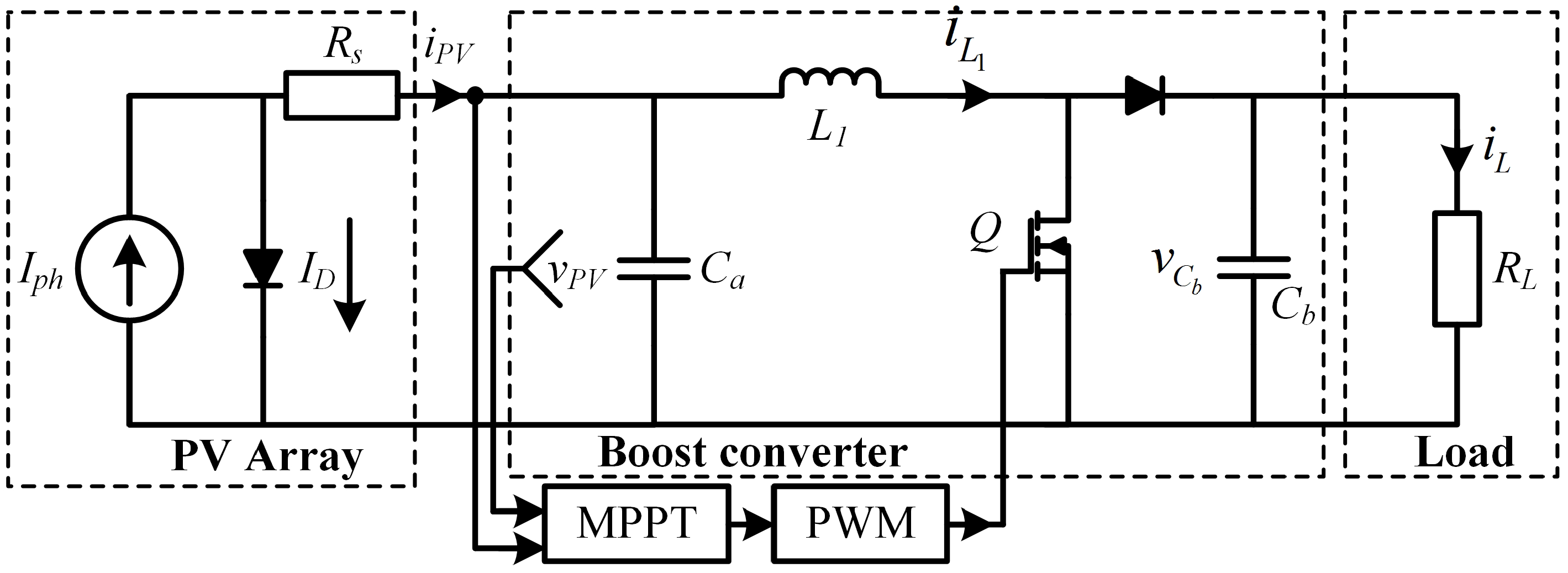
2. Photovoltaic Energy System
2.1. Photovoltaic Array
2.2. DC-DC Boost Converter
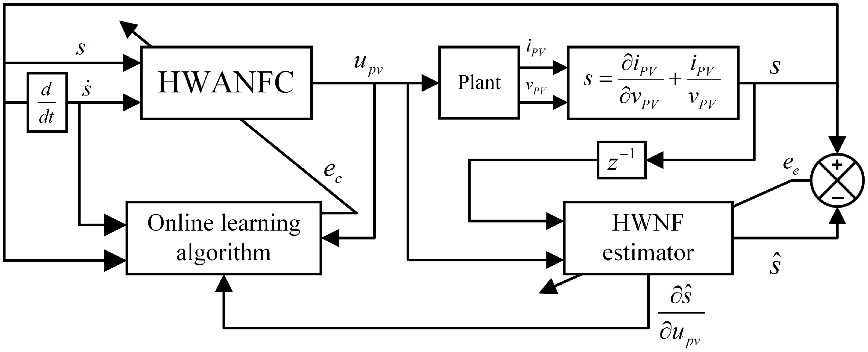
3. Proposed Adaptive Neural Fuzzy Control System
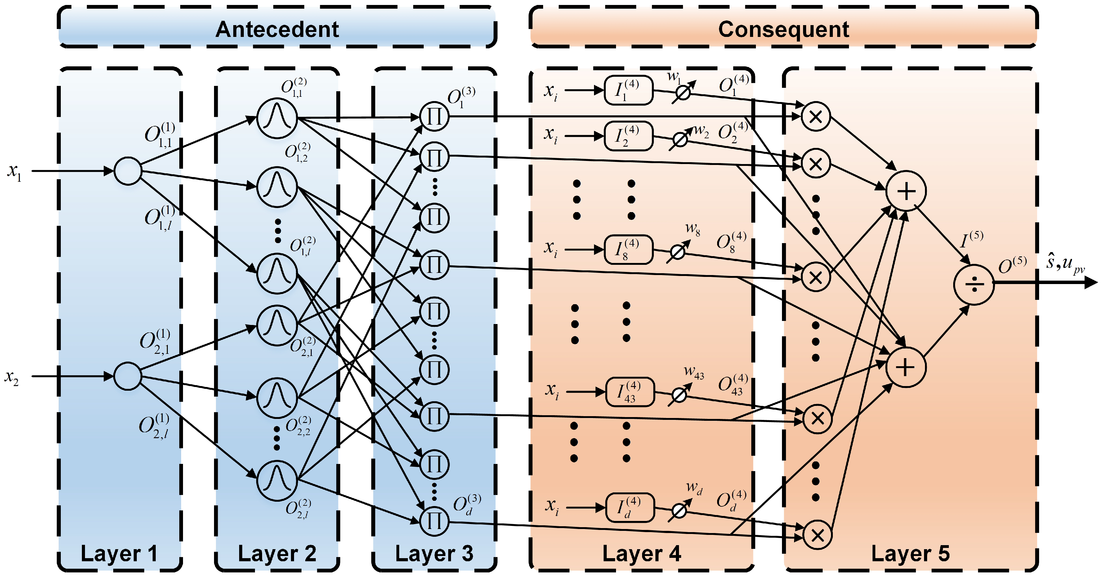
3.1. Structure of the HWANFC and HWNF-Based Gradient Estimator
3.2. Adaptive Mechanism for the HWNF-Based Gradient Estimator
3.3. On-Line Learning Algorithm for HWANFC
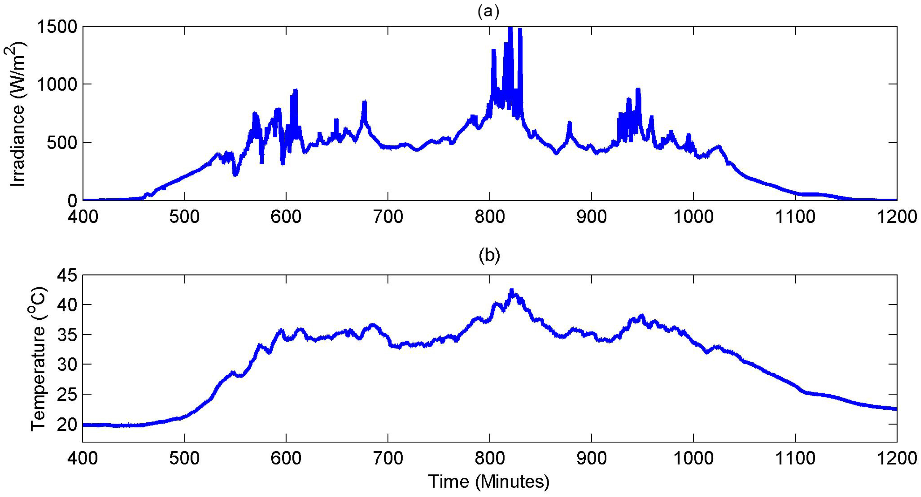
4. Results and Discussion
5. Conclusions
Acknowledgments
Author Contributions
Conflicts of Interest
References
- Skik, N.; Abbou, A. Robust adaptive integral backstepping control for MPPT and UPF of PV system connected to the grid. In Proceedings of the 2016 7th International Renewable Energy Congress (IREC), Hammamet, Tunisia, 22–24 March 2016; pp. 1–6.
- Li, C.H.; Zhu, X.J.; Cao, G.Y.; Hu, W.Q.; Sui, S.; Hu, M.R. A maximum power point tracker for photovoltaic energy systems based on fuzzy neural networks. J. Zhejiang Univ.-Sci. A 2009, 10, 263–270. [Google Scholar] [CrossRef]
- Hassan, S.Z.; Li, H.; Kamal, T.; Nadarajah, M.; Mehmood, F. Fuzzy embedded MPPT modeling and control of PV system in a hybrid power system. In Proceedings of the 2016 International Conference on Emerging Technologies (ICET), Islamabad, Pakistan, 18–19 October 2016; pp. 1–6.
- Xiao, W.; Ozog, N.; Dunford, W.G. Topology study of photovoltaic interface for maximum power point tracking. IEEE Trans. Ind. Electron. 2007, 54, 1696–1704. [Google Scholar] [CrossRef]
- Eltawil, M.A.; Zhao, Z. MPPT techniques for photovoltaic applications. Renew. Sustain. Energy Rev. 2013, 25, 793–813. [Google Scholar] [CrossRef]
- Putri, R.I.; Wibowo, S.; Rifai, M. Maximum power point tracking for photovoltaic using incremental conductance method. Energy Procedia 2015, 68, 22–30. [Google Scholar] [CrossRef]
- Lin, C.H.; Huang, C.H.; Du, Y.C.; Chen, J.L. Maximum photovoltaic power tracking for the PV array using the fractional-order incremental conductance method. Appl. Energy 2011, 88, 4840–4847. [Google Scholar] [CrossRef]
- Li, C.; Chen, Y.; Zhou, D.; Liu, J.; Zeng, J. A high-performance adaptive incremental conductance MPPT algorithm for photovoltaic systems. Energies 2016, 9, 288. [Google Scholar] [CrossRef]
- Raveendhra, D.; Kumar, B.; Mishra, D.; Mankotia, M. Design of FPGA based open circuit voltage MPPT charge controller for solar PV system. In Proceedings of the 2013 International Conference on Circuits, Power and Computing Technologies (ICCPCT), Nagercoil, India, 20–21 March 2013; pp. 523–527.
- Kollimalla, S.K.; Mishra, M.K. A novel adaptive P&O MPPT algorithm considering sudden changes in the irradiance. IEEE Trans. Energy Convers. 2014, 29, 602–610. [Google Scholar]
- Nedumgatt, J.J.; Jayakrishnan, K.B.; Umashankar, S.; Vijayakumar, D.; Kothari, D.P. Perturb and observe MPPT algorithm for solar PV systems-modeling and simulation. In Proceedings of the 2011 Annual IEEE India Conference (INDICON), Hyderabad, India, 16–18 December 2011; pp. 1–6.
- Alajmi, B.N.; Ahmed, K.H.; Finney, S.J.; Williams, B.W. Fuzzy-Logic-Control Approach of a Modified Hill-Climbing Method for Maximum Power Point in Microgrid Standalone Photovoltaic System. IEEE Trans. Power Electron. 2011, 26, 1022–1030. [Google Scholar] [CrossRef]
- Shiau, J.K.; Wei, Y.C.; Chen, B.C. A study on the fuzzy-logic-based solar power MPPT algorithms using different fuzzy input variables. Algorithms 2015, 8, 100–127. [Google Scholar] [CrossRef]
- Ramalu, T.; Mohd Radzi, M.; AtiqiMohd Zainuri, M.; Abdul Wahab, N.; Abdul Rahman, R. A photovoltaic-based SEPIC converter with dual-fuzzy maximum power point tracking for optimal buck and boost operations. Energies 2016, 9, 604. [Google Scholar] [CrossRef]
- Hadjaissa, A.; Ait cheikh, S.M.; Ameur, K.; Essounbouli, N. A GA-based optimization of a fuzzy-based MPPT controller for a photovoltaic pumping system, Case study for Laghouat, Algeria. In Proceedings of the 8th IFAC Conference on Manufacturing Modelling, Management and Control MIM 2016, Troyes, France, 28–30 June 2016; pp. 692–697.
- Salimi, M.; Siami, S. Cascade nonlinear control of DC-DC buck/boost converter using exact feedback linearization. In Proceedings of the 2015 4th International Conference on Electric Power and Energy Conversion Systems (EPECS), Sharjah, UAE, 24–26 November 2015; pp. 1–5.
- Khaldi, N.; Mahmoudi, H.; Zazi, M.; Barradi, Y. The MPPT control of PV system by using neural networks based on Newton Raphson method. In Proceedings of the 2014 International Renewable and Sustainable Energy Conference (IRSEC), Ouarzazate, Morocco, 17–19 October 2014; pp. 19–24.
- Mohapatra, A.; Nayak, B.; Mohanty, K.B. Performance improvement in MPPT of SPV system using NN controller under fast changing environmental condition. In Proceedings of the 2016 IEEE 6th International Conference on Power Systems (ICPS), New Delhi, India, 4–6 March 2016; pp. 1–5.
- Ou, T.C.; Hong, C.M. Dynamic operation and control of microgrid hybrid power systems. Energy 2014, 66, 314–323. [Google Scholar] [CrossRef]
- Hong, C.M.; Ou, T.C.; Lu, K.H. Development of intelligent MPPT (maximum power point tracking) control for a grid-connected hybrid power generation system. Energy 2013, 50, 270–279. [Google Scholar] [CrossRef]
- Ma, S.; Chen, M.; Wu, J.; Huo, W.; Huang, L. Augmented Nonlinear Controller for Maximum Power-Point Tracking with Artificial Neural Network in Grid-Connected Photovoltaic Systems. Energies 2016, 9, 1005. [Google Scholar] [CrossRef]
- Messalti, S.; Harrag, A.; Loukriz, A. A new variable step size neural networks MPPT controller: Review, simulation and hardware implementation. Renew. Sustain. Energy Rev. 2017, 68, 221–233. [Google Scholar] [CrossRef]
- Subiyanto, S.; Mohamed, A.; Hannan, M.A. Intelligent maximum power point tracking for PV system using Hopfield neural network optimized fuzzy logic controller. Energy Build. 2012, 51, 29–38. [Google Scholar] [CrossRef]
- Khosrojerdi, F.; Taheri, S.; Cretu, A.M. An adaptive neuro-fuzzy inference system-based MPPT controller for photovoltaic arrays. In Proceedings of the 2016 IEEE Electrical Power and Energy Conference (EPEC), Ottawa, ON, Canada, 12–14 October 2016; pp. 1–6.
- Abu-Rub, H.; Iqbal, A.; Ahmed, S.M. Adaptive neuro-fuzzy inference system-based maximum power point tracking of solar PV modules for fast varying solar radiations. Int. J. Sustain. Energy 2012, 31, 383–398. [Google Scholar] [CrossRef]
- Rekioua, D.; Achour, A.Y.; Rekioua, T. Tracking power photovoltaic system with sliding mode control strategy. Energy Procedia 2013, 36, 219–230. [Google Scholar] [CrossRef]
- Valencia, P.A.O.; Ramos-Paja, C.A. Sliding-mode controller for maximum power point tracking in grid-connected photovoltaic systems. Energies 2015, 8, 12363–12387. [Google Scholar] [CrossRef]
- Cheng, P.C.; Peng, B.R.; Liu, Y.H.; Cheng, Y.S.; Huang, J.W. Optimization of a fuzzy-logic-control-based MPPT algorithm using the particle swarm optimization technique. Energies 2015, 8, 5338–5360. [Google Scholar] [CrossRef]
- Liu, Y.H.; Liu, C.L.; Huang, J.W.; Chen, J.H. Neural-network-based maximum power point tracking methods for photovoltaic systems operating under fast changing environments. Sol. Energy 2013, 89, 42–53. [Google Scholar] [CrossRef]
- Vazquez, J.R.; Martin, A.D.; Herrera, R.S. Neuro-Fuzzy control of a grid-connected photovoltaic system with power quality improvement. In Proceedings of the 2013 IEEE EUROCON, Zagreb, Croatia, 1–4 July 2013; pp. 850–857.
- Shanthi, T.; Vanmukhil, A.S. ANFIS Controller based MPPT Control of Photovoltaic Generation System. Res. J. Appl. Sci. 2013, 8, 375–382. [Google Scholar]
- Lin, F.J.; Shen, P.H. Adaptive fuzzy-neural-network control for a DSP-based permanent magnet linear synchronous motor servo drive. IEEE Trans. Fuzzy Syst. 2006, 14, 481–495. [Google Scholar]
- Atakulreka, A.; Sutivong, D. Avoiding local minima in feedforward neural networks by simultaneous learning. In Australasian Joint Conference on Artificial Intelligence; Springer: Berlin, Germany, 2007; pp. 100–109. [Google Scholar]
- Choi, B.; Lee, J.H.; Kim, D.H. Solving local minima problem with large number of hidden nodes on two-layered feed-forward artificial neural networks. Neurocomputing 2008, 71, 3640–3643. [Google Scholar] [CrossRef]
- Lo, J.T.H.; Gui, Y.; Peng, Y. Overcoming the Local-Minimum Problem in Training Multilayer Perceptrons with the NRAE Training Method; International Symposium on Neural Networks; Springer: Berlin, Germany, 2012; pp. 440–447. [Google Scholar]
- Lee, C.Y.; Lin, C.J. A wavelet-based neuro-fuzzy system and its applications. Intell. Autom. Soft Comput. 2007, 13, 385–403. [Google Scholar] [CrossRef]
- Abiyev, R.H.; Kaynak, O. Identification and Control of Dynamic Plants Using Fuzzy Wavelet Neural Networks. In Proceedings of the 2008 IEEE International Symposium on Intelligent Control, San Antonio, TX, USA, 3–5 September 2008; pp. 1295–1301.
- Cao, C.; Ma, L.; Xu, Y. Adaptive control theory and applications. J. Control Sci. Eng. 2012, 2012, 827353. [Google Scholar] [CrossRef]
- Rouzbehi, K.; Miranian, A.; Luna, A.; Rodriguez, P. Identification and maximum power point tracking of photovoltaic generation by a local neuro-fuzzy model. In Proceedings of the IECON 2012—38th Annual Conference on IEEE Industrial Electronics Society, Montreal, QC, Canada, 25–28 October 2012; pp. 1019–1024.
- Pradhan, R.; Subudhi, B. Design and real-time implementation of a new auto-tuned adaptive MPPT control for a photovoltaic system. Int. J. Electr. Power Energy Syst. 2015, 64, 792–803. [Google Scholar] [CrossRef]
- Kofinas, P.; Dounis, A.I.; Papadakis, G.; Assimakopoulos, M. An Intelligent MPPT controller based on direct neural control for partially shaded PV system. Energy Build. 2015, 90, 51–64. [Google Scholar] [CrossRef]
- Das, D.; Esmaili, R.; Xu, L.; Nichols, D. An optimal design of a grid connected hybrid wind/photovoltaic/fuel cell system for distributed energy production. In Proceedings of the 31st Annual Conference of IEEE Industrial Electronics Society, IECON 2005, Raleigh, NC, USA, 6–10 November 2005; pp. 2499–2504.
- Xiao, W.; Dunford, W.; Capel, A. A novel modeling method for photovoltaic cells. In Proceedings of the 2004 IEEE 35th Annual Power Electronics Specialists Conference (IEEE Cat. No. 04CH37551), Aachen, Germany, 20–25 June 2004; pp. 1950–1956.
- Kazimierczuk, M.; Starman, L. Dynamic performance of PWM DC-DC boost converter with input voltage feedforward control. IEEE Trans. Circuits Syst. I Fundam. Theory Appl. 1999, 46, 1473–1481. [Google Scholar] [CrossRef]
- Mukerjee, A.; Dasgupta, N. DC power supply used as photovoltaic simulator for testing MPPT algorithms. Renew. Energy 2007, 32, 587–592. [Google Scholar] [CrossRef]
- Gupta, A.; Ray, S.S. An investigation with Hermite Wavelets for accurate solution of Fractional Jaulent–Miodek equation associated with energy-dependent Schrödinger potential. Appl. Math. Comput. 2015, 270, 458–471. [Google Scholar] [CrossRef]
- Ray, S.S.; Gupta, A. A numerical investigation of time-fractional modified Fornberg–Whitham equation for analyzing the behavior of water waves. Appl. Math. Comput. 2015, 266, 135–148. [Google Scholar] [CrossRef]
- Li, C.h.; Zhu, X.j.; Sui, S.; Hu, W.q. Maximum power point tracking of a photovoltaic energy system using neural fuzzy techniques. J. Shanghai Univ. (Engl. Ed.) 2009, 13, 29–36. [Google Scholar] [CrossRef]
- Garcia, P.; Garcia, C.A.; Fernandez, L.M.; Llorens, F.; Jurado, F. ANFIS-Based Control of a Grid-Connected Hybrid System Integrating Renewable Energies, Hydrogen and Batteries. IEEE Trans. Ind. Inform. 2014, 10, 1107–1117. [Google Scholar] [CrossRef]


| LN | MN | SN | ZE | SP | MP | LP | |
|---|---|---|---|---|---|---|---|
| LN | 1.00 () | 1.00 () | 0.66 | 0.66 | 0.33 | 0.33 | 0.00 |
| MN | 1.00 () | 0.66 | 0.66 | 0.33 | 0.33 | 0.00 | −0.33 |
| SN | 0.66 | 0.66 | 0.33 | 0.33 | 0.00 | −0.33 | −0.33 |
| ZE | 0.66 | 0.33 | 0.33 | 0.00 | −0.33 | −0.33 | −0.66 |
| SP | 0.33 | 0.33 | 0.00 | −0.33 | −0.33 | −0.66 | −0.66 |
| MP | 0.33 | 0.00 | −0.33 | −0.33 | −0.66 | −0.66 | −1.00 () |
| LP | 0.00 | −0.33 | −0.33 | −0.66 | −0.66 | −1.00 () | −1.00 () |
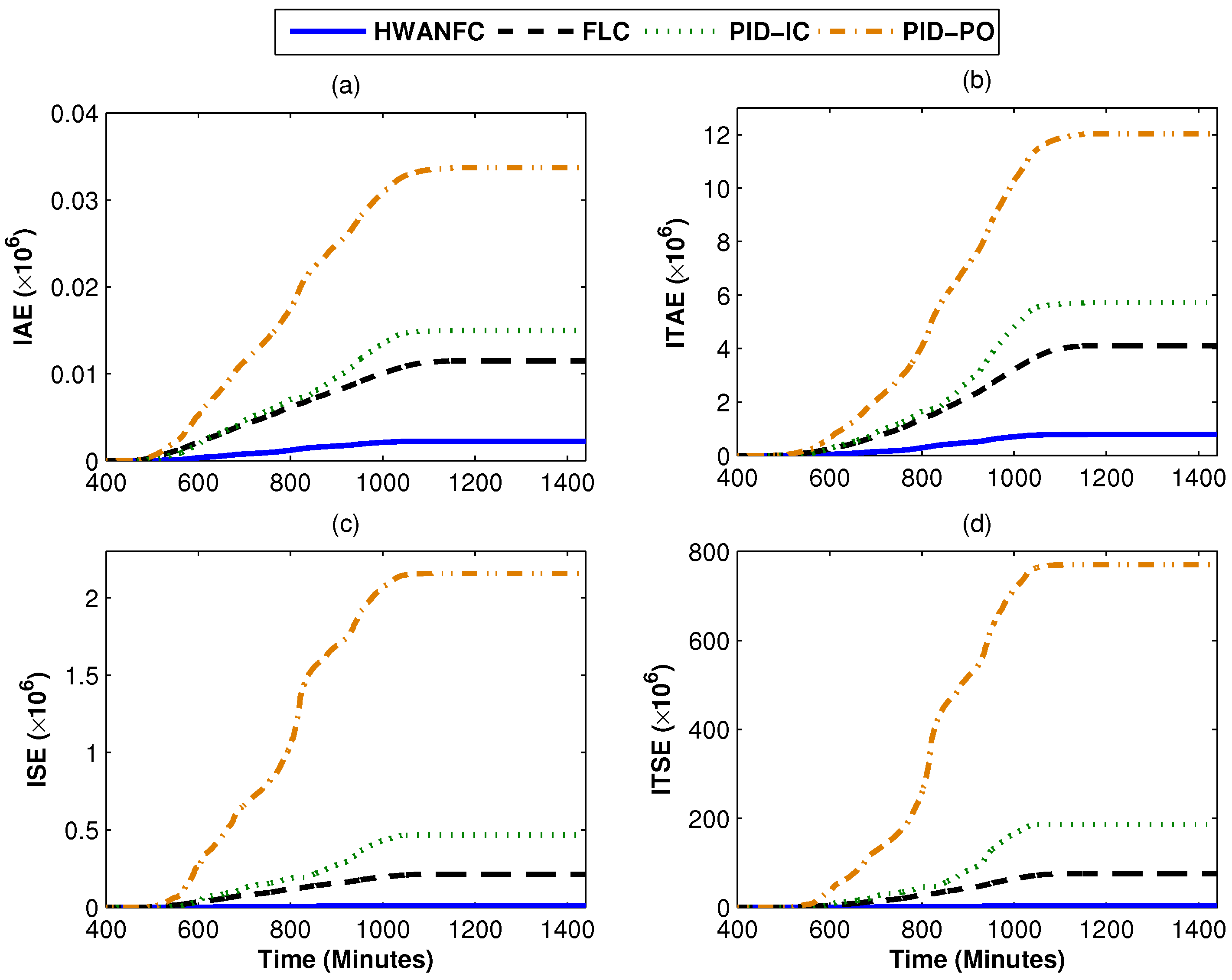
| Controllers | (%age) | (%age) | MRE (103) | IAE (106) | ITAE (106) | ISE (106) | ITSE (106) |
|---|---|---|---|---|---|---|---|
| HWANFC | 96.81 | 94.04 | 0.0029 | 0.00243 | 0.7934 | 0.01043 | 3.666 |
| FLC | 83.66 | 76.63 | 0.0276 | 0.01149 | 4.11 | 0.2146 | 75.66 |
| PID-IC | 80.13 | 75.56 | 3.147 | 0.01498 | 5.72 | 0.4669 | 186.8 |
| PID-P&O | 52.06 | 48.57 | 1.242 | 0.0337 | 12.04 | 2.158 | 770.3 |
© 2017 by the authors. Licensee MDPI, Basel, Switzerland. This article is an open access article distributed under the terms and conditions of the Creative Commons Attribution (CC BY) license ( http://creativecommons.org/licenses/by/4.0/).
Share and Cite
Hassan, S.Z.; Li, H.; Kamal, T.; Arifoğlu, U.; Mumtaz, S.; Khan, L. Neuro-Fuzzy Wavelet Based Adaptive MPPT Algorithm for Photovoltaic Systems. Energies 2017, 10, 394. https://doi.org/10.3390/en10030394
Hassan SZ, Li H, Kamal T, Arifoğlu U, Mumtaz S, Khan L. Neuro-Fuzzy Wavelet Based Adaptive MPPT Algorithm for Photovoltaic Systems. Energies. 2017; 10(3):394. https://doi.org/10.3390/en10030394
Chicago/Turabian StyleHassan, Syed Zulqadar, Hui Li, Tariq Kamal, Uğur Arifoğlu, Sidra Mumtaz, and Laiq Khan. 2017. "Neuro-Fuzzy Wavelet Based Adaptive MPPT Algorithm for Photovoltaic Systems" Energies 10, no. 3: 394. https://doi.org/10.3390/en10030394