
Image Recognition of Icing Thickness on Power Transmission Lines Based on a Least Squares Hough Transform


1
School of Geodesy and Geomatics, Wuhan University, Wuhan 430079, China
2
School of Electrical Engineering, Wuhan University, Wuhan 430072, China
3
School of Mechanical and Electronic Engineering, Wuhan University of Technology, Wuhan 430070, China
*
Authors to whom correspondence should be addressed.
Energies 2017, 10(4), 415; https://doi.org/10.3390/en10040415
Submission received: 13 January 2017
/
Revised: 12 March 2017
/
Accepted: 18 March 2017
/
Published: 23 March 2017
Abstract
:In view of the shortcomings of current image detection methods for icing thickness on power transmission lines, an image measuring method for icing thickness based on remote online monitoring was proposed. In this method, a Canny operator is used to get the image edge, in addition, a Hough transform and least squares are combined to solve the problems of traditional Hough transform in the parameter space whereby it is easily disturbed by the image background and noises, and eventually the edges of iced power transmission lines and un-iced power transmission lines are accurately detected in images which have low contrast, complex grayscale, and many noises. Furthermore, based on the imaging principle of the camera, a new geometric calculation model for icing thickness is established by using the radius of power transmission line as a reference, and automatic calculation of icing thickness is achieved. The results show that proposed image recognition method is rarely disturbed by noises and background, the image recognition results show good agreement with the real edges of iced power transmission lines and un-iced power transmission lines, and is simple and easy to program, which suggests that the method can be used for image recognition and calculation of icing thickness.
1. Introduction
The earliest reports of icing accidents on power transmission lines appeared in 1932, and since then Norway, Canada, Britain, Russia, Japan and other countries or regions have had serious icing disasters. With global abnormal weather occurring frequently in today’s climate, icing disasters on power transmission lines are growing in frequency due to the prevailing macroclimate, micrometeorological, and microtopography conditions. These seriously threaten the safe operation of the power grid and have caused huge losses to the respective national economies.
Power transmission line breakage, transmission tower toppling, ice flashover, power transmission line galloping, etc., caused by icing, often occurred in China during the winter, [1,2,3]. In the 2008 southern snowstorm in China, the direct economic losses of the State Grid and China Southern Power Grid were 10.4 billion and 5 billion RMB, and the indirect economic losses and social impact caused by the power outage were more difficult to estimate [4,5,6]. In order to ensure the normal operation of the power system, reduce and prevent icing disaster consequences on power transmission lines, it is necessary achieve real-time online monitoring of icing thickness on these lines.
Compared with weighing methods which are susceptible to wind and magnetic fields, icing rate meter methods which cannot directly measure icing thickness on power transmission lines, optical fiber sensing methods which have characteristics of zero drift and non-linearity, and wire dip methods which are susceptible to stiffness on rotating power transmission lines, image recognition methods which are real-time and visible have been a recent trend and direction of research on icing monitoring methods.
In the current world, the vast majority of transmission towers are equipped with remote online monitoring terminals, and these could collect and transfer real-time icing images to monitoring centers, so we can obtain the real-time icing status from icing images, and then calculate the icing thickness to further assess the icing harm potential on power transmission lines. However, the background environment of power transmission lines is complex, the imaging environment is easily affected by light factors, and lossy compression methods are applied to the image transmission process, which leads to icing images having characteristics of low contrast, complex grayscale, all kinds of noises, etc. [7,8]. At present, image recognition algorithms for icing thickness on power transmission lines rarely take into account these aspects. For example, based on obtaining all slopes of the power transmission line in an image, the slope line searching algorithm described in [9] calculates the mainstream slope as the edge of the iced power transmission line. In this method, some slopes which do not belong to the power transmission line will affect the calculation of the mainstream slope. In addition, the optimal threshold and mathematical morphology algorithm from [10] can only get the edges of the iced power transmission line from images which have simple backgrounds. In fact, power transmission line icing images have very complex backgrounds. Similarly, the automatic tracking algorithm from [11] simply averages the vertical coordinates of the upper outline pixels and lower outline pixels of the iced power transmission line, without considering the impacts of image noises.
To address the above problems, this paper presents an image recognition algorithm for icing thickness on power transmission linea based on a least squares Hough transform. Compared with the shortcomings of the traditional Hough transform which is easily affected by background and noises in parameter space [12,13,14,15], this algorithm combines a Hough transform with the least squares method, and then accurately identifies the edges of iced power transmission lines and un-iced power transmission lines in images which have low contrast, complex grayscale, and many noises. In addition, a new geometric model of icing thickness was established to automatically calculate icing thickness. An engineering example was carried out to test and verify this proposed image recognition method.
2. Image Recognition Process
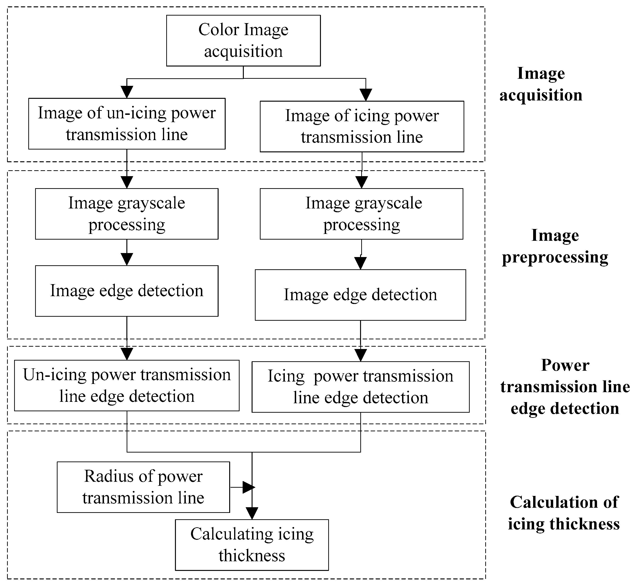
Based on the least squares Hough transform, this paper presents an image recognition algorithm for icing thickness on power transmission line, which can be divided into four steps: image acquisition, image preprocessing, power transmission line edge detection, and calculation of icing thickness. The specific implementation process is as shown in Figure 1 and involves the following steps:
- The color images of un-iced and iced power transmission lines should be respectively subjected to grayscale processing to obtain grayscale images. After that, the Canny operator is used to detect the edges of the two images. By setting a self-adaptation dual threshold in the Canny operator, the edges of un-iced power transmission lines and iced power transmission line are preserved to a certain extent and then non-edge pixels are removed to the greatest degree.
- In the edges of the two images, a Hough transform is used to search for the pixels located on a straight line, and then achieve a rough positioning of the un-iced and iced power transmission line edges. At the same time, least squares fitting is applied to the pixel coordinates of the rough positioning based on the linear equation, and we can get accurate un-iced and iced power transmission line edges. Finally, the pixel coordinate equations of the power transmission line edges are obtained.
- Based on the imaging principle of the camera and the power transmission line edge detection results, a geometrical calculation model for icing thickness is established with reference to the radius of the power transmission line. Then we can achieve automatic calculation of icing thickness.
3. Image Preprocessing
The color images are taken using a remote camera mounted on the tower, and then a lossy compression method is applied to the image transmission process, so these images have complex backgrounds, low contrast, and many kinds of noises, which affect the edge detection of power transmission lines, therefore, the purposes of image preprocessing in this paper are to eliminate image noises, improve image contrast, obtain image edges, and make appropriate preparations for power transmission line edge detection.
3.1. Grayscale Processing
Conversion formulas from color image to grayscale image are as follows:
where P is the pixel in image, R is the red component, G is the green component, and B is the blue component. Based on grayscale processing, the grayscale images shown in Figure 3 are obtained.
3.2. Image Edge Detection
The Canny operator is the most effective edge detection algorithm, whose process can be divided into four steps: Gaussian filtering, gradient calculation, non-maximum suppression, and dual threshold edge detection.
3.2.1. Gaussian Filtering
We use a remote camera mounted on the tower to take images, so the imaging environment is easily affected by the light intensity, light uniformity and other factors, thus Gaussian noises are easily produced in images and affect image edge detection. However, Gaussian noises can be eliminated by Gaussian filtering. The weighted average gray value of target pixel and neighborhood pixels is re-assigned to gray value of the target pixel, that is, the image is scanned with the 3 × 3 template (refer to (2)), and the weighted average gray value is re-assigned to the gray value of the center pixel:
3.2.2. Gradient Calculation
On the edges of the image, the gray values of adjacent pixels obviously change. Therefore, the core problem of image edge detection is to find the pixels with “jumping” gray value. In the digital image processing and analysis process, amplitude and direction of the gradient are calculated by the finite difference of the first-order partial derivative, which are used to describe the degree and direction of the pixel gray value changes, and then determine the image edges.
Gaussian filtering can’t remove all the image noises. To further eliminate the effects of image noises on edge detection, a Sobel template operator is used for the convolution calculation:
where P is the pixel matrix of image, (Gx, Gy) is a gradient vector.
Then the gradient amplitude G and direction O are also obtained by (4):
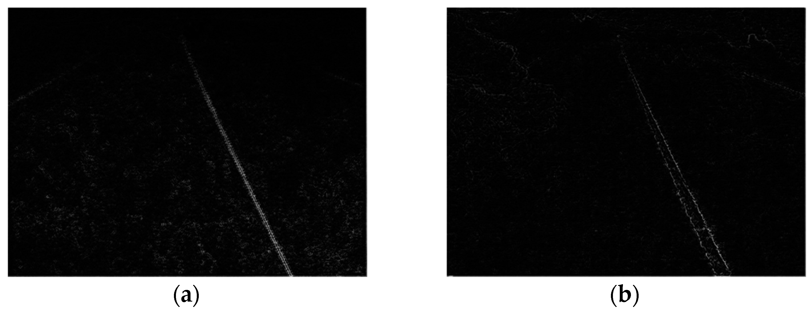
Based on , we assign the gradient amplitude Gi directly to the pixel gray value Pi.g by scaling, where Gmax is the maximum value of image gradient amplitude. Then the grayscale images of gradient amplitude are obtained. As shown in Figure 5, using the gradient amplitude G as the image edge directly can improve the image contrast and enhance the edge features of the image, but not enough to determine the edges of the image.
3.2.3. Non-Maximum Suppression
A number of non-edge pixels are included in Figure 5, so we can eliminate pixels with small gradient values and preserve pixels with local largest gradient values to eliminate non-edge pixels. That method is non-maximum suppression. Non-maximum suppression is performed in the gradient direction, and the pixels where the local gradient amplitude is the largest are retained. In order to simplify the comparison of the gradient amplitude, the gradient angle O needs to be processed as follows:
Step 1: The range of inverse trigonometric function is , so the gradient angle O obtained by (4) can plus a constant , and then range becomes .
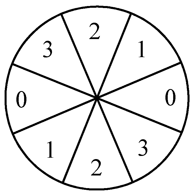
Step 2: Based on Table 1 and Figure 6, the gradient angles O are divided into four sectors of the circumference, and then the gradient angles O are reset.
Based on the gradient angle O of each pixel after resetting, we traverse two adjacent pixels in the gradient direction and then compare the gradient amplitude G: If the gradient amplitude of the target pixel is greater than the gradient amplitudes of the adjacent two pixels, the gradient amplitude of the target pixel is the maximum value, and then its gradient amplitude is scaled by (5). Otherwise, the gradient amplitude of target pixel will be reset to zero:
where Gmax is the maximum value of the image gradient amplitude and Gi is gradient amplitude of target pixel. After the non-maximum suppression, the gradient amplitudes G have been a certain degree of shrinkage. Meanwhile, the pixels with the largest local gradient amplitude are retained, whose gradient amplitudes are scaled to their gray values, and then gray values of other pixels are reset to zero, as shown in Figure 7.
3.2.4. Dual Threshold Edge Detection
The purpose of image edge detection in this paper is to better identify the edges of un-iced power transmission lines and iced power transmission lines, which tries to keep the image foreground and remove the image background. However, the purpose of the traditional Canny operator for image edge detection is to obtain the optimal image edges, which does not consider removing image background.
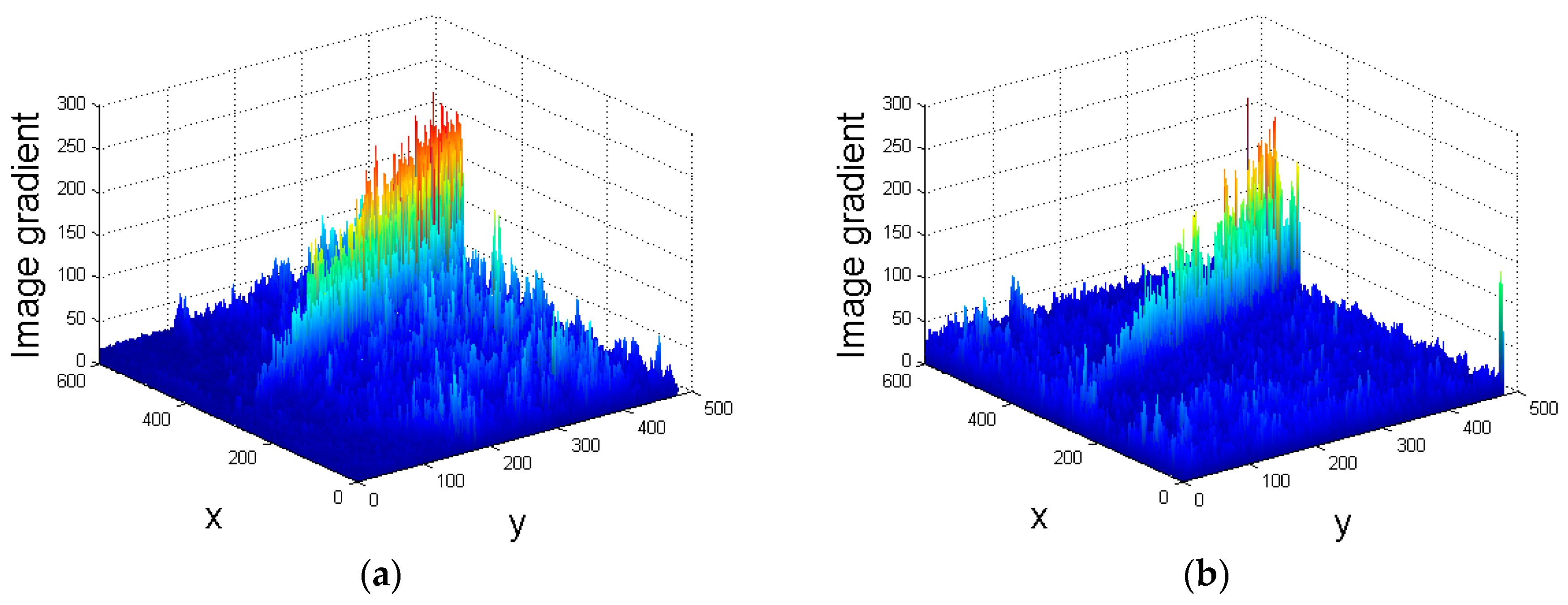
In order to retain power transmission line edges and remove non-power transmission line edges, we can set a dynamic dual threshold based on the gradient amplitude of the power transmission line edges. The high threshold H is the very obvious gradient amplitude of power transmission line edges, and then the low threshold L is gradient demarcation point of power transmission line edges and non-power transmission line edges. When Gi > H, we think that the target pixel must be the image edge. When Gi < L, we think that the target pixel must not be image edge. The pixel whose gradient amplitude is between L and H is further verified as the pending image edge: If the gradient amplitude of pixel is smaller than the high threshold value H in the range of 3 × 3 neighborhood, the pixel is not the image edge. In final obtained image edges, power transmission line edges are preserved to a certain extent and then non-power transmission line edges are removed on the greatest degree. The three-dimensional display image of the gradient amplitude (or gray value) of Figure 7 is obtained as shown in Figure 8.
As can be seen from Figure 8, the gradient amplitudes of the pixels only change significantly at the edge of the power transmission line and reach a peak value; what’s more, the changes in other locations are small.
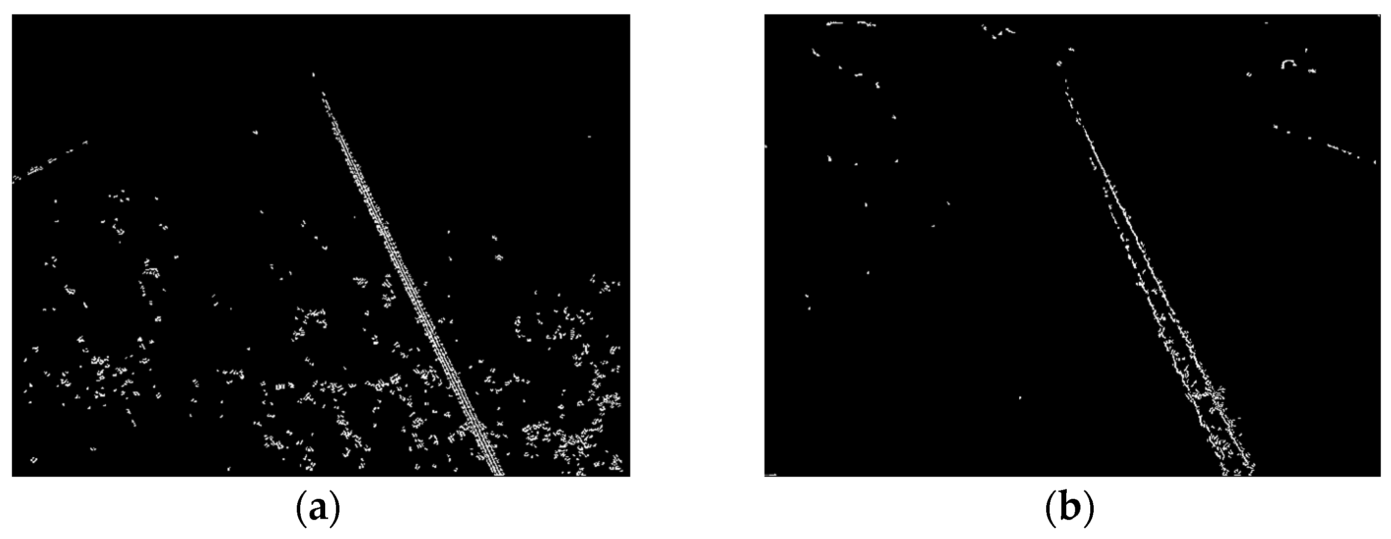
Moreover, it is observed that pixels with gradient amplitude greater than 50 in Figure 8 are substantially located at the edge of the power transmission line, and then parts of pixels with gradient amplitude greater than 25 are also located at the edges, so the high threshold value of Figure 8a,b can be 50, and then the low threshold value of Figure 8a,b can be 25. Based on dual threshold, we further determine the image edges. Finallly, after determining the image edges, we set the gray values of the edge pixels to 255 and the gray values of the non-edge pixels to 0 to get the binary edges of image, as shown in Figure 9. As can be seen from this figure, while carrying on the edge detection, we have retained the edges of the power transmission line to the greatest extent possible, and removed some non-edges of power transmission line.
4. Power Transmission Line Edge Detection Based on Least Squares Hough Transform
In order to further identify the edges of the power transmission line from the image edges, this paper presents a new algorithm based on a least squares Hough transform. The Hough transform is used to locate the edges of un-iced power transmission lines and iced power transmission lines roughly, and then the least squares method is used to locate them accurately.
4.1. Rough Positioning
The principle of the Hough transform is to transform the straight line detection problem of image space into parameter space by using the mapping relation between image space and parameter space. Then we determine the pixels located on the same line by finding the cumulative peak in the parameter space [17,18,19,20,21,22,23]. Therefore, the Hough transform can be used for rough positioning of un-iced power transmission line edge and iced power transmission line edge.
In the image space i-j, all collinear points can be represented by a straight line equation:
where k is the slope of the straight line and b is the intercept.
Taking (i, j) as the parameter, and (k, b) as the variable, we can get (7):
where i is the slope of the straight line and j is the intercept. So (7) can be regarded as a linear equation of parameter space k-b.
Thus, a point in the image space corresponds to a straight line in the parameter space, and points collinear in the image space intersect at the same point in the parameter space, as shown in Figure 10.
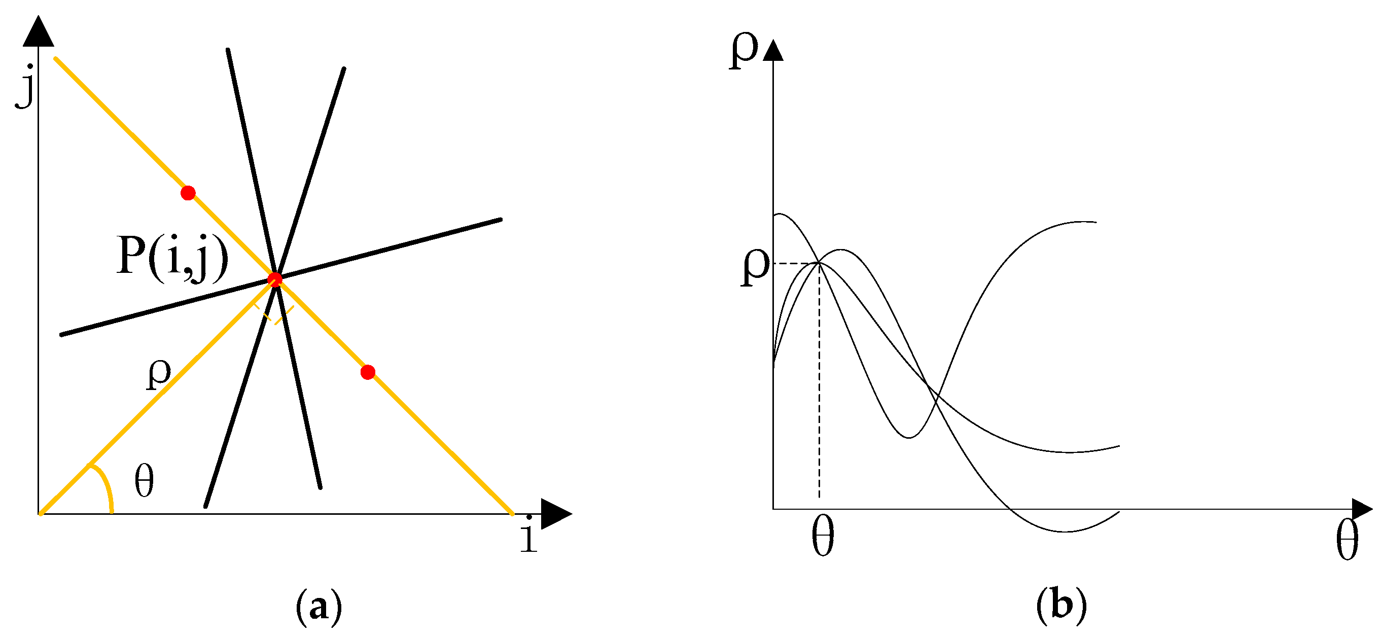
If the slope of straight line in the image space is infinite (the linear equation x = a), the above corresponding relationship will not be expressed. In order to be able to express any slopes of straight line detection, the parameter coordinate (k, b) should be expressed as polar coordinates (, ):
where is the distance from coordinate origin to the straight line, and is the angle between the vertical line passing through the origin and the positive direction of i axis.
We assume straight lines of n directions for each pixel point P(i, j), (n = 180, the angular accuracy of the detection line is 1°) and then calculate the (, ) coordinates of the n straight lines separately, as shown in Figure 11. Finally, we can get the corresponding polar coordinates of n straight lines of all pixel points. Therefore, a point in the image space corresponds to a sinusoidal curve in the parameter space, while collinear points in the image space intersect at the same point in the parameter space.
Based on the mapping relationship between the image space i-j and the parameter space -, we detect the pixels of image edges in Figure 9, and then calculate under all , at the same time, accumulate the occurrence number of under . The results are shown in Figure 12.
When the cumulative number is greater than the threshold value PL, the pixels are on a straight line whose pixel length is greater than threshold value PL. In order to accurately detect the edges on both sides of the power transmission line, the selected threshold PL should be significantly larger than the cumulative number of the other non-edge lines. By observing Figure 12, the occurrence number of under in power transmission line edges is significantly larger than non-edge lines, so the optimum threshold can be chosen as 100.
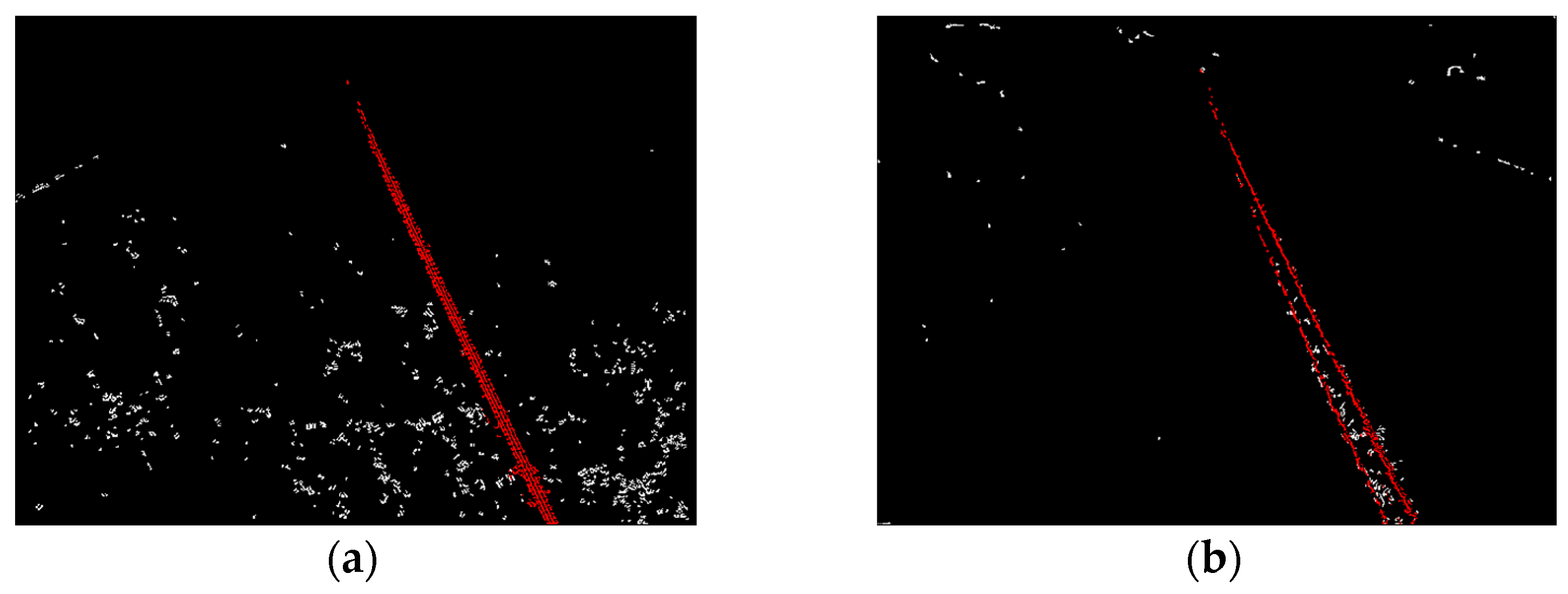
We set the color of detected power transmission line edge pixels to red by setting PL = 100. The rough positioning results of the power transmission line edge after Hough transform are shown in Figure 13 with the red color pixels.
4.2. Accurate Positioning
The power transmission line edge pixels detected by the Hough transform may be located on a a number of straight lines whose pixel length are greater than PL, because the Hough transform is easily affected by image background and noises. In order to obtain the optimal single pixel power transmission line edges from power transmission line edges, it is necessary to carry out a pixel coordinate fitting of the power transmission line edges by the least square function.
First of all, we can determine the center pixel coordinate equation of the power transmission line to split the power transmission line pixels of both sides. Based on (6), the coordinates of all power transmission line edge pixels are regressed by least squares to calculate center pixel coordinate equation of the power transmission line is calculated:
Secondly, the pixels of power transmission line edges are divided into two groups based on (10):
Each group of pixels is located on one side of the power transmission line. Once again, the least square fitting is performed using (6) for each group of pixel coordinates to obtain the optimal single pixel edge on both sides of power transmission line:
Finally, the grayscale value of pixels obtained by the optimal edge is set to 255, that is, the pixel color is set to white, so we can obtain the accurate positioning results of power transmission line edge. Based on rough power transmission line edges (see Figure 13), we can get pixel coordinate equations of optimal edges on both sides of the power transmission line after accurate positioning:
The optimal single pixel edges of power transmission line are as shown in Figure 14. As shown in Figure 14, the edge detection algorithm based on the least squares Hough transform is less sensitive to non-edge pixels and image noises, and then can accurately identify the edges of un-iced power transmission line and iced power transmission line in images with complicated background and various noises.
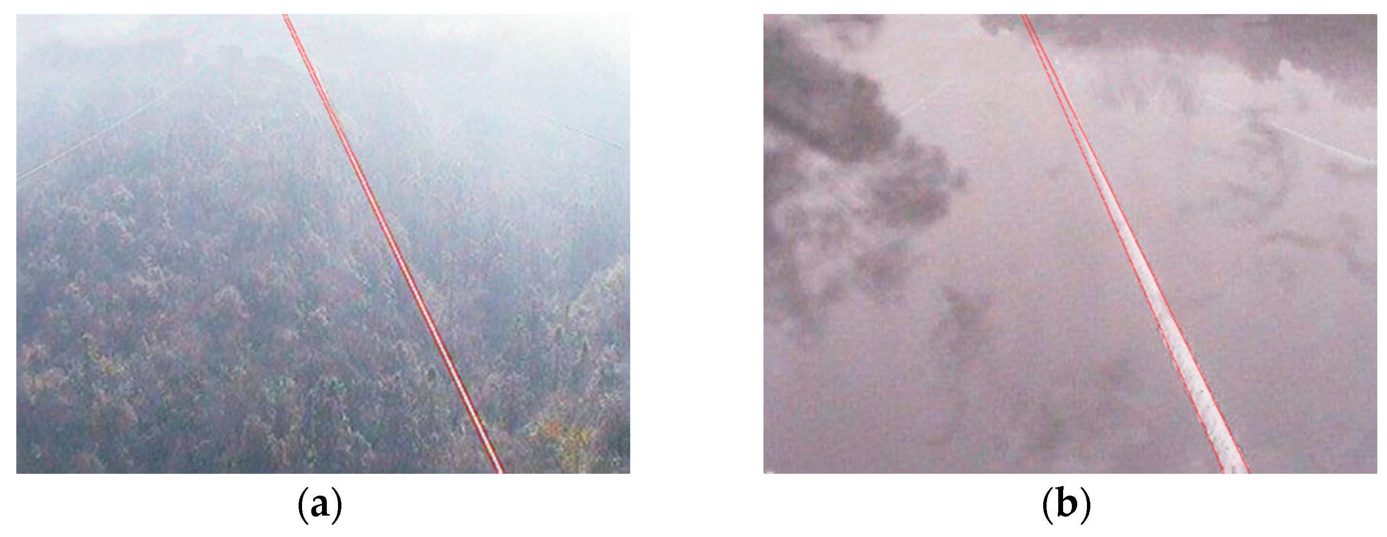
We place accurate positioning results of power transmission line edge into the original color images, as shown in Figure 15 with the red color pixels. Accurate positioning results of the power transmission line edge have a good agreement with the edges of the un-iced power transmission line and iced power transmission line in the original color images.
5. Calculation of Icing Thickness
5.1. Calculating Icing Thickness Based on the Least Squares Hough Transform
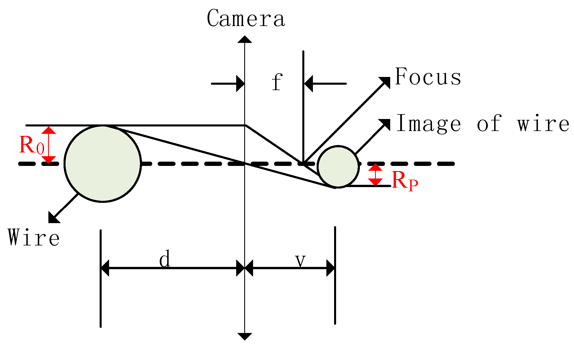
The imaging principle of the camera is as shown in Figure 16. The camera can be seen as a convex lens, f is the focal length, d is the object distance, and v is the image distance.
Based on the imaging principle of convex lens, we can get (14):
where Rp is the size of the image, and R0 is the radius of power transmission line.
We use a remote camera mounted at a fixed position on the tower to take images of un-iced power transmission lines and iced power transmission lines at a fixed angle. Therefore, the deformation ratio is fixed and the same at the same position of the image. Then we can get the calculation formula of icing thickness based on the images of un-iced power transmission lines and the images of iced power transmission lines.
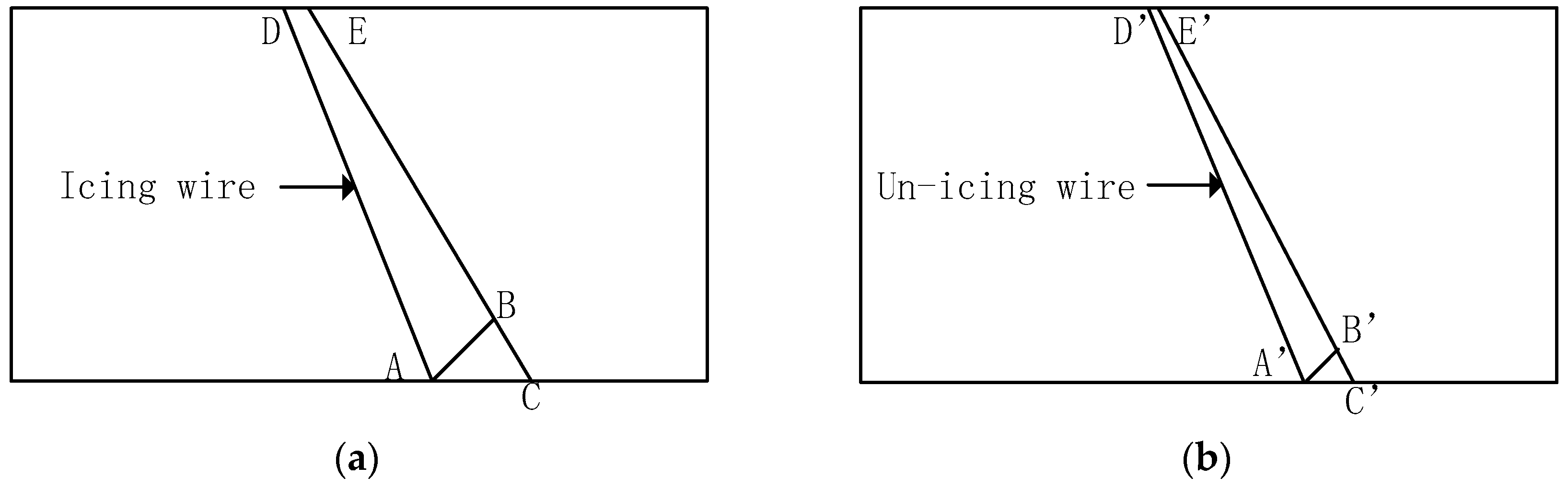
where D is icing thickness, x2 is the pixel radius of the icing power transmission line and x1 is the pixel radius of un-icing power transmission line. To get x2/x1, we need to do the following analysis:
At point A of Figure 17a, the pixel radius of the iced wire is AB/2. Likewise, A’B’/2 is the pixel radius of the un-iced wire (see Figure 17b). The camera takes images from a fixed position and at a fixed angle, so ΔABC and ΔA’B’C’ are similar, then:
So the geometrical calculation model of icing thickness on power transmission line is obtained:
According to edge detection results of the power transmission line (Equations (12) and (13)), we substitute the image pixel height into equation unknown number j, and then get A’C’ = 8.46 pixel and AC = 27.21 pixel.
Compared with the manual count results of power transmission line edge on original image, the recognition error is <1 pixel, as shown in Table 2.
Therefore, the image recognition algorithm based on least squares Hough transform can accurately detect power transmission line edge. The known power transmission line is ACSJ-400/50, whose diameter is 27.63 mm, so the icing thickness D = 30.62 mm can be calculated by Equation (17).
5.2. Comparison with Other Image Recognition Methods
Although we do not know the real icing thickness on the monitoring point, the real average icing thickness of the entire power transmission line is 21.22 mm, so the average icing thickness of the entire power transmission line can be used as a reference for the icing thickness at the monitoring point to verify its correctness. We tested other image recognition methods in Figure 2 and calculate the icing thickness. The final results are shown in Table 3.
As can be seen from Table 3, the error of method D is the largest in the calculated icing thickness results. In this method, we have used 10 sets of two random points on the power transmission line edges to calculate the icing thickness. The resulting icing thickness, which ranges from 17.97 mm to 57.47 mm, depends on the accuracy of the two random points and then produces very unstable results. Method C uses the maximum distance of the power transmission line edges to calculate icing thickness, so the resulting error is the largest of methods A, B and C. Obviously, the calculated icing thickness from method A and method B are closest to the real icing thickness. Compared with method A, method B accumulates all the pixel coordinates to compute an average, which can require a large amount of calculation. In summary, the image recognition algorithm based on least squares Hough transform can accurately detect and calculate icing thickness. Moreover, it’s an easy and stable algorithm.
6. Conclusions
Aiming at the shortcomings of current icing thickness detection methods for power transmission lines, a new image recognition method for icing thickness on power transmission lines based on a least squares Hough transform is proposed in this paper.
Firstly, the grayscale images of un-iced power transmission lines and iced power transmission lines are obtained by grayscale processing. Secondly, according to the principle of preserving power transmission line edges and removing non-edges, we set the self-adaptation dual threshold based on image gradient change and then detect the image edges by a Canny operator. Thirdly, the Hough transform is combined with the least squares method to accurately detect power transmission line edges and get pixel coordinate equations of optimal single pixel edges. Finally, according to the imaging principle of the camera and the real radius of the un-iced power transmission line, the geometric calculation model for icing thickness is established to achieve automatic calculation of icing thickness.
The algorithm can be used to accurately extract power transmission line edges in the images with complex backgrounds and noise interference. It solves the shortcomings of the traditional Hough transform in the parameter space which is easy to be disturbed by the image background and noises, and then realizes the automatic calculation of icing thickness. Therefore, this paper explores a new approach to image recognition of icing thickness. It is proved that the method is sensitive to image background and noises, and identification errors of power transmission line edges are less than 1 pixel. Furthermore, this method is simple and easy to program, and has a certain practicality.
Acknowledgments
This work was supported in part by the National Natural Science Foundation of China (Grant Number 51507114) and in part by the National Natural Science Foundation of China (Grant Number 51507122).
Author Contributions
All authors conceived and designed the study. Under the guidance of Junhua Wang and Jiangui Li, Jingjing Wang implemented the methodology with the assist of Jianwei Shao. Jingjing Wang, Junhua Wang and Jiangui Li wrote the document, and all authors read and approved the final manuscript.
Conflicts of Interest
The authors declare no conflict of interest.
References
- Jiang, X.; Xiang, Z.; Zhang, Z.; Hu, J.; Hu, Q.; Shu, L. Predictive model for equivalent ice thickness load on overhead transmission lines based on measured insulator string deviations. IEEE Trans. Power Deliv. 2014, 29, 1659–1665. [Google Scholar] [CrossRef]
- Hu, J.; Sun, C.; Jiang, X.; Xiao, D.; Zhang, Z.; Shu, L. DC flashover performance of various types of ice-covered insulator strings under low air pressure. Energies 2012, 5, 1554–1576. [Google Scholar] [CrossRef]
- Hu, J.; Sun, C.; Jiang, X.; Yang, Q.; Zhang, Z.; Shu, L. Model for predicting DC flashover voltage of pre-contaminated and ice-covered long insulator strings under low air pressure. Energies 2011, 4, 628–643. [Google Scholar] [CrossRef]
- Hu, J.; Jiang, X.; Yin, F.; Zhang, Z. DC flashover performance of ice-covered composite insulators with parallel air gaps. Energies 2015, 8, 4983–4999. [Google Scholar] [CrossRef]
- Ma, T.; Niu, D. Icing forecasting of high voltage transmission line using weighted least square support vector machine with fireworks algorithm for feature selection. Appl. Sci. 2016, 6, 438. [Google Scholar] [CrossRef]
- Hou, H.; Yin, X.; You, D.; Chen, Q.; Tong, G.; Zheng, Y.; Shao, D. Analysis of the defects of power equipment in the 2008 snow disaster in southern China area. High Volt. Eng. 2009, 35, 584–590. [Google Scholar]
- Xin, G.; Jin, X.; Hu, X. On-line monitoring system of transmission line icing based on DSP. In Proceedings of the 2010 the 5th IEEE Conference on Industrial Electronics and Applications (ICIEA), Taichung, Taiwan, 15–17 June 2010; pp. 186–190. [Google Scholar]
- Qi, L.; Wang, J.; Chen, Y. Research on the image segmentation of icing line based on NSCT and 2-D OSTU. In Proceedings of the 2015 7th International Conference on Modelling, Identification and Control, Sousse, Tunisia, 18–20 December 2015; pp. 1–5. [Google Scholar]
- Lu, J.; Lo, J.; Zhang, H.; Li, B. An Image recognition algorithm based on thickness of ice cover of transmission line. In Proceedings of the 2011 International Conference on Image Analysis and Signal Processing (IASP), Wuhan, China, 21–23 October 2011; pp. 210–213. [Google Scholar]
- Wang, X.; Hu, J.; Wu, B.; Du, L.; Sun, C. Study on edge extraction methods for image-based icing on-line monitoring on overhead transmission lines. In Proceedings of the 2008 International Conference on High Voltage Engineering and Application, Chongqing, China, 9–13 November 2008; pp. 9–13. [Google Scholar]
- Zhong, Y.; Zuo, Q.; Zhou, Y.; Zhang, C. A new image-based algorithm for icing detection and icing thickness estimation for transmission lines. In Proceedings of the IEEE International Conference on Multimedia and Expo Workshops, San Jose, CA, USA, 15–19 July 2013; pp. 1–6. [Google Scholar]
- Shi, D.; Zheng, L.; Liu, J. Advanced hough transform using a multilayer fractional fourier method. IEEE Trans. Image Process. 2010, 19, 1558–1566. [Google Scholar] [PubMed]
- Li, W.; Cui, X.; Guo, L.; Chen, J.; Chen, X.; Cao, X. Tree root automatic recognition in ground penetrating radar profiles based on randomized hough transform. Remote Sens. 2016, 8, 430. [Google Scholar] [CrossRef]
- Díaz-Vilariño, L.; Conde, B.; Lagüela, S.; Lorenzo, H. Automatic detection and segmentation of columns in as-built buildings from point clouds. Remote Sens. 2015, 7, 15651–15667. [Google Scholar] [CrossRef]
- Lu, X.; Song, L.; Shen, S.; He, K.; Yu, S.; Ling, N. Parallel hough transform-based straight line detection and its FPGA implementation in embedded vision. Sensors 2013, 13, 9223–9247. [Google Scholar] [CrossRef] [PubMed]
- Hao, Y.; Liu, G.; Xue, Y.; Zhu, J.; Shi, Z.; Li, L. Wavelet image recognition of ice thickness on transmission lines. High Volt. Eng. 2014, 40, 368–373. [Google Scholar]
- Ho, C.G.; Young, R.C.D.; Bradfield, C.D.; Chatwin, C.R. A fast hough transform for the parametrisation of straight lines using fourier methods. Real-Time Imaging 2000, 6, 113–127. [Google Scholar] [CrossRef]
- Duda, R.O.; Hart, P.E. Use of the Hough transformation to detect lines and curves in pictures. Commun. ACM 1972, 15, 11–15. [Google Scholar] [CrossRef]
- Xu, L.; Oja, E.; Kultanen, P. A new curve detection method randomized Hough transform (RHT). Pattern Recognit. Lett. 1990, 11, 331–338. [Google Scholar] [CrossRef]
- Xu, L.; Oja, E. Randomized hough transform (RHT): Basic mechanisms, algorithms, and complexities. CVGIP Image Underst. 1993, 57, 131–154. [Google Scholar] [CrossRef]
- Du, S.Z.; Tu, C.L.; van Wyk, B.J.; Chen, Z.Q. Collinear segment detection using HT neighborhoods. IEEE Trans. Image Process. 2011, 20, 3612–3620. [Google Scholar] [PubMed]
- Ballard, D.H. Generalizing the Hough transform to detect arbitrary shapes. Pattern Recogn. 1981, 13, 111–122. [Google Scholar] [CrossRef]
- Rau, J.Y.; Chen, L.C. Fast straight line detection using Hough transform with principal axis analysis. J. Photogramm. Remote Sens. 2003, 8, 15–34. [Google Scholar]
- Huang, X.; Wei, X. A New on-line monitoring technology of transmission line conductor icing. In Proceedings of the International Conference on Condition Monitoring and Diagnosis, Bali, Indonesia, 23–27 September 2012; pp. 581–585. [Google Scholar]
- Li, Z.X.; Hao, Y.P.; Li, L.C.; Yang, L.; Fu, C. Image recognition of ice thickness on transmission lines using remote system. High Volt. Eng. 2011, 37, 2288–2293. [Google Scholar]
Figure 1.
The image recognition process for icing thickness on power transmission lines.

Figure 2.
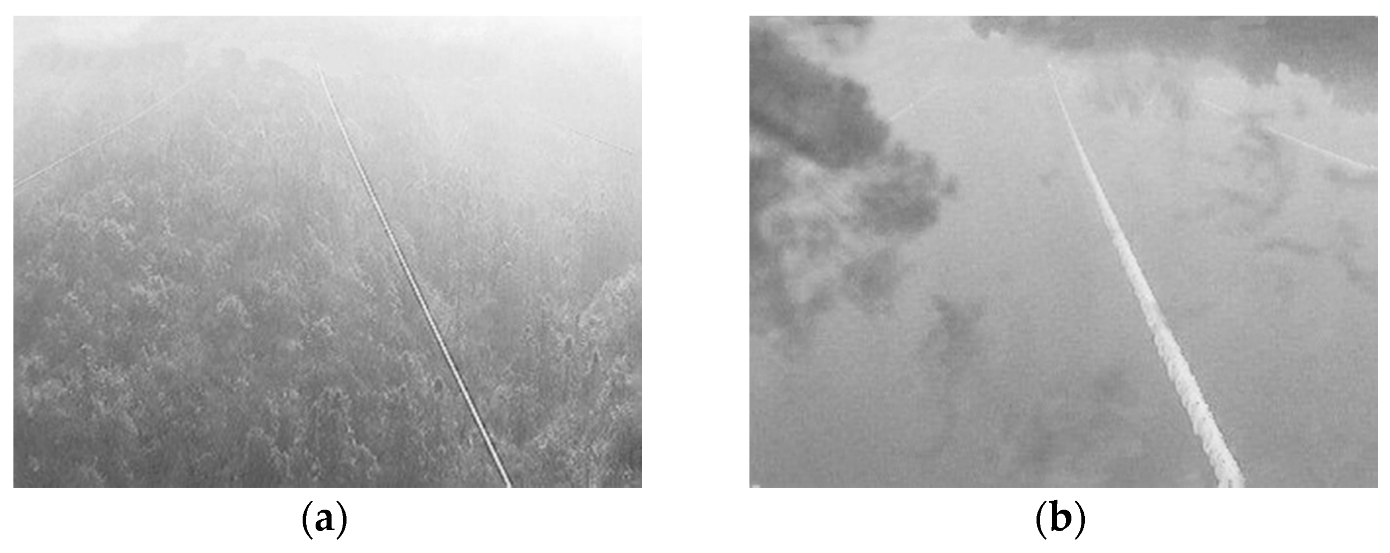
The color images are captured from a fixed remote camera, whose image size is 640*480. (a) A color image of an un-iced power transmission line; (b) A color image of an iced power transmission line.
Figure 2.
The color images are captured from a fixed remote camera, whose image size is 640*480. (a) A color image of an un-iced power transmission line; (b) A color image of an iced power transmission line.

Figure 3.
The grayscale images of Figure 2. (a) A grayscale image of an un-iced power transmission line; (b) A grayscale image of an iced power transmission line.
Figure 3.
The grayscale images of Figure 2. (a) A grayscale image of an un-iced power transmission line; (b) A grayscale image of an iced power transmission line.

Figure 4.
Grayscale images after Gaussian filtering. (a) A grayscale image of an un-iced power transmission line after Gaussian filtering; (b) A grayscale image of an iced power transmission line after Gaussian filtering.
Figure 4.
Grayscale images after Gaussian filtering. (a) A grayscale image of an un-iced power transmission line after Gaussian filtering; (b) A grayscale image of an iced power transmission line after Gaussian filtering.
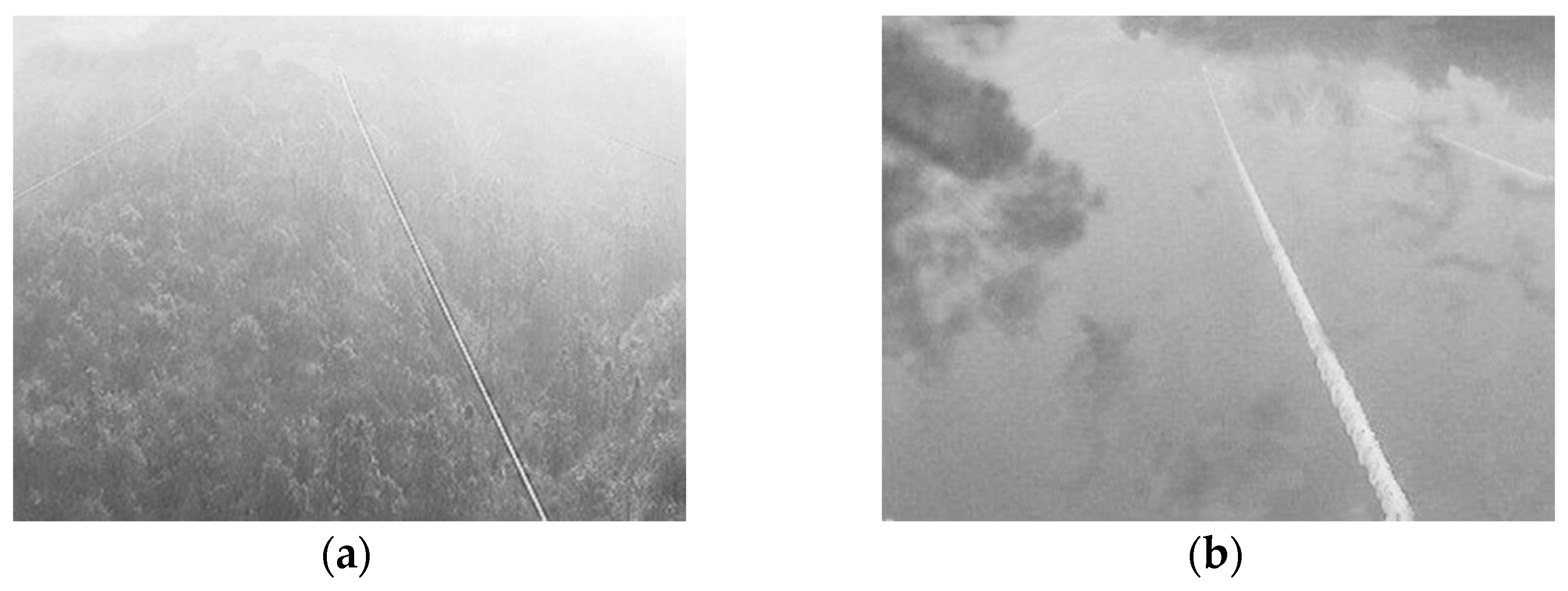
Figure 5.
The grayscale images based on gradient amplitude. (a) Gradient image of an un-iced power transmission line; (b) Gradient image of an iced power transmission line.
Figure 5.
The grayscale images based on gradient amplitude. (a) Gradient image of an un-iced power transmission line; (b) Gradient image of an iced power transmission line.
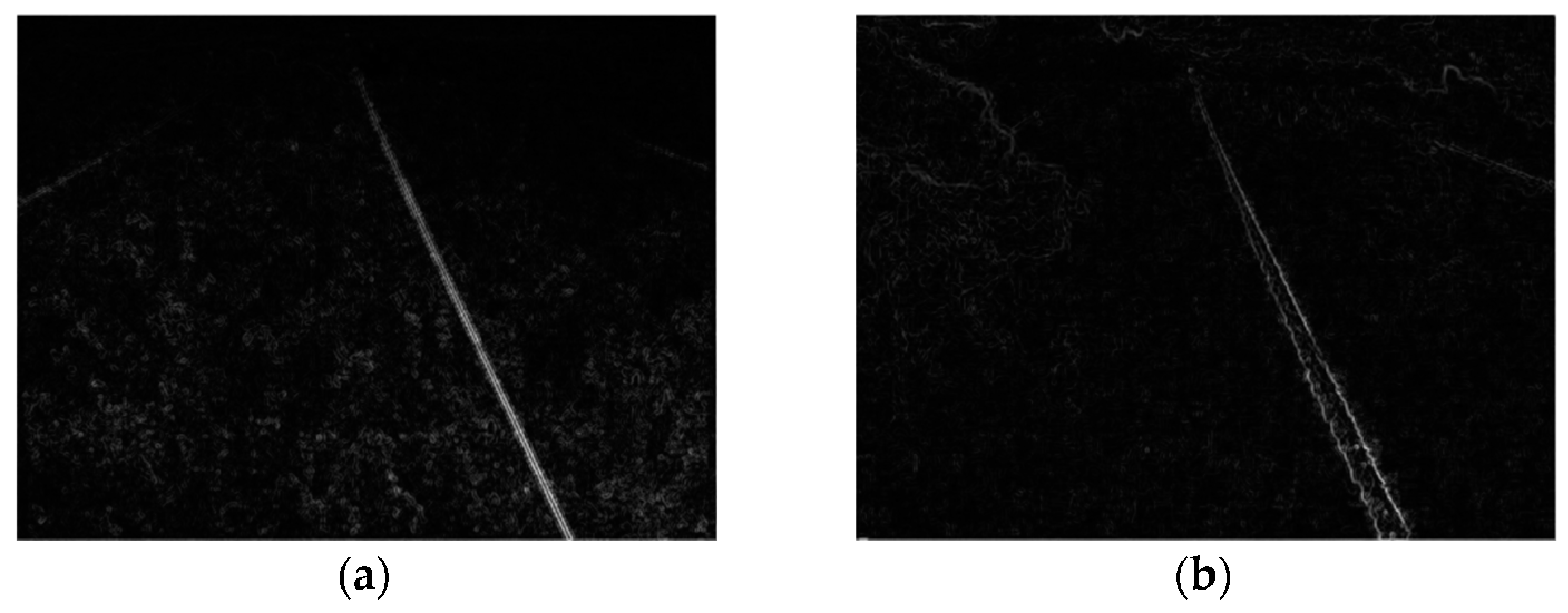
Figure 6.
The four sectors of the circumference.

Figure 7.
The grayscale images after non-maximum suppression. (a) The grayscale image of an un-iced power transmission line after non-maximum suppression; (b) The grayscale image of an iced power transmission line after non-maximum suppression.
Figure 7.
The grayscale images after non-maximum suppression. (a) The grayscale image of an un-iced power transmission line after non-maximum suppression; (b) The grayscale image of an iced power transmission line after non-maximum suppression.

Figure 8.
The three-dimensional display image of the gradient amplitude, among them, the pixel coordinates of the image are used as the x-axis and y-axis, and the gradient amplitude (or gray value) of the pixel is used as the z-axis. (a) The gradient amplitudes of pixels in Figure 7a; (b) The gradient amplitudes of pixels in Figure 7b.

Figure 9.
The binary image edges after dual threshold edge detection. (a) The binary image edges of an un-iced power transmission line; (b) The binary image edges of an iced power transmission line.
Figure 9.
The binary image edges after dual threshold edge detection. (a) The binary image edges of an un-iced power transmission line; (b) The binary image edges of an iced power transmission line.

Figure 10.
Correspondence between image (a) space i-j and (b) parameter space k-b.
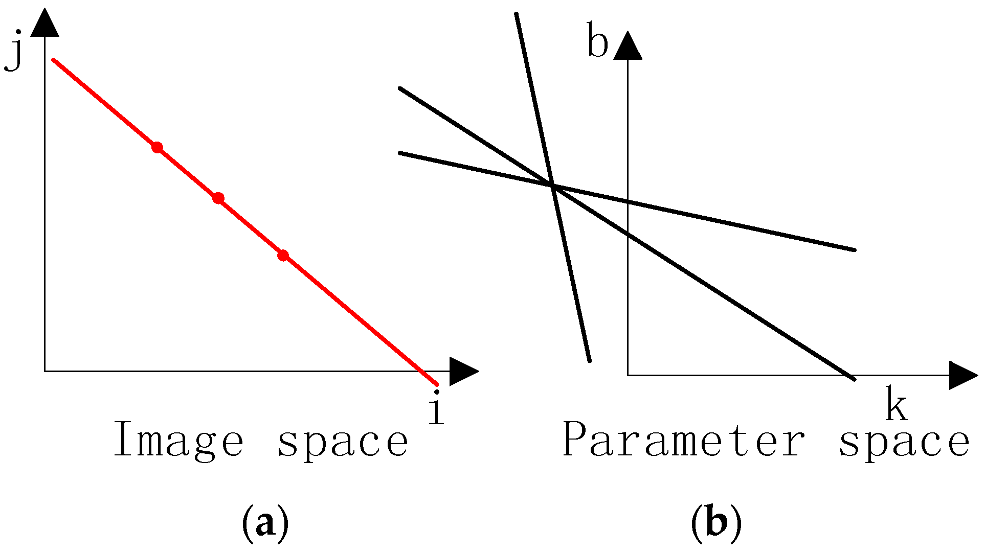
Figure 11.
The correspondence between the image (a) space i-j and (b) the parameter space -.

Figure 12.
Accumulated statistical results after Hough transform. (a) The accumulated results of Figure 9a after Hough transform; (b) The accumulated results of Figure 9b after Hough transform.
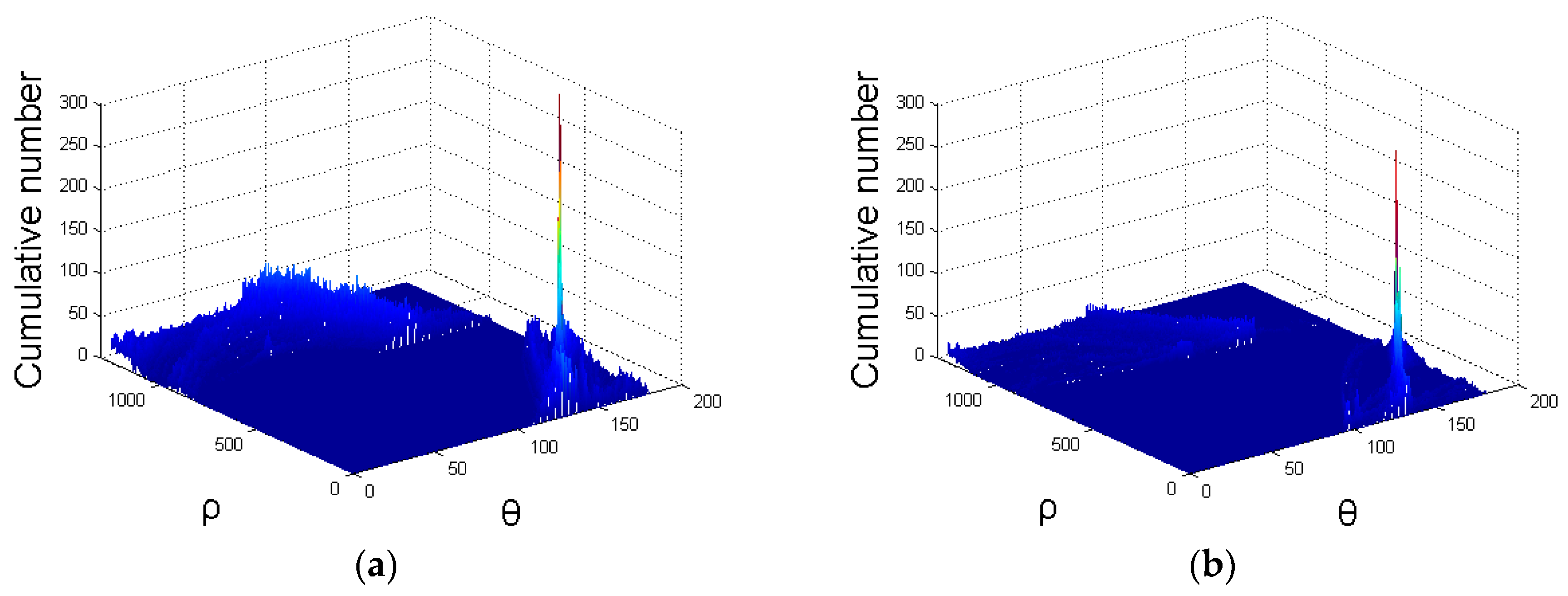
Figure 13.
The rough positioning results of the power transmission line edges after Hough transform. (a) The rough positioning results of an un-iced power transmission line edges; (b) The rough positioning results of an iced power transmission line edges.
Figure 13.
The rough positioning results of the power transmission line edges after Hough transform. (a) The rough positioning results of an un-iced power transmission line edges; (b) The rough positioning results of an iced power transmission line edges.

Figure 14.
Accurate positioning results of the power transmission line edge (a) The accurate un-iced power transmission line edges; (b) The accurate iced power transmission line edges.
Figure 14.
Accurate positioning results of the power transmission line edge (a) The accurate un-iced power transmission line edges; (b) The accurate iced power transmission line edges.
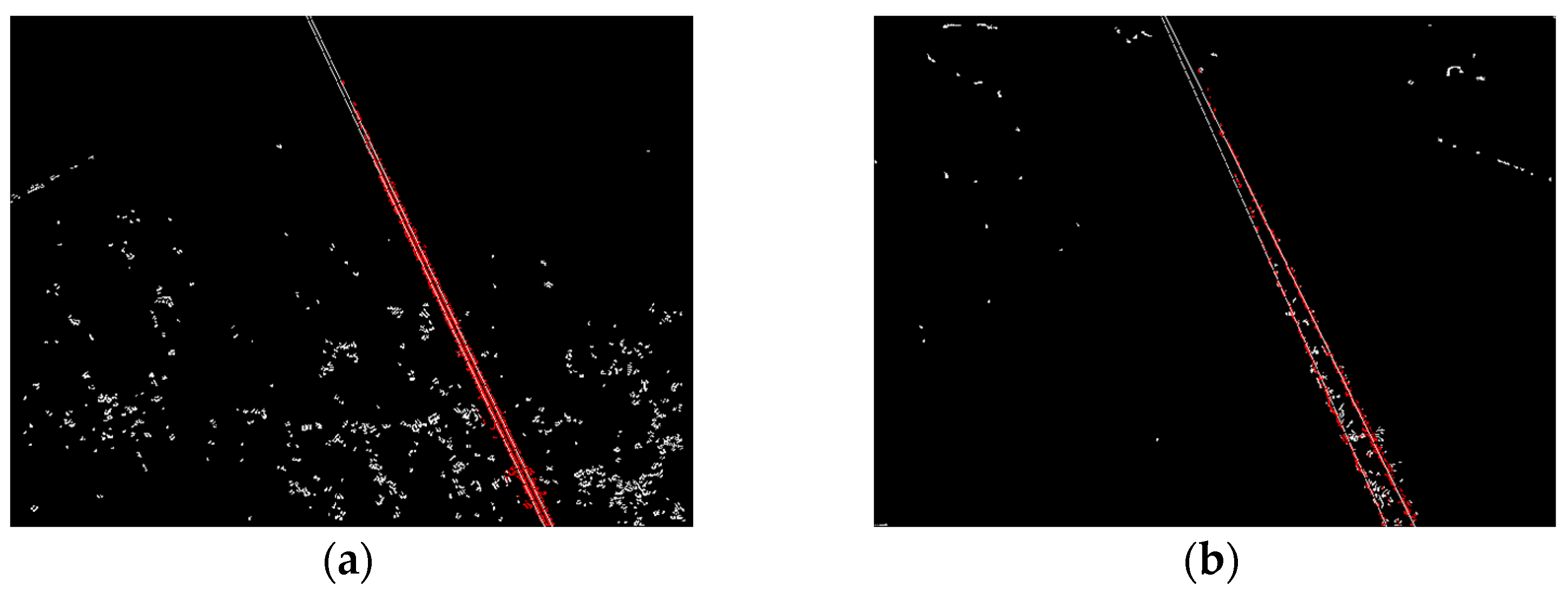
Figure 15.
Accurate positioning results are placed into the original color images. (a) Accurate positioning result of an un-iced power transmission line; (b) Accurate positioning result of an iced power transmission line.
Figure 15.
Accurate positioning results are placed into the original color images. (a) Accurate positioning result of an un-iced power transmission line; (b) Accurate positioning result of an iced power transmission line.

Figure 16.
Imaging principle of the camera.

Figure 17.
Schematic diagram of the power transmission lines. (a) Image schematic diagram of an iced power transmission line; (b) Image schematic diagram of an un-iced power transmission line.
Figure 17.
Schematic diagram of the power transmission lines. (a) Image schematic diagram of an iced power transmission line; (b) Image schematic diagram of an un-iced power transmission line.

Table 1.
Resetting gradient angles.
| Sector | Gradient Angle/Degree | Gradient Angle After Reset/Degree |
|---|---|---|
| 0 | (0, 22.5) and (157.5, 180) | 0 |
| 1 | (22.5, 67.5) | 45 |
| 2 | (67.5, 112.5) | 90 |
| 3 | (112.5, 157.5) | 135 |
Table 2.
Power transmission line edge detection results.
| Detection Results | A’C’/Pixel | AC/Pixel |
|---|---|---|
| Least squares Hough transform | 8.46 | 27.21 |
| Manual count | 8 | 28 |
Table 3.
Calculated icing thickness based on different image recognition methods.
| Image Recognition Method | Real Icing Thickness/mm | A/mm | B/mm | C/mm | D/mm |
|---|---|---|---|---|---|
| Icing thickness | 21.22 | 30.62 | 29.14 | 41.71 | 17.97–57.47 |
Notes: Method A is the least squares Hough transform method. When image edges are obtained, method B simply averages the vertical coordinates of the upper outline pixels and lower outline pixels of power transmission line as power transmission line edges distance [10,24]; Method C searches for the distance between the upper and lower power transmission line edge pixels to obtain the maximum distance as the power transmission line edges distance [25], and then method D uses the Hough transform to fit two random points on the power transmission line edges to calculate the slope of the power transmission line edges [16].
© 2017 by the authors. Licensee MDPI, Basel, Switzerland. This article is an open access article distributed under the terms and conditions of the Creative Commons Attribution (CC BY) license (http://creativecommons.org/licenses/by/4.0/).
Share and Cite
MDPI and ACS Style
Wang, J.; Wang, J.; Shao, J.; Li, J. Image Recognition of Icing Thickness on Power Transmission Lines Based on a Least Squares Hough Transform. Energies 2017, 10, 415. https://doi.org/10.3390/en10040415
AMA Style
Wang J, Wang J, Shao J, Li J. Image Recognition of Icing Thickness on Power Transmission Lines Based on a Least Squares Hough Transform. Energies. 2017; 10(4):415. https://doi.org/10.3390/en10040415
Chicago/Turabian StyleWang, Jingjing, Junhua Wang, Jianwei Shao, and Jiangui Li. 2017. "Image Recognition of Icing Thickness on Power Transmission Lines Based on a Least Squares Hough Transform" Energies 10, no. 4: 415. https://doi.org/10.3390/en10040415
Note that from the first issue of 2016, this journal uses article numbers instead of page numbers. See further details here.