Pareto-Efficient Capacity Planning for Residential Photovoltaic Generation and Energy Storage with Demand-Side Load Management


Department of Electronics and Communication Engineering, Hanyang University, Ansan 15588, Korea
*
Author to whom correspondence should be addressed.
Energies 2017, 10(4), 426; https://doi.org/10.3390/en10040426
Submission received: 6 February 2017
/
Revised: 13 March 2017
/
Accepted: 17 March 2017
/
Published: 23 March 2017
Abstract
:Optimal sizing of residential photovoltaic (PV) generation and energy storage (ES) systems is a timely issue since government polices aggressively promote installing renewable energy sources in many countries, and small-sized PV and ES systems have been recently developed for easy use in residential areas. We in this paper investigate the problem of finding the optimal capacities of PV and ES systems in the context of home load management in smart grids. Unlike existing studies on optimal sizing of PV and ES that have been treated as a part of designing hybrid energy systems or polygeneration systems that are stand-alone or connected to the grid with a fixed energy price, our model explicitly considers the varying electricity price that is a result of individual load management of the customers in the market. The problem we have is formulated by a D-day capacity planning problem, the goal of which is to minimize the overall expense paid by each customer for the planning period. The overall expense is the sum of expenses to buy electricity and to install PV and ES during D days. Since each customer wants to minimize his/her own monetary expense, their objectives look conflicting, and we first regard the problem as a multi-objective optimization problem. Additionally, we secondly formulate the problem as a D-day noncooperative game between customers, which can be solved in a distributed manner and, thus, is better fit to the pricing practice in smart grids. In order to have a converging result of the best-response game, we use the so-called proximal point algorithm. With numerical investigation, we find Pareto-efficient trajectories of the problem, and the converged game-theoretic solution is shown to be mostly worse than the Pareto-efficient solutions.
1. Introduction
Customers are being provided high-quality and economically-efficient electricity supply by smart grids. Smart grids are electricity networks that use digital and other advanced technologies to monitor and manage the transport of electricity from all generation sources to meet the varying electricity demands of end-users [1]. Moreover, future smart grids are expected to contribute to ensuring the efficient and sustainable use of natural resources and then reducing carbon emissions [2].
Attached to smart grids connecting an electricity service provider, a smart meter at the customer side schedules the activation of home appliances and controls, if any, residential energy generation and storage systems, which is so-called demand-side load management [3]. The residential version of demand-side load management typically aims at reducing and/or shifting energy consumption [4]. Furthermore, increasing forces and policies that promote green-energy technologies, such as wind, solar-photovoltaic (PV) generation and energy storage (ES), to be installed at home, cause residential load management to be more complicated [5].
Many load management methods without considering energy generation and storage have been proposed (e.g., [6] and the references therein). A main theme of these methods is how to encourage distributed customers to individually and voluntarily manage their load, for example to reduce their consumption at peak hours. Real-time pricing is a possible option that lets the price of electricity vary at different hours of the day and facilitates interactions between the service provider and customers. The price released by the service provider is assumed to be immediately responsive to the load scheduling from customers, and then, customers re-establish their consumption schedule according to the price. With such interactions, the load management could be performed in a distributed way [7,8]. In [6], the interaction is not only by pricing, but by a specially-designed incentive method, while keeping the customers’ overall expense from increasing.
In [9], a residential load management method for customers owning distributed energy generation and ES devices is proposed in the form of day-ahead optimization. The main objective of these customers is to reduce their monetary expense during the time period of analysis by producing and/or storing energy rather than just purchasing their energy needs from the grid. The problem is formulated as a noncooperative Nash game, and equilibrium points are identified with convex cost functions. When considering time-shiftable appliances, the load management problem becomes a mixed integer programming problem and usually is hard to solve [6,10], and the convergence to a Nash equilibrium is not easily guaranteed. Especially focusing on non-interruptible and non-power-shiftable devices that are time-shiftable, an efficient solution method that solves a mixed integer programming problem with distributed renewable energy generation and ES devices is provided in [11].
In the existing works on residential load management mentioned above, the capacity of energy generation and storage is assumed to be given and fixed. To provide an optimal design on the capacity, techno-economic methods are developed in [12,13,14]. Since the electricity supplied only by new and renewable energy systems is not stable or economically not feasible, dispatchable fuel energy systems are added as supplementary electricity sources. For these hybrid energy systems, many works have dealt with an optimal allocation problem of the sizes between PV, ES, wind generation, diesel/gas turbines, bio-diesel generators and/or combined heat and power systems [15,16,17,18,19]. Extending these results, the configuration problems for polygeneration or multi-generation also have been investigated by many authors. Polygeneration represents a further integrated hybrid energy system that simultaneously provides diverse products, such as heating, cooling, as well as electricity [20]. Moreover, fresh water obtained from a local desalination unit could be a product of a polygeneration system. Definitely, renewable energy sources play a critical role in designing a polygeneration system. The works in [20,21,22,23] have provided an optimal configuration of various levels and combinations of polygeneration.
Though optimal sizing of PV and ES has been treated as a part of designing hybrid energy systems and polygeneration systems, it has been rarely considered in the context of residential load management in smart grids. The economic efficiency of installing PV and ES at home should be dependent on the varying electricity price that is a result of individual load management of the customers in the market. Thus, if a house or a building can access the electricity grid and does not have a strict mission of establishing a 100% self-produced energy system, the market price of electricity should be considered in determining an adequate (perhaps economic) size of residential renewable energy systems. In other words, the load-management behavior of other customers is an important factor when determining an optimal size of PV and ES at my home, respectively.
Motivated by the above finding, we in this paper investigate an optimal size of PV and ES, respectively, as a part of smart grids where the unit installation and maintenance cost of PV and ES, respectively, is given and the electricity price is dynamically determined as a result of the load request from all customers. Considering aggressive government polices that promote installing renewable energy sources in many countries [24,25,26] and the recent development of small-sized PV and ES systems for easy use in residential areas [1,27], we understand that the optimal sizing of residential PV and ES is a timely issue.
The problem we have is formulated by a D-day capacity planning problem, the goal of which is to minimize the overall expense paid by each customer for the planning period. The overall expense is the sum of expenses to buy electricity and to install PV and ES during D days. Based on a day-ahead optimization practice of residential load management, per-hour electricity price is interactively determined by a quadratic cost function of producing the aggregate per-hour load request from all customers. On the other hand, the prices of installing PV and ES are assumed given and fixed. The overall expense is evaluated in the form of the present value at the starting time of the planning period. Since each customer wants to minimize his/her monetary expense, their objectives look conflicting, and we first regard the problem as a multi-objective optimization problem. With numerical investigation, we find Pareto-efficient trajectories of the problem. As we already discussed, game-theoretic approaches are widely used in looking for a solution of residential load management. We secondly formulate the problem as a D-day noncooperative game between customers, which can solve the multi-objective problem in a distributed manner and thus is better fit to the pricing practice in smart grids. In order to have a converging result of the best-response game, we add a regularizing cost term to the individual expense, like in [28], which forms the so-called proximal point algorithm [29]. With numerical investigation, the converged game-theoretic solution is shown to be worse than (or dominated by) the Pareto-efficient solutions. This means that a customer can reduce his/her expense, from the equilibrium, without increasing the expense of the other customers. In the simulation, it is seen as optimal if 54.52% of the load is covered by PV and ES systems, for which the expense caused by purchasing the equipment is about 57.48% of the total daily expense of the home considered. Moreover, when a customer optimally decides to install PV and ES systems, the expense of the other customers is also decreasing by 39.67% since the installation allows the electricity price be reduced.
The rest of this paper is organized as follows. Section 2 introduces our system model that consists of an overall smart grid network, a PV generation system, an ES system and residential load control. In Section 3, the capacity planning problem is formulated in the forms of multi-objective optimization and a noncooperative game, respectively, and how to obtain Pareto-efficient solutions and converging game-theoretic solutions is also discussed. Section 4 provides some results from the numerical investigation, which includes the optimal sizes of PV and ES according to the purchasing cost of the equipment, respectively, a comparison of load demand and electricity price between with and without the installation of PV and ES and a comparison between Pareto-efficient and game-theoretic solutions. In the end, Section 5 concludes this paper. The main notations used in this paper are listed in Table 1.
2. System Model
2.1. Smart Grid Model
We consider a smart power system that consists of an energy service provider and multiple residential customers. As shown in Figure 1, the smart power system has been equipped with a two-way communication link that enables the service provider and the customers to exchange information with each other. Each customer can install his/her own photovoltaic generation and energy storage system (PVS and ESS, respectively) at home. Additionally, we assume that each customer is equipped with a smart meter that has a home load management (HLM) capability for scheduling the household energy consumption, as well as PVS and ESS if they exist. The smart meter is connected to the power lines coming from the service provider and coming from home-located PVS and ESS, respectively.
Let us define to be a set of customers in the power system. We assume that is divided into three disjoint subsets: , and , where denotes a set of customers that are willing to install PVS and ESS at their home, denotes a set of customers that are already equipped with PVS and ESS and denotes a set of customers that currently do not consider PVS and ESS. For each customer , the HLM module in the smart meter computes the per-slot energy load profile , defined as the energy that needs to be purchased by customer n to supply his/her appliances at time slot h. Without loss of generality, we assume that the time granularity is one hour, i.e., , where for one-day scheduling. We also assume that each HLM module does a day-ahead scheduling of residential energy consumption at the beginning of Time Slot 1. When we consider long-term multiple-day scheduling for capacity planning, superscript denotes a specific day. That is, denotes the energy load of customer n at h hour of d day. However, superscript is usually ignored for brevity, unless it is confusing.
After HLM obtains , the smart meter sends the daily load profile to the service provider. Let be an aggregate load through the power system at time h. The cost of generating and distributing the required electricity demand from the customers is evaluated by the service provider. We assume a quadratic cost function widely accepted in the smart grid literature [9,28]:
where (>0) is a constant cost coefficient. We assume that could vary time by time according to the global (national) electricity-plant operation schedule, as well as the availability of intermittent energy sources. It is noted that the cost function we consider in this paper can be either an actual energy cost for producing the required load or just an artificial cost that is used by the service provider to obtain adequate control on the electricity load [28].
To complete the day-ahead scheduling, the service provider announces daily price profile through the communication network connecting all of the customers, based on an average cost obtained from (1), such that:
With , HLM modules re-optimize their energy consumption schedule and send the resulting load profile back to the service provider. Then, the price profile changes, and the optimization process in the HLM module is iteratively re-evoked. Since the cost function we assume in this paper is convex, such an iterative procedure could finally converge to a Nash equilibrium when the problem dealt with by the HLM module is also convex [28]. It is worth noting that the problem we investigate in this paper is not a day-ahead load management, but a long-term capacity planning, as an example, a 10,000-day planning for which a day-ahead optimization with the dynamic daily price profile serves as a subroutine.
2.2. Photovoltaic Generation Model
Let (≥0) be the per-slot photovoltaic energy generation profile. We assume that is upper-bounded by the area (i.e., the array surface area) of solar panels installed by customer n, such that:
where (>0) is an exogenous parameter that represents an hourly power production efficiency of PVS. is forecasted and given to the system, which mainly depends on the availability of the solar radiation that is a function of the sky clearness index [30,31].
2.3. Energy Storage Model
Let (≥0) be per-slot energy storage profile measured at the end of time slot h, which is a stock variable. Let two flow variables (≥0) be per-slot energy charging and discharging profile, respectively. Then:
where is a leakage rate that represents the decrease in the energy level with the passage of time. If new charging during time slot h, the charged level of ESS reduces to from at the end of time slot h. To complete the equation in (4), we should define an auxiliary variable since . represents an initial state of ESS. For a day-ahead optimization, with an arbitrary small positive constant , a constraint: is imposed to ensure that ESS keeps the desired level of charge at the end of the time horizon of analysis [9] and to prevent any type of free leakage from or free influx into ESS. We in this paper adopt a strict constraint, such that:
However, since customer in our problem has installed a new ESS at the beginning,
When customer n considers installing or has already installed ESS with capacity :
Furthermore, certain inefficiency could arise when charging and discharging energy into and from ESS, respectively. Let be the amount of electricity load to be used to charge ESS. is not wholly charged, but only a part of it is charged. To capture this effect, we introduce a parameter representing charging efficiency. Then, . On the other hand, discharged amount cannot be used by the appliances as a whole, but only a part of it is used, where is called the discharging efficiency.
2.4. Residential Load Control by HLM Module
For each customer , let denote a set of household appliances, such as heaters, dish washers, electric vehicles, etc. For appliance , let us denote by = an energy consumption scheduling vector of the appliance, where (≥0) is the scheduling variable at hour h. The total load needed by the n-th customer is then constrained by:
where is the energy generated in PVS at hour h and immediately used at that time slot, and hence, . Furthermore, denotes the electricity requirement due to charging ESS for future use, and obviously .
For each appliance , it has the daily requirement that should be met by its total daily energy consumption:
Let us assume that the appliances can be described by three types of energy consumption patterns: non-shiftable, power-shiftable and time-shiftable. For non-shiftable appliances, such as heaters, the appliances have fixed energy requirement during a fixed operation period from to . Let denote the set of activation hours. The consumption requirement by non-shiftable appliances can be written as:
For power-shiftable appliances such as electric vehicles, the smart meter will schedule flexible power between a standby power, , and a maximum working power, . Thus, the scheduling is constrained by:
The scheduling period could be either time-shiftable or non-time-shiftable. For a non-time-shiftable case, Constraint (11) should be satisfied for with a given working period .
For a time-shiftable case, the smart meter is able to control the switch of electricity supply corresponding to the energy consumption pattern during the scheduled period. If appliance has a fixed energy consumption pattern , the schedule result has to be exactly the same as one of the cyclic shifts, where subscript h denotes the starting time of the shift of that pattern. All of the possible shifts for the vector and, hence, all the possible can be put in a matrix form as:
Let us define a binary integer vector as the switch control for the time-shiftable appliance. Time-shiftable appliances are assumed not to be allowed to stop once they start, and the constraint can be written as:
Additionally, the schedule plan can be written as:
in (12) is also used in [10] to describe time-shiftable, but non-power-shiftable scheduling. If a time-shiftable appliance is power-shiftable at the same time as electric vehicles, let us denote by and the lower and the upper bound matrix of energy consumption, respectively. Each element of and is filled with and not by the fixed consumption plan, respectively. Then, the schedule should be constrained by:
where ≤ should hold for the component-wise operation of the vectors.
3. Capacity Planning Problem
3.1. Multi-Objective Formulation
We are mainly focusing on customers in who consider installing PVS and ESS in the future. Let and be a present unit cost of installing and at home of customer , respectively. We assume that installed PVS and ESS have a life time of D days, respectively, and hence, the period of our planning problem is also D days. The unit cost includes the equipment cost, as well as the maintenance cost during D days. We also assume that the payment of every customer for the purchased load is made at the end of each day. Then, the payment for a specific day d is:
Thus, for customer , the total cost paid over D days in the present value is:
where r is the market rate of interest per day and denotes the full set of load required by customer j during D days. For customer , the total present cost is:
It is noted that customer k in already paid for the previously installed equipment of PVS and ESS, and we ignore this cost in (19), since it is constant after and are determined; and thus, it does not affect the cost minimization process afterwards. Furthermore, we assume that the life time of PVS and ESS already installed at customer is not shorter than D days.
For customer , let us denote by a set of feasible load scheduling with nonnegative PVS and ESS capacities, which is summarized in Table 2. For customer , the feasible region is similarly determined as , except that and are given as a constant, respectively, and denoted by . If , the customer does not have constraints regarding PVS and ESS, and the feasible load scheduling is denoted by . For notational brevity, let us further denote the decision vector for customer n by:
where and represent the already determined capacity of PVS and ESS for , respectively. It is noted that , especially for customer .
When the electricity demand for home appliances and production efficiency of PVS and ESS are given for D days, the problem we have is:
(MP) is a multi-objective programming problem with n conflicting attributes. Each customer tries to minimize his/her present-valued cost, but the respective costs are tightly coupled mainly due to the cost function defined in (1). It is worth noting that the constraints set in (22) are decoupled according to the customer.
3.2. Pareto-Optimal Solution
A usual way to define an optimal solution of problem (MP) is Pareto-optimality. Let be an aggregate feasible solution of (MP). Then, is said to be Pareto-optimal (or a noninferior solution) if there exists no other feasible solution such that for with strict inequality for at least one n [32,33]. There are certain common approaches for characterizing Pareto-optimal solutions. We adopt a weighted scalarization of (MP) in this paper. Let , where , be a vector of nonnegative weights such that . Then, a weighted problem is:
Since the long-term cost function is quadratic and strictly convex, (WMP)is a mixed integer quadratic convex optimization problem and can be solved by many solution tools, such as GAMS. Let be a solution of problem (WMP) for given (≥0). Then, is a Pareto-optimal solution if either one of the following two conditions holds: for all n; or is a unique solution [33].
3.3. Game-Theoretic Approach
A day-head load scheduling in HLM is usually formulated by a game among customers. Our problem also can be seen as a long-term game. The D-day scheduling of a customer depends on how he/she and all other customers schedule the electricity consumption, generation and charge during the days. Let us denote by the aggregate feasible solution containing the load, generation and charge schedules of all of the customers except customer n. Then, the problem can be formulated as an N-player noncooperative game. Each customer selects his’her own strategy in the feasible set of load schedules. The goal of each customer as a player in the game is to minimize his/her payoff function given the aggregate load scheduling and capacity planning of the other customers as . Let us denote by such a payoff function. Then, customer n tries to solve:
Unlike the problems (MP) and (WMP), problem (GP)is distributed in a sense that, with the information from the other customers or a certain central unit, each customer can get his/her own optimal strategy in a distributed way. In practice, the information needed is only the total load per hour for the planning period in order to construct the cost function. When he/she has , serves as a fixed coefficient of the objective function during the distributed payoff optimization.
Regarding the formulated games, two questions are usually raised: (i) does there exist a solution that is a so-called Nash equilibrium that is a feasible aggregate solution from which no single customer has unilateral incentive to deviate [6]; and (ii) does the iterative and distributed search of by (GP) converge to a Nash equilibrium, starting from an arbitrary load schedule? We leave rigorous answers to our problem for future study, but are going to numerically investigate the convergence property in this paper.
Some related results on day-ahead optimization as noncooperative load scheduling games can be summarized as follows. If there is no time-shiftable appliance at home, no energy generation and no storage and if the cost function is quadratic, then a Nash equilibrium is unique and optimal, and furthermore, a distributed algorithm converges to the equilibrium [28]. With energy generation and storage, when the hourly load required for home appliances is scheduled and fixed, the game-theoretic formulation of optimizing the level of energy generation and charge has multiple Nash equilibria, though they have the same values in the payoff functions [9]. When time-shiftable appliances are considered, a day-ahead scheduling at the HLM module becomes a mixed-integer programming problem [7], and it is not clear that the selfish game strategy of customers may produce a good solution that is Pareto-optimal [11]. Without the facilities of energy generation and storage, [8] provides a sketch of the optimality and convergence of a game-theoretic schedule including time-shiftable appliances.
In order to regularize the convergence if it takes too long or is not possible, we use a proximity point algorithm for (GP), which is described in Table 3. In Table 3, is the so-called proximity control parameter that could be set with a fixed constant or be adjusted according to the solution strategy [34]. In this method, is updated and used as a part of the regularized payoff function. When the algorithm terminates, the most recent is regarded as a solution.
4. Numerical Results
4.1. Simulation Setup
A set of planning simulations has been carried out using the CPLEX solver with GAMS. We assume that the period of planning is a typical consecutive three days, 72 h, for illustrative purpose. In the simulation, we consider three types of HLM denoted by HLM1, HLM2 and HLM3, which are customers in the sets of and , respectively. The electricity requirement for appliances installed in each home is depicted in Table 4. Appliances are divided into three classes depending on the characteristics on energy demand: non-time-power shiftable (NTS), power shiftable (PS) and time shiftable (TS). We have designated that the amount of daily electricity requirement is different according to the customers. HLM1 requires the largest, HLM2 the second and then HLM3. To let each of the three days represent a specific day in a year, we assume that heaters are operating only for Day 1 (i.e., winter), air conditioners only for Day 3 (i.e., summer) and none of them for Day 2 (i.e., spring or fall). The other appliances should work every day.
As the coefficient of quadratic cost function, we use and = 9.66 as in [23]. Since HLM1 and HLM2 are in sets of and , respectively, they are equipped or will be equipped with PVS and their hourly production efficiency in PVS, which is given in Figure 2. We also assume that the already installed capacities of PVS and ESS for HLM2 are 4 kW and = 3 kWh (According to Equation (3), in this paper indicates storage capacity. Inverter capacity is not precisely considered for brevity in this paper. However, the per-slot energy charging and discharging profile, and , should be less than or equal to by (4). And thus and by nonnegativity of , which means that we implicitly assume the inverter capacity also to be and, hence, 3 kW for HLM2 in the simulation.) For ESS parameters, we assume that , . For objective functions, we assume % and cents/kW, unless clearly stated.
4.2. Pareto-Efficient Planning
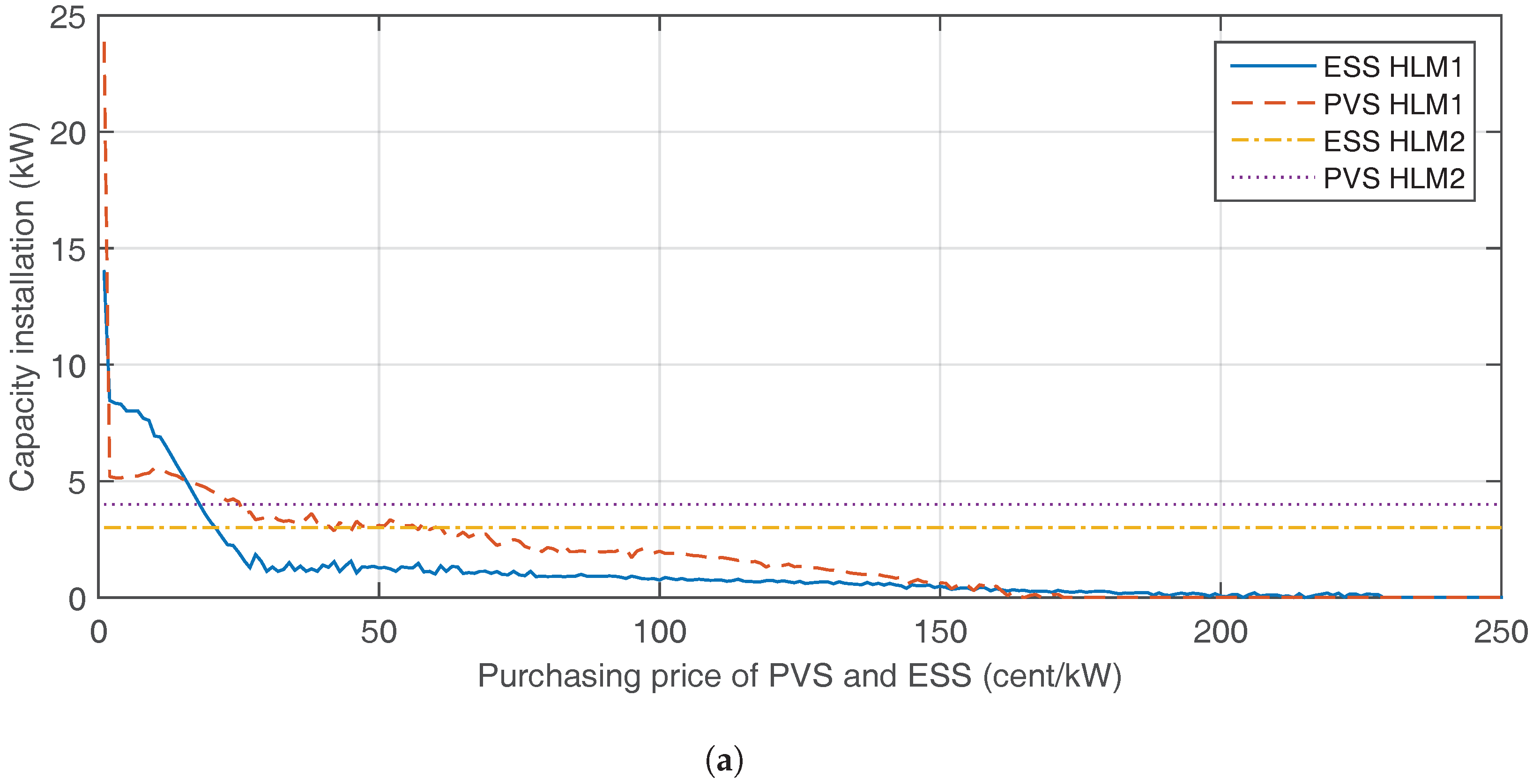
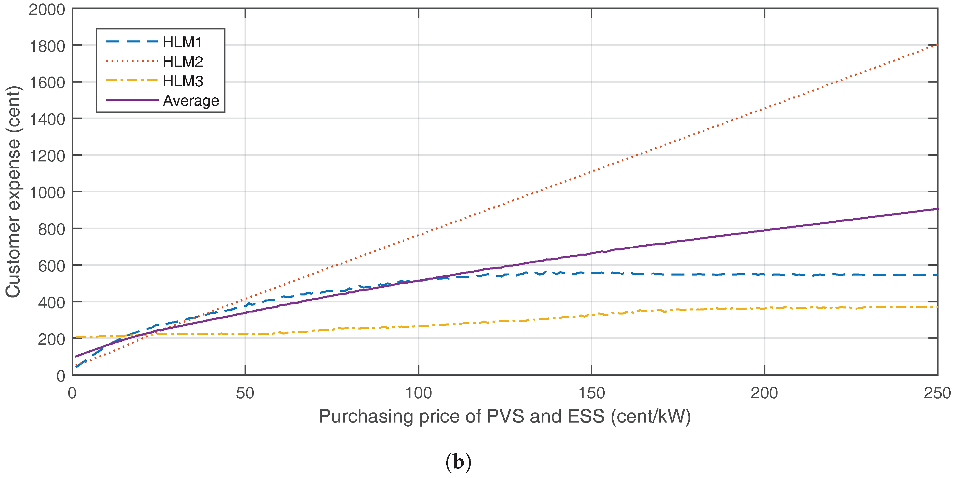
It is noted that HLM1 considers new PVS and ESS to install at home in our simulation. The capacities to be installed are obviously a function of the related prices: electricity prices, market rate of interest (r), purchasing prices of PVS and ESS (). The electricity prices are determined by interactions between customers and the service provider, as described in Section 2.1. When we set %, Figure 3a shows optimal capacities of PVS and ESS, respectively, that could be installed at HLM1 according to the purchasing prices. We assume for any customer n. The objective function used to resolve conflicting desires of the customers in the market is the sum of expenses by the customers. The straight lines in the figure show the capacities already installed at HLM2: 4 kW and 3 kW of PVS and ESS, respectively. It is seen that the optimal capacities decrease when the purchasing price increases. At cents, ESS is not installed any more; neither is PVS at cents. It is noted that the small fluctuations in capacities seen when the price increases are due to multiple solutions of the mixed integer problem we have. As seen in Figure 3b, the average expense, however, monotonically increases as the purchasing price increases. In Figure 3b, the total and individual expenses are shown according to the purchasing price, respectively. Though HLM2 is assumed to already install PVS and ESS, the cost of equipment is added to the total expense for comparison in the figure. Every expense increases as the price increases. Especially, the expense by HLM3 that does not consider PVS and ESS also increases as the equipment price increases. This is because the lesser capacity installation in HLM1 due to the higher cost makes the electricity requirement from the grid increase and the electricity price higher. By 3.28-kW and 1.20-kW installation of PVS and ESS by HLM1 at the purchasing price of 224.42 cents, HLM3 reduces his/her expense by 27.98% compared with the expense without PVS and ESS at HLM1. This means that the economically-efficient decision of HLM1 contributes to reducing the expense for HLM3 and, thus, increasing social welfare. It is worth noting that, if the maximum power is 275 W with a PVS panel of height 2 m and width 1 m, as in [23], to install 3.28 kW PVS at home, we need 12 PVS panels and, thus, 24 square meters.
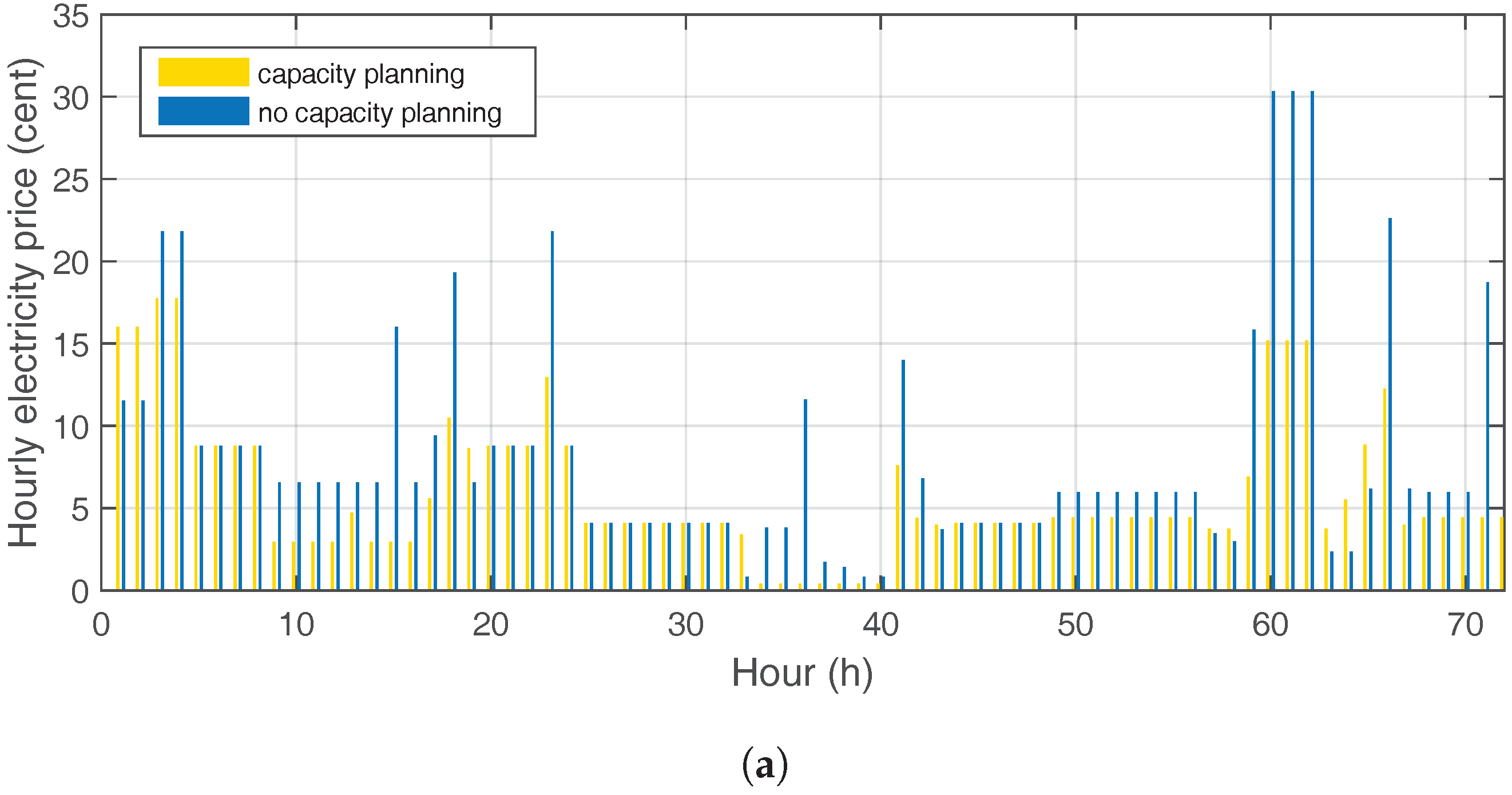
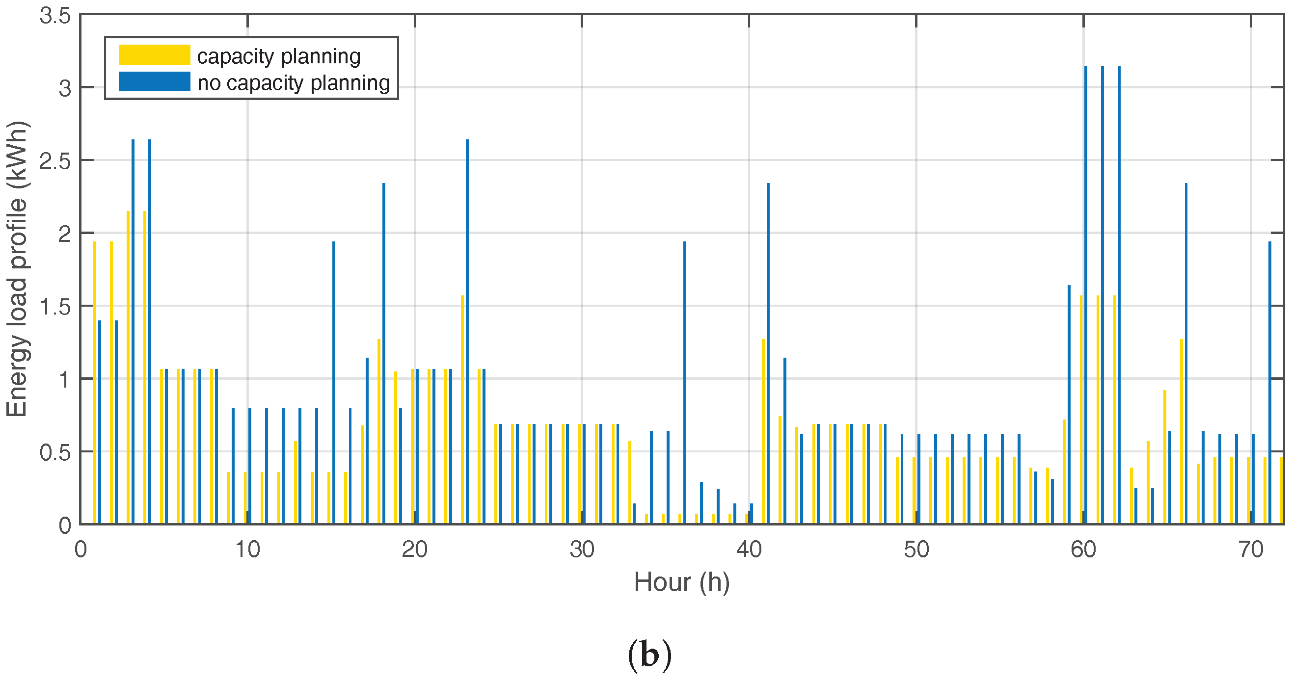
Figure 4a,b compares the electricity price and the load per hour with and without PVS and ESS in HLM1, respectively. With the purchasing price of cents/kW, the optimal sizes of PVS and ESS are 3.28 and 1.20, respectively. “No capacity planning” refers to a result of HLM1’s decision not to install PVS and ESS. The price and load per hour with the capacity planning is mostly lower than or equal to that from no capacity planning. Especially, at the initial stage of planning period (Hours 1–4), electricity consumption is high since ESSs in HLM1 and HLM2 store the energy in order to use it for Hours 3 and 4 when the demand is at a peak due to the non-time shiftable requirement of boilers. With PVS and ESS, the peak load is reduced from 3.14 down to 2.15 and so is the price from 30.33 down to 17.75.
Figure 5a shows the the average amount of electricity generated by PVS and immediately used by appliances at HLM1, and Figure 5b shows the level of stored energy in ESS and the charging and discharging flows in each hour at HLM1. In Figure 5a, different patterns are seen in the daily usage of electricity generated by PVS, which is due to multiple-day planning. If a day-ahead optimization is considered, the energy consumption pattern is identical day by day, unless the amount of solar generation changes. In HLM1, PVS generates 61.66% of the total energy consumed during the period of planning, among which 42.93% is immediately used and 18.73% is stored and used later. When ESS is charged, the source of electricity is either PVS or the grid. In comparing Figure 5a,b, 28.79% of electricity that is stored in ESS is from the grid, which means that ESS is working not just to store the energy from PVS, but to smooth the electricity load in the period of planning by purchasing the energy adaptively.
4.3. Game-Theoretic Planning
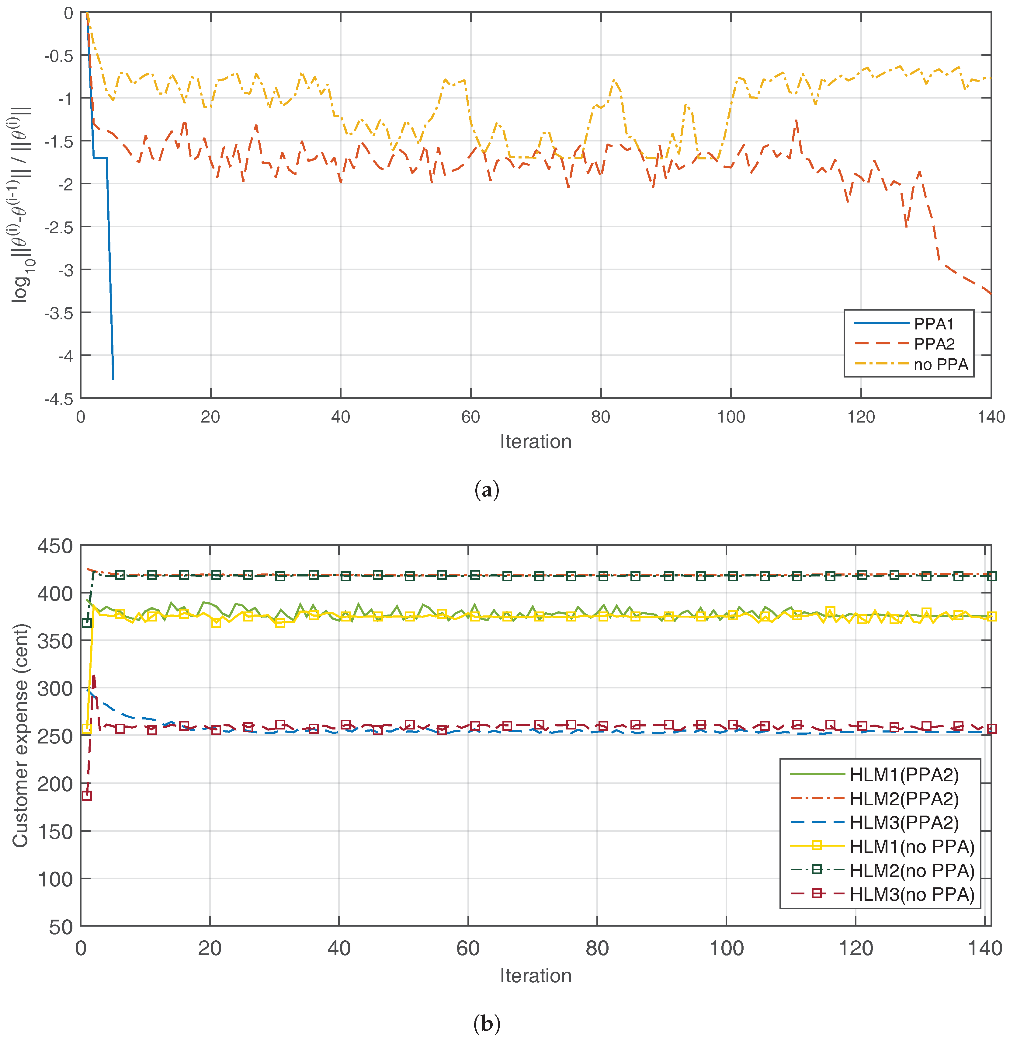
In this subsection, a noncooperative game with the customers of the exact same configuration in Section 4.2 is investigated. Figure 6a illustrates the convergence behavior of the two solution approaches: one is with the proximal point algorithm (PPA) provided in Table 3, and the other is without it (referred to as “no PPA”). In implementing the proximal point algorithm, we test two rules of updating the proximity control parameters: an adaptive method by updating (referred to as PPA1) and a fixed method by setting as a constant (referred to as PPA2), provided as in [11]. We use as a convergence criterion. Figure 6a PPA1 converges very quickly at Iteration 6, and PPA2 finally converges at Iteration 140. However, “no PPA” seems to be hard to converge. Figure 6b shows the behavior of the expenses by PPA2 and “no PPA” for each customer corresponding to Figure 6a, which are optimized in a distributed way. The expenses achieved by PPA1 are 375.43, 417.60 and 260.58 for HLM1, HLM2 and HLM3, respectively, which are not depicted in the figure, since PPA1 converges very quickly. As seen in the figure, the expenses are almost unchanged after Iteration 100 in PPA2 and are 375.45, 419.28 and 253.61 for HLM1, HLM2 and HLM3, respectively. For “no PPA”, the expenses of HLM1 and HLM3 fluctuate over iterations. “No PPA” generates 375.29, 417.46 and 256.47 for HLM1, HLM2 and HLM3 at Iteration 140, respectively, which is obviously dominated by the solution obtained by PPA1. By comparing Figure 6a,b, we can see that PPA1 and PPA2 converge to solutions, though they are different, providing a very close result in the sense the expenses are nearly similar and one solution is not dominated by the other.
Figure 7 shows the average load per hour from the game-theoretic solution of PPA1. In this figure, it is seen that the first peak load is 2.43 kWh at Hours 3 and 4 and the second 1.87 kWh at Hours 60–62, which is a little bit higher than the peak loads 2.15 kWh and 1.57 kWh from the Pareto optimal solution, respectively.
4.4. Pareto Solution vs. Game-Theoretic Solution
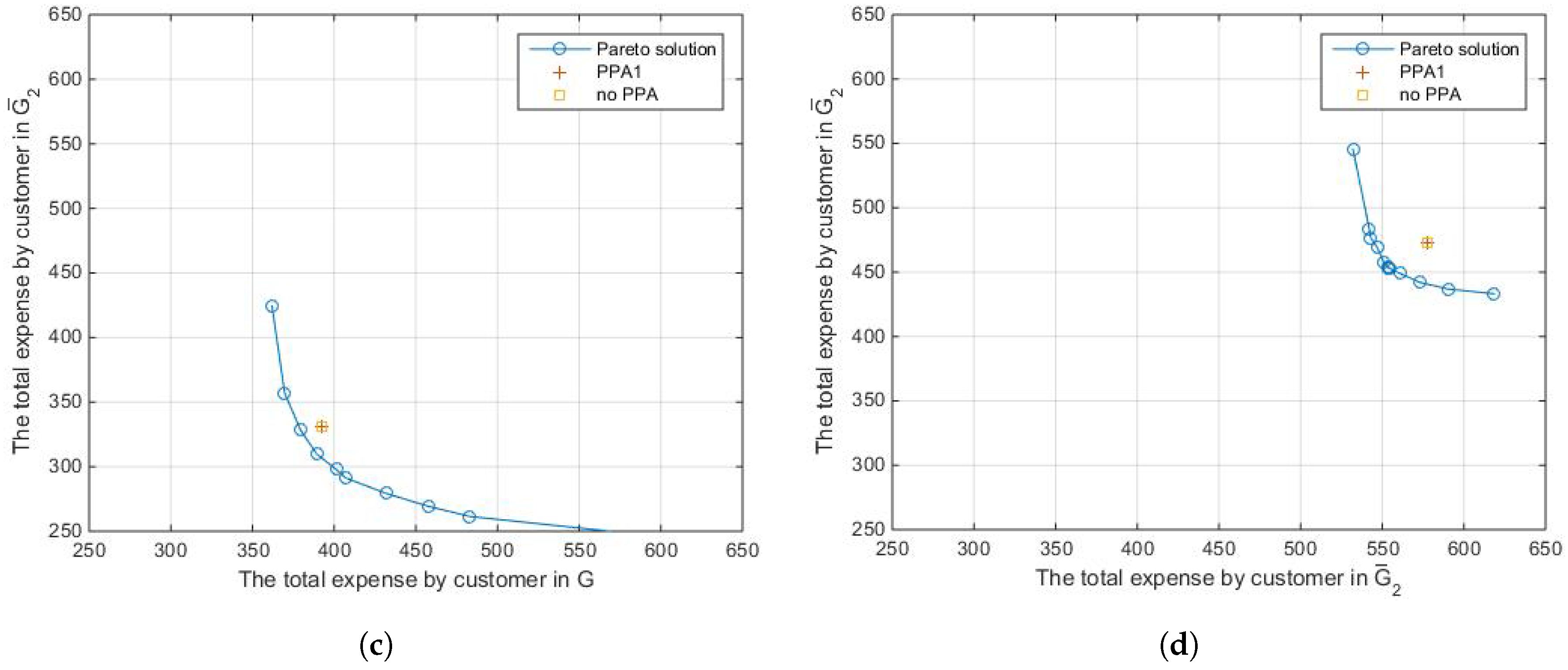
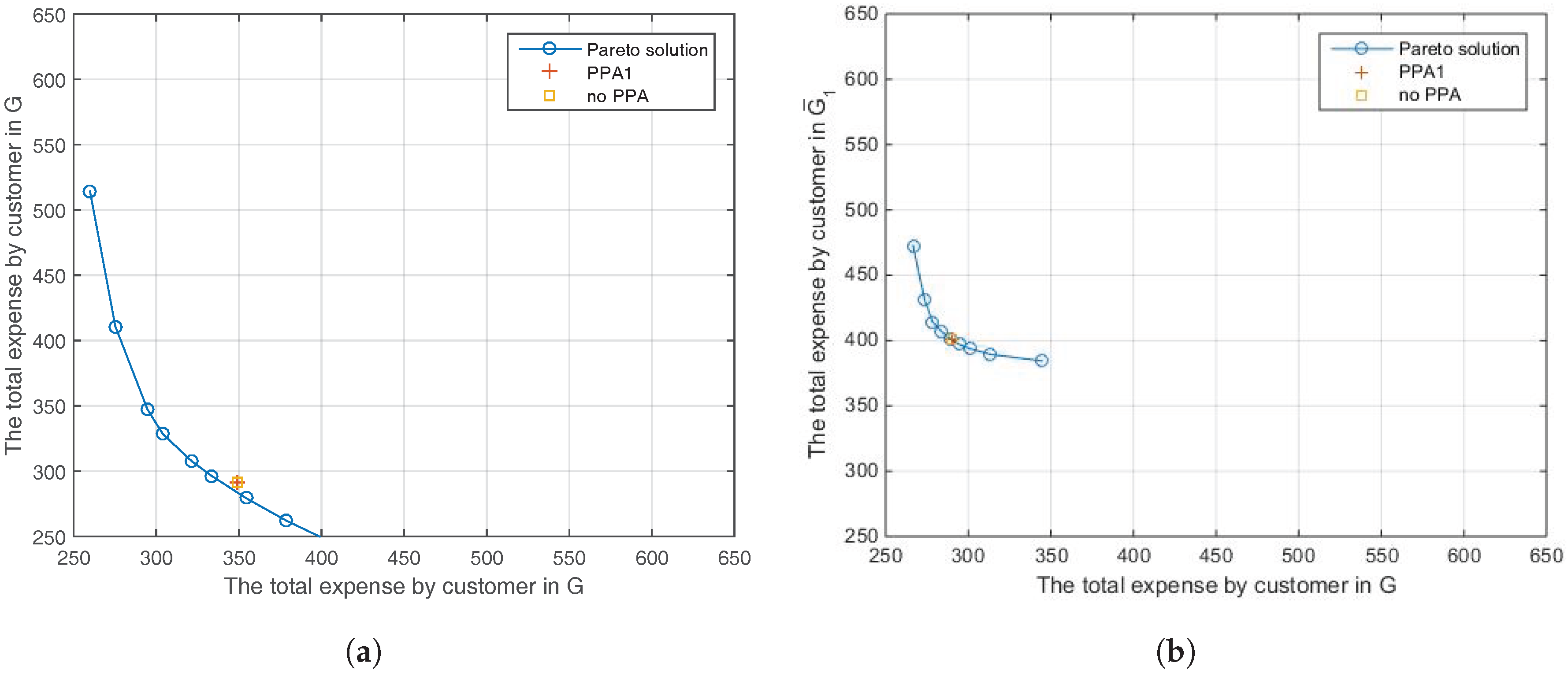
In order to graphically compare solutions from (MP) and (GP) in two-dimensional figures, we consider two-customer problems. Each of the customers is selected from one of the following pairs of customer sets, respectively: (), (), (), () which build four test scenarios. Appliance data from HLM1 and HLM2 are used for the first and the second customer, respectively. That is, the same electricity demand is used in testing four scenarios. We solve the problems by (WMP) with various weights (by taking ) to construct Pareto-optimal trajectories and also by PPA1 and “no PPA” to check whether the game-theoretic solution is Pareto-efficient. In PPA1 and “no PPA”, we use as a termination condition. Figure 8 summarizes the simulation results. In Figure 8a, the results from the () game are shown. With this game, “no PPA” also converges to a solution of PPA1, the expenses of which are exactly matched, and thus, only one point is shown for “no PPA” and PPA1. It is also seen that the game-theoretic solutions are not Pareto-efficient since they are above (worse than) the Pareto trajectory. This means that the expense of a customer resulting from the game-theoretic approaches can be improved without any sacrifice of the other, and thus, some solutions on the Pareto trajectory dominate the game-theoretic solutions. In Figure 8b, results from the () game are shown. In this case, “no PPA” converges to a solution of PPA1, and it is placed on the Pareto trajectory. Especially, the game-theoretic solutions are exactly the same as the Pareto-optimal solution obtained when . In Figure 8c, the results from the () game are shown, where “no PPA” converges to a solution of PPA1, but it is not Pareto-efficient. In Figure 8d, the results from the () game are shown. In this game, the customers have not installed PVS and ESS, where “no PPA” and PPA1 give the same solution, but it is not Pareto-efficient.
By comparing the four figures in Figure 8, it is seen that the () game obtains economically the most efficient solution by both of the customers optimally adjusting PVS and ESS capacities, but the () game provides the worst solution since none of the customers would use PVS and ESS. Figure 8d→Figure 8c→Figure 8a illustrate a path of improvement in the customers’ expenses according to gradually introducing PVS and ESS into smart grids. Especially, by comparing Figure 8c,d, it is seen that the benefit of installing PVS and ESS for one customer could be shared by the other customer that is currently not willing to install the equipment. Specifically, referring to the game-theoretic solution in Figure 8c,d, installation of PVS and ESS by one of the customers (HLM1) changes the expense vector from (578.00, 472.72) to (392.47, 331.26), which reduces nearly 32.10–30% of the expense. If the other customer also wants to be equipped with PVS and ESS, (referring to Figure 8a), the expense further decreases to (348.62, 290.83), which results in a 38.48–39.68% reduction in expense compared with the without-PVS case.
5. Conclusions
In this paper, we have investigated the problem of finding optimal capacities of PV and ES systems in the context of home load management in smart grids. The problem is formulated by two related problems: multi-objective optimization and the game-theoretic approach. The electricity price obtained as a result of individual load management of the customers in the market is autonomously considered in the capacity planning. Solutions from the two approaches are compared, and it is found that the game-theoretic approach cannot converge to or provide, if PPA is used, a Pareto-efficient solution. In our simulation, it is shown to be optimal if 54.52% load is covered by PV and ES systems, for which the expense caused by purchasing the equipment is about 57.48% of the total daily expense of the home considered. Moreover, when a customer optimally decides to install PV and ES systems, the expense of the other customers is also decreasing, by 39.67% in the simulation, since the installation lets the electricity price be reduced. Though the simulation is limited, it is clear that introducing PV and ES systems optimally at a customer can reduce the electricity price and hence diminish the expense of the other customers.
Unlike existing studies on optimal sizing of PV and ES, which have treated it as a part of designing hybrid energy systems or polygeneration systems, our model explicitly considers the varying electricity price that is a result of the individual load management of the customers. Thus, our model can be used to determine more practical sizes of PV and ES in residential environments. We in a future study plan to build up an autonomous and intelligent recommendation module that suggests optimal sizes of PV and ES (hopefully including wind generation) for a specific home connected to more than a thousand other customers. Moreover, we also plan to link the demand-side load management with residential PV and ES systems and the plant operation planning in the nation-wide electricity industry. In this case, the number of customers, including office buildings, factories, as well as homes could be more than tens of millions, which require specific statistical and decomposition methods to be developed.
Acknowledgments
This research was supported by the Korea Ministry of Environment (MOE) as the Climate Change Correspondence Program (201400130001).
Author Contributions
Somi Jung wrote about HLM model and prepared for the simulation and data. Dongwoo Kim wrote about the formulations and investigations.
Conflicts of Interest
The authors declare no conflict of interest.
Abbreviations
The following abbreviations are used in this manuscript:
| SM | Smart meter |
| HLM | Home load management |
| HA | Home appliance |
| PVS | Photovoltaic generation |
| ESS | Energy storage system |
| NTS | Non time-shiftable |
| PS | Power-shiftable |
| TS | Time-shiftable |
| PPA | Proximal point algorithm |
References
- Technology Roadmap: Smart Grids. Available online: https://www.iea.org/publications/freepublications/publication/TechnologyRoadmapSolarPhotovoltaicEnergy_2014edition.pdf (accessed on 6 February 2017).
- Smart Grids: From innovation to Deployment, European Commission; Tech Report; The Commission to the European Parliament, the Council, the European Economic and Social Committee, and the Committee of the Regions: Brussels, Belgium, 12 April 2011.
- Masters, G.M. Renewable and Efficient Electric Power Systems; Wiley: Hoboken, NJ, USA, 2004. [Google Scholar]
- Reducing Electricity Consumption in Houses, Ontario Home Builders’ Assoc.; Energy Conservation Committee Report and Recommendations: Toronto, ON, Canada, 21 April 2006.
- Olivares, D.E.; Merhrizi-Sani, A.; Etemadi, A.H.; Canizares, C.A.; Iravani, R.; Kazerani, M.; Hajimiragha, A.H.; Gomis-Bellmunt, O.; Saeedifard, M.; Palma-Behnke, R.; et al. Trends in microgrid control. IEEE Trans. Smart Grid 2014, 5, 1905–1919. [Google Scholar] [CrossRef]
- Safdarian, A.; Fotuhi-Firuzabad, M.; Lehtonen, M. Optimal residential load management in smart grids: A decentralized framework. IEEE Trans. Smart Grid 2016, 7, 1836–1845. [Google Scholar] [CrossRef]
- Moradzadeh, B.; Tomsovic, K. Two-stage residential energy management considering network operational constraints. IEEE Trans. Smart Grid 2013, 4, 2339–2346. [Google Scholar] [CrossRef]
- Guo, Y.; Pan, M.; Fang, Y.; Khargonekar, P.P. Decentralized coordination of energy utilization for residential households in the smart grid. IEEE Trans. Smart Grid 2013, 4, 1341–1350. [Google Scholar] [CrossRef]
- Atzeni, I.; Ordóñez, L.G.; Scutari, G.; Palomar, D.P.; Fonollosa, J.R. Demand-side management via distributed energy generation and storage optimization. IEEE Trans. Smart Grid 2013, 4, 866–876. [Google Scholar] [CrossRef]
- Zhu, Z.; Chin, W.H. An integer linear programming based optimization for home demand-side management in smart grid. In Proceedings of the 2012 IEEE PES, Innovative Smart Grid Technologies (ISGT), Washington, DC, USA, 16–20 January 2012; pp. 1–5. [Google Scholar]
- Liu, R. An algorithmic game approach for demand side management in smart grid with distributed renewable power generation and storage. Energies 2016, 9, 654. [Google Scholar] [CrossRef]
- Diaf, S.; Notton, G.; Belhamel, M.; Haddadi, M.; Louche, A. Design and techno-economical optimization for hybrid PV/wind system under various meteorological conditions. Appl. Energy 2008, 85, 968–987. [Google Scholar] [CrossRef]
- Koutroulis, E.; Kolokotsa, D.; Potirakis, A.; Kalaitzakis, K. Methodology for optimal sizing of stand-alone photovoltaic/wind-generator systems using genetic algorithms. Sol. Energy 2006, 80, 1072–1088. [Google Scholar] [CrossRef]
- Yang, H.; Zhou, W.; Lu, L.; Fang, Z. Optimal sizing method for stand-alone hybrid solar/wind system with LPSP technology by using genetic algorithm. Sol. Energy 2008, 82, 354–367. [Google Scholar] [CrossRef]
- Dufo-Lopez, R.; Bernal-Agustin, J.L. Design and control strategies of PV-Diesel systems using genetic algorithms. Sol. Energy 2005, 79, 33–46. [Google Scholar] [CrossRef]
- Dufo-Lopez, R.; Bernal-Agustin, J.L.; Yusta-Loyo, J.M.; Domínguez-Navarro, J.A.; Ramírez-Rosado, I.J.; Lujano, J.; Aso, I. Multi-objective optimization minimizing cost and life cycle emissions of stand-alone PV/wind/diesel systems with batteries storage. Appl. Energy 2011, 88, 4033–4041. [Google Scholar] [CrossRef]
- Chen, H.-C. Optimum capacity determination of stand-alone hybrid generation system considering cost and reliability. Appl. Energy 2013, 103, 155–164. [Google Scholar] [CrossRef]
- Zhao, B.; Zhang, X.; Li, P.; Wang, K.; Xue, M.; Wang, C. Optimal sizing, operating strategy and operational experience of a stand-alone microgrid on Dongfushan Island. Appl. Energy 2014, 113, 1656–1666. [Google Scholar] [CrossRef]
- Perera, A.T.D.; Attalage, R.A.; Perera, K.K.C.K.; Dassanayake, V.P.C. A hybrid tool to combine multi-objective optimization and multi-criterion decision making in designing standalone hybrid energy systems. Appl. Energy 2013, 107, 412–425. [Google Scholar] [CrossRef]
- Nosrat, A.; Pearce, J.M. Dispatch strategy and model for hybrid photovoltaic and trigeneration power systems. Appl. Energy 2011, 88, 3270–3276. [Google Scholar] [CrossRef]
- Rubio-Maya, C.; Uche-Marcuello, J.; Martínez-Gracia, A.; Bayod-Rújula, A.A. Design optimization of a polygeneration plant fuelled by natural gas and renewable energy sources. Appl. Energy 2011, 88, 449–457. [Google Scholar] [CrossRef]
- Wang, J.; Zhai, Z.; Jing, Y.; Zhang, C. Particle swarm optimization for redundant building cooling heating and power system. Appl. Energy 2010, 87, 3668–3679. [Google Scholar] [CrossRef]
- Ko, M.J.; Kim, Y.S.; Chung, M.H.; Jeon, H.C. Multi-objective optimization design for a hybrid energy system using the genetic algorithm. Energies 2015, 8, 2924–2949. [Google Scholar] [CrossRef]
- Hernandez-Aramburo, C.A.; Green, T.C.; Mugniot, N. Fuel consumption minimization of a microgrid. IEEE Trans. Ind. Appl. 2005, 41, 673–681. [Google Scholar] [CrossRef]
- Varaiya, P.P.; Wu, F.F.; Bialek, J.W. Smart operation of smart grid: Risk-limiting dispatch. IEEE Proc. 2011, 99, 40–57. [Google Scholar] [CrossRef]
- Ontario Bill 150, Green Energy and Green Economy Act, 2009. Available online: http://www.ontla.on.ca/web/bills/bills_detail.do?BillID=2145 (accessed on 6 February 2017).
- Recent Facts about Photovoltaics in Germany. Available online: https://www.ise.fraunhofer.de/content/dam/ise/en/documents/publications/studies/recent-facts-about-photovoltaics-in-germany.pdf (accessed on 6 February 2017).
- Mohsenian-Rad, A.-H.; Wong, V.W.S.; Jatskevich, J.; Schober, R.; Leon-Garcia, A. Autonomous demand-side management based on game-theoretic energy consumption scheduling for the future smart grid. IEEE Trans. Smart Grid 2010, 1, 320–331. [Google Scholar] [CrossRef]
- Rockafellar, R.T. Monotone operators and the proximal point algorithm. SIAM J. Control Optim. 1976, 14, 877–898. [Google Scholar]
- Bracale, A.; Pierluigi, C.; Guido, C.; Anna, R.D.F.; Gabriella, F. A Bayesian method for short-term probabilistic forecasting of photovoltaic generation in smart grid operation and control. Energies 2013, 6, 733–747. [Google Scholar] [CrossRef]
- Duffie, J.A.; Beckman, W.A. Solar Engineering of Thermal Processes; John Wiley & Sons: Hoboken, NJ, USA, 2013. [Google Scholar]
- Pareto, V. Cours d’ Economie Politique, Rouge, Lausanne, 1897. Reprinted as the First Volume of Oeuvres Completes; Droz: Geneva, Switzerland, 1964. [Google Scholar]
- Chankong, V.; Haimes, Y.Y. Multiobjective Decision Making: Theory and Methodology; Courier Dover Publications: Mineola, NY, USA, 2008. [Google Scholar]
- Parikh, N.; Boyd, S. Proximal algorithms. Found. Trends Optim. 2014, 1, 127–239. [Google Scholar] [CrossRef]
Figure 1.
Smart grid model.

Figure 2.
Hourly capacity factor of PV generation.
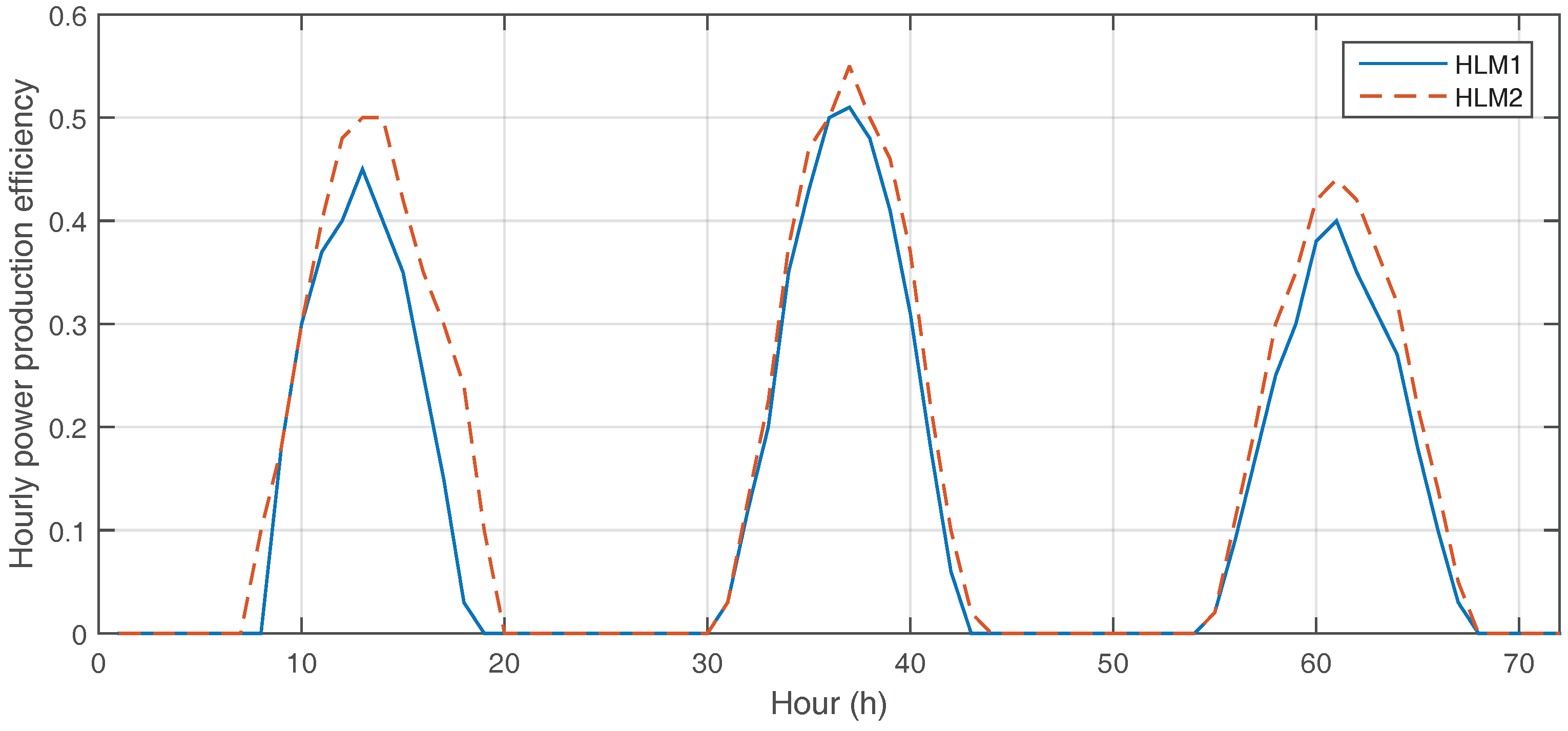
Figure 3.
Optimal capacities of PVS and ESS and the resulting expenses from multi-objective optimization. (a) Optimal capacities of PVS and ESS; (b) individual and average expenses resulting from optimal installation of PVS and ESS.
Figure 3.
Optimal capacities of PVS and ESS and the resulting expenses from multi-objective optimization. (a) Optimal capacities of PVS and ESS; (b) individual and average expenses resulting from optimal installation of PVS and ESS.


Figure 4.
Per-hour electricity price and load profile with and without PVS and ESS in HLM1 from multi-objective optimization. (a) Electricity price with and without PVS and ESS in HLM1; (b) per-hour total load profile with and without PVS and ESS in HLM1.
Figure 4.
Per-hour electricity price and load profile with and without PVS and ESS in HLM1 from multi-objective optimization. (a) Electricity price with and without PVS and ESS in HLM1; (b) per-hour total load profile with and without PVS and ESS in HLM1.


Figure 5.
PV generation and ES profile from multi-objective optimization. (a) PV generation profile; (b) ES charging, discharging and storage profile.
Figure 5.
PV generation and ES profile from multi-objective optimization. (a) PV generation profile; (b) ES charging, discharging and storage profile.
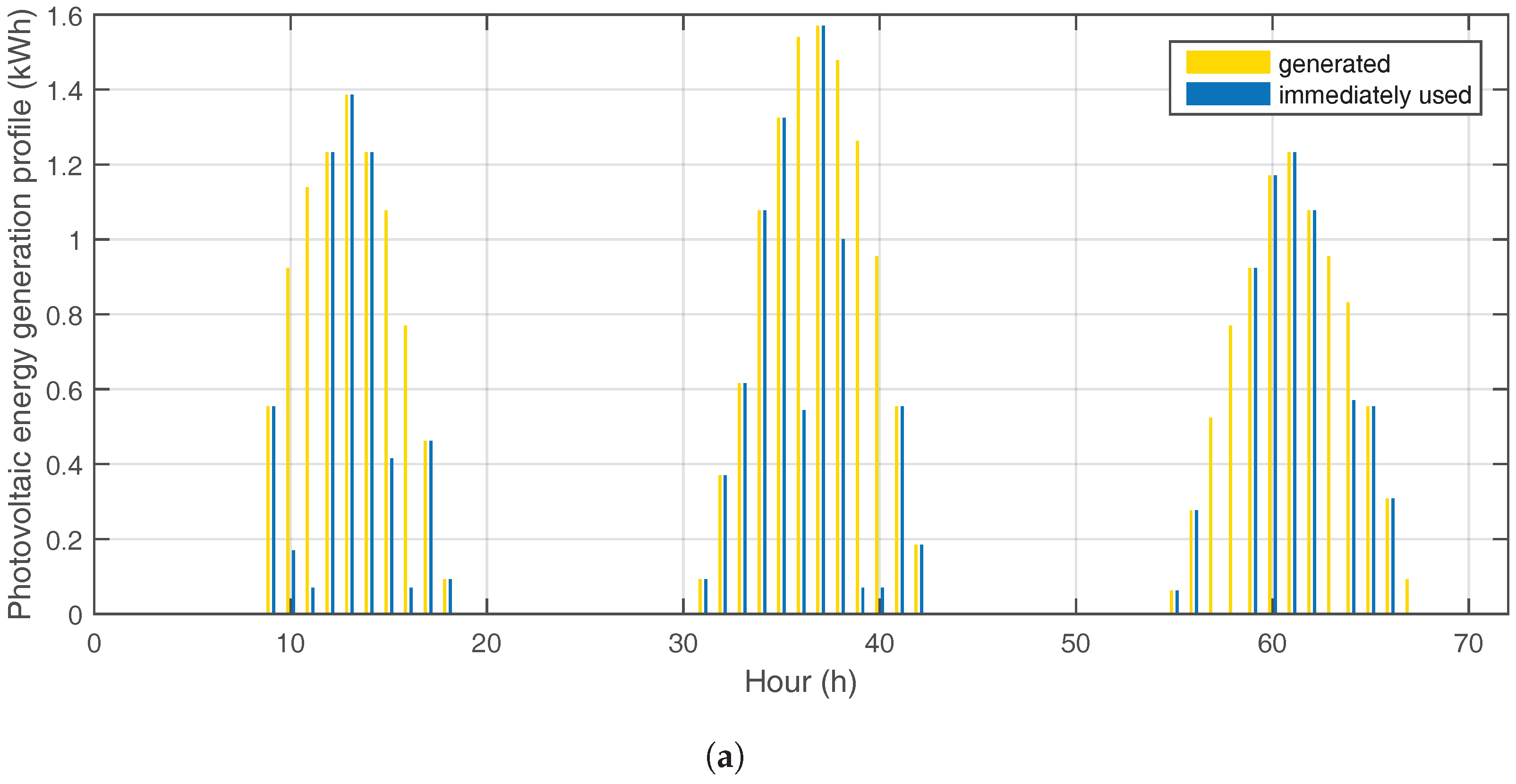
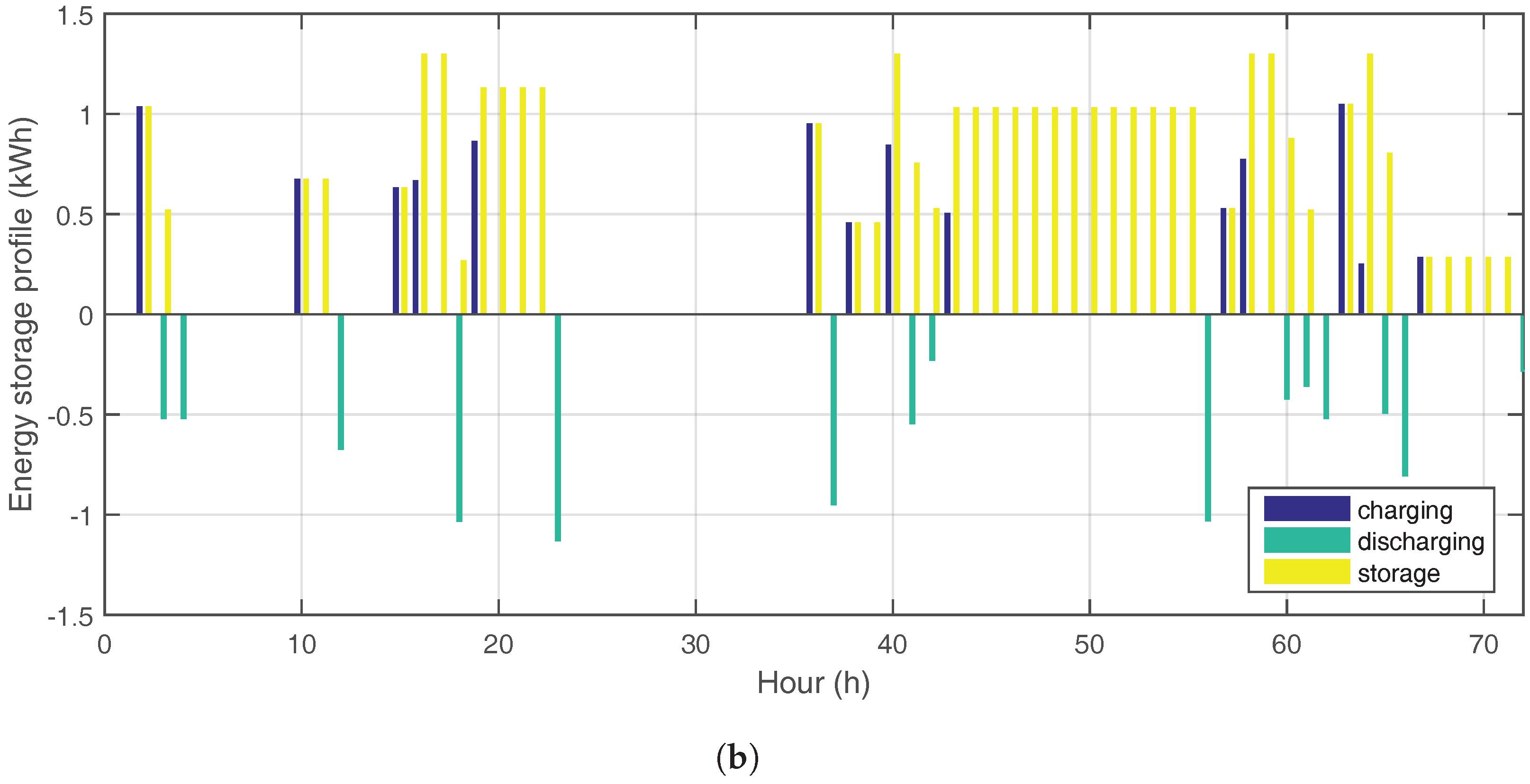
Figure 6.
Convergence behavior of game-theoretic approaches. (a) Comparison of updating distances by PPA1, PPA2 and “no PPA”; (b) comparison of updating expenses by PPA2 and “no PPA”.
Figure 6.
Convergence behavior of game-theoretic approaches. (a) Comparison of updating distances by PPA1, PPA2 and “no PPA”; (b) comparison of updating expenses by PPA2 and “no PPA”.

Figure 7.
Total load per hour from the game-theoretic solution of PPA1.
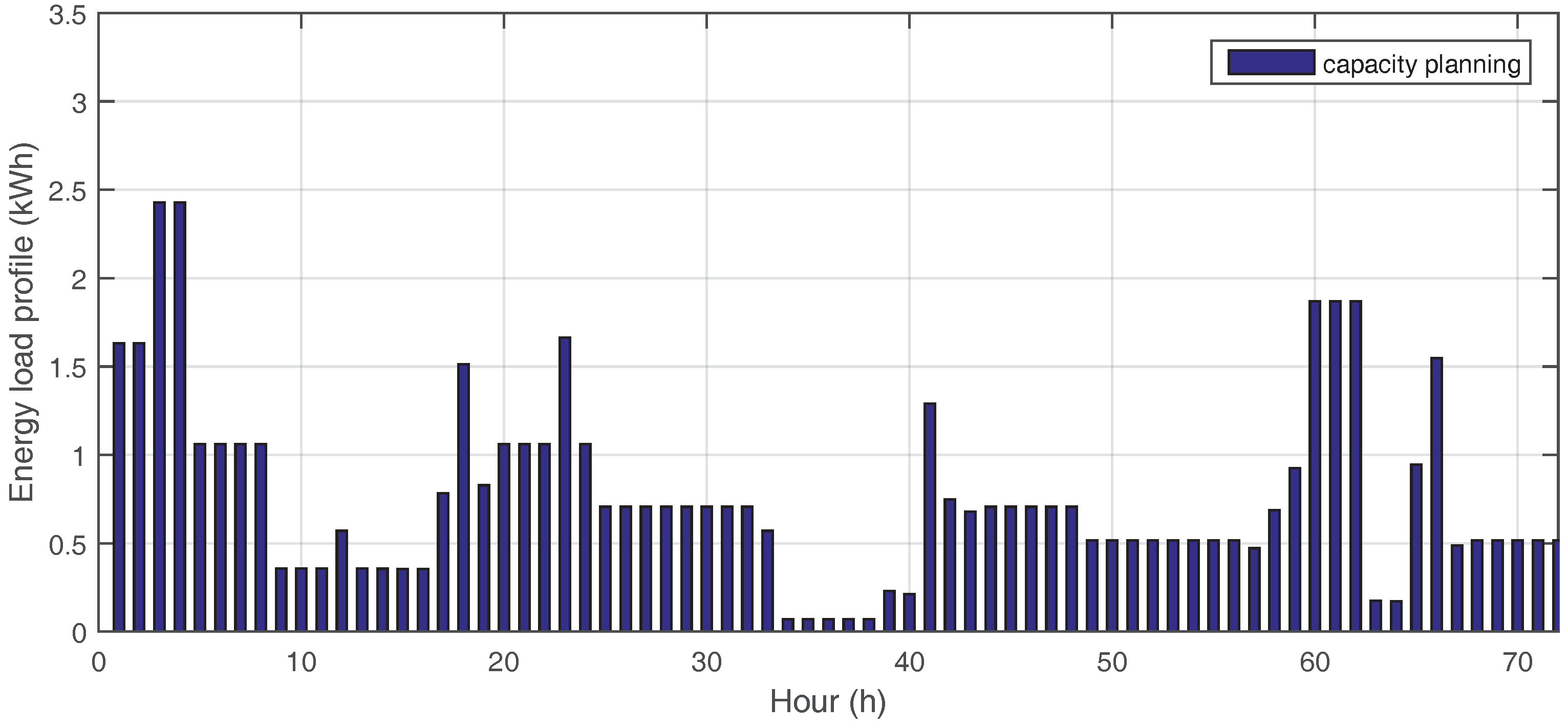
Figure 8.
Pareto-efficient vs. game-theoretic solutions from four scenarios of comparison. (a) () game; (b) () game; (c) () game; (d) () game.
Figure 8.
Pareto-efficient vs. game-theoretic solutions from four scenarios of comparison. (a) () game; (b) () game; (c) () game; (d) () game.


Table 1.
Notations for sets, parameters and variables. PVS, photovoltaic system; ESS, energy storage system.
Table 1.
Notations for sets, parameters and variables. PVS, photovoltaic system; ESS, energy storage system.
| Type | Symbol | Definition |
|---|---|---|
| Sets | set of customers in the power system | |
| set of customers that are willing to install PVS and ESS at their home | ||
| set of customers that are already equipped with PVS and ESS | ||
| set of customers that currently do not consider PVS and ESS | ||
| set of household appliances at customer n | ||
| Parameters | daily price profile at hour h. | |
| unit cost of installing PVS by customer n | ||
| unit cost of installing ESS by customer n | ||
| r | market rate of interest per day | |
| hourly power production efficiency of PVS installed by customer n | ||
| PV capacity installed by customer n at hour h | ||
| ES capacity installed by customer n at hour h | ||
| leakage rate of ES installed by customer n | ||
| charging efficiency of ES installed by customer n | ||
| discharging efficiency of installed by customer n | ||
| daily electricity requirement of appliance a at customer n | ||
| fixed energy requirement of appliance a at customer n | ||
| standby power of appliance a at customer n | ||
| maximum working power of appliance a at customer n | ||
| fixed energy consumption pattern of appliance a at customer n | ||
| matrix of standby power of appliance a at customer n | ||
| matrix of maximum working power of appliance a at customer n | ||
| Variables | energy load profile by customer n at hour h | |
| electricity requirement due to charging ESS by customer n at hour h | ||
| PV energy generation profile by customer n at hour h | ||
| energy generated by PV at hour h and immediately used at that time slot in customer n | ||
| energy storage profile of customer n at hour h | ||
| energy charging profile of customer n at hour h | ||
| energy discharging profile of customer n at hour h | ||
| PV capacity installed by customer n | ||
| ES capacity installed by customer n | ||
| energy consumption scheduling of appliance a in customer n at hour h | ||
| binary variable indicating switch control for the time-shiftable appliances |
Table 2.
Notations for the constraint set.
| Notation | Constraint | Index Set | |
|---|---|---|---|
| . | a ∈ | ||
| . | |||
| , = 0 or 1. | |||
| . | n ∈ | ||
| 0. | |||
| n | |||
| n | |||
Table 3.
Proximal point algorithm (PPA).
| Step 0. | Set and an initial reference solution |
| Find any initial feasible starting point . Set and . | |
| Step 1. | For , each customer computes such that |
| subject to the constraints in (22). | |
| Step 2. | If a Nash equilibrium is reached, go to Step 3. Otherwise, update and go to Step 1. |
| Step 3. | If , then terminate. |
| Otherwise, update for , and . And go to Step 1. |
Table 4.
Appliance and power consumption pattern (unit : kWh, hour).
| Appliance | HLM1 | HLM2 | HLM3 | ||||
|---|---|---|---|---|---|---|---|
| Class | Type | Consumption Requirement | Time Period | Consumption Requirement | Time Period | Consumption Requirement | Time Period |
| NTS | Hob and oven | 1.0(H) | 17–18 | 1.0(H) | 17–18 | 1.2(H) | 18 |
| Heater | 1.0(H) | 3–4, 23 | 1.0(H) | 3–4, 23 | 1.5(H) | 3–4, 23 | |
| Fridge and freezer | 0.07(H) | 24 h | 0.07(H) | 24 h | 0.07(H) | 24 h | |
| Air conditioner | 1.5(H) | 11–14 | 1.55(H) | 11–14 | 1.5(H) | 12–14 | |
| PS | Water boiler | 0–1.2, 2(D) | 24 h | 0–1.5, 2(D) | 24 h | 0–1.2,2(D) | 24 h |
| Electric fan | 0–0.07, 0.7(D) | 24 h | 0–0.07, 0.8(D) | 24 h | 0–0.07, 0.8(D) | 24 h | |
| Electric vehicle | 0–3.5(D) | 20–8 | 0–2.3(D) | 20–8 | - | - | |
| TS | Washing machine | 0.5(H) | 1 h /day | 0.5(H) | 1 h/day | 0.5(H) | 1 h/day |
| TV | 0.1, 0.15(H) | 2 h/day | 0.1, 0.15(H) | 2 h/day | - | - | |
| Dishwasher | 1.8(H) | 1 h/day | - | - | - | - | |
© 2017 by the authors. Licensee MDPI, Basel, Switzerland. This article is an open access article distributed under the terms and conditions of the Creative Commons Attribution (CC BY) license (http://creativecommons.org/licenses/by/4.0/).
Share and Cite
MDPI and ACS Style
Jung, S.; Kim, D. Pareto-Efficient Capacity Planning for Residential Photovoltaic Generation and Energy Storage with Demand-Side Load Management. Energies 2017, 10, 426. https://doi.org/10.3390/en10040426
AMA Style
Jung S, Kim D. Pareto-Efficient Capacity Planning for Residential Photovoltaic Generation and Energy Storage with Demand-Side Load Management. Energies. 2017; 10(4):426. https://doi.org/10.3390/en10040426
Chicago/Turabian StyleJung, Somi, and Dongwoo Kim. 2017. "Pareto-Efficient Capacity Planning for Residential Photovoltaic Generation and Energy Storage with Demand-Side Load Management" Energies 10, no. 4: 426. https://doi.org/10.3390/en10040426
Note that from the first issue of 2016, this journal uses article numbers instead of page numbers. See further details here.