
Predictive Direct Flux Control—A New Control Method of Voltage Source Inverters in Distributed Generation Applications


Department of Electrical Engineering, The Hong Kong Polytechnic University, Hong Kong, China
Energies 2017, 10(4), 428; https://doi.org/10.3390/en10040428
Submission received: 16 February 2017
/
Revised: 21 March 2017
/
Accepted: 21 March 2017
/
Published: 23 March 2017
Abstract
:Voltage source inverters (VSIs) have been widely utilized in electric drives and distributed generations (DGs), where electromagnetic torque, currents and voltages are usually the control objectives. The inverter flux, defined as the integral of the inverter voltage, however, is seldom studied. Although a conventional flux control approach has been developed, it presents major drawbacks of large flux ripples, leading to distorted inverter output currents and large power ripples. This paper proposes a new control strategy of VSIs by controlling the inverter flux. To improve the system’s steady-state and transient performance, a predictive control scheme is adopted. The flux amplitude and flux angle can be well regulated by choosing the optimum inverter control action according to formulated selection criteria. Hence, the inverter flux can be controlled to have a specified magnitude and a specified position relative to the grid flux with less ripples. This results in a satisfactory line current performance with a fast transient response. The proposed predictive direct flux control (PDFC) method is tested in a 3 MW high-power grid-connected VSI system in the MATLAB/Simulink environment, and the results demonstrate its effectiveness.
1. Introduction
Pulse width modulation (PWM) voltage source inverters (VSIs) have been widely used in power electronics, and their control has been extensively studied in the last decades. One of the most popular applications of VSIs is electric drives for speed control and electromagnetic torque regulation [1]. Recently, inverter-interfaced distributed generation (DG) systems (wind turbines, photovoltaic (PV), wave generators, etc.) have raised concern. These DGs are either connected to a common bus to form a small isolated power system, or connected to the main utility grid. The power supplied by the DGs as well as the DG output voltage and current can be flexibly regulated by controlling VSIs in various operation conditions [2,3].
In the VSI applications mentioned above, generally two individual quantities are controlled in closed-loop strategies for inverters by means of switching. Traditionally the d- and q-axis current components are directly controlled in electric drives [4]. Later on, direct torque control (DTC) was proposed and it eliminates the need for a current regulator and provides direct control of the motor electromagnetic torque [5]. Derived from DTC, direct power control (DPC) was proposed to control rectifiers and inverters by using the active and reactive powers as control variables in DGs [6]. Similarly, direct current control and direct voltage control were proposed for grid-connected or isolated VSI systems [7,8].
However, the torques (or active and reactive powers, currents and voltages) are not the only quantities that can be regulated directly by the inverter switching. The control of the inverter flux has raised concern in the last few years because the inverter flux is less sensitive to external disturbance for its voltage integral feature [9,10,11]. Inverter flux control was first proposed by Chandorkar et al. [9,10] for inverter stand-alone operations. Nevertheless, it has not been applied in grid-connected inverters. Inverter flux was adopted in grid-connected converters [11]. However, the inverter flux was just used to estimate the active and reactive powers in order to eliminate the instantaneous errors during measurement. In other words, the direct control variables of the inverters are active and reactive powers rather than the inverter flux. To the best of the authors’ knowledge, there are no existing papers working on direct flux control for grid-connected VSI systems. In addition, the magnitude of the inverter flux is related to the inverter voltage while the position of the inverter flux links to the voltage frequency. Therefore, inverter flux control could be a promising alternative for grid-connected renewable energy systems to performance grid support. Unfortunately, the existing inverter flux control strategies are still under development. The only approach reported in the literature is the switching table–based direct flux control, or SDFC [9,10]. In this scheme, the inverter switching is selected from a predefined switching table according to the position of the inverter flux. As a result, similar to conventional DTC and DPC, large flux ripples are the main drawback of SDFC. This leads to deteriorated power and current quality.
In order to address the disadvantages of SDFC, a new inverter control method is proposed in this paper by adopting predictive control to the inverter flux concept. The controller uses the system model and all the possible switching states to predict the behavior of the inverter flux, namely the flux amplitude and the flux position, at the next sampling instant. Then, a cost function is employed as a criterion to evaluate the inverter flux performance. Finally, the voltage vector or the switching state that minimizes the cost function will be applied during the next sampling interval. In this way, the inverter flux can be well controlled to track the reference. Also, it is necessary to point out that the proposed method in this paper falls into the category of model predictive control (MPC), while the method presented in [11] belongs to the category of vector sequence–based predictive control. The cost function developed here presents totally different meanings to the cost function described in [11]. In our work, the optimal voltage vector is selected according to the cost function, whereas the voltage vector sequences are selected according to a predefined switching table. The cost function is used to calculate the applied duration of the selected voltage vectors.
The rest of this paper is organized as follows. The VSI system configuration and the inverter flux concept are described in Section 2. The conventional SDFC method is presented in Section 3, while the new predictive direct flux control (PDFC) is introduced in Section 4. The effectiveness of the proposed method is verified in Section 5. The conclusion is presented in Section 6.
2. Flux Concept in VSI Systems
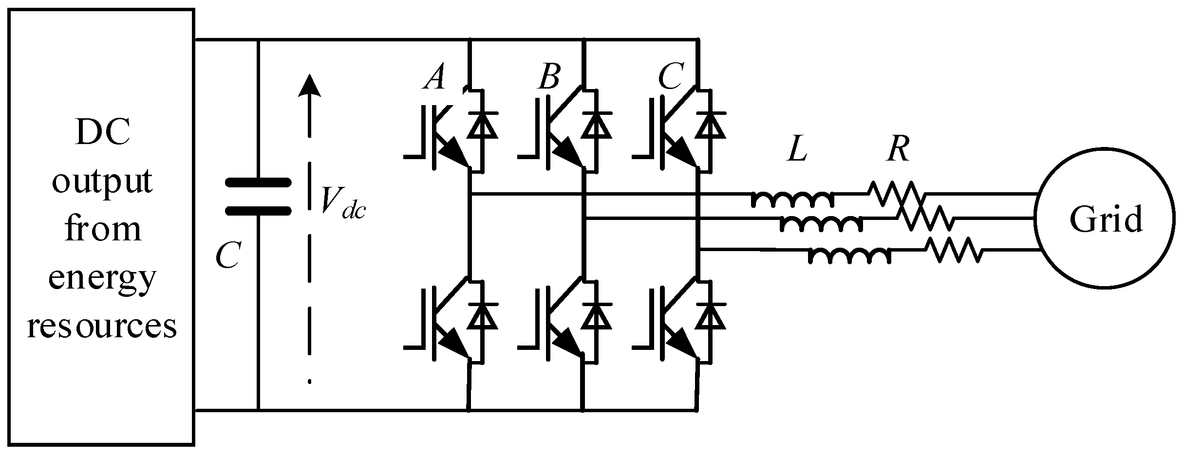
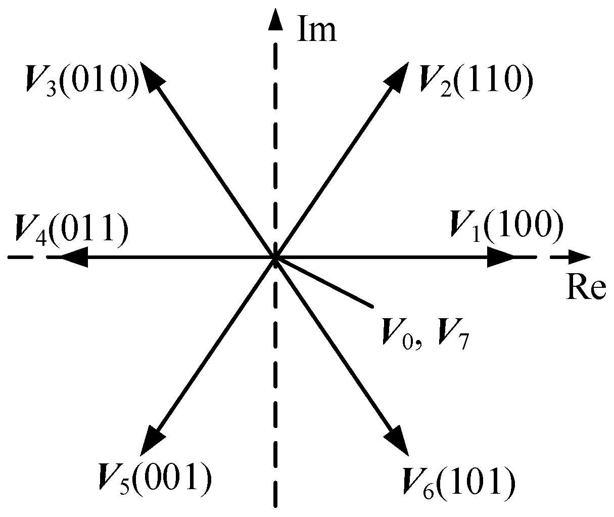
The power circuit considered is shown in Figure 1. The energy resources are interfaced with the grid through the three-phase two-level VSI with six insulated gate bipolar transistors (IGBTs). The DC output from the energy resources could be from the solar PV panels, the permanent magnet synchronization wind generator with diode rectifiers, etc. L and R represent the line inductor and resistor, respectively. Depending on the switching states, the inverter can be controlled to generate eight possible output voltages including six active vectors and two null vectors. They can be expressed in complex space vectors as:
where Vdc is the dc-link voltage. Figure 2 shows the inverter output voltages in terms of amplitude and position in the stationary α-β frame. For instance, if the upper switches of phases A and B are turned ON while the upper switch of phase C is turned OFF, voltage vector V2 with an amplitude of 2/3 Vdc and a phase angle of 60° will be generated. It is noted that this two-dimensional plane can be divided into six sections, which will be explained and used in inverter flux control. The mathematical equations of the system equivalent circuit can be described as:
where E and I are the grid voltage vector and the line current vector, respectively. R is the line resistance, and L is the line inductance. P and Q are the active and reactive power flow between the system and the utility grid. Similar to the flux definition in an electrical machine, the inverter flux vector and the grid flux vector can be defined as [10]:
It is noted that the inverter flux and the grid flux are the rotating space vectors with a specified amplitude and angular speed. Here, the angle between ΨV and ΨE, indicated as the power angle, is defined as:
where δV and δE are the angles of ΨV and ΨE, respectively.
3. Conventional Switching Table–Based Direct Flux Control (SDFC)
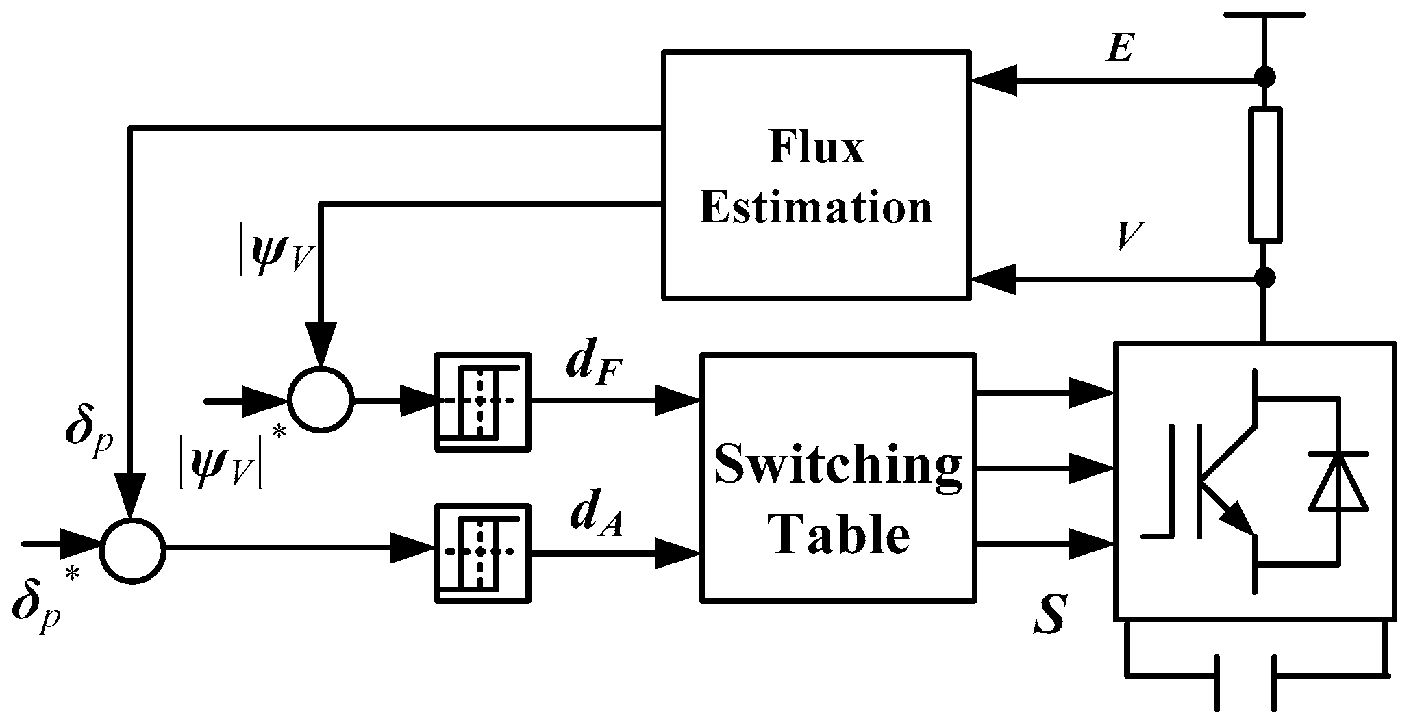
Control of the flux vector has been found to show a good dynamic response and robustness. In conventional SDFC, two variables that are controlled directly by the inverter are |ΨV| and δp. In other words, the vector ΨV is controlled to have a specified magnitude and a specified position relative to the vector ΨE, as shown in Figure 3. The control strategy of the SDFC is depicted in Figure 4. The signals dF and dA are first generated by two hysteresis comparators according to the tracking errors between the estimated and referenced values of the flux and power angle. The voltage vector is then selected from a look-up table (Table 1) according to dF, dA and δV. Similar to the switching table–based DTC and DPC, the SDFC strategy is based on the fact that the effects of each inverter voltage vector on |ΨV| and δ are different. This is summarized in Table 1 [9], where Sk is the sector number in the α-β plane given by the position of ΨV, being dF = 1 if |ΨV|* > |ΨV|, dF = 0 if |ΨV|* < |ΨV|; and dA = 1 if δ* > δ, dA = 0 if δ* < δ.
For instance, assuming that at the kth sampling instant, ΨV is within sector S1, |ΨV|* > |ΨV| and > δ, so that dF = 1 and dA = 1. Therefore, V2(110) will be selected to increase both |ΨV| and δp. After that, V2(110) will be applied during the kth and (k + 1)th sampling instants. In a similar manner to DTC and DPC, this voltage vector can be generated simply by turning on the upper switches and turning off the lower switches of the inverter legs of phases A and B, while turning off the upper switch and turning on the lower switch of phase C. In this way, ΨV is controlled around an approximate circular path within specified hysteresis bands through the inverter switching, which will be demonstrated in the test results.
4. Predictive Direct Flux Control
As explained before, in SDFC, the position of the inverter flux is identified according to an α-β plane divided into six sectors. There is one voltage vector and only that one selected within a whole sector. In fact, the vector selected according to the switching table is not necessarily the best one for controlling the inverter flux amplitude and power angle, especially when the inverter flux position is located near the edge of the sectors. Therefore, it is expected that the voltage vectors are always chosen according to some specified criteria regardless of the inverter flux position.
Based on the above discussion, a PDFC is proposed for VSIs in this paper. In fact, several kinds of control schemes have been developed under the name of predictive control, such as deadbeat predictive control, hysteresis-based predictive control, trajectory-based predictive control, MPC, etc. Due to its flexible control scheme that allows the easy inclusion of system constraints and nonlinearities of the system, MPC has raised much concern in the last few years [12,13]. In MPC, different definitions of the cost function are possible, considering different norms and including several variables and weighting factors [14,15,16]. Taking the advantages of MPC, a new PDFC strategy is developed. Different from the use of hysteresis comparators and the switching table in SDFC, the selection of voltage vectors of the proposed PDFC is based on evaluating a defined cost function.
Generally, the proposed controller consists of three main steps, namely flux prediction, optimal voltage vector selection and weighting factor tuning, as illustrated in Figure 5.
Step 1: Flux prediction
The system variables that need to be predicted are the inverter flux amplitude |ΨV| and the power angle δp. According to Equation (5), we have = + VTs, where Ts is the sampling period and V is the possible inverter voltage vectors. As explained before, V can be controlled to eight space voltage vectors, depending on the switching states. The inverter flux vector can be predicted using α and β components as:
Subsequently, the inverter flux amplitude at the next (k + 1)th sampling instant can be expressed as:
For the inverter flux angle, it can be predicted by:
Since the grid is a stiff AC power system, the grid voltage vector rotates at a constant angular speed. Therefore, the grid flux angle can be simply predicted as:
where ω is the angular speed of the grid voltage in radians per second, i.e., the angular speed of the grid flux. Now that the future states of the inverter flux angle and the grid flux angle have been obtained, the power angle can thus be calculated as:
Substitute Equations (12) and (13) into Equation (8), and the vector that produces the minimum J will be selected to control |ΨV| and δp.
Step 2: Optimal inverter voltage vector selection
After the future behavior of the system is predicted, the next step is to design a cost function (or selection criteria) to evaluate all the possible switching states. Actually, different formulations of the cost function are possible, depending on which variables need to be controlled [15]. In this paper, the cost function is chosen in such a way that both the flux and angle are as close as possible to the referenced values, which is defined as:
where k1 and k2 are the weighting factors, |ΨV|* and are the referenced inverter flux amplitude and power angle, respectively. In this paper, weighting factors are obtained with the purpose of getting a trade-off between the flux and power angle. As there are eight possible voltage vectors, there will be eight possible values of the cost function. Next, the voltage vector that can minimize the cost function will be selected to control the inverter.
Step 3: Weighting factor determination
In grid-connected inverters where active power and reactive power are the control objectives, the weighting factors of the cost function can be decided in a simple way by equalizing k1 and k2, because the active power and reactive power show the same control priority and they have the same order of magnitude. However, the control objectives in this paper are the flux magnitude |ΨV| and the power angle δp. The first term in Equation (14) reduces the flux ripples, while the second term contributes to power angle ripple reduction. For example, a larger value for k1 implies a higher priority for the flux regulation. Now it can be seen that the unit of |ΨV| is Webers while the unit of the δp is radians, and they show different orders of magnitude. Therefore, it is necessary to design a suitable weighting factor determination approach in this case. Here, a two-step tuning method is developed. In coarse tuning, the preliminary ratio of k1/k2 can be obtained according to the nominal values of the power angle and the flux. For instance, if the nominal power angle is 0.7 radians and the nominal flux amplitude is 12 Wb for a grid-connected inverter, then k1:k2 can be set as 0.7:12. In this way, both the flux and the power angle can be controlled in a balance. After that, k1 and k2 will be adjusted slightly in fine tuning until a satisfactory performance is obtained. Actually there is some specified research focused on weighting factor optimization [17,18]. However, the topic of weighting factor optimization is out of the scope of this paper.
5. Results and Discussion
The proposed PDFC of inverters is tested in a 3 MW high-power VSI system connected to 3.3 kV grid in a MATLAB Simulink (MATLAB 2016a, www.mathworks.com) environment. The power circuit of the system is shown in Figure 1. The parameters of the VSI system are listed in Table 2. To demonstrate the effectiveness of the proposed PDFC scheme for VSIs, the conventional SDFC will be employed for comparison. For SDFC, the band width of the hysteresis comparators of the flux magnitude and power angle are HF = 0.075 and HA = 0.01. For PDFC, the weighting factors are k1 = 1, k2 = 18. The sampling rate for both strategies is 10 kHz, leading to a 2.02 kHz average switching frequency for SDFC and a 1.95 kHz average switching frequency for PDFC.
5.1. Steady-State Performance
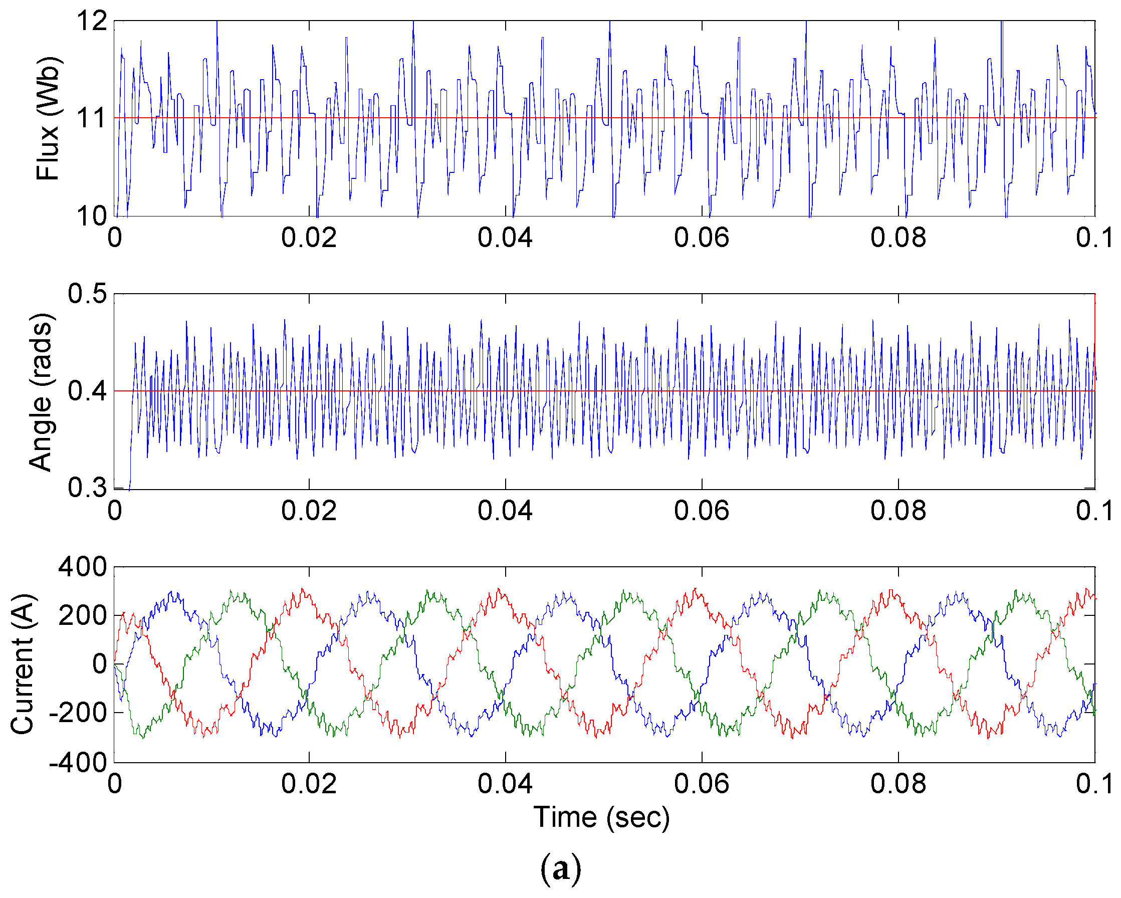
The system steady-state performance is shown in Figure 6. From top to bottom, the curves are the inverter flux magnitude, power angle, and inverter output line currents, respectively. The referenced values of the inverter flux magnitude and power angle are set to 11 Wb and 0.4 rads, respectively. It can be seen that by controlling the VSI with SDFC, both the inverter flux amplitude and power angle present a large amount of oscillations and ripples, though they can track their references roughly. Hence the line currents, i.e., the currents flowing from the DG to the grid, are seriously distorted. As explained previously, these are the main disadvantages of the conventional inverter flux control because the voltage vector applied in every sampling period is not necessarily the most effective one. For grid-tied DG systems, the injected currents should be as sinusoidal as possible. Otherwise, the power quality will be deteriorated by such distorted current components. Consequently, the grid stability will be affected, and additional power losses will be produced. On the other hand, after using the proposed PDFC, it can be observed that the flux amplitude and power angle are much better controlled with a significant ripple reduction. In addition, the line currents are also more sinusoidal than those of SDFC.
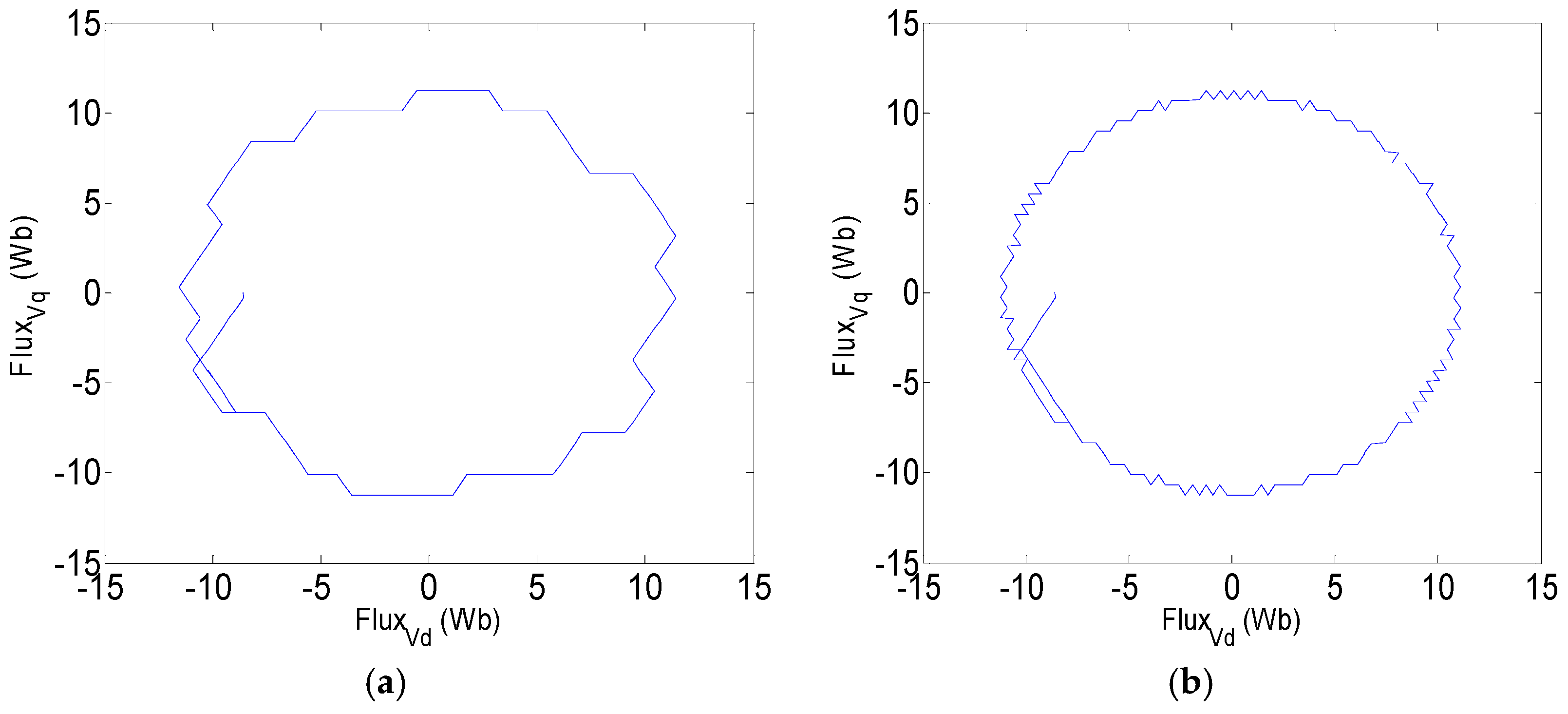
To further demonstrate the better performance of PDFC, Figure 7 shows the locus of the inverter flux vector ΨV. The horizontal axis represents the α component of the inverter flux vector while the vertical axis represents the β component of the inverter flux vector. It is clearly seen that, compared with SDFC, the tip of the inverter flux vector of PDFC is closer to a circle. While the aim of inverter flux control is to enable the inverter flux ΨV to have a specified magnitude and a specified position relative to the grid flux ΨE, PDFC shows better ability in regulating |ΨV| and δp than SDFC.
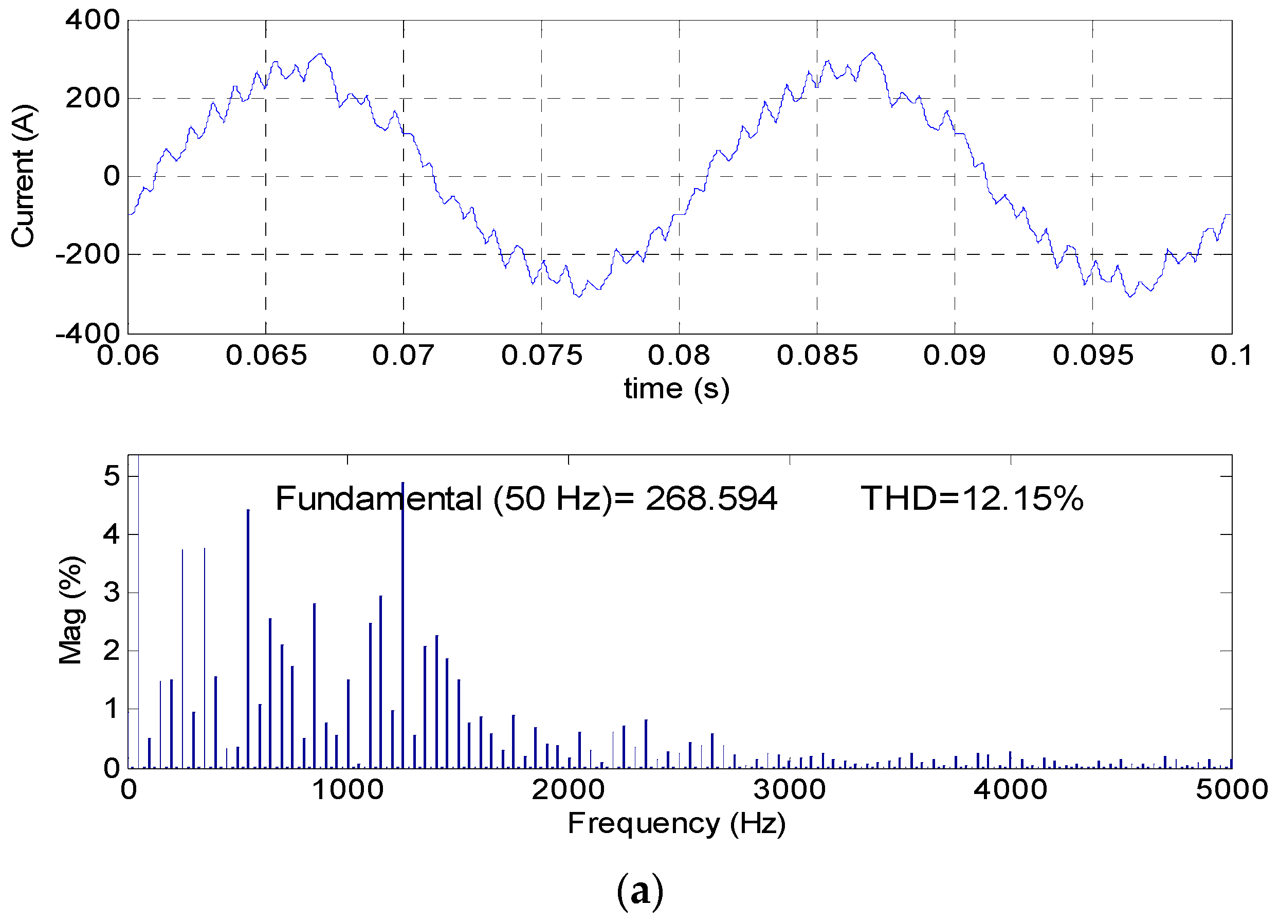
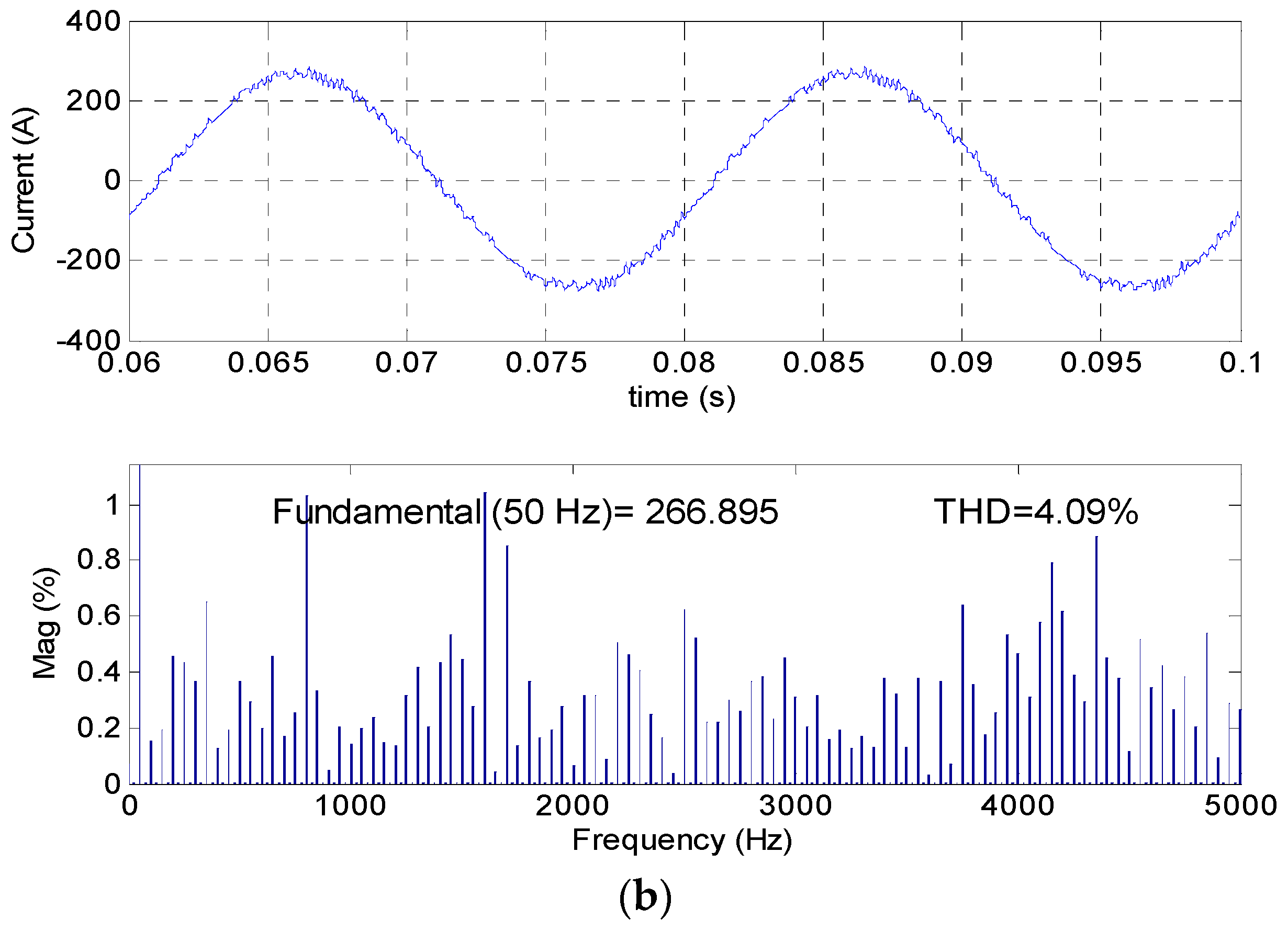
To obtain a better comparison in terms of line currents, the zoom-in waveforms and the harmonic spectrum are plotted out in Figure 8. It can be seen that the current when using the PDFC strategy is much more sinusoidal than that when using the conventional SDFC method. The total harmonic distortion (THD) of the line current for PDFC is 4.09%, much less than the 12.15% for SDFC. This is a significant improvement of the grid-connected DG system by using the inverter flux control approach.
5.2. Dynamic Performance
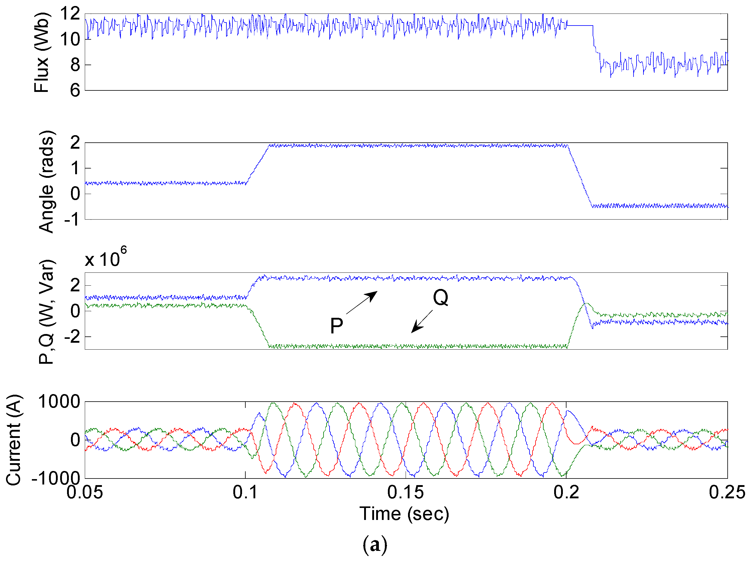
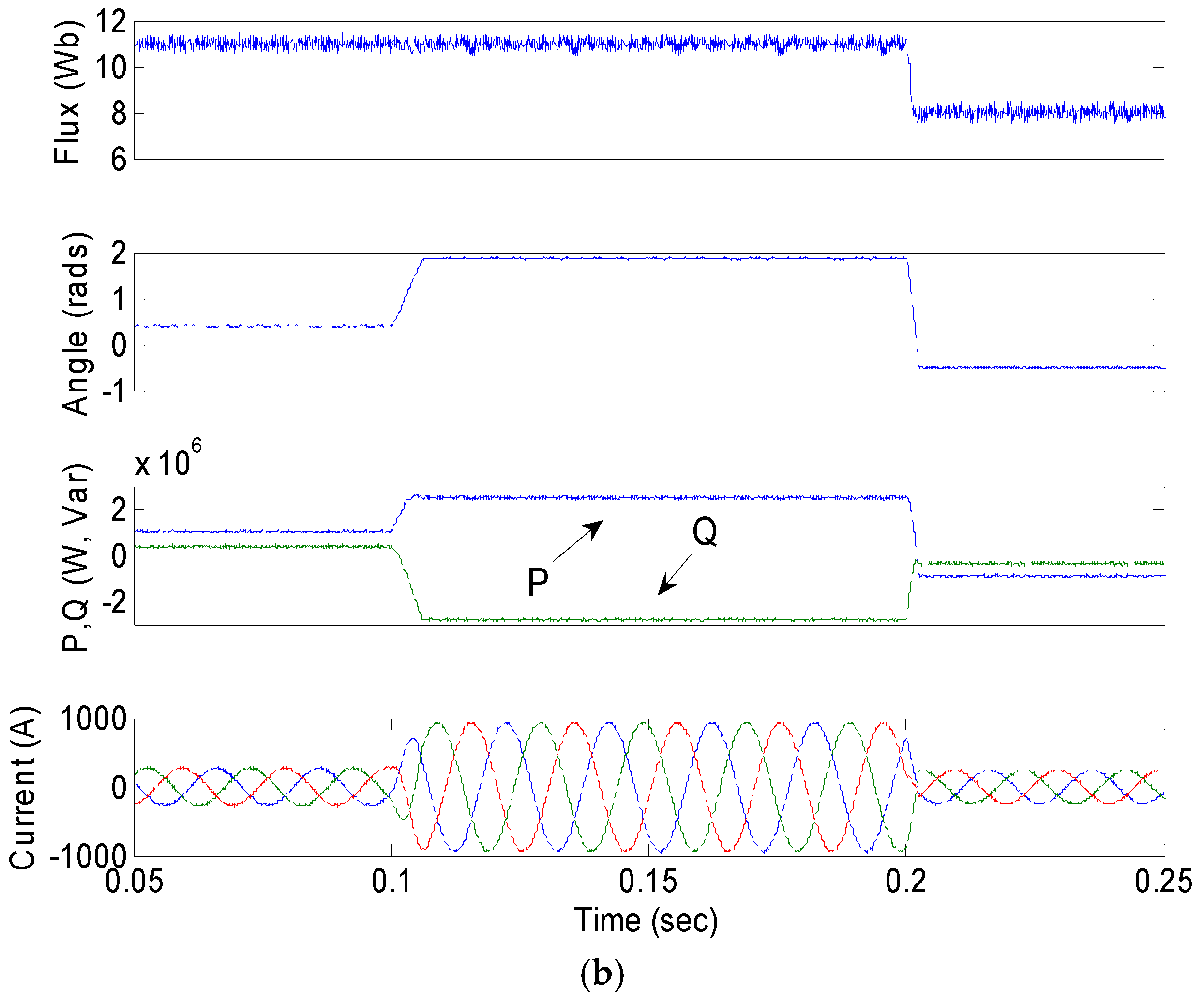
To further verify the reliability of the proposed inverter controller, the dynamic response is tested under the command of the stepped change of the flux magnitude and power angle. The flux amplitude reference steps down from 11 Wb to 8 Wb at a 0.2 s, while the power angle reference steps up from 0.4 rads to 1.9 rads at 0.1 s and steps down to −0.5 rads. It can be seen from Figure 9 that the flux magnitude and power angle can reach the new state in a safe manner without causing dangerous overshoot currents for both methods. However, the flux amplitude and power angle in PDFC can track the reference more quickly, especially during the reference stepping down. Besides, smaller active and reactive power ripples of PDFC can also be observed. It is worth mentioning that the active power becomes negative when the power angle (δp = δV − δE) is controlled to be less than zero. This indicates that the VSI system supplies the power from energy resources to the grid if the inverter flux vector lags behind the grid flux vector.
6. Conclusions
This paper has proposed the PDFC method for VSIs to reduce flux ripple as well as to improve the current quality. In the proposed PDFC strategy, the system model, together with all the possible inverter switching states, is used to predict the future flux behaviors. The switch state (or voltage vector) that can minimize the error between the references and the flux amplitude and power angle is then selected to control the inverter. On the basis of this operation scheme, the inverter flux can be controlled to have a specified magnitude and a specified position relative to the grid flux. The proposed PDFC method can reduce the inverter flux ripples as well as control the active and reactive powers with a fast transient response and less line current distortions compared with the conventional SDFC method.
Acknowledgments
This work is supported in part by The Hong Kong Polytechnic University under Grant 1-ZE7J.
Conflicts of Interest
The author declares no conflict of interest.
References
- Buja, G.S.; Kazmierkowski, M.P. Direct torque control of PWM inverter-fed ac motors—A survey. IEEE Trans. Ind. Electron. 2004, 51, 744–757. [Google Scholar] [CrossRef]
- Ma, T.; Cintuglu, M.H.; Mohammed, O.A. Control of hybrid ac/dc microgrid involving energy storage and pulsed loads. IEEE Trans. Ind. Appl. 2017, 53, 567–575. [Google Scholar] [CrossRef]
- Yu, Y.; Li, H.; Li, Z.; Zhao, Z. Modeling and analysis of resonance in LCL-type grid-connected inverters under different control schemes. Energies 2017, 10, 104. [Google Scholar] [CrossRef]
- Kazmierkowski, M.P.; Krishnan, R.; Blaabjerg, F. Control in Power Electronics; Academic Press: San Diego, CA, USA, 2002. [Google Scholar]
- Mohan, D.; Zhang, X.; Foo, G.H.B. Three-level inverter-fed direct torque control of IPMSM with torque and capacitor voltage ripple reduction. IEEE Trans. Energy Convers. 2016, 31, 1559–1569. [Google Scholar] [CrossRef]
- Hu, J.; Zhu, J.; Dorrell, D.G. A new control method of cascaded brushless doubly fed induction generators using direct power control. IEEE Trans. Energy Convers. 2014, 29, 771–779. [Google Scholar] [CrossRef]
- Scoltock, J.; Geyer, T.; Madawala, U.K. A model predictive direct current control strategy with predictive references for MV grid-connected converters with LCL-filters. IEEE Trans. Power Electron. 2015, 30, 5926–5937. [Google Scholar] [CrossRef]
- Chae, W.; Won, J.; Lee, H.; Kim, J.; Kim, J. Comparative analysis of voltage control in battery power converters for inverter-based AC microgrids. Energies 2016, 9, 596. [Google Scholar] [CrossRef]
- Chandorkar, M.C.; Divan, D.M.; Adapa, R. Control of parallel connected inverters in standalone ac supply systems. IEEE Trans. Ind. Appl. 1993, 29, 136–143. [Google Scholar] [CrossRef]
- Chandorkar, M.C. New techniques for inverter flux control. IEEE Trans. Ind. Appl. 2001, 37, 880–887. [Google Scholar] [CrossRef]
- Antoniewicz, P.; Kazmierkowski, M.P. Virtual-flux-based direct power control of AC/DC converters with online inductance estimation. IEEE Trans. Ind. Electron. 2008, 55, 4281–4390. [Google Scholar] [CrossRef]
- Hu, J.; Zhu, J.; Lei, G.; Platt, G.; Dorrell, D.G. Multi-objective model-predictive control for high power converters. IEEE Trans. Energy Convers. 2013, 28, 652–663. [Google Scholar]
- Perez, M.A.; Rodriguez, J.; Fuentes, E.J.; Kammerer, F. Predictive control of ac-ac modular converters. IEEE Trans. Ind. Electron. 2012, 59, 2832–2839. [Google Scholar] [CrossRef]
- D’Antona, G.; Faranda, R.; Hafezi, H.; Bugliesi, M. Experiment on bidirectional single phase converter applying model predictive current controller. Energies 2016, 9, 233. [Google Scholar] [CrossRef]
- Kouro, S.; Cortes, P.; Vargas, R.; Ammann, U.; Rodriguez, J. Model predictive control—A simple and powerful method to control power converters. Trans. Ind. Electron. 2009, 56, 1826–1838. [Google Scholar] [CrossRef]
- Hu, J.; Zhu, J.; Dorrell, D.G. In-depth study of direct power control strategies for power converters. IET Power Electron. 2014, 7, 1810–1820. [Google Scholar] [CrossRef]
- Mahmoudi, H.; Aleenejad, M.; Moamaei, P.; Ahmadi, R. Fuzzy adjustment of weighting factor in model predictive control of permanent magnet synchronous machines using current membership functions. In Proceedings of the IEEE Power and Energy Conference, Champaign, IL, USA, 19–20 September 2016. [Google Scholar]
- Muddineni, V.P.; Bonala, A.K.; Sandepudi, S.R. Enhanced weighting factor selection for predictive torque control of induction motor drive based on VIKOR method. IET Electr. Power Appl. 2016, 10, 877–888. [Google Scholar] [CrossRef]
Figure 1.
Equivalent circuit of the grid-connected voltage source inverter (VSI) system.

Figure 2.
Possible voltage vectors generated by the inverter.

Figure 3.
Illustration of inverter flux and grid flux in the α-β plane.

Figure 4.
Conventional direct flux control strategy of inverters.

Figure 5.
Proposed predictive direct flux control (PDFC) scheme.
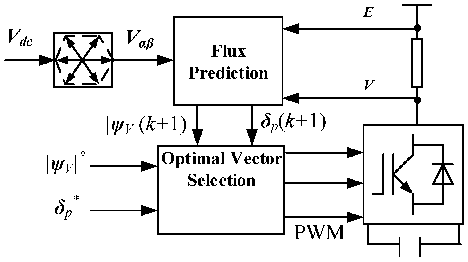
Figure 6.
Steady-state response. (a) Switching table–based direct flux control (SDFC); (b) Predictive direct flux control (PDFC).
Figure 6.
Steady-state response. (a) Switching table–based direct flux control (SDFC); (b) Predictive direct flux control (PDFC).

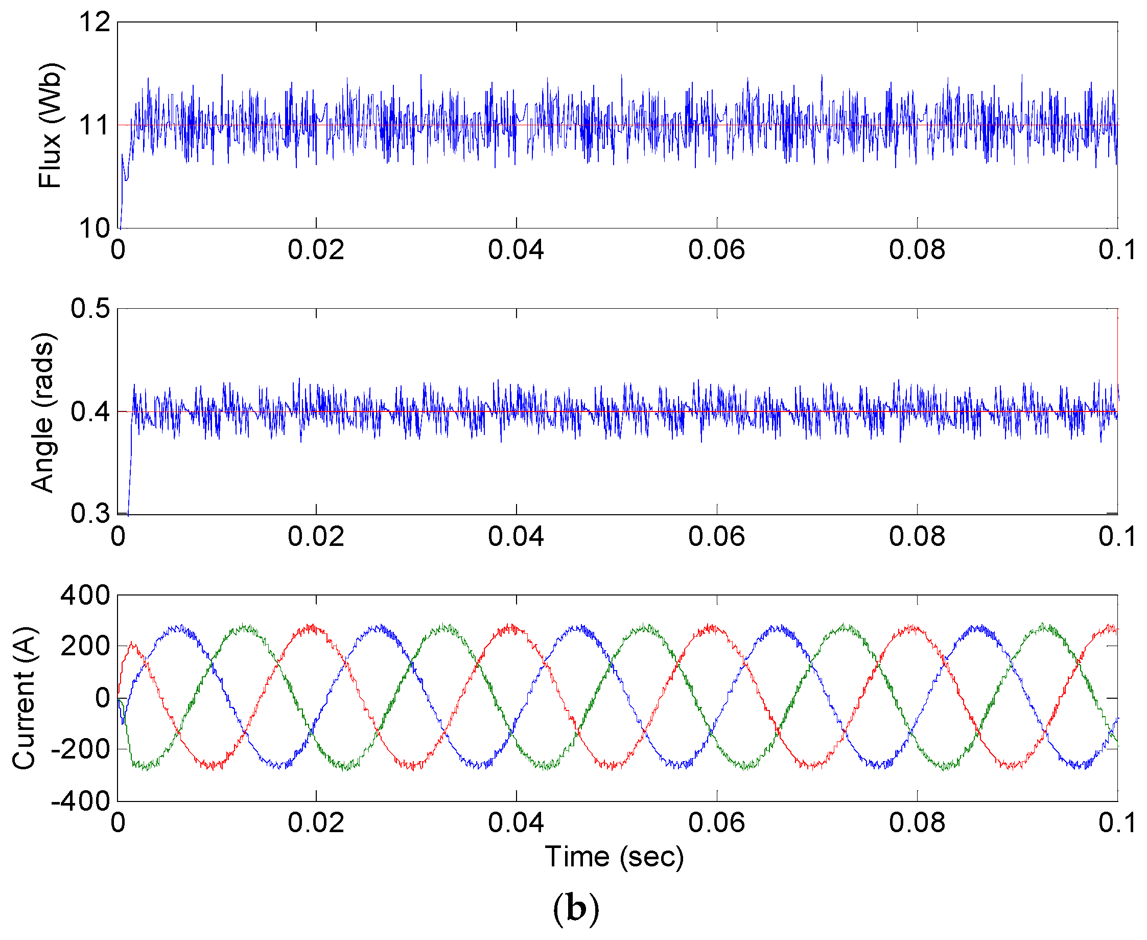
Figure 7.
The locus of inverter flux by using different control methods. (a) SDFC; (b) PDFC.

Figure 8.
FFT analysis of line currents. (a) SDFC; (b) PDFC.


Figure 9.
Dynamic response. (a) SDFC; (b) PDFC.


Table 1.
Switching table–based direct flux control (SDFC) switching table.
| Flux Regulation | Sector Number (Location of ΨV) | |||||
|---|---|---|---|---|---|---|
| S1 | S2 | S3 | S4 | S5 | S6 | |
| dF = 1, increase |ΨV| | V2 | V3 | V4 | V5 | V6 | V1 |
| dF = 0, decrease |ΨV| | V3 | V4 | V5 | V6 | V1 | V2 |
| dA = 0, null vector is applied to decrease δp | ||||||
Table 2.
System parameters.
| Quantity | Symbol | Value |
|---|---|---|
| Line Resistance | R | 0.51 Ω |
| Line inductance | L | 20 mH |
| Line-line grid voltage | E | 3.3 kV (rms) |
| System frequency | f | 50 Hz |
| DC-link voltage | Vdc | 10 kV |
| Sampling period | Ts | 100 μs |
© 2017 by the author. Licensee MDPI, Basel, Switzerland. This article is an open access article distributed under the terms and conditions of the Creative Commons Attribution (CC BY) license (http://creativecommons.org/licenses/by/4.0/).
Share and Cite
MDPI and ACS Style
Hu, J. Predictive Direct Flux Control—A New Control Method of Voltage Source Inverters in Distributed Generation Applications. Energies 2017, 10, 428. https://doi.org/10.3390/en10040428
AMA Style
Hu J. Predictive Direct Flux Control—A New Control Method of Voltage Source Inverters in Distributed Generation Applications. Energies. 2017; 10(4):428. https://doi.org/10.3390/en10040428
Chicago/Turabian StyleHu, Jiefeng. 2017. "Predictive Direct Flux Control—A New Control Method of Voltage Source Inverters in Distributed Generation Applications" Energies 10, no. 4: 428. https://doi.org/10.3390/en10040428
Note that from the first issue of 2016, this journal uses article numbers instead of page numbers. See further details here.