
Numerical Analysis of an Organic Rankine Cycle with Adjustable Working Fluid Composition, a Volumetric Expander and a Recuperator

School of Engineering, University of Glasgow, Glasgow G12 8QQ, UK
*
Author to whom correspondence should be addressed.
Energies 2017, 10(4), 440; https://doi.org/10.3390/en10040440
Submission received: 31 January 2017
/
Revised: 10 March 2017
/
Accepted: 22 March 2017
/
Published: 27 March 2017
(This article belongs to the Special Issue Recent Advances in Organic Rankine Cycle Technology for Stationary Applications)
Abstract
:Conventional Organic Rankine Cycles (ORCs) using ambient air as their coolant cannot fully utilize the greater temperature differential available to them during the colder months. However, changing the working fluid composition so its boiling temperature matches the ambient temperature as it changes has been shown to have potential to increase year-round electricity generation. Previous research has assumed that the cycle pressure ratio is able to vary without a major loss in the isentropic efficiency of the turbine. This paper investigates if small scale ORC systems that normally use positive-displacement expanders with fixed expansion ratios could also benefit from this new concept. A numerical model was firstly established, based on which a comprehensive analysis was then conducted. The results showed that it can be applied to systems with positive-displacement expanders and improve their year-round electricity generation. However, such an improvement is less than that of the systems using turbine expanders with variable expansion ratios. Furthermore, such an improvement relies on heat recovery via the recuperator. This is because expanders with a fixed expansion ratio have a relatively constant pressure ratio between their inlet and outlet. The increase of pressure ratio between the evaporator and condenser by tuning the condensing temperature to match colder ambient condition in winter cannot be utilised by such expanders. However, with the recuperator in place, the higher discharging temperature of the expander could increase the heat recovery and consequently reduce the heat input at the evaporator, increasing the thermal efficiency and the specific power. The higher the amount of heat energy transferred in the recuperator, the higher the efficiency improvement.
1. Introduction
Global energy use is predicted to continue to grow over the coming decades. Diminishing fossil fuel reserves and concerns about climate change mean that this extra energy demand will have to be supplied from non-conventional sources, many of which provide heat at temperatures too low to be exploited with traditional methods. Steam power plants become uneconomical for heat sources with temperatures below 400 °C due to declining efficiency combined with increasing component sizes due to low-pressure operation [1,2]. Several alternative methods exist for exploiting heat sources at such low temperatures, including the Stirling Cycle, Organic Rankine Cycle (ORC), and Kalina Cycle. However, Bianchi and De Pascale [3] have identified the Organic Rankine Cycle as the most promising technology for their utilisation. Typical heat sources for the Organic Rankine Cycle include solar, geothermal, biomass and industrial waste heat [4]. These heat sources have temperatures ranging from 80 °C for solar ponds, to over 500 °C for high-grade industrial waste heat [4], of which most exist at temperatures between 100 °C and 300 °C [5,6].
Organic Rankine Cycles replace water with an organic working fluid, which can exhibit superior thermal characteristics at low temperatures [7]. Most cycles use pure, single-component working fluids [8,9], however, there is also the potential to use a working fluid mixture. Organic Rankine Cycles are a relatively mature technology, with some market penetration, especially for geothermal applications. Their efficiency is often improved by the utilisation of a recuperative cycle [10,11], in which an internal heat exchanger is used to recover thermal energy from the expander exhaust that would otherwise be rejected in the condenser and use it to preheat the working fluid before it enters the evaporator. In this way, the heat that would otherwise be rejected from the cycle through the condenser is used to reduce the demand for input energy in the evaporator.
Drescher and Brüggemann [12] performed an in-depth analysis of working fluids for biomass ORCs, between temperatures of 90 °C and 350 °C, finding a maximum efficiency of 25% for a recuperative cycle operating towards the higher end of this range. Andreasen et al. [13] performed a working fluid screening for lower heat source temperatures of 90 °C and 120 °C, with a maximum efficiency of 10.3% for the higher temperature heat source. Bruno et al. [14] analysed solar powered ORCs for reverse osmosis desalination, and found that the efficiency of the cycle strongly depended on the selection of working fluid, and also the heat source temperature, varying from 7% to over 30% at the highest heat source temperatures.
Organic Rankine Cycles do suffer from several issues. Firstly, the constant temperature during phase change increases the temperature mismatch in the heat exchangers, increasing exergy destruction, and reducing the utilisation of the heat source for non-isothermal heat sources and sinks [15]. Yu et al. [16] identified a linear relationship between the integrated average temperature difference in the heat exchanger and the rate of exergy destruction. Secondly, the choice of pure working fluid is limited, meaning that not every application has an ideal working fluid. Organic Rankine Cycles are generally designed with a working fluid to match the temperatures of the heat source and heat sinks. Xu and Yu [17] showed that the efficiency of a subcritical ORC is related to the critical temperature of the working fluid. They found that the cycles tended to be less efficient when the difference between the heat source temperature and the critical temperature of the fluid becomes greater. Single-component working fluids have a particular critical temperature, and so if the critical temperature doesn’t match the operational conditions, a loss in efficiency will result. Thirdly, the small temperature differential provided by a low-enthalpy heat source means that the cycles are very sensitive to changing temperature of coolant, which can be proportionally significant compared to the cycle’s driving temperature differential. This has been identified as a problem hindering thermal cycles across the world [18]. It is of particular concern for cycles using air-cooled condensers, which are common for applications where portability or modularity is considered important, or where cooling water is too scarce or expensive. The heat sink for these cycles is the ambient air which, in continental climates, can vary in temperature by over 50 °C between summer and winter, and also a significant amount between day and night, as shown in previous research by the authors [19].
A cycle designed to operate in such conditions must ensure that liquid working fluid is fed to the pump at all times, as to allow vapour to be ingested into the pump compromises its efficiency and can even lead to damage due to cavitation. This requires a high condenser pressure, which means that when the ambient air is at a lower temperature, the cycle must either reduce the flow rate of coolant, or operate with significant subcooling at the pump outlet, which increases the heat energy required in the evaporator without any corresponding increase in expander work, reducing the cycle’s efficiency. This means that for much of the year, the cycle is operating at off-design conditions.
The authors have recently proposed that these issues can be solved by the concept of a dynamic ORC, capable of adjusting the composition of the working fluid during operation to match the changing ambient conditions [20]. When two working fluids are combined, they can generally form what is known as a zeotropic mixture [21]. This means that, instead of undergoing phase change at a constant temperature, like pure, single-component fluids, they instead exhibit a temperature change during phase change, known as “glide”. The lower temperature end of the phase change is known as the bubble point, and the higher temperature end is known as the dew point. The bubble and dew points of a zeotropic mixture lie between the boiling points of its two constituent parts. This means that with two components having different boiling points, a zeotropic mixture with a specific bubble or dew point temperature in between these two points can be formed by mixing them together. Given the right working fluid components, this can ensure that the pump in an Organic Rankine Cycle system is fed liquid for any ambient temperature between these two points. Several sources have concerned themselves with the efficiency of cycles using zeotropic mixtures as the working fluids, and found that they only cause a slight drop in cycle first law efficiency, while resulting in an increase in other metrics, such as heat source utilisation [22,23,24].
The proposed dynamic ORC system builds on this concept, by allowing the working fluid’s composition to be actively tuned during operation of the rig, using R245fa and R134a as the two components of the working fluid. These fluids are two commonly-selected ones for conventional Organic Rankine Cycles [25,26,27], are miscible with each other [28], and the difference between their boiling points is roughly equal to the annual variation in temperature in a continental climate, making them the most suitable for an initial analysis of this cycle. However, both of these fluids are HFCs (Hydrofluorocarbons), and this class of refrigerants has recently been subject to a phase-out decision over the coming decades due to their high Global Warming Potential. For a dynamic cycle, the key factor in the choice of fluids is an appropriate difference between their boiling points. Alternatives to HFCs do exist, and are presented below.
Alkanes are a promising class of working fluid, and in particular pentane and isopentane have been used in real-world cycles [2]. Alkanes tend to be relatively dry working fluids, meaning that they are particularly suitable to the presence of a recuperator. They are also flammable, which means that special care must be taken with their handling, Alkanes are a large class of refrigerants and this means that working fluid pairs for a great variety of ambient conditions can be selected.
HFOs (Hydrofluoro-olefins) are another fluid group under consideration in literature as a direct replacement for HFCs. R1233zd-E is the HFO replacement for R245fa [29], and R1234yf and R1234ze have been considered as replacements for R134a [27,30]. HFOs have very similar properties to HFCs, often being considered as “drop-in” replacements. R1233zd has been shown to give slightly higher thermal efficiencies than R245fa under the same operating conditions, whereas R1234yf showed slightly reduced power output due to lower density at the expander inlet. Overall they are likely to be no less suited to use in a dynamic ORC than the HFCs considered in this paper, but an investigation of alternative working fluids is an interesting avenue of further research.
The cycle is initially designed to operate on the hottest day of the year with the working fluid composed entirely of R245fa, the fluid component with the higher boiling point. As the temperature drops from summer to autumn, the temperature of the coolant available to the cycle also drops. This gives excess cooling capacity. The composition of the working fluid is then adjusted by removing fluid from the receiver and replacing it with pure R134a, shifting the overall composition towards R134a. This lowers the bubble point of the fluid, and allows better utilisation of the coolant. As the temperature drops further, the composition is shifted further towards R134a. The fluid mixture removed from the system is separated by distillation to produce pure R134a and R245fa, which can then be used in further composition tuning operations. In the spring, when temperatures begin to rise again, the available coolant is no longer cold enough to ensure the working fluid is liquid at the pump inlet. Now the composition of the working fluid is shifted back towards R245fa, raising the bubble point of the fluid and ensuring the liquid condition at the pump inlet.
The previous paper [19] considered a cycle using a turbine as the expander, and assumed that such a cycle can relatively simply adjust its evaporating pressure in operation by changing the shaft load on the turbine and increasing the pump power accordingly, with little change in the turbine’s isentropic efficiency. This allows the pressure ratio of the cycle to be changed in operation, increasing the evaporator pressure when the working fluid is mostly composed of R134a to minimise excess superheat. The results of this paper [19] showed a significant increase in the year-round electricity generation of a dynamic cycle compared to a conventional one. An economic analysis of the dynamic cycle was also carried out, using the Chemical Engineering Plant Cost Index (CEPCI). This revealed that the additional cost of a composition tuning system capable of distilling the system’s entire charge of working fluid in 12 h was roughly 0.4% of the total cost of the system, and that the greatest increase in the capital cost of a dynamic system would come from the need to have a supply of extra working fluid for tuning purposes, which would add a further 6% to the cost of the cycle. The increased cost of the system was offset by increased electricity generation. For any increase greater than 7% the payback period of the cycle was shortened and the 20-year return on investment increased.
However, turbines become uneconomical for smaller-scale applications below a few hundred kilowatts, and are outcompeted by positive displacement expansion devices, such as scroll, screw, and rotary vane expanders [30]. Quoilin et al. [31] have calculated the minimum economical operating power for a turbine in an ORC system to be roughly 40 kW for solar thermal applications, rising to over 100 kW for geothermal. This leaves a large amount of microgeneration applications for which turbines are unsuited as expanders.
Positive displacement devices generally have an inbuilt volume ratio, which is constrained by their geometry. The isentropic efficiency of these devices drop off sharply if a pressure ratio different to that defined by an adiabatic expansion process between these volumes is imposed [32,33,34]. This pressure ratio is hereafter referred to as the “designed pressure ratio”. The working fluid in the expander is enclosed in an expansion chamber. In each case, the enclosed volume of working fluid will reach the discharge stage at a pressure defined primarily by the geometry of the expander. If this pressure is not equal to the condenser pressure, the fluid will undergo an isochoric pressure drop (i.e., under-expansion) or increase (i.e., over expansion). In the case of under-expansion, when the in-built volume ratio of the expander could provide a pressure ratio less than the actual pressure ratio between the evaporator and condenser, this will result in unused potential of the working fluid. In the case of over-expansion, when the in-built volume ratio of the expander could provide a pressure ratio greater than the actual pressure ratio between the evaporator and condenser, work will have to be expended by the expander to repressurise the fluid to the condenser pressure. Therefore, the previous approach to the dynamic cycle using a turbine as the expansion device is not applicable to small-scale ORC systems.
As the considerations for designing ORC systems with positive displacement expanders are significantly different from those with turbines, this paper expands on the previous work by investigating whether the dynamic ORC concept can be applied to systems using a positive displacement expander which is constrained to a specific expansion ratio (ultimately pressure ratio). It analyses the system under a variety of ambient conditions, heat source temperatures and cycle configurations, both recuperative and non-recuperative to determine the feasibility of the development of dynamic Organic Rankine Cycle systems using positive displacement expanders having a fixed expansion ratio. It also adds an analysis of recuperative cycles applied to this dynamic concept, as well as an analysis of the specific power of the cycle and how this is affected by the changing working fluid composition in response to changing ambient temperature.
2. Numerical Modelling
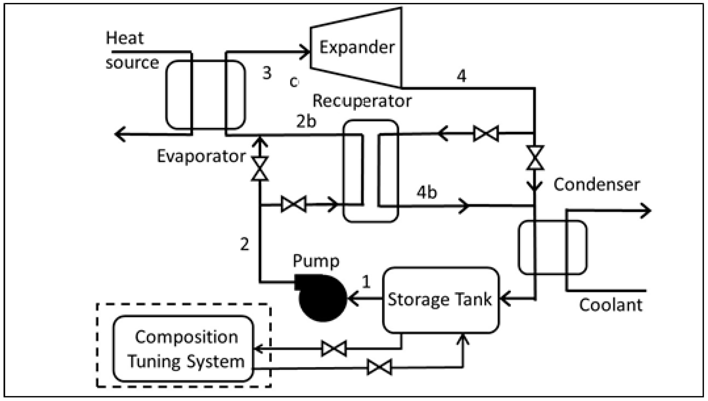
As shown in Figure 1, a dynamic Organic Rankine Cycle consists of the same major components as a standard Organic Rankine Cycle, namely the evaporator, expander, condenser, recuperator, and pump. In addition to these, the dynamic cycle has a composition tuning system attached to it. In order to simplify the analysis in this paper, the composition tuning system was considered to be a “black box”, capable of separating the working fluid into its two component parts, and reintroducing measured amounts of these pure components into circulation in the system. It was assumed to have no significant transient effects on the performance of the system as a whole apart from the change in working fluid composition. In practice such a system would most likely be a small distillation column, which is well-established technology. Previous research from the authors showed that the extra power required for a distillation system to keep up with changing ambient conditions is negligible compared to the overall power output of the cycle, as the average parasitic power required for separating and compressing the distillate would be 23 W for a 1 MW system [19].
There was assumed to be no pressure losses as the fluid passed through heat exchangers. This is a common assumption, but does not entirely reflect real world systems accurately. Real-world systems will experience pressure drops, especially in heat exchangers. The primary effect of this is that the pressure ratio at the expander inlet is reduced compared to the ideal case. A preliminary investigation assuming a 5% pressure drop in each heat exchanger, as was carried out in [34], indicating that in a recuperative cycle this would cause an 18% decrease in pressure ratio, and a 14% decrease in expander power, while the evaporator heat load remained relatively constant. For a non-recuperative cycle, the pressure ratio decreased by 14%, causing a 10% drop in expander power. These pressure losses must be carefully considered in the design of real-world systems. However, for comparison of the dynamic and non-dynamic ORCs, the pressure losses will not have a major effect on the differences caused by the working fluid composition.
Further assumptions were that there was no heat transfer to and from the system outside of heat exchangers (i.e., a perfectly insulated system), and no effects due to changes in velocity, elevation, or compressibility. The work required to pump heat transfer fluids through the heat exchangers was neglected in this research. Based on these assumptions, a standard steady-state numerical model was built using MATLAB R2016a (Mathworks, Natick, MA, USA) and REFPROP 9.1 (National Institute of Standards and Technology: Gaithersburg, MD, USA) [35]. REFPROP 9.1 was used to provide values for the thermophysical properties of the working fluid, and can be called via MATLAB function. Given a state defined by two fluid properties, this function can calculate most other important thermal and physical properties of a fluid at this state.
Figure 2 shows the numbering convention for the points of the cycle, which are the same as those shown in Figure 1. An external data file containing average monthly ambient temperature data for a variety of locations in different climate types was linked to the numerical model. The ambient temperature data from this data file could be used to determine the temperature of coolant available to the system over the course of the year, which was stored as an array in MATLAB. Beijing, China was chosen to use as a case study as it is an example of a continental climate with a high variation in temperature between winter and summer. The output power for the case study was selected as 10 kW. The pinch point temperature difference in the heat exchangers was taken to be 5 °C which is consistent with previous research [36,37], and an additional 2 °C of subcooling was added to the cycle at State 1 to ensure an adequate Net Positive Suction Head was provided to the pump. This allowed the condition of the working fluid at State 1 to be characterised using the equations and .
Knowing the temperature of the fluid and the required saturation temperature allows the condenser pressure to be determined for the hottest day of the year, which is also when the working fluid is composed entirely of the working fluid component with the higher boiling point, in this case study R245fa. REFPROP 9.1 can then be used to calculate the other fluid properties, such as specific entropy, and specific enthalpy. For a given pressure, REFPROP can also be used to calculate the bubble and dew points of a fluid as its composition changes, allowing a set of glide curves for the fluid pairing to be drawn up. Knowing the required condenser pressure and the shape of the bubble line of the glide curve, the required fluid composition to satisfy the liquid condition at the pump inlet can be calculated for any ambient temperature provided to the numerical model.
With the condenser pressure and fluid composition determined, the cycle can then be analysed using the real world climate data provided, according to well-established thermodynamic techniques [19,38]. The pinch point temperature in the evaporator is taken to be 5 °C as before, and a further 5 °C of superheat is added at the expander inlet to ensure a pure vapour with no droplets is fed into the expander, allowing the evaporator pressure to be calculated using the equations and .
This last was used to calculate the evaporator pressure on the hottest day of the year, and as the cycle in this case study uses a positive displacement expander, this evaporator pressure was held year-round. The isentropic efficiency of the pump and the expander were set to 90% and 70%, respectively. As the pressure ratio of the cycle was held constant over the year, the isentropic efficiencies of the pump and expander were also assumed to remain constant.
For the purposes of analysis, the pumping and expansion processes were initially assumed to be isentropic, allowing h2,isentropic and h4,isentropic to be determined using REFPROP. These values can then be used to find the actual values using an isentropic efficiency less than 100%, according the equations:
The isentropic efficiencies of the pump and expander were taken to be 90% and 70%, respectively. This is consistent with previous published literature. For this research, it was assumed that the expansion device used was designed with a volume ratio that would cause to operate at this efficiency at the imposed pressure ratio, i.e., a different expander would be required for a cycle operating at a different pressure ratio. The ratio of specific heats of the working fluids varies by less than 1% as the fluid composition is shifted from R245fa to R134a, so it was assumed that there would be no significant over- or under-expansion losses introduced due to changing fluid composition at a constant pressure and volume ratio.
Knowing the evaporator and condenser pressures, and the enthalpies at states 2 and 4, the temperatures and entropies at these states can now also be obtained using REFPROP.
The effect of a recuperator could also be investigated. The MATLAB program initially took the case of zero heat transfer from the hot to the cold side, giving a pinch point temperature difference of T4-T1. The program then gradually increased the amount of heat transferred while monitoring the temperature difference at 100 different points inside the heat exchanger, taking the minimum value as the new pinch point. When this pinch point reached 5 °C, the corresponding value of heat transfer could then be designated as Qrecuperator.
Once this has been done, all six points of the cycle have been characterized: pump outlet, recuperator outlet cold, evaporator outlet, expander outlet, recuperator outlet hot and condenser outlet. Equations (3)–(6) can then be used to calculate the efficiency of the cycle:
This allows the efficiency of the cycle to be calculated for any value of ambient temperature. Using real-world climate data as the values for ambient temperature allows, the performance of a dynamic ORC under various climate conditions to be analysed. The program analysed several key metrics. The first was the efficiency of the conventional ORC, ηcon, which was the efficiency of the cycle ηcycle on the hottest day of the year, when the working fluid had to be composed of 100% R245fa to ensure the liquid condition at the pump inlet. This is also the year-round efficiency of a cycle utilizing a fixed working fluid composition. The second was the efficiency of the dynamic ORC, ηdyn, for a given ambient temperature at a particular point in the year. Both of these were calculated according to Equation (6).
The third metric was the average annual efficiency of the dynamic ORC over the course of the year [19], . This is defined as:
where N is the number of operational days in the year [19].
The fourth was the annual improvement in energy provision ψ. This was given by the equation previously developed by the authors in [19]:
The pinch point in the heat exchangers could be analysed using an energy balance method. Using the assumption that the heat exchangers were perfectly thermally insulated from the environment, and that the temperature difference at the expander inlet was 10 °C, a T-Q diagram could be set up. As for the recuperator, the program took 100 points in the heat exchanger and calculated the temperature difference between the hot and cold streams. The temperature of the thermal fluid (assumed to be pressurised water in this case study) after transferring a certain amount of energy to the working fluid could be calculated from the equation:
where . is the mass flow rate of the hot water and cp its specific heat capacity. The higher the flow rate, the smaller the temperature change of the water as it exchanges energy with the working fluid. The mass flow rate of water is therefore increased from zero until the pinch point reaches the required 5 °C in both the evaporator and condenser. Once the flow rate is known, the final and average temperatures can be calculated using the lever rule, assuming that the specific heat capacity of the thermal fluid remains constant, giving a straight line on the pinch point diagram.
Knowing the mass flow rate of the hot water, the specific power output of the cycle can be calculated. The specific power is defined here as the power output from the expander per unit of mass flow of hot fluid in the evaporator, or mathematically as:
where W’ is the specific power. This allowed a further performance metric to be defined, similar to the increase in annual energy generation ψ. This was the increase in average annual specific power, given the symbol ϕ and defined as:
where . is the specific work of the dynamic cycle and where . is the specific work of the conventional, non-dynamic cycle The exergy at a given state can be determined using the equation:
As the values for specific enthalpy h and specific entropies are known for all states in the system, as is the temperature of the reference state T0, the exergy at any point in the system can be calculated. This can be used to calculate the exergy destruction rate in each component:
For the pump, the exergy destruction rate can be given by:
For the recuperator by:
For the evaporator by:
For the expander by:
For the condenser by:
The Overall Exergy Efficiency of the cycle is given by:
A qualitative analysis of the effect of working fluid composition on the heat transfer process was also carried out. The Nusselt number is the ratio of total to conductive heat transfer in a fluid, and is generally calculated for each case using empirical correlations to experimental data. Alimoradi and Veysi [38] give a rough correlation for the Nusselt number in a shell-and tube heat exchanger of:
where Re is the Reynolds Number and Pr is the Prandtl Number of the fluid:
where is fluid density, u is fluid velocity, D is the characteristic length, μ is the kinematic viscosity, cp is the specific heat capacity, and k is the thermal conductivity. D was set to 1 cm and u to 1.5 m/s, and all of the other information for the calculation could be obtained from REFPROP.
The cycle was analysed for several heat source temperatures, for recuperative and non-recuperative cases, and for five ambient climate conditions. For each case, the dynamic cycle was compared to the conventional, non-dynamic cycle, as well as comparing the effect of using a recuperative or non-recuperative dynamic cycle.
3. Results
The MATLAB routine based on the equations given in the previous section was used to analyse a case study for the dynamic Organic Rankine Cycle. Figure 3 shows the annual variation in temperature, and the change in working fluid composition needed to ensure the liquid condition at the pump inlet for various climate conditions. It can be seen that in the colder winter months, a greater proportion of R134a in the working fluid can be tolerated due to the lower ambient temperature. During the warmer summer months, more R245fa must be present to ensure the bubble point of the fluid is high enough to ensure this condition.
The conditions for Beijing were taken as a case study for more in-depth analysis, as it has the greatest variation between summer and winter temperatures among the locations considered. It was also used in the authors’ previous study [19], which enables comparison.
Figure 4 shows the variation in the efficiency of the cycle depending on the ambient temperature. The heat source temperature is set as 100 °C. The winter temperature is cold enough for the working fluid to be liquid at the pump inlet, even when it is 100% R134a. As the ambient temperature increases, the efficiency remains constant, until the point at which the ambient temperature becomes too high for a 100% R134a working fluid to be a liquid at the pump inlet. At this point, R245fa must be introduced. The cycle efficiency then drops off with increasing ambient temperature. The recuperative cycle in a relatively linear fashion, whereas the basic cycle shows a concave shape.
Figure 5 shows the variation of the enthalpy change in the expander, evaporator, condenser and recuperator as the ambient temperature changes. It can be seen that the amount of energy transferred in the evaporator and condenser increases relatively linearly for the evaporator as the ambient temperature decreases, and in a slightly convex shape for the condenser. This can explain the shape of the response curve for the non-recuperative cycle seen in Figure 4.
The response curve in Figure 5 has a steeper slope for the evaporator than for the expander towards the right hand side of the graph, i.e., for operation under higher temperature ambient conditions. This means that the evaporator enthalpy change is more sensitive to changing ambient temperature in this region. As the temperature drops, the evaporator enthalpy change will therefore increase more quickly than the expander enthalpy change. This means that the efficiency of the cycle is relatively insensitive to changing ambient temperature in the higher ambient temperature regions. Any increase in expander enthalpy change is cancelled out by a corresponding increase in evaporator enthalpy change. At lower temperatures, for example from 270 K to 280 K, the curve in Figure 5 for the expander is steeper than the curve for the evaporator. This means that the efficiency of the cycle is more sensitive to changing ambient temperature in this region, resulting in a steeper slope for this part of the response curve in Figure 4.
For the recuperative cycle, the response curve for efficiency in Figure 4 does not show the same convex shape. This can also be explained using the data presented in Figure 5. The curve in Figure 5 for the recuperator has a convex shape, with a steep section at high ambient temperatures, a peak at about 275 K, then a decrease to a steady value below about 265 K. The energy recovered in the recuperator is subtracted directly from the energy required in the evaporator, thereby increasing efficiency. The convex shape of the recuperator curve in Figure 5 works to cancel out the factors causing the concave shape of the efficiency curve for the non-recuperative cycle, as seen in Figure 4. This results in the relatively straight line seen for the efficiency plot for the recuperative cycle seen in Figure 4. This can be explained by a combination of the temperature glide caused by a zeotropic fluid, and the principle of operation of the recuperator.
Figure 6 demonstrates this by comparing T-s diagrams for the cycle operating under high temperature and low temperature ambient conditions. The thick green section of the T-s plot represents the heat transferred in the recuperator. It can be seen that in the low-temperature ambient conditions in the right hand plot, there is significant superheat at the expander outlet. This means that the working fluid exiting the expander is significantly warmer than the working fluid exiting the pump, giving a greater driving temperature differential for the recuperator to exploit. This tends to increase the amount of heat transferred in the recuperator under low temperature conditions, as seen in Figure 5.
Also to be noted is the fact that the left hand figure, representing higher temperature ambient conditions, also happens to be the T-s diagram for a zeotropic fluid, and therefore exhibits a temperature glide during phase change. This can be seen to cause an increase in the temperature of the expander outlet relative to the pump outlet due to this glide, which will also tend to increase the amount of heat transferred in the recuperator. This could explain the slight drop in the amount of heat transferred in the recuperator at higher proportions of R134a in the working fluid, because as the working fluid once again approaches a pure fluid composition, the glide decreases, and counteracts the increase in heat energy transferred in the recuperator due to increasing superheat to some degree. The response of the dynamic cycle with changing ambient temperature clearly shows that the cycle has improved performance over a conventional Organic Rankine Cycle when the temperature is lower.
It can be seen from Figure 7 that the dynamic cycle performs better than the conventional cycle for both the recuperative and non-recuperative cases, with the greatest improvement occurring during the colder winter months, as predicted by the response curves shown in Figure 4. As the conventional ORC efficiency is based on the highest annual temperature, the lowest point of the monthly average for the dynamic cycle is still higher than this, as even during the hottest months, the temperature is generally lower than the maximum most of the time. The non-recuperative cycle increases in efficiency extremely slowly in response to decreasing temperature at the higher end of the temperature range, so the non-recuperative dynamic cycle only begins to significantly outperform the conventional cycle at the beginning and end of the year when the temperature is a great deal colder than the maximum. The efficiency of the recuperative dynamic cycle increases far more sharply with increasing temperature, and so the improvement can be seen even during the summer months, when the temperature is still close to the maximum used in the design of the conventional cycle.
The value of ψ changes depending on the annual variation in temperature, as shown in Figure 8. The MATLAB routine was run using climate data from several locations worldwide, for heat source temperatures of 100 °C and 150 °C. A steady increase in ψ can be seen as the amplitude of the temperature variations increases. This is to be expected, as the greater the temperature variation, the greater the difference between the hot and cold reservoirs, and therefore the greater the Carnot efficiency. The plot deviates slightly from the linear increase in Carnot efficiency, however, due to several factors, most notably the composition of the working fluid. When the temperature variation is small, only a small amount of R134a is needed to keep up with the changing heat sink temperature. When the temperature variation is much larger, the working fluid can be 100% R134a, and still have excess cooling capacity it is not utilising. Some small deviations from the theoretical smooth increase can be seen. For example, Phoenix has a higher average temperature than any of the other locations, and therefore a reduced conventional cycle efficiency. This means that the dynamic cycle is slightly more effective here than the idealised case would predict.
The trend for the non-recuperative cycles is of a slightly different shape, rising slowly at first, then increasing in slope. This is because, as shown in Figure 4, the efficiency of non-recuperative cycles only increase very slowly when the ambient temperature decreases from the annual maximum. At lower annual temperature variations, the heat sink temperature never becomes cold enough to cause the non-recuperative cycle to enter the region of its response curve where a sharp increase in efficiency can be seen.
The variation in ψ with changing heat source temperature was also investigated, and the results for the case study of Beijing’s climate conditions plotted in Figure 9. It can be seen that for both the recuperative and non-recuperative dynamic cycles, the improvement in annual energy provision ψ increases gradually until a temperature of 150 °C, whereat it peaks, and then begins to drop away. This is in contrast to the results previously obtained by the authors for a similar dynamic ORC concept using a turbine as the expander [19], in which the value of ψ smoothly decreased with increasing heat source temperature as the resulting increased Carnot efficiency of the conventional cycle made the gains caused by the dynamic cycle proportionally smaller.
It is significant that the peak in the plot of Figure 9 occurs at roughly the critical point of R245fa, at a temperature of 154 °C. As stated in the previous section, the MATLAB routine ensured that the cycle was subcritical, by selecting the evaporator pressure either to produce zero superheat at the expander inlet when the working fluid was 100% R245fa, or to 5 K below the critical temperature of the fluid, whichever was the lower.
Figure 10 shows the variation in the evaporator and condenser pressures as the heat source temperature is varied. In the lower range, increasing the heat source temperature allows the evaporator pressure to be increased, increasing the efficiency of the cycle. This trend continues until the critical point of R245fa is reached, at which point the pressure ratio cannot be increased any further without the cycle becoming supercritical. After this point, the cycle then shows the same trend as the previous cycle considered by the authors, with the increase in annual energy provision dropping off as the gains caused by the dynamic cycle become less proportionally significant.
The previous analysis has been a first-law treatment of the dynamic ORC. However, First Law Efficiency is only one metric by which a cycle can be analysed. For waste heat sources, for example, the specific power is a better metric by which to judge the cycle.
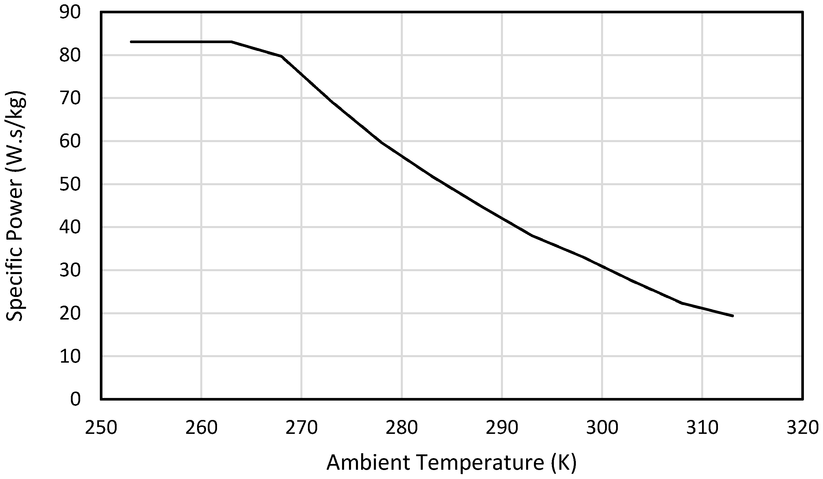
Figure 11 shows the variation in the specific power of the cycle as the ambient temperature changes. Two things are immediately apparent from the graph. Firstly, the specific power increases with decreasing ambient temperature. Secondly, the curves for the recuperative and non-recuperative cycles are identical.
The first point can be explained by examining the pinch point diagrams for the evaporator of the ORC. Figure 12 shows the evaporator pinch point diagrams for a high ambient temperature case, i.e., with the fluid composed of mostly R245fa, and a low ambient temperature case, i.e., with the fluid composed mostly of R134a. The lower boiling point of the R134a has resulted in a far greater degree of superheat at the expander inlet, allowing a much steeper line for the evaporator. The steeper line means a lower necessary mass flow rate of thermal fluid. The ORC has its output fixed at 10 kW, so the reduced mass flow rate observed in Figure 12 means that the specific power increases for the lower heat sink temperatures represented by the leftmost pinch point diagram.
The second point, the fact that the recuperative and non-recuperative curves are identical, can be explained by the fact that the pinch point in both cases is at the bubble point of the working fluid, and that the recuperator does not cause a phase change in the evaporator. Even though the energy transferred in the evaporator will be less in the recuperative case, meaning the first law efficiency increases, this does not necessarily translate into an increase in specific power, as the expander work is still held constant, and the thermal fluid line must still satisfy the pinch point condition. This means that unless the pinch point position changes, there can be no change in the flow rate on the hot side of the evaporator, and the specific power will not change. In no cases analysed was there a phase change in the recuperator, meaning that there was no difference between the recuperative and non-recuperative plots.
Figure 13 shows the variation in the increase in annual heat source utilization ϕ as the heat source temperature changes. It can be seen that the value initially drops off slowly as the heat source temperature is increased, due primarily to the increase in the minimum value of the specific power. As the heat source temperature approaches the critical temperature, the value of ϕ drops off more sharply. Figure 14 shows how the specific power of the non-dynamic cycle varies with heat source temperature for Beijing’s ambient conditions. It can be seen that the specific power of the non-dynamic cycle begins to increase at amount this point as well, due to the fact that after the critical temperature of R245fa at 154 °C there will be a superheat at the expander inlet for the non-dynamic cycle, allowing an increased slope on the T-Q diagram for the thermal fluid and reducing its required flow rate.
A brief caveat with regard to the analysis of specific power: Optimising the specific power output is a complex task. Reducing the evaporator pressure will increase expander inlet superheat, and tend to increase specific power, while reducing first law efficiency of the cycle. Reduced first law efficiency tends to increase the installed cost per kW of the cycle. The optimum point will depend on the exact application of the cycle and the details of the heat source. Such a specific analysis is outside the scope of the general treatment applied in this paper, but the analysis presented serves to show the general trend.
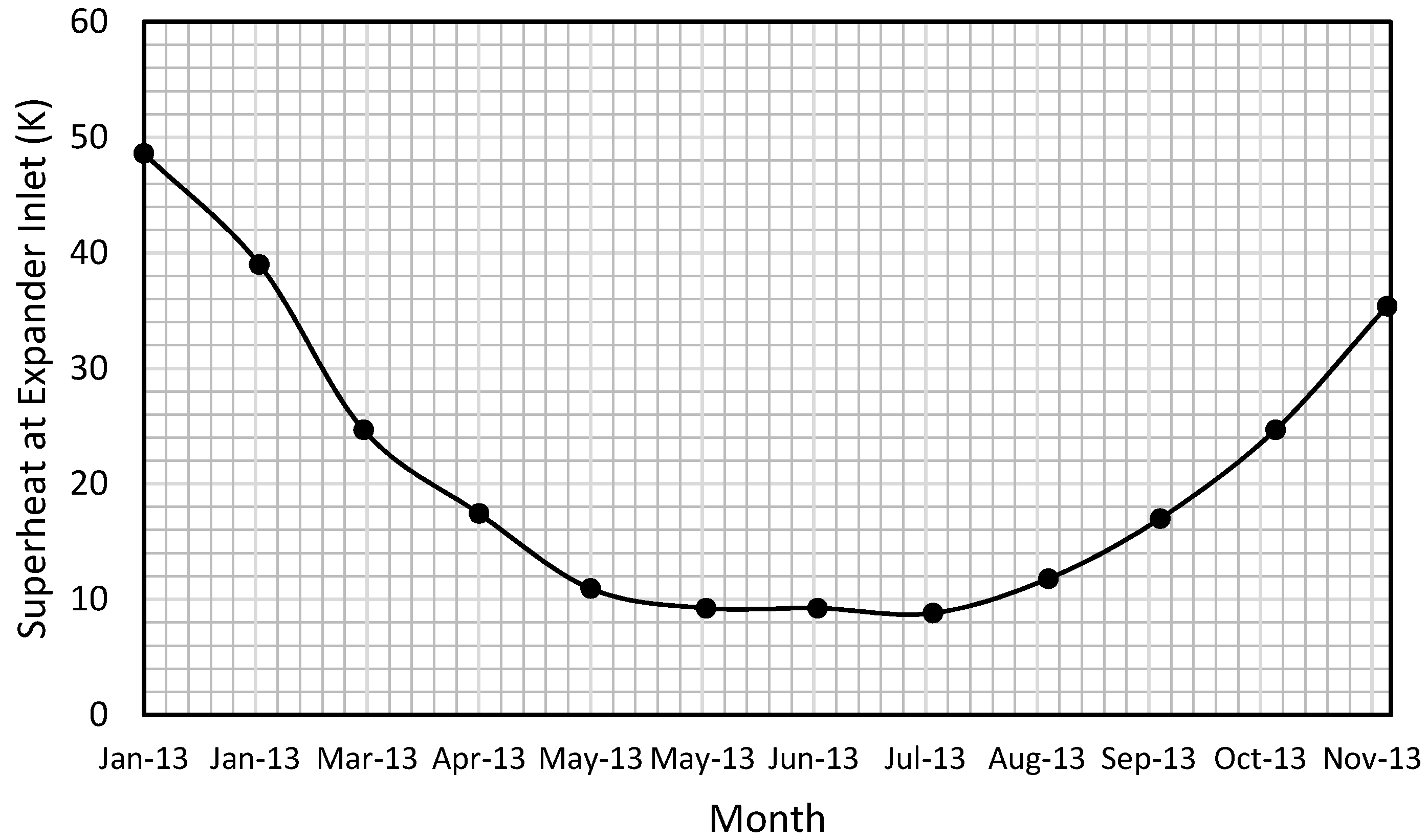
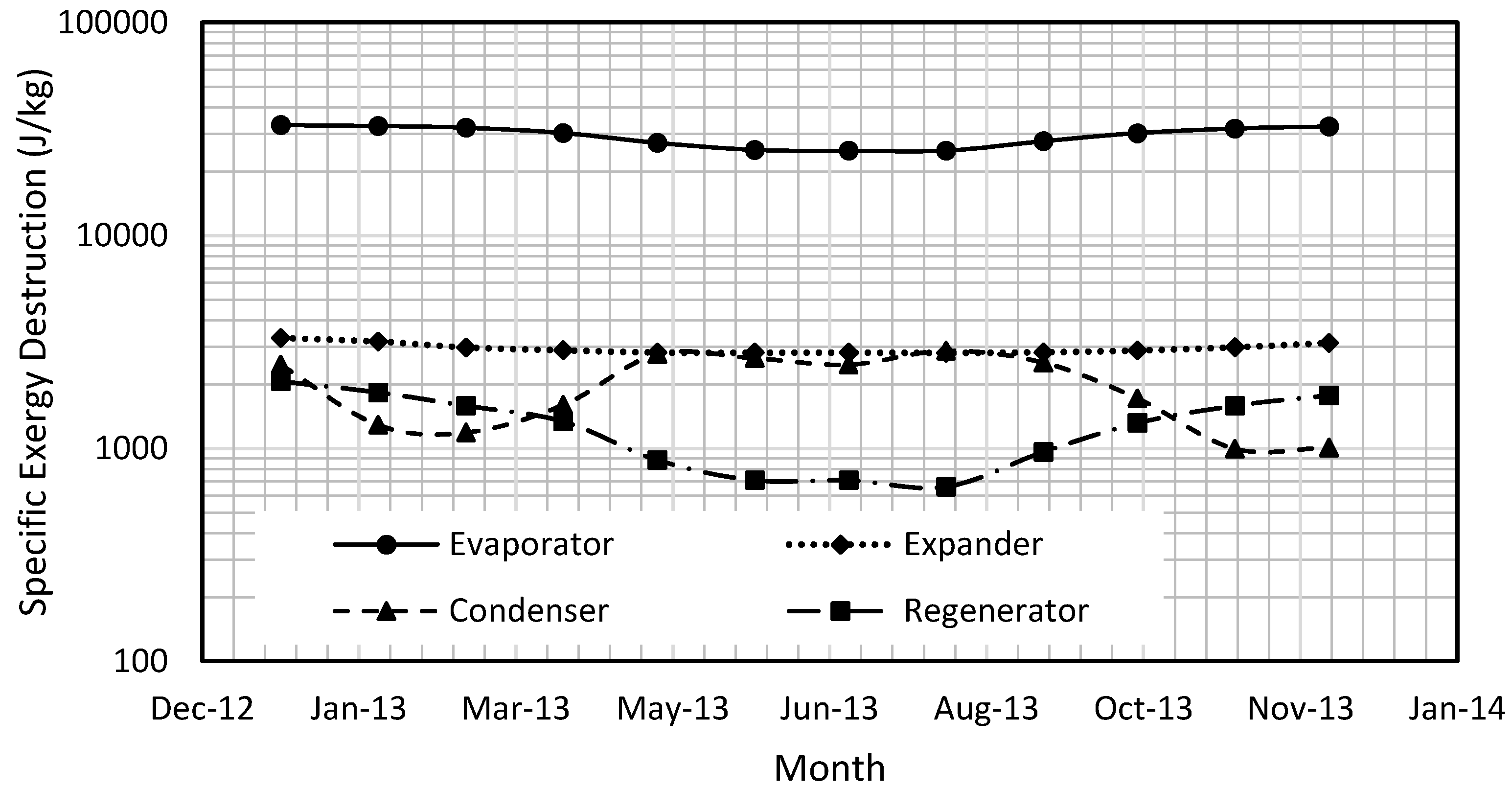
Figure 15 shows the variation in superheat over the course of the year. Figure 16 and Figure 17 show the exergy destruction in each component over the course of the year. Although some irreversibility occurred in the pump, resulting in exergy destruction, its effect was negligible in comparison to other components, and therefore has been left out of the following plots in the interest of clarity. It can be seen that with a recuperator present, the evaporator is by far the greatest contributor to exergy destruction. This exergy destruction is greatest during the winter months. This seems primarily to be caused by the greater degree of superheat introduced at the expander inlet by the shifting of the working fluid composition to one rich in R134a, which reduces its dew point.
The recuperator shows the lowest exergy destruction rate, indicating the highest recuperator efficiency, during the winter months, as was noted in the previous section. Figure 17 shows the similar results for the case of a non-recuperative cycle. The specific exergy destruction in the evaporator is higher in this case, reaching 37 kJ/kg, as opposed to 33 kJ/kg in the recuperative cycle. The exergy destruction in the condenser is also noticeably higher, reaching almost 14 kJ/kg during the winter months, which are when the recuperator is at its most effective.
The exergy efficiency of the cycle over the course of the year was also analysed. Figure 18 shows this variation for a heat source temperature of 75 °C. It can be seen that the exergy efficiency is higher year-round for the recuperative cycle, and that the recuperative and basic cycles diverge in the winter months as the recuperator takes up the excess heat at the expander inlet. All cycles show high second law efficiency in the summer months, which drops off slightly as the ambient temperature drops, the fluid composition changes, and the temperature mismatch in the evaporator increases.
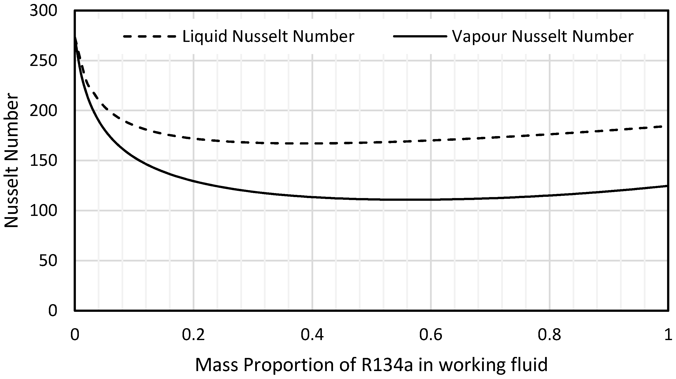
An analysis of how the heat transfer coefficients in the heat exchangers varied depending on working fluid composition was also carried out. Figure 19 shows how the Nusselt numbers for liquid and vapour varied depending on the working fluid composition.
It can be seen in Figure 19 that the Nusselt number is around 270 for the pure R245fa, drops to 110 for the vapour Nusselt number and 165 for the liquid Nusselt number. Even for a situation with minimal superheating of the working fluid, this implies that an oversized heat exchanger will be needed for the dynamic cycle compared to a non-dynamic cycle using R245fa as the working fluid. This will add to the capital cost of the dynamic cycle compared to a non-dynamic equivalent.
4. Conclusions
This paper investigates if the recently developed dynamic ORC cycle can be applied to small-scale systems based on positive-displacement expanders with fixed expansion ratios. The results show that the dynamic ORC is capable of increasing the system’s annual average efficiency for a given heat source. However, such an improvement is much less than that of the large scale system using turbine expanders with variable expansion ratios. Furthermore, such benefit strongly depends on heat recovery via the recuperator. The higher the heat recuperation, the higher the efficiency improvement. This is because an expander with a fixed expansion ratio approximately has a constant pressure ratio between its inlet and outlet. The increase of pressure ratio between the evaporator and condenser by tuning the condensing temperature to match colder ambient condition in winter cannot be utilized by such expanders. However, with the recuperator in place, the higher discharging temperature of the expander could increase the heat recovery and consequently reduce the heat input at the evaporator, ultimately increasing the thermal efficiency.
The dynamic cycle also showed an improvement in specific power, implying better heat source utilization. This was caused by increasing expander inlet superheat as the working fluid composition changed, allowing for the same amount of electricity to be generated from a smaller flow rate of thermal fluid.
An exergy analysis has also been conducted, and it was found that the exergy destruction in the cycle was dominated by the evaporator. The exergy efficiency was improved by the dynamic cycle, particularly in the winter months, as the recuperator and increased superheat caused by the change in working fluid composition made better use of the increased available driving temperature differential, compared to the conventional, non-dynamic cycle.
Acknowledgments
This research is funded by Royal Society (RG130051) and EPSRC (EP/N005228/1 and EP/N020472/1) in the United Kingdom, and a joint Programme “Royal Society–National Natural Science Foundation of China (Ref: IE150866)”.
Author Contributions
Zhibin Yu developed the initial concept. Peter Collings and Zhibin Yu performed the literature review and collaborated on the introduction. Peter Collings produced the mathematical model and MATLAB program. Peter Collings and Zhibin Yu analysed the results and interpreted the data. Peter Collings and Zhibin Yu wrote the paper.
Conflicts of Interest
The authors declare no conflict of interest.
References
- Hung, T.C.; Shai, T.Y.; Wang, S.K. A Review of Organic Rankine Cycles (ORCs) for the Recovery of Low Grade Waste Heat. Energy 1997, 22, 661–667. [Google Scholar] [CrossRef]
- Siddiqi, M.; Atakan, B. Alkanes as fluids in Rankine cycles in comparison to water, benzene and toluene. Energy 2012, 45, 256–263. [Google Scholar] [CrossRef]
- Bianchi, M.; Pascale, A. Bottoming Cycles for Electric Energy Generation: Parametric Investigation of Available and Innovative Solutions for the Exploitation of Low and Medium Temperature Heat Sources. Appl. Energy 2011, 88, 1500–1509. [Google Scholar] [CrossRef]
- Zhai, H.; An, Q.; Shi, L.; Lemort, V.; Quoilin, S. Categorisation and Analysis of Heat Sources for Organic Rankine Cycle Systems. Renew. Sustain. Energy Rev. 2015, 64, 790–805. [Google Scholar] [CrossRef]
- Barbier, E. Geothermal Energy Technology and Current Status: An Overview. Renew. Sustain. Energy Rev. 2002, 6, 3–65. [Google Scholar] [CrossRef]
- Freeman, J.; Hellgardt, K.; Markides, C. Working Fluid Selection and Electrical Performance optimisation of a Domestic Solar-ORC Combined Heat and Power System for Year-Round Operation in the UK. Appl. Energy 2016, 186, 291–303. [Google Scholar] [CrossRef]
- Tchanche, B.; Lambrinos, G.; Frangoudakis, A.; Papadakis, G. Low grade heat conversion into power using organic Rankine cycles—A review of various applications. Renew. Sustain. Energy Rev. 2011, 15, 3963–3979. [Google Scholar] [CrossRef]
- Wang, E.; Zhang, H.; Fan, B.; Ouyang, M.; Zhao, Y.; Mu, Q. Study of Working Fluid Selection of Organic Rankine Cycle (ORC) for Engine Waste Heat Recovery. Energy 2011, 36, 3406–3418. [Google Scholar] [CrossRef]
- Zhang, H.G.; Wang, E.H.; Fan, B.Y. A Performance Analysis of a Novel System of a Dual Loop Bottoming Organic Rankine Cycle (ORC) with a Light-Duty Diesel Engine. Appl. Energy 2013, 102, 1504–1513. [Google Scholar] [CrossRef]
- Ziviani, D.; Gusev, S.; Lecompte, S.; Groll, E.E.; Braun, J.E.; Horton, W.T.; Broek, M.; Paepe, M. Characterising the Performance of a Single-Screw Expander in a Small-Scale Organic Rankine Cycle for Waste Heat Recovery. Appl. Energy 2016, 181, 155–170. [Google Scholar] [CrossRef]
- Li, G. Organic Rankine Cycle Performance Evaluation and Thermoeconomic Assessment wth Various Applications part II. Renew. Sustain. Energy Rev. 2016, 64, 490–505. [Google Scholar] [CrossRef]
- Drescher, U.; Brüggemann, D. Fluid selection for the Organic Rankine Cycle (ORC) in biomass power and heat plants. Appl. Therm. Eng. 2007, 27, 223–228. [Google Scholar] [CrossRef]
- Andreasen, J.G.; Larsen, U.; Knudsen, T.; Pierobon, L.; Haglind, F. Selection and Optimisaion of Pure and Mixed Working Fluids for Low Grade Heat Utilisation Using Organic Rankine Cycle. Energy 2014, 73, 204–213. [Google Scholar] [CrossRef]
- Bruno, J.; Lopez-Villada, J.; Letelier, E.; Romera, S.; Coronas, A. Modelling and optimisation of solar organic rankine cycle engines for reverse osmosis desalination. Appl. Therm. Eng. 2008, 28, 2212–2226. [Google Scholar] [CrossRef]
- UNEP Ozone Secretariat. 1998 Report of the Refrigeration, Air Conditioners and Heat Pumps Technical Options Committee; UNEP: Geneva, Switzerland, 1998. [Google Scholar]
- Yu, C.; Xu, J.; Sun, Y. Transcritical Pressure Organic Rankine Cycle (ORC) Analysis based on the Integrated-Average Temperature Difference in Evaporators. Appl. Therm. Eng. 2015, 88, 2–13. [Google Scholar] [CrossRef]
- Xu, J.; Yu, C. Critical Temperature Criterion for Selection of Working Fluids for Subcritical Pressure Organic Rankine Cycles. Energy 2014, 74, 719–733. [Google Scholar] [CrossRef]
- Harinck, J.; Calderazzi, L.; Colonna, P.; Polderman, H. ORC Deployment Opportunities in Gas Plants. In Proceedings of the 3rd International Seminar on ORC Power Systems, Brussels, Belgium, 12–14 October 2015. [Google Scholar]
- Collings, P.; Yu, Z.; Wang, E. A Dynamic Organic Rankine Cycle using a Zeotropic Mixture as the Working Fluid with Composition Tuning to Match Changing Ambient Conditions. Appl. Energy 2016, 171, 581–591. [Google Scholar] [CrossRef]
- Collings, P.; Yu, Z. Modelling and Analysis of a Small-Scale Organic Rankine Cycle System with a Scroll Expander. In Proceedings of the World Congress on Engineering, London, UK, 2–4 July 2014. [Google Scholar]
- Chys, M.; Broek, M.; Vanslambrouck, B.; Paepe, M. Potential of Zeotropic Mixtures as Working Fluids in Organic Rankine Cycles. Energy 2012, 44, 623–632. [Google Scholar] [CrossRef]
- Angelino, G.; Paliano, P. Multicomponent Working Fluids for Organic Rankine Cycles (ORCs). Energy 1998, 23, 449–463. [Google Scholar] [CrossRef]
- Wang, X.D.; Zhao, L. Analysis of Zeotropic Mixtures Used in Low-Temperature Solar Rankine Cycles for Power Generation. Sol. Energy 2009, 83, 605–613. [Google Scholar] [CrossRef]
- Li, W.; Feng, X.; Yu, L.J.; Xu, J. Effects of Evaporating Temperature and Internal Heat Exchanger on Organic Rankine Cycle. Appl. Therm. Eng. 2011, 32, 4014–4023. [Google Scholar] [CrossRef]
- Mohammad, U.; Imran, M.; Lee, D.; Park, B. Design andd Experimental Investigation of a 1 kW Organic Rankine Cycle System Using R245fa as Working Fluid for Low-Grade Heat Recovery From Steam. Energy Convers. Manag. 2015, 103, 1089–1100. [Google Scholar] [CrossRef]
- Heberle, F.; Schifflechner, C.; Bruggemann, D. Life Cycle Assessment of Organic Rankine Cycles for Geothermal Power Generation Considering Low-GWP Working Fluids. Geothermics 2016, 64, 392–400. [Google Scholar] [CrossRef]
- Invernizzi, C.M.; Iora, P.; Preissinger, M.; Manzolini, G. HFOs as Substitute for R134a in ORC Power Plants: A Thermodynamic Assessment and Thermal Stability Analysis. Appl. Therm. Eng. 2016, 103, 790–797. [Google Scholar] [CrossRef]
- Abadi, G.; Yun, E.; Kim, K. Experimental Study of a 1kW Organic Rankine Cycle with a Zeotropic Mixture of R245fa/R134a. Energy 2015, 93, 2363–2373. [Google Scholar] [CrossRef]
- Eyerer, S.; Wieland, C.; Vandersickel, A.; Spliethoff, H. Experimental Study of an ORC (Organic Rankine Cycle) and analysis of R1233zd-E as a drop-in replacement for R245fa for low temperature heat utilization. Energy 2016, 103, 660–671. [Google Scholar] [CrossRef]
- Quoilin, S.; Declaye, S.; Lemort, V. Expansion Machine and Fluid Selection for the Organic Rankine Cycle. In Proceedings of the 7th International Conference on Heat Transfer, Fluid Mechanics and Thermodynamics, Antalya, Turkey, 19–21 July 2010. [Google Scholar]
- Quoilin, S.; Broek, M.; Declaye, S.; Dewallef, P.; Lemort, V. Techno-economic survey of Organic Rankine Cycle (ORC). Renew. Sustain. Energy Rev. 2013, 22, 168–186. [Google Scholar] [CrossRef]
- Quoilin, S.; Lemort, V.; Lebrun, J. Experimental study and modeling of an Organic Rankine Cycle using scroll expander. Appl. Energy 2010, 87, 1260–1268. [Google Scholar] [CrossRef]
- Bao, J.; Zhao, L. A review of working fluid and expander selections for Organic Rankine Cycle. Renew. Sustain. Energy Rev. 2013, 24, 325–342. [Google Scholar] [CrossRef]
- Read, M.; Smith, I.; Stosic, N.; Kovacevic, A. Comparison of Organic Rankine Cycle systems under Varying Conditions Using Turbine and Twin-Screw Expanders. Energies 2016, 9, 614. [Google Scholar] [CrossRef]
- Lemmon, E.W.; Huber, M.L.; McLinden, M.O. NIST Standard Reference Database 23: Reference Fluid Thermodynamic and Transport Properties-REFPROP; version 9.1; National Institute of Standards and Technology, Standard Reference Data Program: Gaithersburg, MD, USA, 2013.
- Clemente, S.; Micheli, D.; Reini, M.; Taccani, R. Simulation model of an Experimental Small-Scale ORC Cogenerator. In Proceedings of the First International Seminar on ORC Power Systems, Delft, The Netherlands, 22–23 September 2011. [Google Scholar]
- Liu, Q.; Duan, Y.; Yang, Z. Effect of condensation temperature glide on the performance of organic Rankine cycles with zeotropic mixture working fluids. Appl. Energy 2014, 115, 394–404. [Google Scholar] [CrossRef]
- Alimoradi, A.; Veysi, F. Prediction of Heat Transfer Coefficients of Shell and Coiled Tube Heat Exchangers using Numerical Method and Experimental Validation. Int. J. Therm. Sci. 2016, 107, 196–208. [Google Scholar] [CrossRef]
Figure 1.
Schematic Diagram of Dynamic Organic Rankine Cycle considered in this paper.

Figure 2.
T-s diagram of a zeotropic ORC, with the recuperative portion of the cycle marked in a thicker green line.
Figure 2.
T-s diagram of a zeotropic ORC, with the recuperative portion of the cycle marked in a thicker green line.
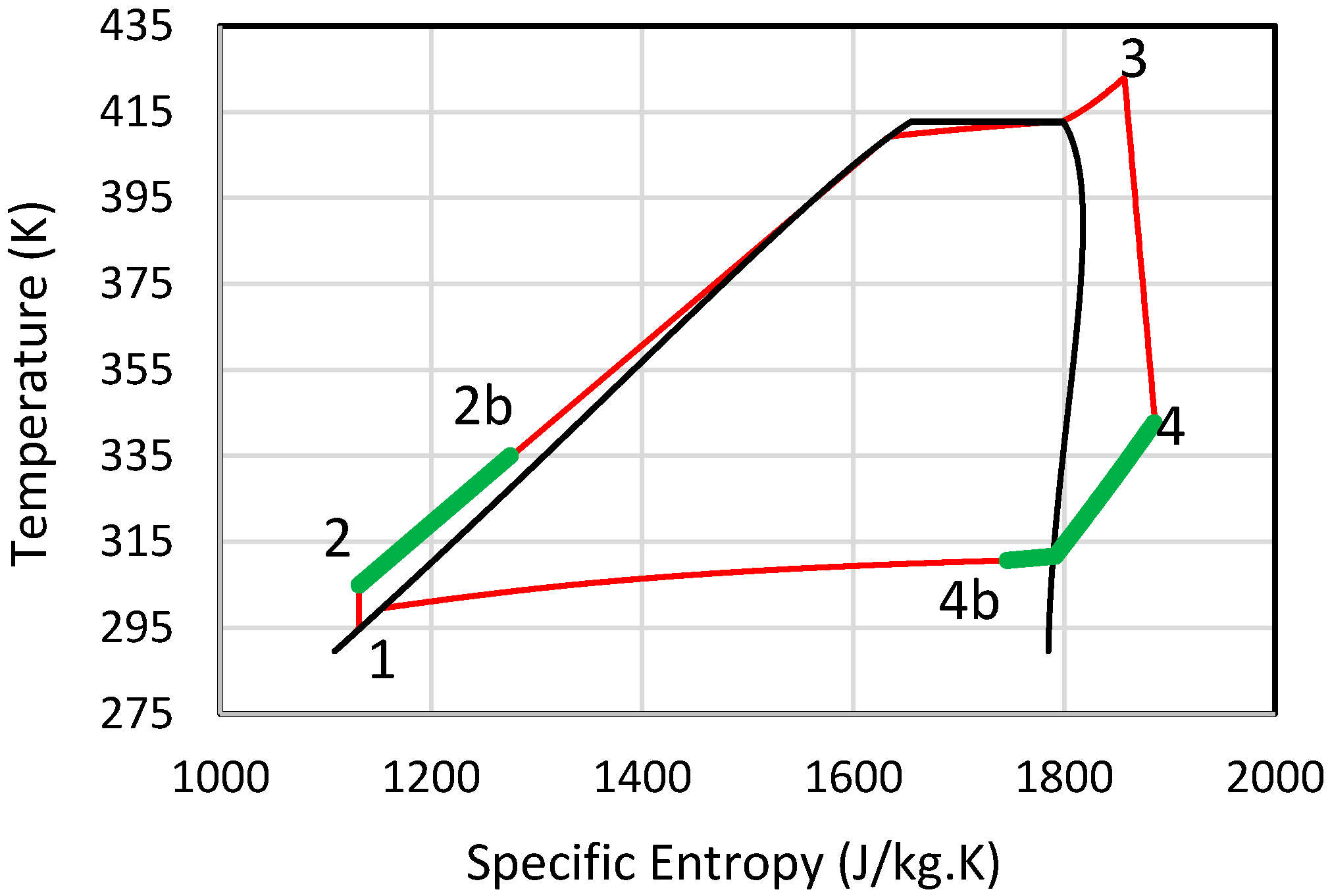
Figure 3.
Annual temperature variation and associated changes in working fluid composition for Beijing.
Figure 3.
Annual temperature variation and associated changes in working fluid composition for Beijing.
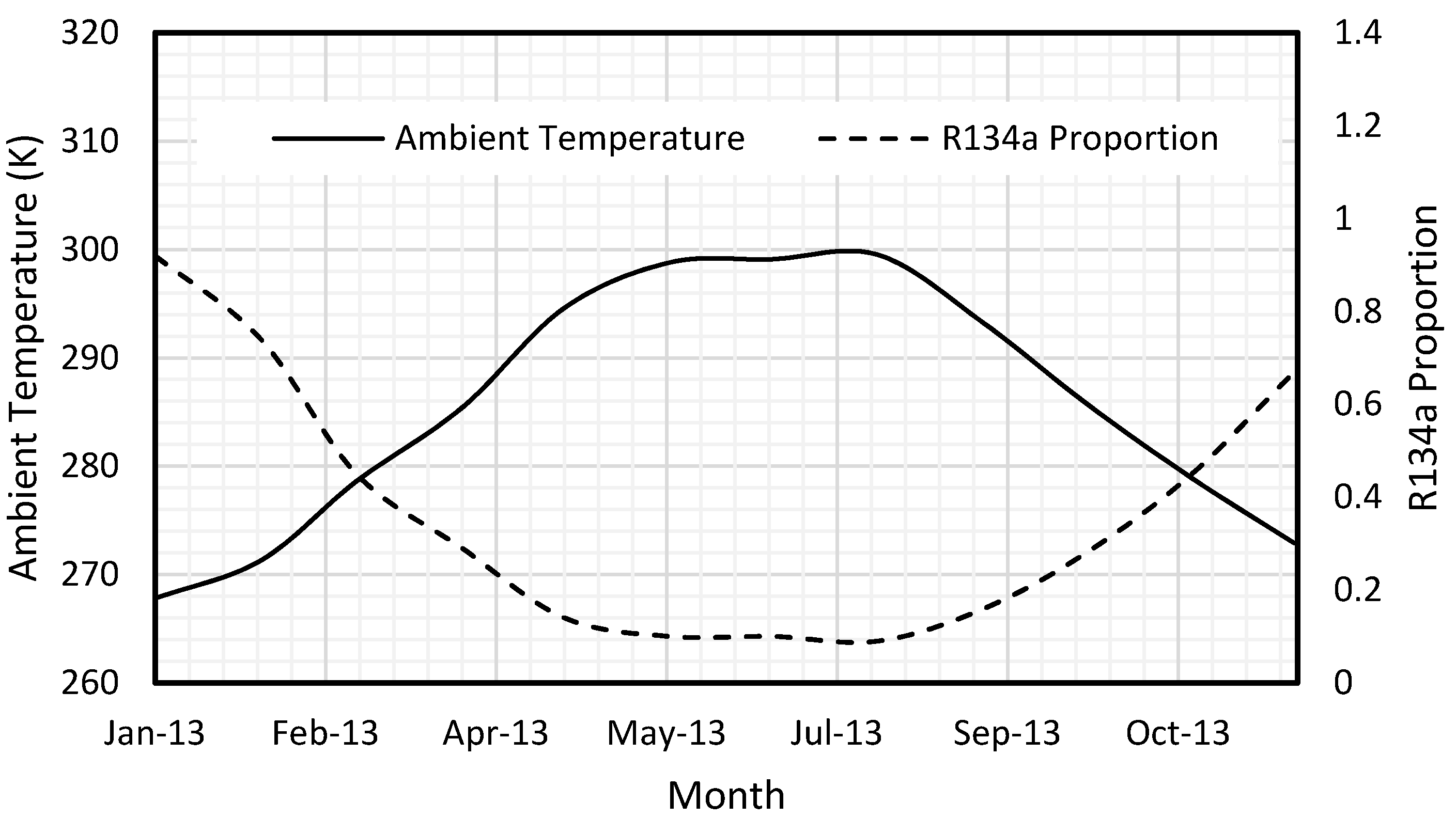
Figure 4.
Variation in Cycle Efficiency with ambient temperature for a heat source temperature of 100 °C under Beijing’s ambient conditions.
Figure 4.
Variation in Cycle Efficiency with ambient temperature for a heat source temperature of 100 °C under Beijing’s ambient conditions.
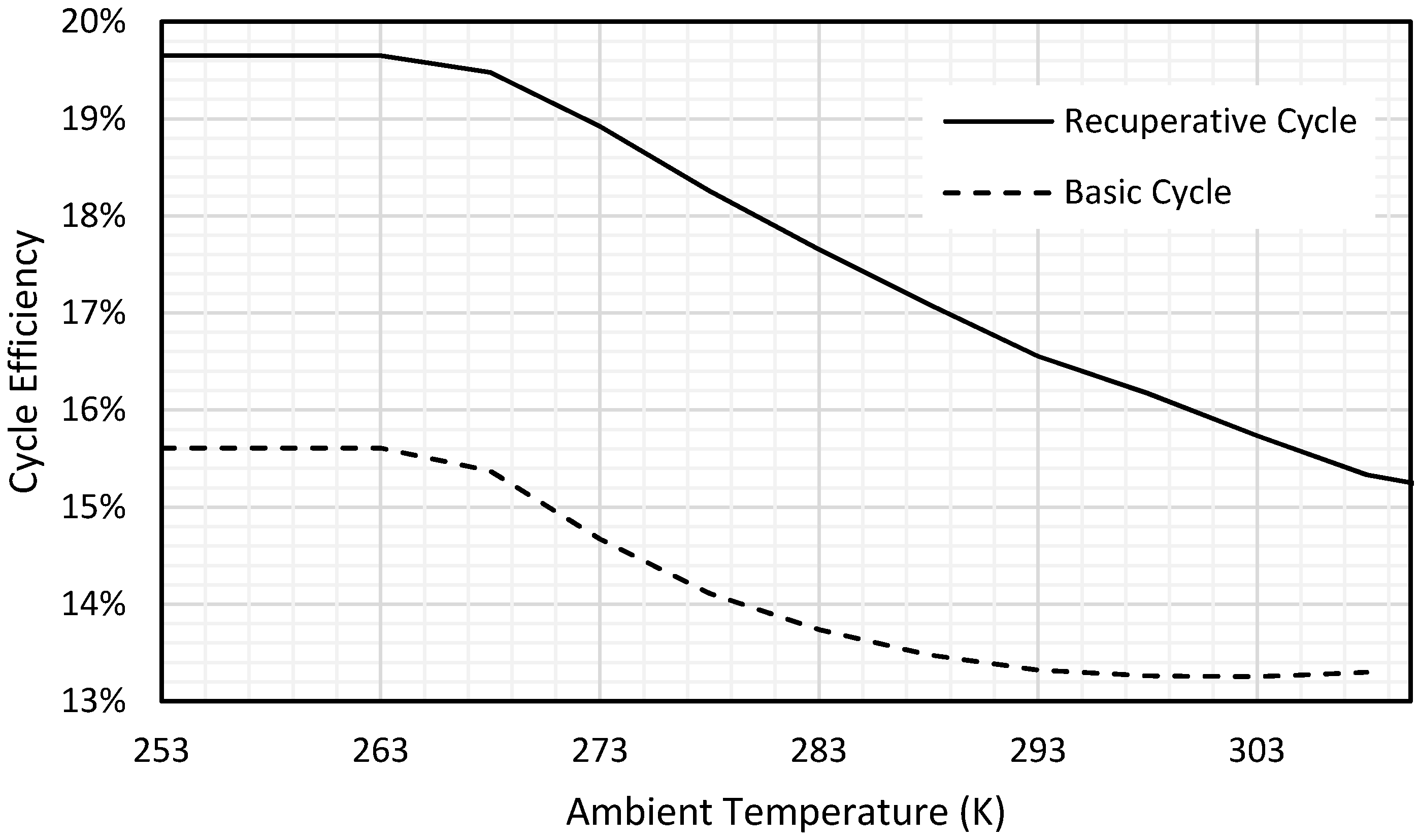
Figure 5.
Comparison of enthalpy change in each major cycle component with varying ambient temperature for a heat source temperature of 100 °C in Beijing’s ambient conditions.
Figure 5.
Comparison of enthalpy change in each major cycle component with varying ambient temperature for a heat source temperature of 100 °C in Beijing’s ambient conditions.
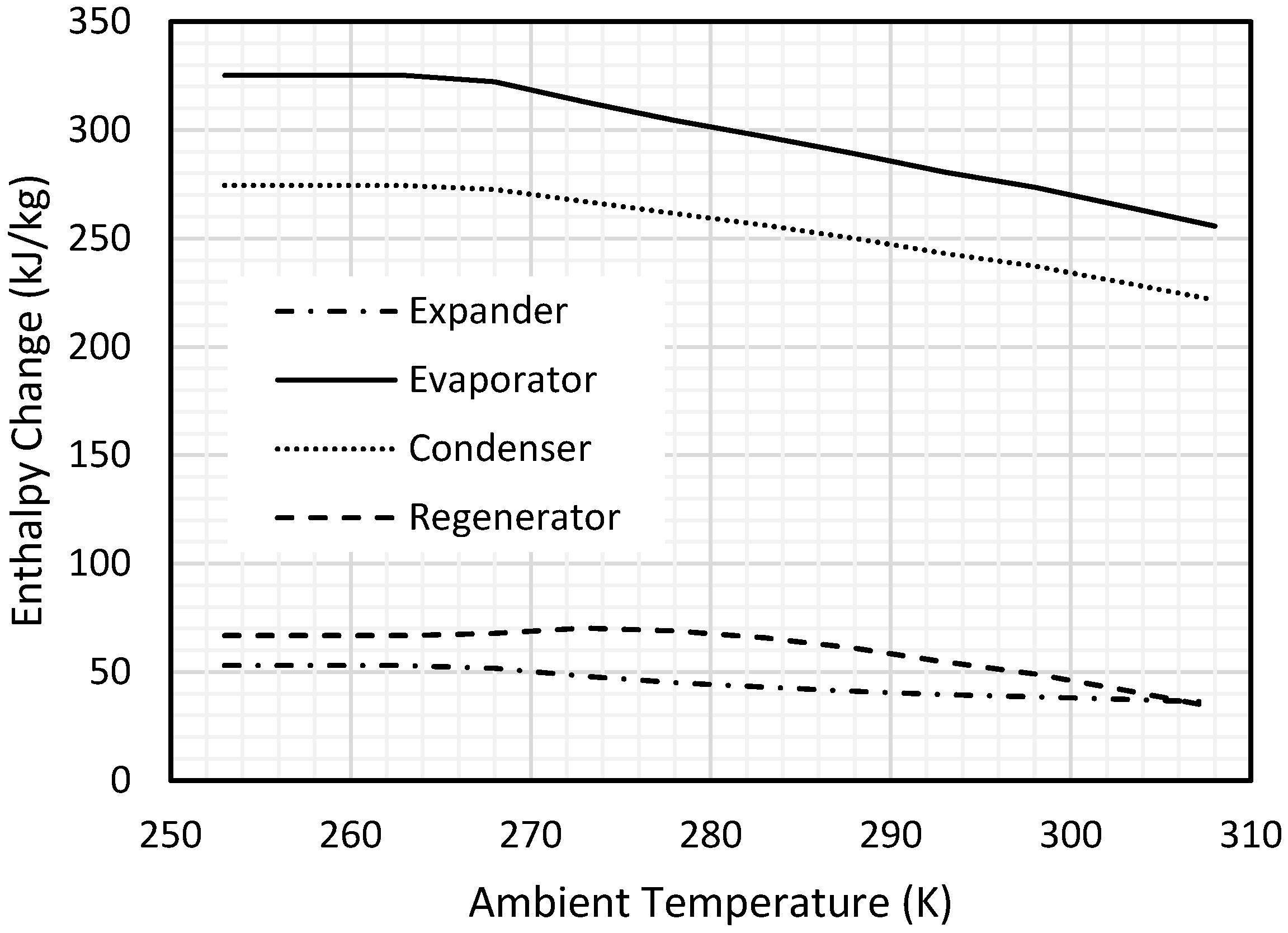
Figure 6.
Comparison of dynamic Organic Rankine Cycles operating under high temperature (290 K, left) and low temperature (265 K, right) ambient conditions.
Figure 6.
Comparison of dynamic Organic Rankine Cycles operating under high temperature (290 K, left) and low temperature (265 K, right) ambient conditions.
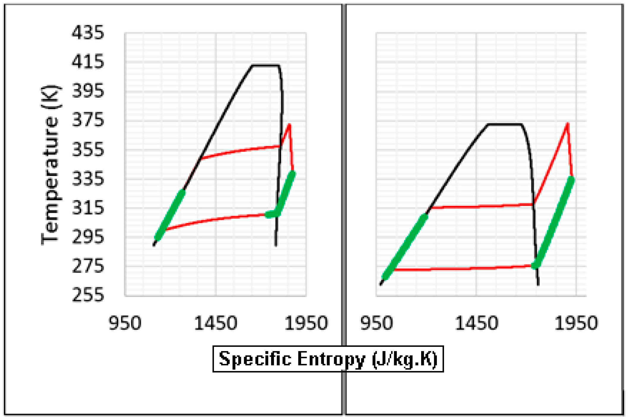
Figure 7.
Annual variation in cycle efficiency for a heat source temperature of 100 °C under Beijing’s ambient conditions. Graph shows monthly averages.
Figure 7.
Annual variation in cycle efficiency for a heat source temperature of 100 °C under Beijing’s ambient conditions. Graph shows monthly averages.
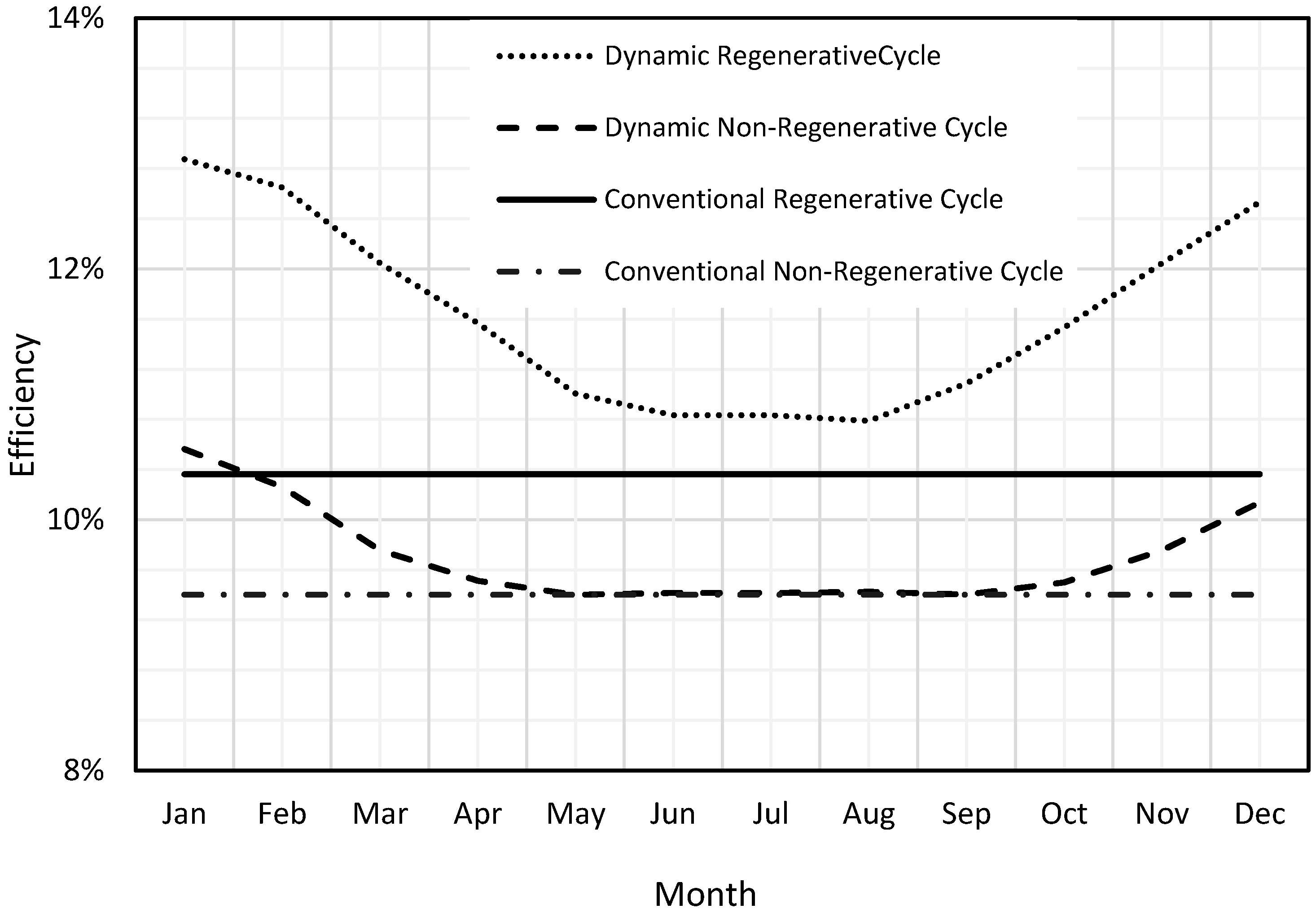
Figure 8.
Variation in ψ for five case studies for annual temperature variation. From left to right, Mumbai, Ushuaia, Glasgow, Phoenix, Beijing.
Figure 8.
Variation in ψ for five case studies for annual temperature variation. From left to right, Mumbai, Ushuaia, Glasgow, Phoenix, Beijing.
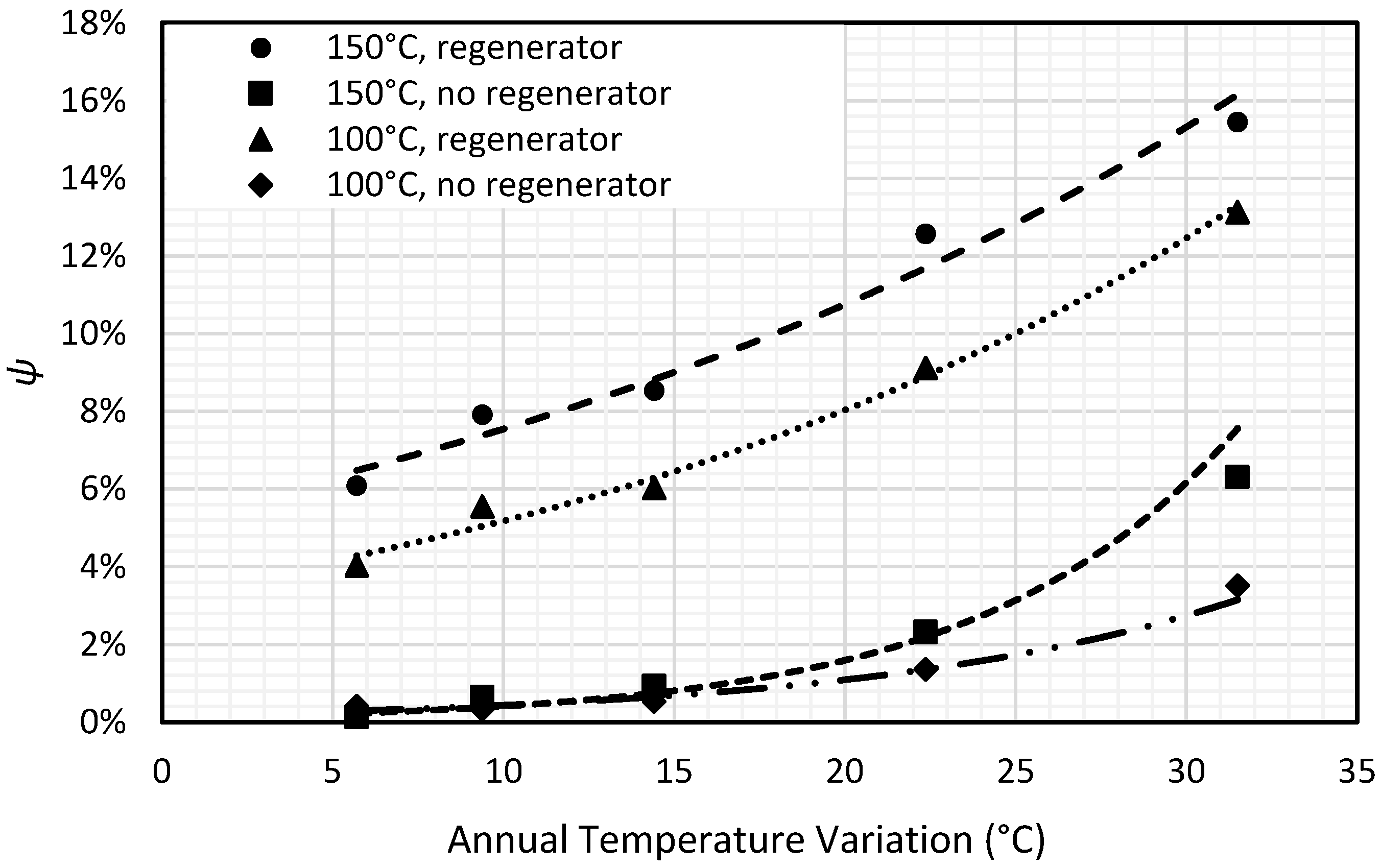
Figure 9.
Variation in ψ with changing heat source temperature under Beijing’s ambient conditions.
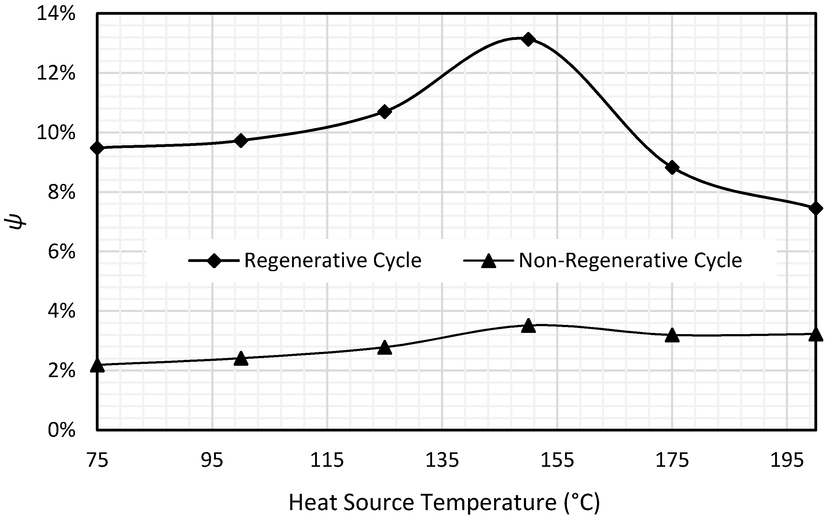
Figure 10.
Variation in Evaporator and Condenser pressure with changing heat source temperature for Beijing’s ambient conditions.
Figure 10.
Variation in Evaporator and Condenser pressure with changing heat source temperature for Beijing’s ambient conditions.
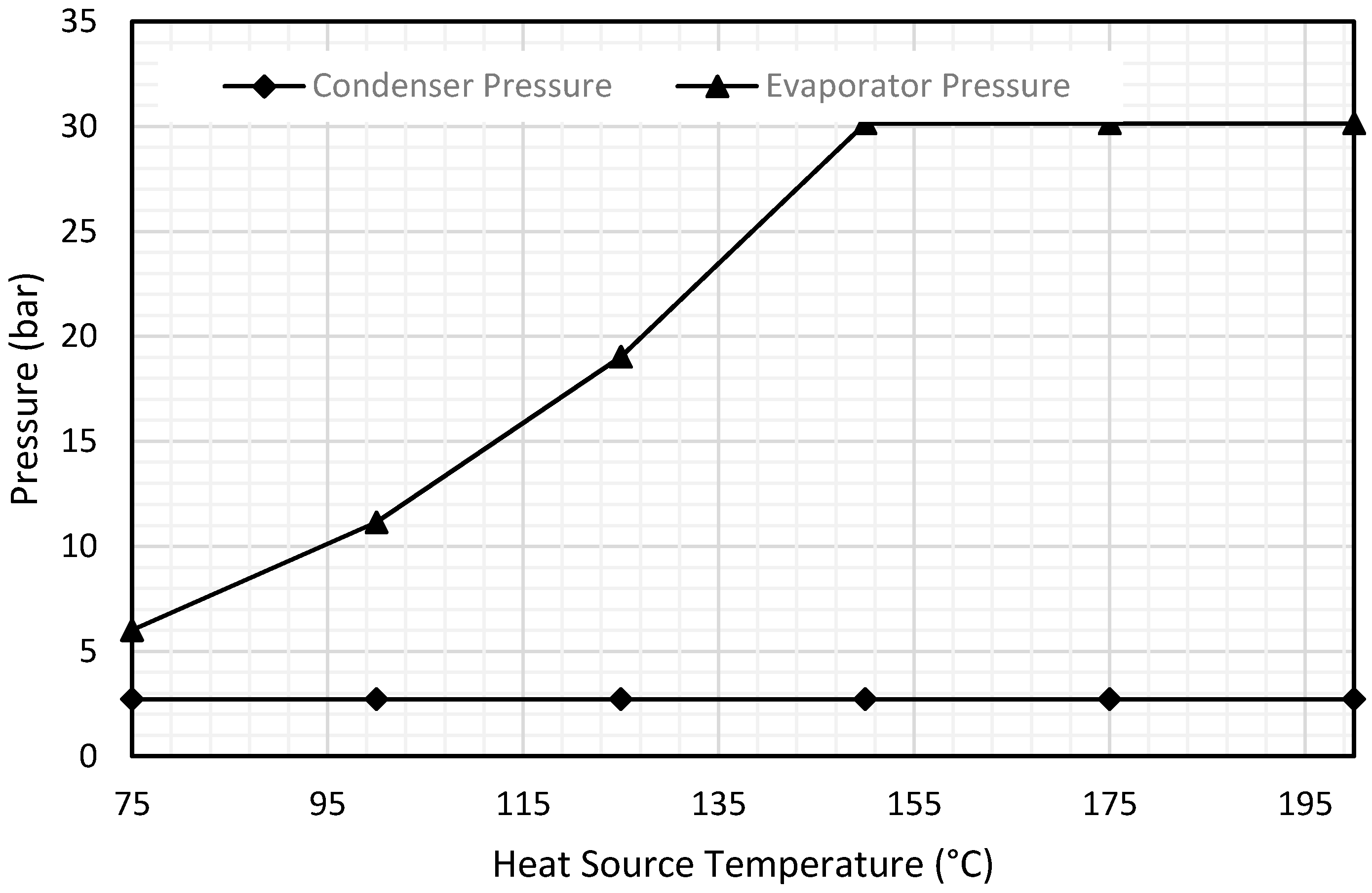
Figure 11.
Variation in specific power for recuperative and non-recuperative dynamic cycles over the course of the year for Beijing’s ambient conditions, and a heat source temperature of 100 °C. The specific power of the cycle does not vary depending on whether a recuperator is present, so these two curves are identical.

Figure 12.
Evaporator Pinch Point Diagrams for a heat source temperature of 100 °C and heat sink temperatures of −11 °C (left) and 25 °C (right).
Figure 12.
Evaporator Pinch Point Diagrams for a heat source temperature of 100 °C and heat sink temperatures of −11 °C (left) and 25 °C (right).
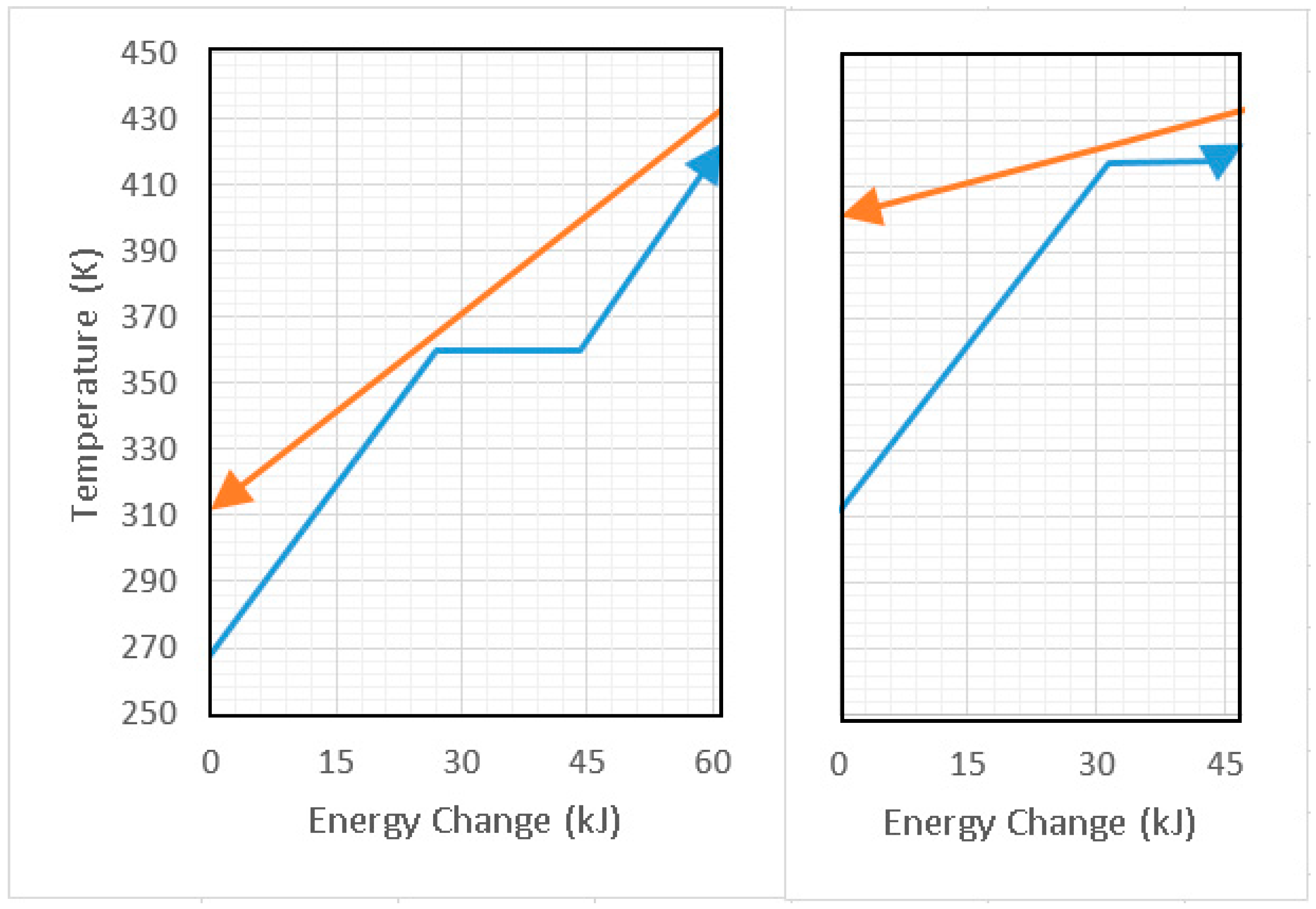
Figure 13.
Variation in ϕ with varying heat source temperature for Beijing’s ambient conditions.
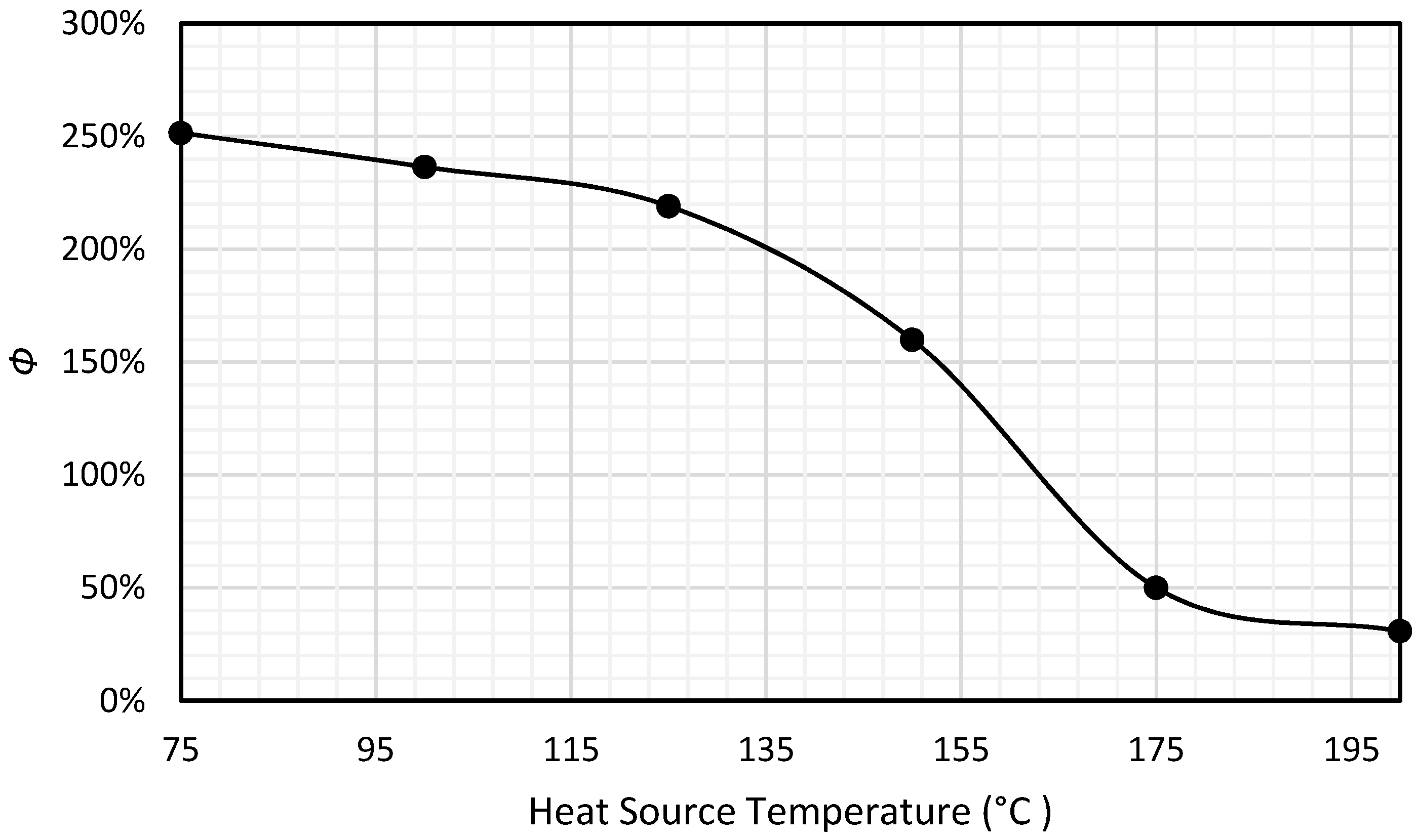
Figure 14.
Variation in the Specific Power of the Non-Dynamic Cycle with varying heat source temperature with Beijing’s ambient conditions.
Figure 14.
Variation in the Specific Power of the Non-Dynamic Cycle with varying heat source temperature with Beijing’s ambient conditions.
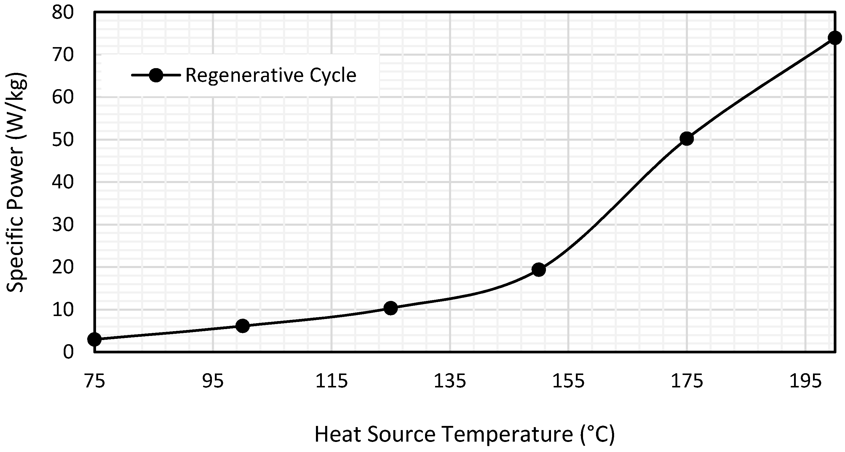
Figure 15.
Superheat at expander inlet over the course of the year for a heat source temperature of 75 °C under Beijing’s ambient conditions.
Figure 15.
Superheat at expander inlet over the course of the year for a heat source temperature of 75 °C under Beijing’s ambient conditions.

Figure 16.
Variation in exergy destruction in each cycle component over the course of the year for a heat source temperature of 75 °C with a recuperator.
Figure 16.
Variation in exergy destruction in each cycle component over the course of the year for a heat source temperature of 75 °C with a recuperator.

Figure 17.
Variation in exergy destruction in each cycle component over the course of the year for a heat source temperature of 75 °C without a recuperator.
Figure 17.
Variation in exergy destruction in each cycle component over the course of the year for a heat source temperature of 75 °C without a recuperator.
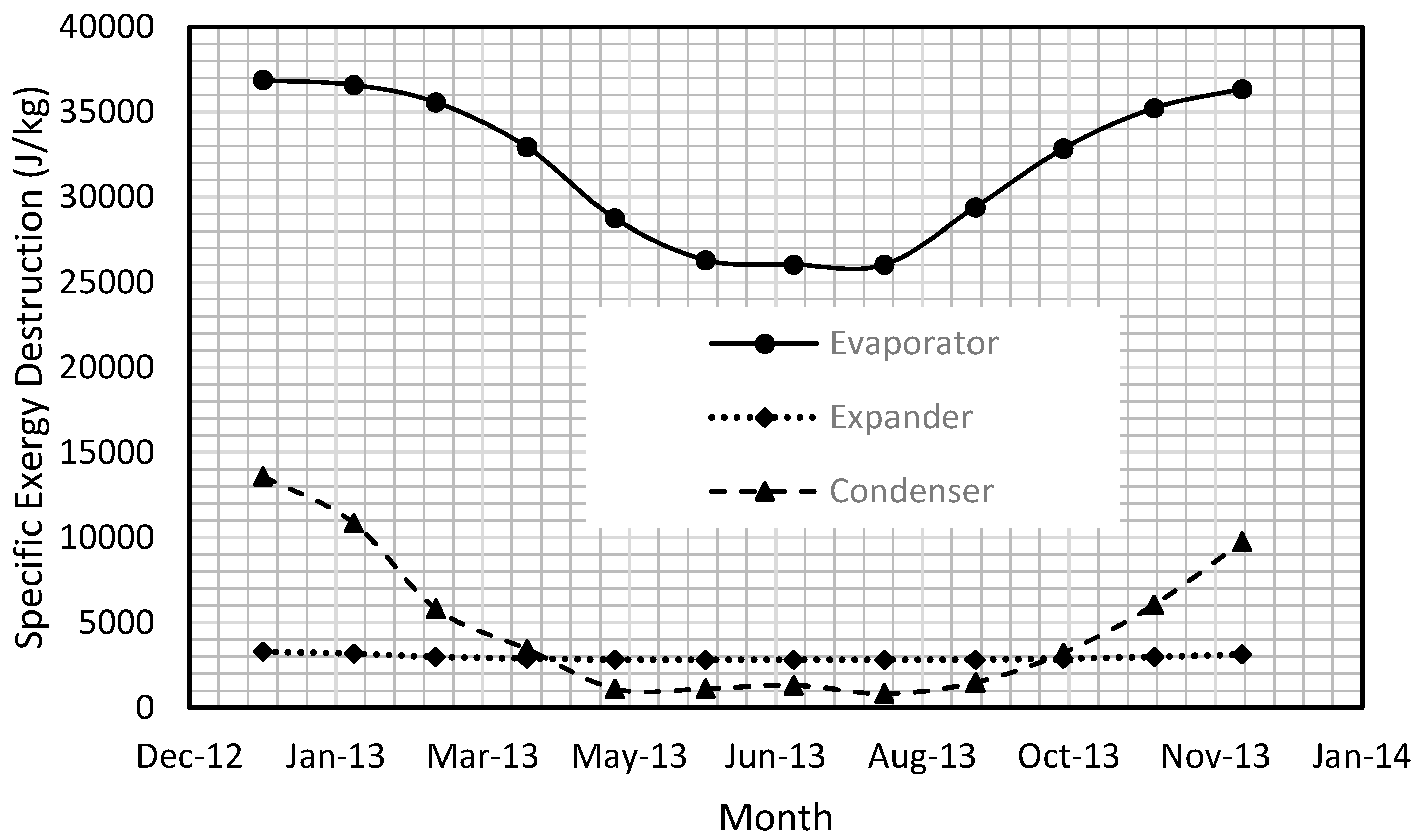
Figure 18.
Variation in Exergy Efficiency over the year for a heat source temperature of 75 °C under Beijing’s ambient conditions for the Recuperative, Non-Recuperative, and Conventional (Non-Dynamic) cycles.
Figure 18.
Variation in Exergy Efficiency over the year for a heat source temperature of 75 °C under Beijing’s ambient conditions for the Recuperative, Non-Recuperative, and Conventional (Non-Dynamic) cycles.
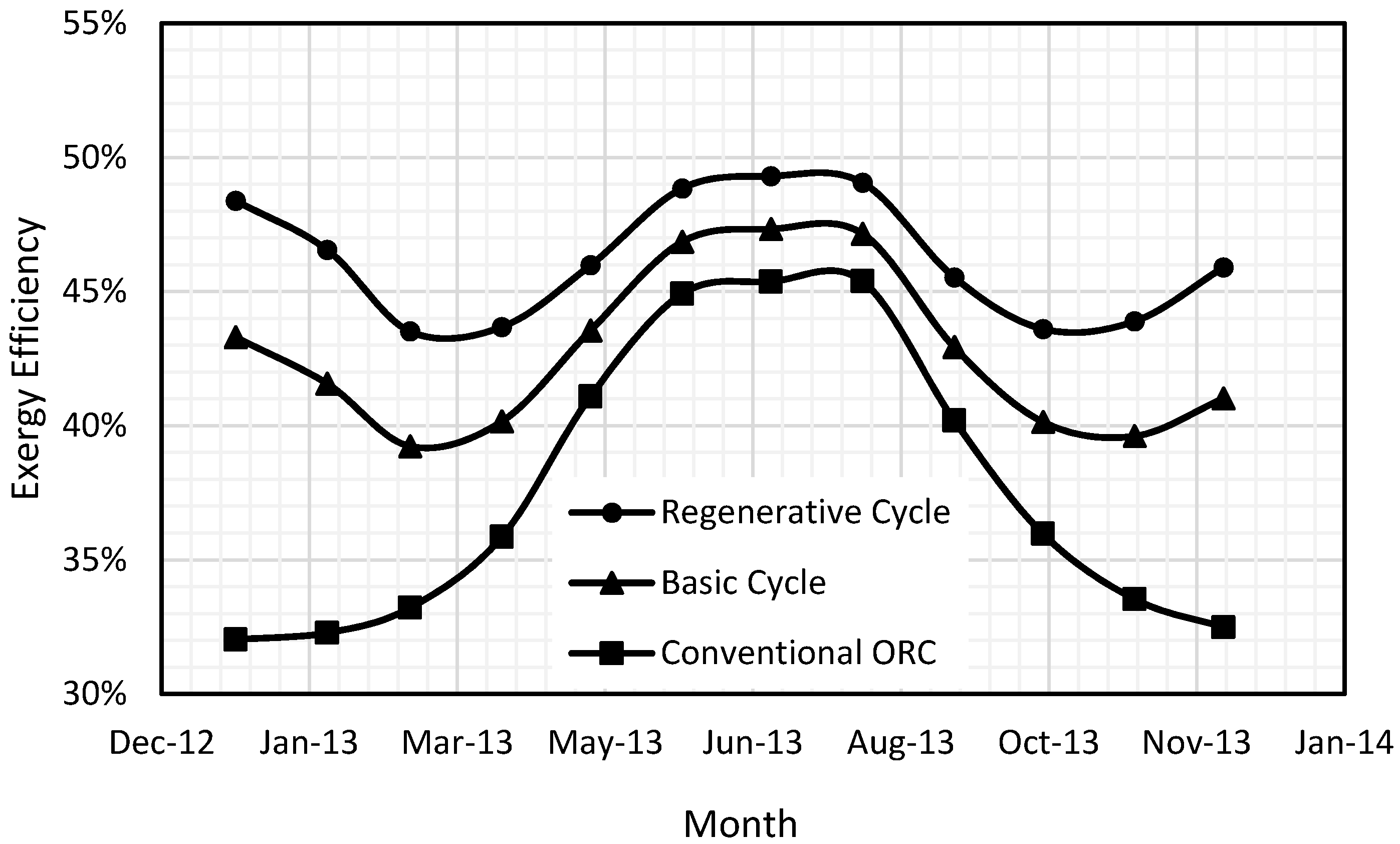
Figure 19.
Variation in Nusselt Number in the evaporator for a heat source temperature of 100 °C.
© 2017 by the authors. Licensee MDPI, Basel, Switzerland. This article is an open access article distributed under the terms and conditions of the Creative Commons Attribution (CC BY) license (http://creativecommons.org/licenses/by/4.0/).
Share and Cite
MDPI and ACS Style
Collings, P.; Yu, Z. Numerical Analysis of an Organic Rankine Cycle with Adjustable Working Fluid Composition, a Volumetric Expander and a Recuperator. Energies 2017, 10, 440. https://doi.org/10.3390/en10040440
AMA Style
Collings P, Yu Z. Numerical Analysis of an Organic Rankine Cycle with Adjustable Working Fluid Composition, a Volumetric Expander and a Recuperator. Energies. 2017; 10(4):440. https://doi.org/10.3390/en10040440
Chicago/Turabian StyleCollings, Peter, and Zhibin Yu. 2017. "Numerical Analysis of an Organic Rankine Cycle with Adjustable Working Fluid Composition, a Volumetric Expander and a Recuperator" Energies 10, no. 4: 440. https://doi.org/10.3390/en10040440
Note that from the first issue of 2016, this journal uses article numbers instead of page numbers. See further details here.