
Power Loss Analysis for Wind Power Grid Integration Based on Weibull Distribution

1
Groupe de Recherche en Electrotechnique et Automatique GREAH Lab., University of Le Havre, 76600 Le Havre, France
2
Laboratoire de Maitrise des Enregies Renouvelables, Faculty of Technology A. Mira University, 06000 Bejaia, Algeria
*
Author to whom correspondence should be addressed.
Energies 2017, 10(4), 463; https://doi.org/10.3390/en10040463
Submission received: 3 January 2017
/
Revised: 28 March 2017
/
Accepted: 29 March 2017
/
Published: 2 April 2017
(This article belongs to the Collection Wind Turbines)
Abstract
:The growth of electrical demand increases the need of renewable energy sources, such as wind energy, to meet that need. Electrical power losses are an important factor when wind farm location and size are selected. The capitalized cost of constant power losses during the life of a wind farm will continue to high levels. During the operation period, a method to determine if the losses meet the requirements of the design is significantly needed. This article presents a Simulink simulation of wind farm integration into the grid; the aim is to achieve a better understanding of wind variation impact on grid losses. The real power losses are set as a function of the annual variation, considering a Weibull distribution. An analytical method has been used to select the size and placement of a wind farm, taking into account active power loss reduction. It proposes a fast linear model estimation to find the optimal capacity of a wind farm based on DC power flow and graph theory. The results show that the analytical approach is capable of predicting the optimal size and location of wind turbines. Furthermore, it revealed that the annual variation of wind speed could have a strong effect on real power loss calculations. In addition to helping to improve utility efficiency, the proposed method can develop specific designs to speeding up integration of wind farms into grids.
1. Introduction
The structure, operation, and planning of electric power networks will undergo considerable and rapid changes due to increased global energy consumption. Therefore, electric utility companies are striving to install wind turbines as energy resources to meet growing customer load demand. In recent years, the installation of wind farms in electrical networks has provided numerous benefits: improving the environment, reducing energy losses, improving reliability, and stabilizing energy prices [1].
Since wind turbine units have a small capacity compared to conventional power plants, its impact is minor if the penetration level is low (1%–5%). However, if the penetration level of wind farms increases to the anticipated level of 20%–30%, they will have a high impact on the active power loss of the grid [2]. A simple analysis method for determining the real losses considering the wind resource has been implemented by [3]. It is based on DC power flow, while certain errors in calculation are observed when simulated running in AC power flow for several wind conditions. In [4], the point estimate method (PEM) was used as an assessment of the operational risk in electrical distribution systems. A hybrid genetic algorithm (HGA) is employed to reduce network losses, improved voltage profiles, and reduce total costs of system operation planning associated with distributed generators (DGs).
The wind farm can be helpful at the margin in providing clean power. Determining the capacity of the wind farm into electrical networks is the most challenging part for most utilities. The improper allocation of wind farms would lead to increasing the losses in the power system more than without a wind farm. Therefore, many researchers have proposed different approaches to evaluate the proper placement and sizing of wind turbines in electrical networks [5]. Multi-objective optimization problems (MOP) and game optimization theory (GOT) were used in selecting the optimal size and site of DGs in [6]. The distribution system planning (DSP) issues, such as costs, losses, and voltage index, have been considered as objective functions. In recent years, the development of computers has created a trend of using various stochastic optimization techniques for active power analysis. The Jaya algorithm [7] has been implemented for three goal functions: loss reduction, improvement of voltage stability, and minimization of generation cost. However, this optimization technique is based on environment and economic power dispatch as an objective function.
The impact of renewable resources (as distributed generation, DG) on a distribution network with several numbers of important issues (system voltage, protection loss of the power grid, system restoration, and network) has been discussed [8]. A case study assessed the impact of the connection of significant amounts of DGs on energy losses and voltage drops in the distribution system [9]. To solve the problem of optimal size and allocation of DGs, researchers have employed conventional analytical approaches using sensitivity factors obtained from quantities, such as the system bus impedance and admittance matrices, and the exact loss formula [10,11,12]. Efficient methods, based on the load concentration factor (LCF), and an improved analytical (IA) method have been compared to select the optimal DG placement in order to reduce losses [13].
The impact of wind energy integration on voltage stability by using the Flexible AC Transmission System (FACTS) has been presented [14,15]. The injection of reactive power into the grid (controlled by the thyristor firing angle) was considered as a state variable in the power flow calculation. The FACTS has been used to provide the reactive power to control and optimize the voltage.
Increasing the wind power penetration level was interesting for different researchers. The wind power development and the financial risk for its investors in Denmark, Germany, Spain, and Ireland has been discussed [16]. In the UK, The Netherlands, and Germany, a nine-node DC network has been investigated to minimize the transmission losses by using a genetic algorithm (GA) [17]. The fault ride-through and voltage maintenance of the grid has been considered for the integration of wind turbines into the German transmission system [18]. In [19], the Spanish transmission system with wind farm behavior has been discussed to confirm the verification, validation, and certification procedure.
The uncertain parameters (technical and economical) can play an important role in modelling renewable distributed generation. Authors in [20] attempted to provide a state-of-the-art review regarding stochastic techniques for uncertainty modeling. Different models (robust optimization, interval analysis, probabilistic, and hybrid methods) have been compared to investigate their strengths and shortcomings.
Due to wind speed variations, various nonlinear losses in wind turbines, transmission lines, and interconnection grids changed and, consequently, so did the efficiency of the power system. The iron losses, copper losses, mechanical losses, converter loss, stray load loss, and efficiency of energy can be calculated as a function of wind speed with no approximation required [21]. However, this paper aims to speed up the calculation based on the approximation of DC power flow and all of these losses will be neglected.
High levels of variable electricity generation produced by renewable resources need flexibility of calculation with less time to improve the stability, reliability, and economy [22]. The computer execution time is an important factor for many of the utilities, but none of these studies considers it. However, the research goals must take into account the impact of wind speed on power loss calculations.
The goal of this paper is to reveal that the annual variation of wind speed could have a strong effect on real power loss calculations. The methodology considers a model of wind resources according to a probability distribution (Weibull statistic). In addition, an analytical study has been developed for speeding up the integration of a wind farm into a power grid by selecting its size and placement, taking into account the reduction of total active power loss. In brief, these methods have an analytical approach and Simulink simulation, and it is focuses on the real power loss calculation as a function of the wind resource.
This paper is organized as follows: first, Section 2 describes the wind farm model. Next, power flow and graph theory for electrical network modeling, and then the power loss calculation was applied to find the optimal size and placement of the wind farm at each bus of the system in Section 3. Finally, the selection of the size and placement of the wind farm, in addition to the results, are provided in Section 4 and Section 5, respectively. Finally, the conclusions are described in Section 6.
2. Wind Farm Model
The actual mechanical power output () extracted from wind can be written as;
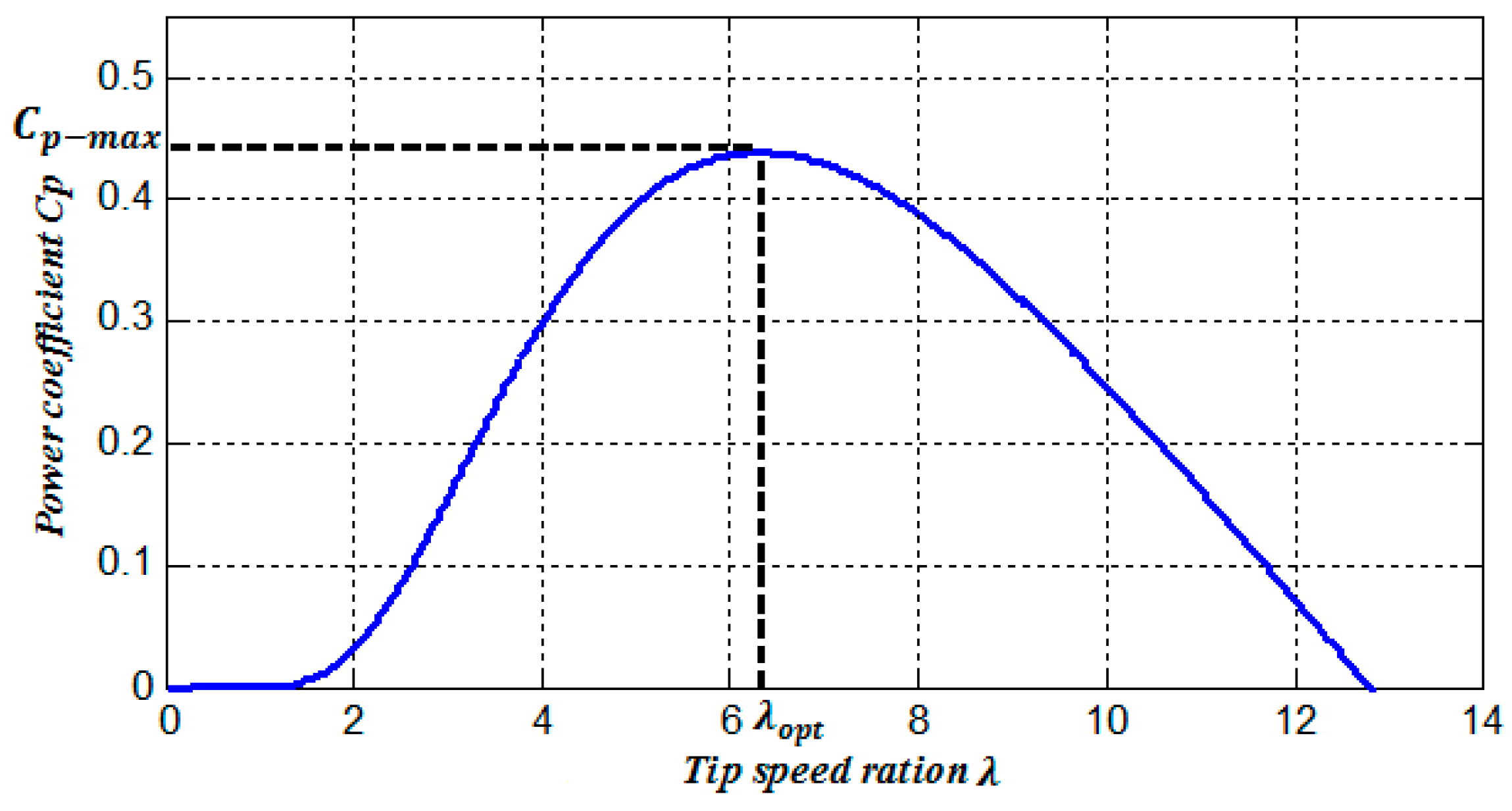
where is the air density (kg/m3), is the blade radius of the wind turbine (m), is the wind speed (m/s), and is the power coefficient. The power coefficient varies with the speed of the wind, the rotation speed of the turbine, and the turbine blade parameters. Therefore, is a function of the tip speed ratio and the blade pitch angle . has been approximated using the following function:
where:
Figure 1 shows the calculated relationship between the power coefficient and the tip-speed ratio for pitch angle .
The tip speed ratio is expressed as:
where is the wind turbine rotation. The turbine torque is the ratio of the output power to the shaft speed:
The turbine is normally coupled to the generator shaft through a gearbox whose gear ratio is chosen in order to set the generator shaft speed within a desired speed range. Neglecting the transmission losses, the torque and shaft speed of the wind turbine, referring to the turbine-side of the gearbox, are given by:
where and are, respectively, the turbine and generator torques.
The optimal mechanical power, which can be generated using the maximum power point tracking (MPPT), can be expressed as:
A wind turbine model with speed control is shows in Figure 2.
The wind farm has been represented as an active generator in power flow studies. This active power generator will be added into the grid only at load buses. The output electrical power generation is given by:
where , , and are the cut-in speed, cut-out speed, and nominal speed of the wind turbine, respectively. is the rated output power of the turbine and is the average wind speed.
The wind farm consists of multiple wind turbines connected to the power grid through a transformer. In this study, doubly-fed induction generators (DFIG) have been selected as the wind turbine generation systems, as shown in Figure 3. This DFIG configuration is very attractive from an economical point of view because it uses a smaller frequency converter, which compensates for the reactive power consumed by the power electronics equipment.
This section is divided by subheadings, which should provide a concise and precise description of the Simulink results, their interpretation, as well as the experimental conclusions that can be drawn.
3. Analytical Approach
3.1. DC Power Flow
Let us consider a π-model of a transmission line (k to m). In a per unit system, the voltage magnitude throughout any power network is relatively close to unity during light load conditions:
where:
- : is the voltage magnitude at bus k.
- : is the voltage magnitude at bus m.
For most typical operating conditions, the difference in angles of the voltages at two buses k and m connected by a circuit, which is − for buses k and m, is less than 10–15 degrees. It is extremely rare to see such angular separation exceed 30 degrees. Thus, it can be considered that:
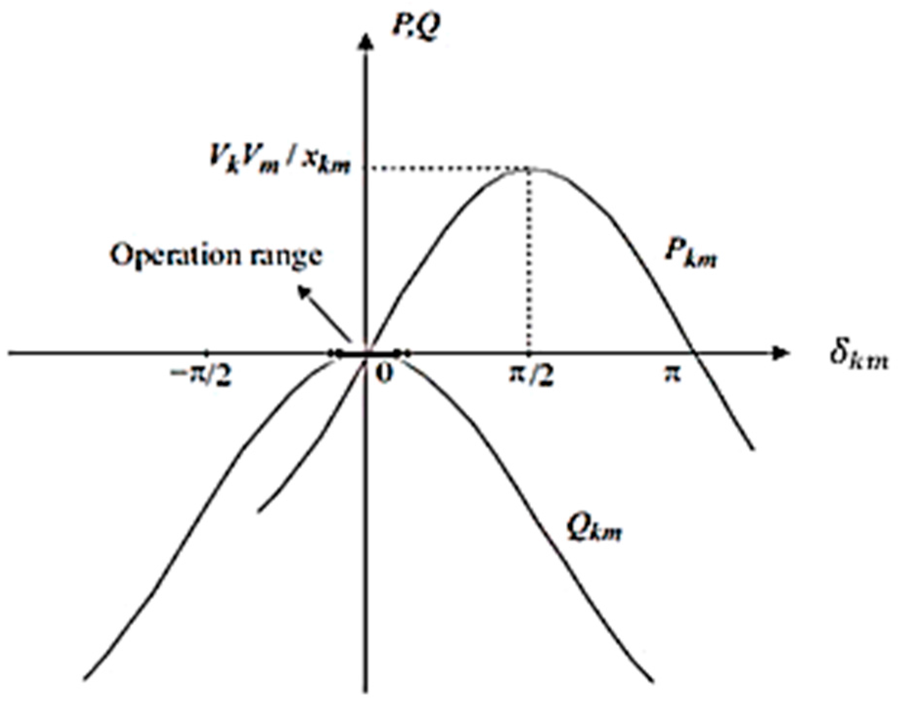
In the usual range of operations, a strong coupling between active power and the voltage angle, as well as between reactive power and voltage magnitudes, exists, while a much weaker coupling between the reactive power and voltage angle, and between the voltage magnitude and active power, exists, as shown in Figure 4.
Based on the above, the AC power flow in the lines can be approximated and linearized by neglecting the imaginary part of the system (reactive power) where R << X, voltage magnitude of buses are set to 1.0 per unit, and the voltage angle is assumed to be small. The active power () injections in buses can be derived and calculated by multiplying the nodal admittance matrix () by the angles () of the buses as follows [23]:
while the active power flow through transmission line can be calculated by multiplying non-diagonal elements of negative susceptance by the difference between the voltage angles of the two line terminals as:
where:
- is the vector of power flow which has dimension (M × 1).
- D is the vector (M × 1) or diagonal matrix (M × M) elements, which is formed by placing the negative susceptance (−).
- is the vector of the voltage angles of buses (N − 1 × 1).
- At is the incidence matrix (M × N − 1) between the node (voltage angle) and the arc (voltage angles differences).
The AC power flow is linearized to be the DC power flow based on three assumptions. The first assumes that the resistance of the line is negligible compared to its reactance, which means a low R/X ratio. This assumption is more applicable for transmission lines with a high voltage level and for R/X ratios below 0.5. The average error will be smaller than 5% and 2% for R/X ratios below 0.5 and 0.2, respectively [24]. The second assumption is that differences of the voltage angle are small, especially between neighboring nodes. This assumption practically corrects during peak load in a mesh grid and mostly in the weakly-loaded grid. Note that the voltage angle difference will be between a small number of lines, and the error of the sine and cosine terms made by linearization is less than 1% for 6 degrees. The third simplification assumes the voltage magnitudes are at unity and not fluctuating. In general, this assumption can create an average error of 5% for voltage deviations less than 0.01 p.u. In general, the average error between the accuracy of DC and AC power flows will be acceptable and not exceed 5% in high voltage grids. However, this error will be much larger for single-line flows in radial systems and actual power systems with realistic voltage fluctuations.
3.2. Graph Theory and Incidence Matrix
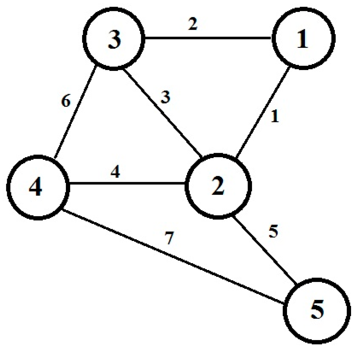
The power system is converted to a graph G(V, E), where V represents the set of vertices or nodes (buses in the network) and E represents arcs (interconnection lines among buses in the network) [25]. Figure 5 and Figure 6 show an example of a five-bus system (adopted in this work) and its direct graph representation.
The incidence matrix (A) of a graph G is a (M × N − 1) matrix that shows the relationship between the nodes and arcs, where M and N − 1 are the numbers of lines and buses, respectively. This matrix contains a number of rows equal to the number of arcs and a number of columns equal to the number of nodes. Note that it has only N − 1 columns because the angle of the reference bus is being set equal to zero.
The incidence matrix (A) can be expressed mathematically as follows:
For the five-bus system above, the incidence matrix will be:
3.3. Power Loss of the Wind Farm Integration Grid
From Equations (11) and (12), the power flow is a function of power injections as follows:
while the power injections can be expressed as:
where and are the active power output of the m generators (the reference generator is not included) and the wind farm (with a vector (m × 1) of zero, except the wind farm bus), respectively. Note that the total number of generators is N, so the power output of the generators can be considered as:
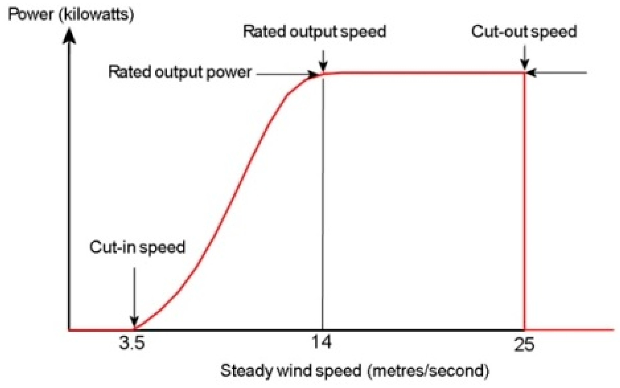
The total annual energy produced by the wind farm is a function of wind speed, which is mostly represented by a Weibull probability distribution. This distribution is used to estimate the total yearly average power output by combining the power produced with hours at any wind speed. Figure 7 illustrates an example of the relation between wind speed and its hours per year, according to the Weibull statistic [26].
According to this statistic, time of wind speed can be divided into three categories of duration:
For Figure 8, is the duration when the wind speed is less than the cut-in speed (between 2.5 to 3 m/s), is the duration when the wind speed is between the cut-in and the rated speed (10 m/s to 16 m/s), is the duration when the wind speed is between the rated speed and the cut-out speed (20 to 25 m/s), and when wind speed exceeds the cut-out speed. That means the total annual duration is:
Aggregating the wind power output and duration of annual wind speed from Equations (8) and (19), respectively, the annual output energy of wind farm will be calculated as:
where:
Annual Energy = Power output (PW) × annual duration (Δt)
and are zero power output when the wind speed is less than the cut-in speed or more than the cut-out speed, respectively.
is the power output less than the rated power and its value changes when the wind speed changes.
is the rated power of the wind farm when the wind speed is greater than the rated wind speed and less than the cut-out speed.
This paper is concerned with the active or real power losses which are more affected by the wind farm. The total real power losses can be expressed as a function of wind farm output and it will have three values, two of them remain constant, while the third one will increase or decrease corresponding to a wind speed pattern.
At any line, losses across the series impedance of a transmission line are [27]:
Most of the wind turbines are represented by the active power generation so that reactive power flow can be neglected. In addition, voltage values at each bus are around 1 p.u., which can simplify the equation of real power loss as follows:
and with the wind farm output, it will be:
where the power losses for and are constant as follows:
While variable power loss between the cut-in and rated wind speeds can be written as:
The total real power losses as a function of the rated wind power output is:
4. Size and Placement Selection of Wind Fram
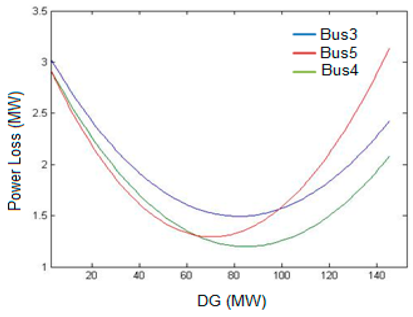
Firstly, the five-bus IEEE standard system has been tested with a linear load flow method to calculate the total real power losses without the wind farm. These calculations correspond to the power losses at duration (where the wind farm has zero output). Then, it has been repeated by adding the wind farm inside this system at different locations at load buses. At each location, the capacity of the wind farm was initiated with 1 MW power at the beginning, then it increases by 1 MW steps until it reaches 30% of total generation required for the whole system. Figure 9 shows the power loss variation with the total wind farm power for three different locations of the farm. However, these are approximate optimal values for the wind farm capacity because the reactive power flow in the lines was ignored, all voltage values were assumed to be 1 p.u., and an approximation method to calculate real power flows was used. The procedure presented in this paper has smooth properties, which leads to a solution close to the optimal values with fewer iterations, less memory use, and lower computation times. In addition, the error from the linearization method can be reduced during the estimation process.
The figure shows that for each location (bus), curves will have similar behavior, which can be divided into two parts. In the first part, the curves are close to linear and the losses will be decreased at each MW step of the wind farm until it reaches the minimum value. Then, curve behavior will be nonlinear in the second part, where the losses will increase when the wind farm output continues increasing. In the linear part, the curves of the losses will continue decreasing in parallel, but will sometimes intersect each other at the non-linear part.
The procedure begins to compute the total real power losses in lines before adding wind turbines, which will be located in different load buses. After adding the small amount of power (1 MW at the first load bus), the power flow computation is based on the proposed linear method and obtains the initial power loss by the simplified real power loss calculation. Then, the information of the individual power loss corresponding to the wind farm capacity (increased in 1 MW steps) are stored in PLosses, n, and in, respectively. The capacity and location of wind turbines will be selected by comparing the minimum value of these losses in stored memory.
Finally, the accumulated data of the minimum power loss, location, and size of the wind turbines are obtained. It is observed that each state converges sufficiently for different systems and it can predict the optimal size and location of wind farms for minimum losses. The time reduction and memory consumption required by the proposed linear model will help control centers of utilities by providing real-time data.
5. Results
5.1. Analytical Model Results
Before the wind farm is integrated into the five-bus IEEE system, a linear method has been implemented to calculate the total real power loss for the system. All generation units, load demand, and power loss are calculated and shown in Table 1.
From Figure 9, it is observed that bus 5 has minimum real power losses and it can be selected as the optimal placement of the wind farm. In addition, it is noted that increasing MW continues to decrease the real power losses by more than 50 MW. Thus, the capacity of the wind farm will be selected based on this condition (30% of total generation required), which is 45 MW, so the wind farm will consist of 30 individual wind turbines with rated output power of 1.5 MW and each of them will be subject to same distributed wind field.
The wind farm output power has two constant values, zero (MW), when the wind speed is less than the cut-in speed (3 m/s), and rated power output (1.5 MW), when the wind speed is between the rated (11 m/s) and cut-out (25 m/s) speeds. In addition, the variable values when the wind speed is varying between the cut-in and rated speeds can be determined by subtracting the losses from the mechanical power by Equation (1), according to the speed variation in Figure 7.
The real power loss for the five-bus IEEE system with wind farm penetration has been calculated for four durations (, , , ) to determine the average value, taking into account the variation of annual wind speed. Table 2 shows the real power output of wind farms and total real losses for three constant value durations (, , ) in addition to the variation in the value when the wind speed is between the cut-in and rated speeds. It is noted that the percentage differences between the yearly averages of real power losses and losses calculated for the rated wind farm is 37% for the five- bus IEEE system. The time consumption with the proposed method is less than 5 ms, which is performed on a computer with core i7-4800MQ CPU, 2.7 GHz, 16 GB RAM, and Microsoft Windows 7 operating system running in real-time mode.
5.2. Simulink Simulation Results
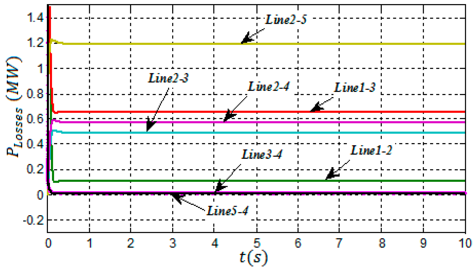
In order to validate the proposed analytical model, the five-bus IEEE modelling has been developed with Simulink. The wind farm (45 MW) is represented by five groups, each one has six wind turbines with a rated output power of 1.5 MW. The output power provided by the wind farm will vary due to the wind speed variations as shown in Figure 7. Firstly, the real power flow at each line (seven lines) in the system has been measured before integration of the wind farm. This measurement has been compared with more accurate calculations by the Newton Raphson method to validate the Simulink model, as in Figure 10. Then, the real power losses have been measured at each line to calculate the total losses in the system (3.07 MW) as shown in Figure 11. This calculation has been considered at the steady-state of the system and at constant loads.
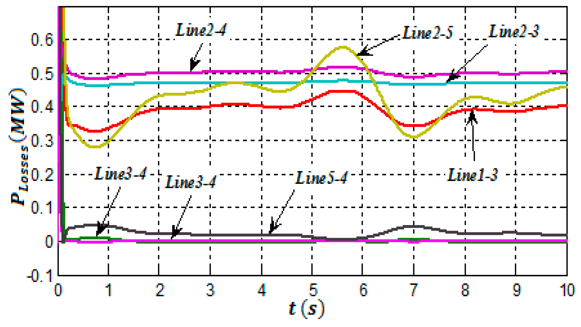
After connecting the wind farm into the five-bus IEEE system, the power flow, as well as the power losses into lines, will vary due to the wind power output variation, as shown in Figure 12 and Figure 13. The wind farm power output follows the same wind speed variation (Figure 7) applied in the analytical model.
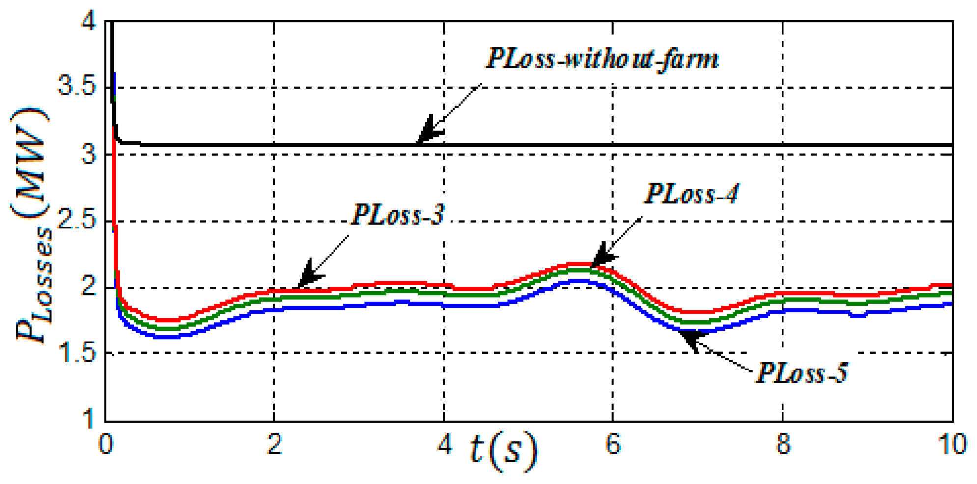
The location of the wind farm inside the grid has been changed to evaluate the real power losses in each case. It is proved that the injection of wind farm power output into bus 5 will minimize the total power losses more than other locations. The variation of real power losses was between 1.1 and 2.1 MW, while the average of it will be approximately 1.25 MW, as shown in Figure 14.
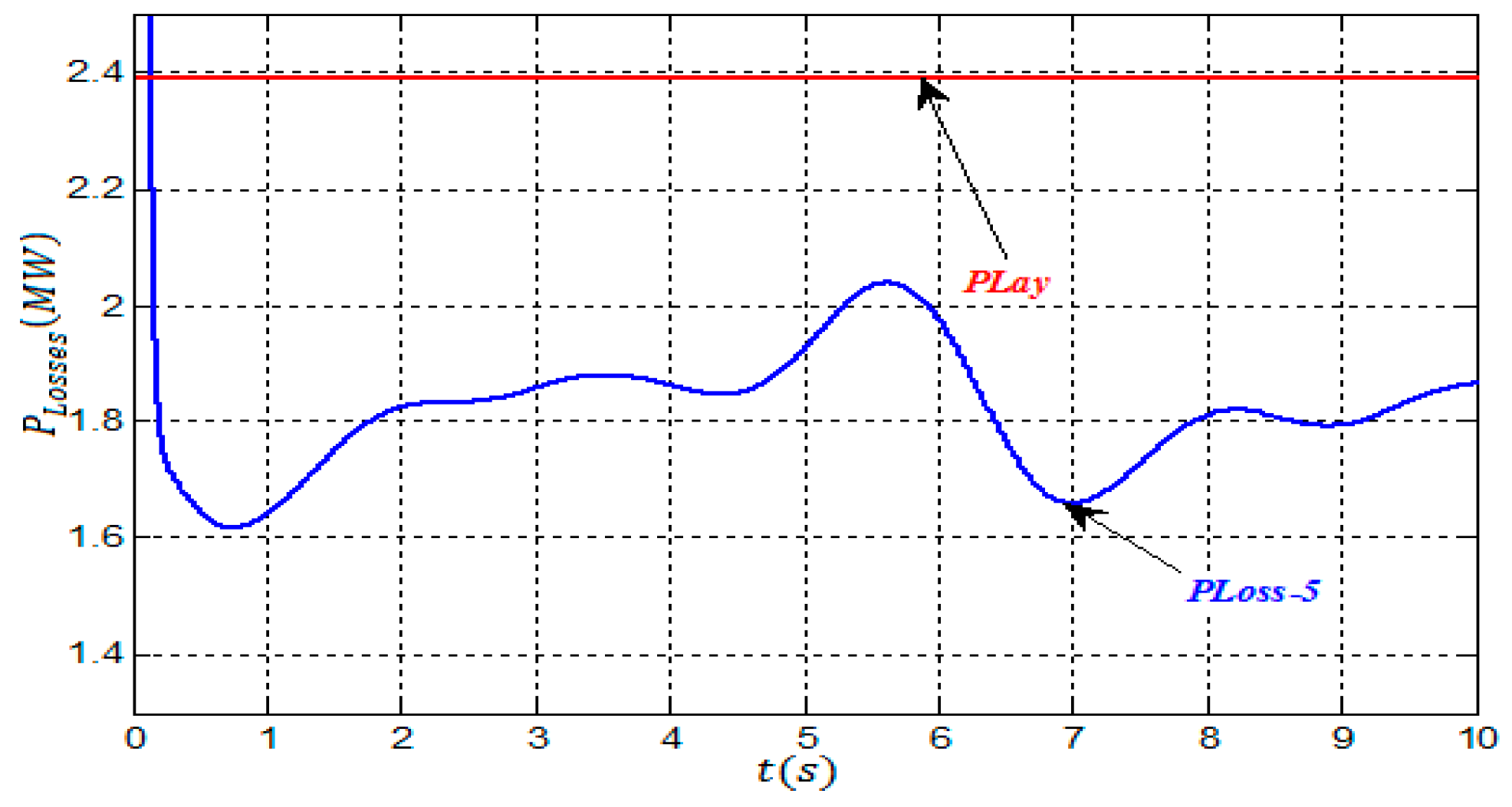
The annual average real power losses for the five-bus system is shown in Figure 15. PLay represents the average power losses per year calculated by the analytical method, while PLoss-5 represents the total power losses into the grid, taking into account changeable wind speeds during a certain period by Simulink.
6. Summary
Under actual operating conditions, most studies consider the rated power output of a wind turbine as a reference in electrical power loss calculations. In practice, the characteristics of real wind resources are variable which, consequently, alter the power output, and must be considered in the power loss calculations during the operational period. The extent to which wind energy affects power losses into the grid depend on selection of the size and location of the wind farm during planning, design, and operational processes. This paper presents a comparison analysis between an analytical model and a Simulink simulation focused on integrating a wind farm into the grid to minimize the power loss. The analytical approach to select the size and location of wind farm has been formulated with linear state equations by approximating the nonlinear function. For this aim, the reactive power flow was ignored, all voltage values were assumed to be 1 p.u., and an approximation method has been used to calculate real power flows. The proposed approach is applied to a five-bus IEEE standard system. The results demonstrate that the analytical method provides more accurate results, taking into account annual variations of wind speed. To check the validity of analytical results, the five-bus system modelling with Simulink has been developed and tested with/without the wind farm. The impact of the wind farm on real power losses are presented and the simulated results reveal that losses can be strongly affected by changes in wind speed. In the case of the five-bus system, the fluctuation of wind power output due to the wind speed variation has changed the calculations of total real power losses within 37%. The computation time required for the analytical method was less than for Simulink. The proposed algorithm describes a simple, easy, and predictable technique that can lead to control and assessment of the large-scale power grid as more intermittent wind power sources come online.
Acknowledgments
The authors gratefully acknowledge the University of Le Havre and A. Mira University. The author Ahmed AL AMERI would like to thank the Iraqi Ministry of Higher Education & Scientific Research, University of Kufa for the unceasing encouragement, support and attention.
Author Contributions
Ahmed Al Ameri proposed the concrete ideas of the proposed methods, performed the analytical simulations and wrote the manuscript. Aouchenni Ounissa performed the Simulink simulations and wrote part of wind farm section. Cristian Nichita and Aouzellag Djamal gave some useful suggestions to the manuscript. Ahmed Al Ameri revised the manuscript.
Conflicts of Interest
The authors declare no conflict of interest.
References
- Masters, G.M. Renewable and Efficient Electric Power Systems; John Wiley & Sons, Inc.: Hoboken, NJ, USA, 2004. [Google Scholar]
- Ackermann, T. Wind Power in Power Systems; John Wiley & Sons, Ltd.: Chichester, UK, 2005. [Google Scholar]
- Colmenar-Santos, A.; Campíñez-Romero, S.; Enríquez-Garcia, L.A.; Pérez-Molina, C. Simplified Analysis of the Electric Power Losses for On-Shore Wind Farms Considering Weibull Distribution Parameters. Energies 2014, 7, 6856–6883. [Google Scholar] [CrossRef]
- Gong, Q.; Lei, J.; Ye, J. Optimal Siting and Sizing of Distributed Generators in Distribution Systems Considering Cost of Operation Risk. Energies 2016, 9, 61. [Google Scholar] [CrossRef]
- Phonrattanasak, P. Optimal Placement of Wind Farm on the Power System Using Multiobjective Bees Algorithm. In Proceedings of the World Congress on Engineering (WCE 2011), London, UK, 6–8 July 2011. [Google Scholar]
- Li, R.; Ma, H.; Wang, F.; Wang, Y.; Liu, Y.; Li, Z. Game Optimization Theory and Application in Distribution System Expansion Planning, Including Distributed Generation. Energies 2013, 6, 1101–1124. [Google Scholar] [CrossRef]
- Warid, W.; Hizam, H.; Mariun, N.; Abdul-Wahab, N.I. Optimal Power Flow Using the Jaya Algorithm. Energies 2016, 9, 678. [Google Scholar] [CrossRef]
- Liu, H.; Tian, H.; Chen, C.; Li, Y. A hybrid statistical method to predict wind speed and wind power. Renew. Energy 2010, 35, 1857–1861. [Google Scholar] [CrossRef]
- Ghosh, S.; Ghoshal, S.; Ghosh, S. Optimal sizing and placement of distributed generation in a network system. Int. J. Electr. Power Energy Syst. 2010, 32, 849–856. [Google Scholar] [CrossRef]
- Atwa, Y.; Saadany, E. Probabilistic approach for optimal allocation of wind-based distributed generation in distribution systems. IET Renew. Power Gener. 2011, 5, 79–88. [Google Scholar] [CrossRef]
- Ekren, O.; Ekren, B. Size optimization of a pv/wind hybrid energy conversion system with battery storage using simulated annealing. J. Appl. Energy 2010, 87, 592–598. [Google Scholar] [CrossRef]
- Feijoo, A.; Cidras, J.; Dornelas, J. Wind speed simulation in wind farms for steady state security assessment of electrical power systems. IEEE Trans. Energy Convers. 1999, 14, 1582–1588. [Google Scholar] [CrossRef]
- Shahzad, M.; Ahmad, I.; Gawlik, W.; Palensky, P. Load Concentration Factor Based Analytical Method for Optimal Placement of Multiple Distribution Generators for Loss Minimization and Voltage Profile Improvement. Energies 2016, 9, 287. [Google Scholar] [CrossRef]
- Lahaçania, N.A.; Aouzellaga, D.; Mendilb, B. Static compensator for maintaining voltage stability of wind farm integration to a distribution network. Renew. Energy 2010, 35, 2476–2482. [Google Scholar] [CrossRef]
- Lahaçania, N.; Aouzellaga, D.; Mendilb, B. Contribution to the improvement of voltage profile in electrical network with wind generator using SVC device. Renew. Energy 2010, 35, 243–248. [Google Scholar] [CrossRef]
- Eriksen, P.; Ackermann, T.; Abildgaard, H.; Smith, P.; Winter, W.; Garcia, J.R. System operation with high wind penetration. IEEE Power Energy Mag. 2005, 3, 65–74. [Google Scholar] [CrossRef]
- Pinto, R.T.; Rodrigues, S.F.; Wiggelinkhuizen, E.; Scherrer, R.; Bauer, P.; Pierik, J. Operation and Power Flow Control of Multi-Terminal DC Networksfor Grid Integration of Offshore Wind Farms Using Genetic Algorithms. Energies 2013, 6, 1–26. [Google Scholar] [CrossRef]
- Erlich, I.; Winter, W.; Dittrich, A. Advanced Grid Requirements for the Integration of Wind Turbines into the German Transmission System. In Proceedings of the IEEE Power Engineering Society General Meeting, Montreal, QC, Canada, 18–22 June 2006. [Google Scholar]
- Morales, A.; Robe, X.; Sala, M.; Prats, P.; Aguerri, C.; Torres, E. Advanced grid requirements for the integration of wind farms into the Spanish transmission system. IET Renew. Power Gener. 2008, 2, 47–59. [Google Scholar] [CrossRef]
- Soroudi, A.; Amraee, T. Decision making under uncertainty in energy systems: State of the art. Renew. Sustain. Energy Rev. 2013, 28, 376–384. [Google Scholar] [CrossRef]
- Inoue, A.; Takahashi, R.; Murata, T.; Tamura, J.; Kimura, M.; Futami, M.-O.; Ide, K. A Calculation Method of the Total Efficiency of Wind Generators. Electr. Eng. Jpn. 2006, 157, 946–954. [Google Scholar] [CrossRef]
- Lannoye, E.; Flynn, D.; O’Malley, M. Evaluation of Power System Flexibility. IEEE Trans. Power Syst. 2012, 27, 922–931. [Google Scholar] [CrossRef]
- Al Ameri, A.; Nichita, C.; Dakyo, B. Fast Estimation Method for Selection of Optimal Distributed Generation Size Using Kalman Filter and Graph Theory. In Proceedings of the 17th International Conference on modelling and simulation (UKSIM2015), Cambridge, UK, 25–27 March 2015. [Google Scholar]
- Purchala, K. Modeling and Analysis of Techno-Economic Interactions in Meshed High Voltage Grids Exhibiting Congestion. Ph.D. Thesis, University of Leuven, Leuven, Belgium, December 2005. [Google Scholar]
- Foulds, L.R. Graph Theory Application; Springer Science and Business Media: New York, NY, USA, 1992; p. 32. [Google Scholar]
- Rasouli, V.; Allahkaram, S.; Tavakoli, M.R. Application of Adaptability Coefficient in Power Production Evaluation of a Wind Farm. In Proceedings of the Modern Electric Power Systems (MEPS’15), Wrocław, Poland, 6–9 July 2015. [Google Scholar]
- Al Ameri, A.; Nichita, C.; Dakyo, B. Load Flow Calculation for Electrical Power System Based On Run Length Encoding Algorithm. In Proceedings of the International Conference on Renewable Energies and Power Quality (ICREPQ), Córdoba, Spain, 7–10 April 2014. [Google Scholar]
Figure 1.
characteristic.

Figure 2.
Wind turbine model with speed control.
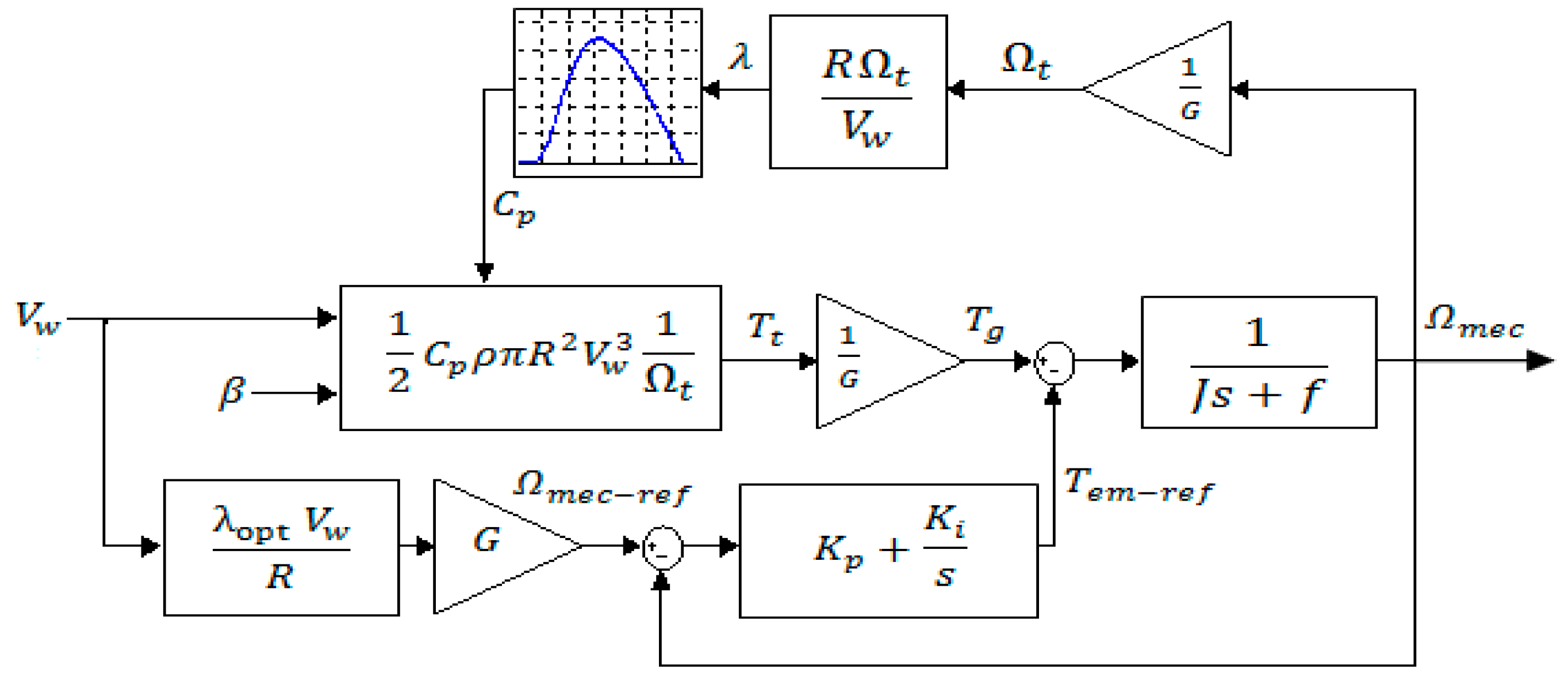
Figure 3.
Single-line diagram of a wind farm.
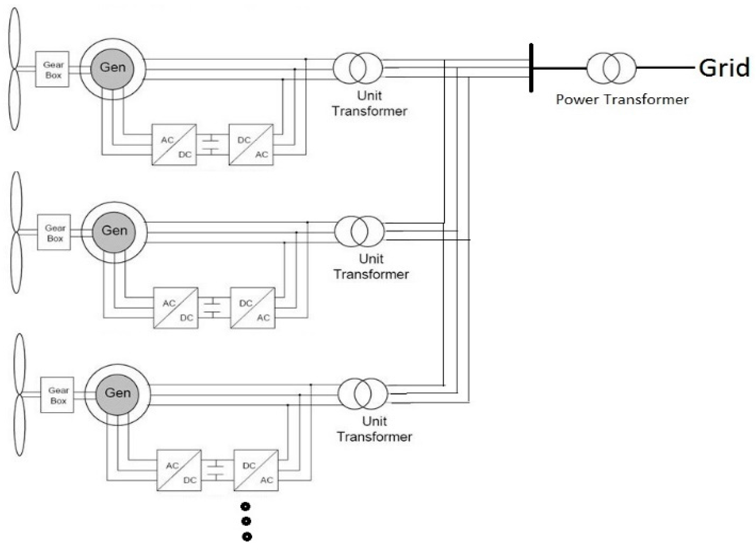
Figure 4.
P–δ and Q–δ curves.

Figure 5.
Single line diagram of the five-bus network with a wind farm.
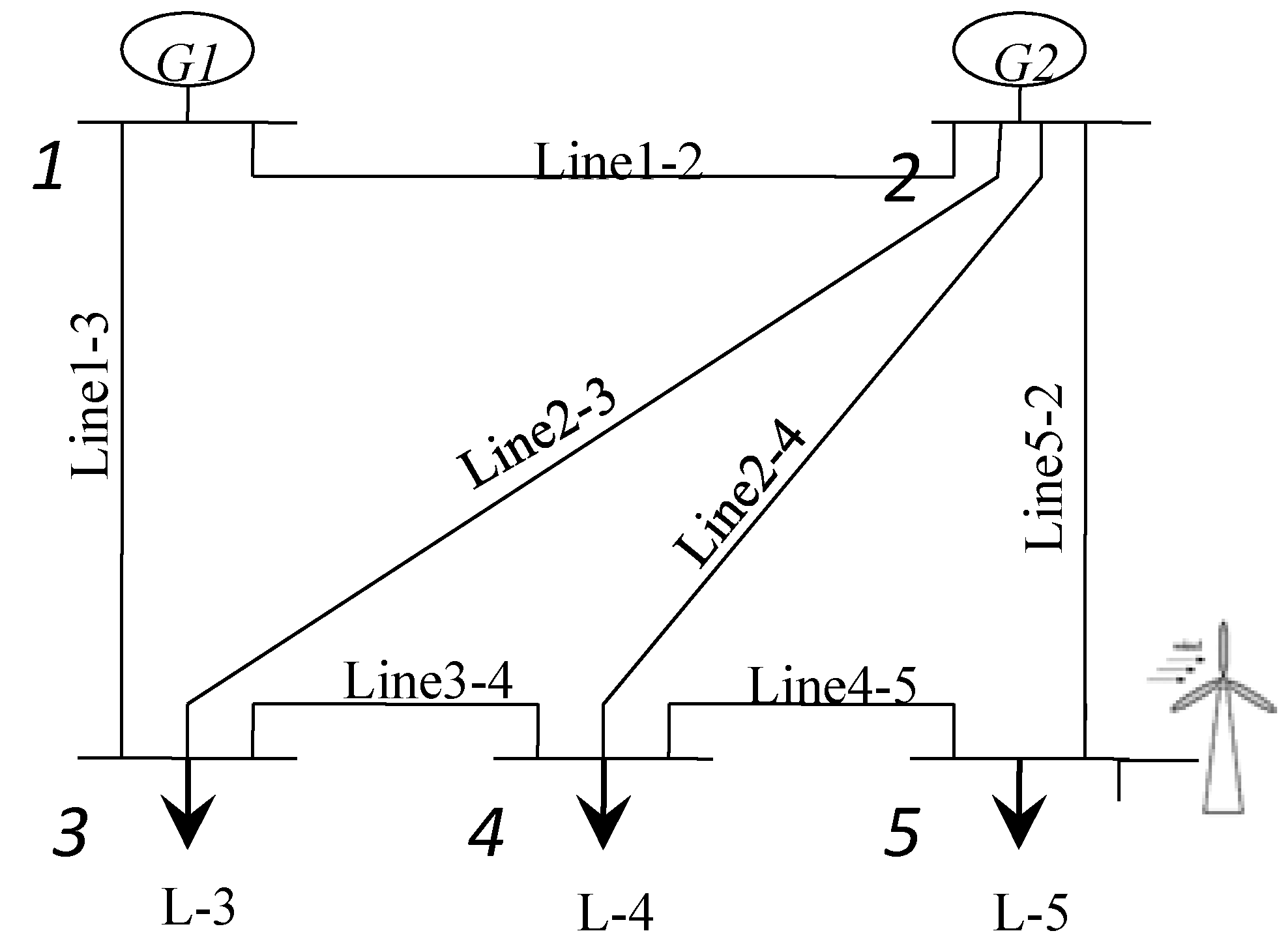
Figure 6.
Representative direct graph of the five-bus network.

Figure 7.
Yearly wind speed variation.
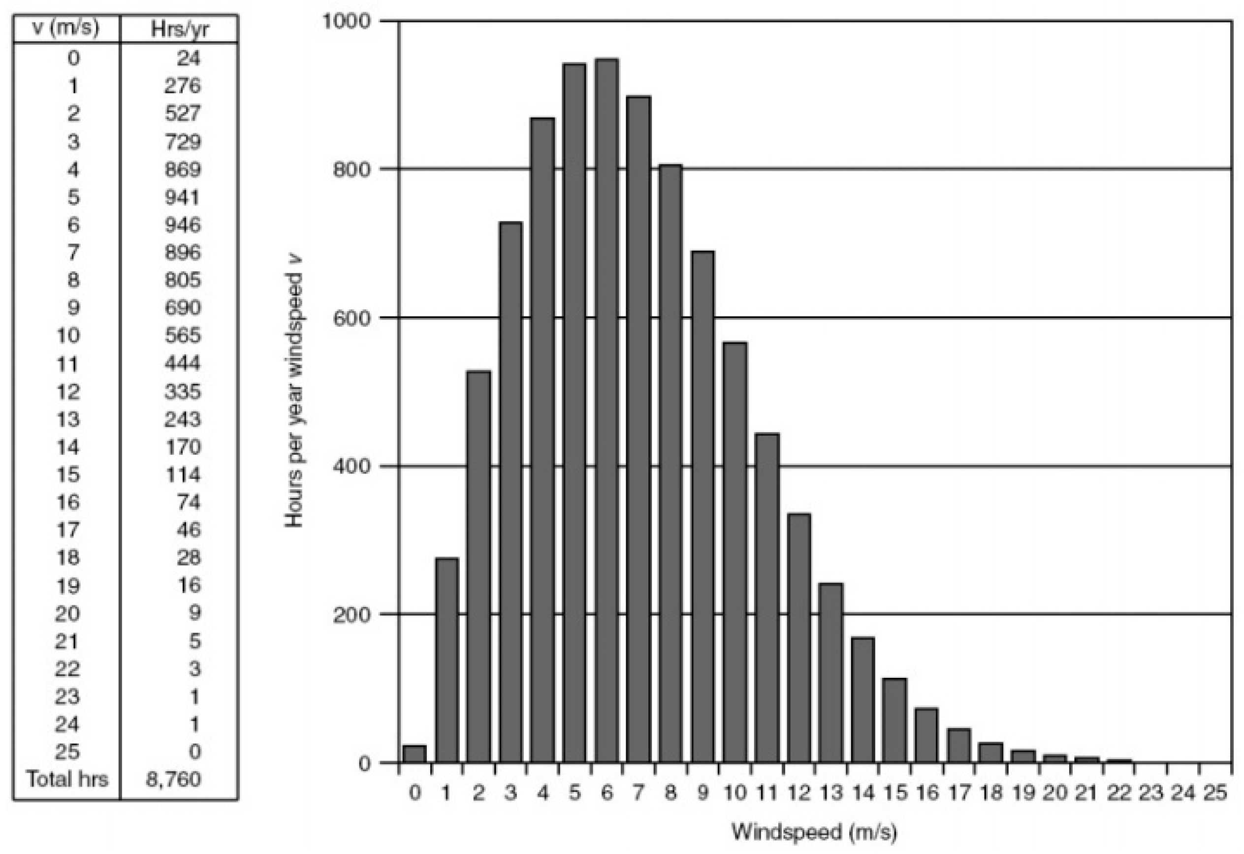
Figure 8.
Wind power output with steady wind speed.

Figure 9.
Bus losses with different wind farm locations.

Figure 10.
Active power flow on the lines before the integration of the wind farm.
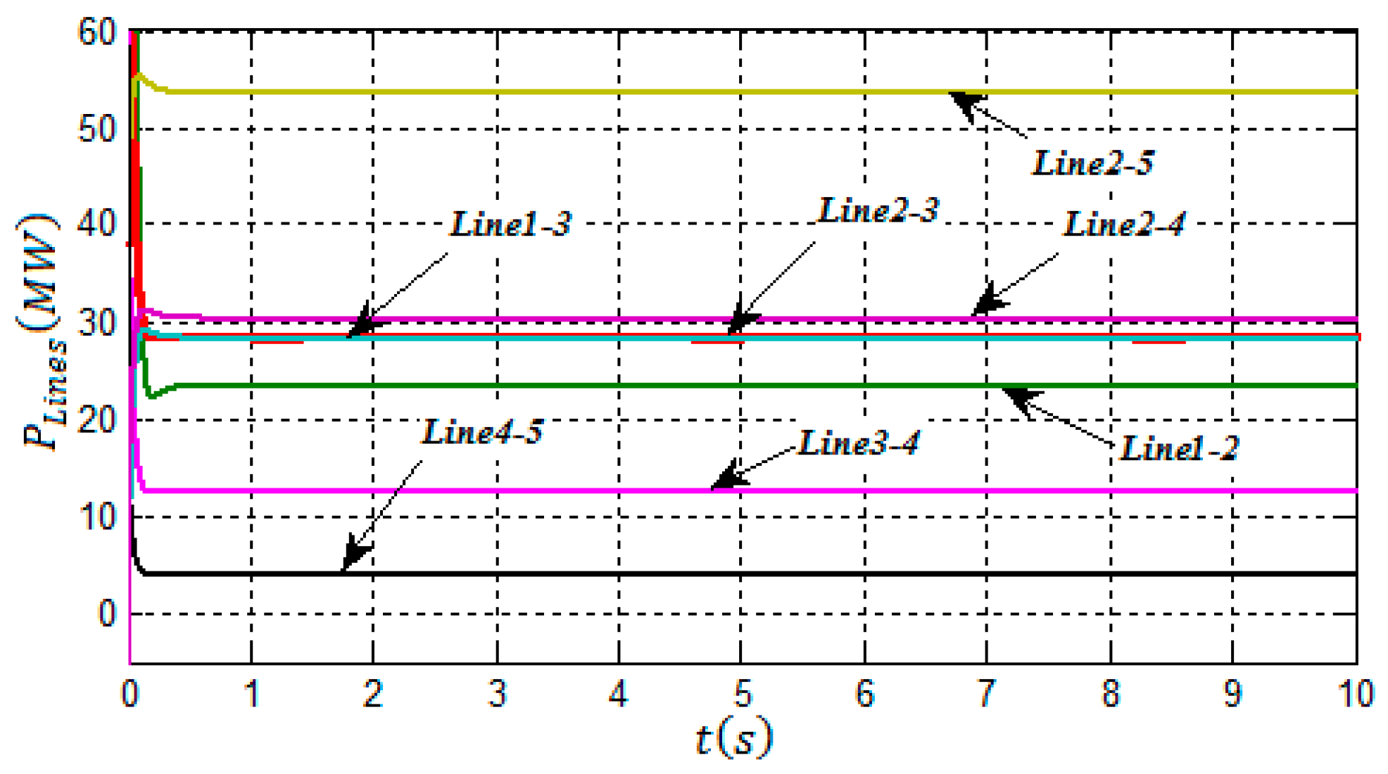
Figure 11.
Active power losses in the lines before the integration of the wind farm.

Figure 12.
Active power flow on the lines with the wind farm connected at bus 5.
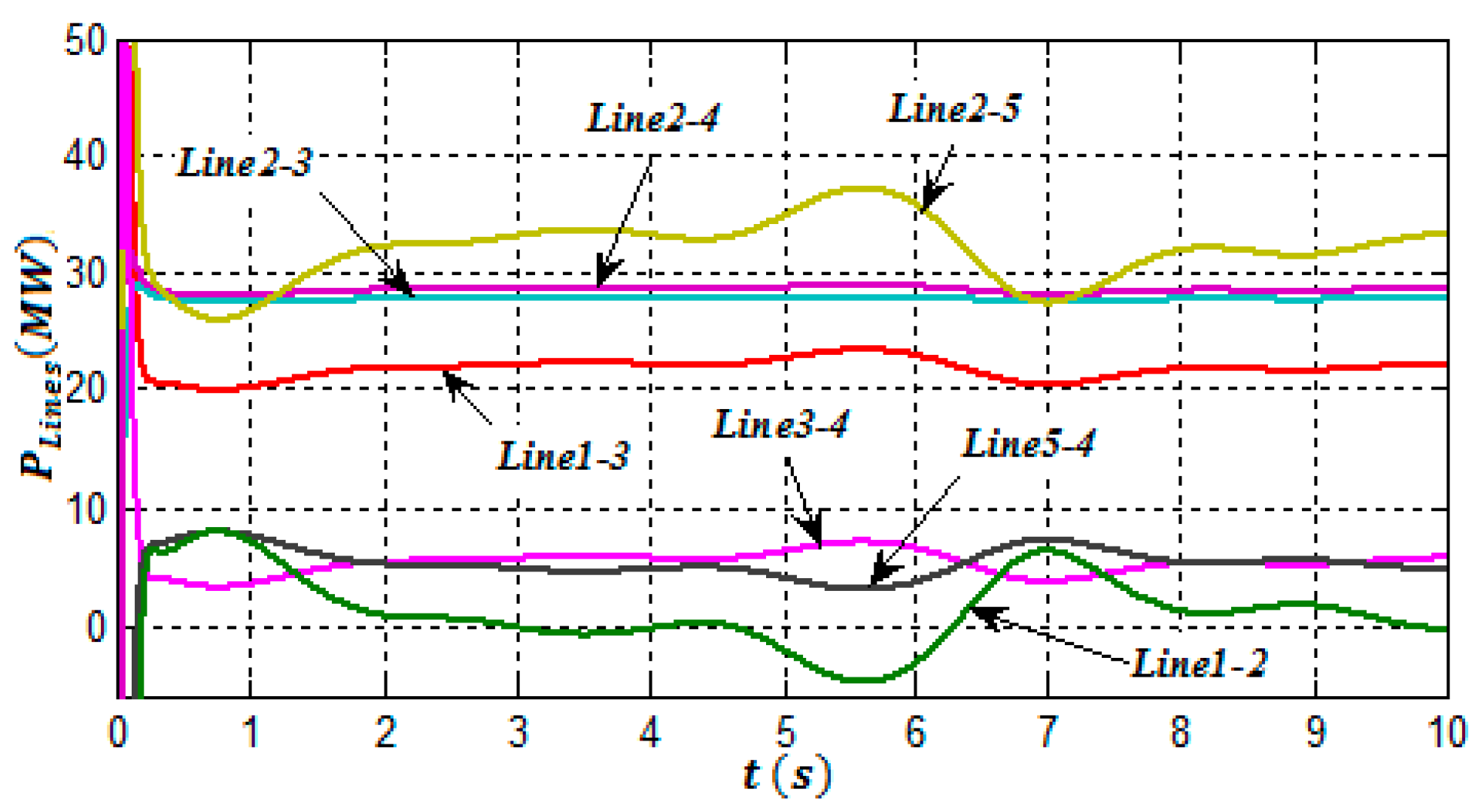
Figure 13.
Active power losses in the lines with the wind farm connected at bus 5.

Figure 14.
Active power losses in the network before and after integration of the wind farm.

Figure 15.
Comparison of annual average real power losses by the analytical method and Simulink.

Table 1.
Generation, load demand, and losses for the five-bus IEEE system.
| Unit | Total (MW) |
|---|---|
| Total Generation (PG1, PG2) | 148.05 |
| Total Demand (PD3, PD4, PD5) | 145 |
| Total real power loss | 3.05 |
Table 2.
Total real power losses for bus 5 with the wind farm.
| Wind Speed (m/s) | Hours Per Year | Power Output of Wind Farm (MW) | Total Real Losses (MW) |
|---|---|---|---|
| <3 or >25 | 827 | 0 | 3.05 |
| 3 | 729 | 0.9117 | 3.049 |
| 4 | 869 | 2.161 | 3.00 |
| 5 | 941 | 4.220 | 2.89 |
| 6 | 946 | 7.293 | 2.77 |
| 7 | 896 | 11.582 | 2.58 |
| 8 | 805 | 17.288 | 2.37 |
| 9 | 690 | 24.616 | 2.12 |
| 10 | 565 | 33.767 | 1.87 |
| ≥11 | 1489 | 44.944 | 1.66 |
| Annual average real power losses | 2.53 | ||
© 2017 by the authors. Licensee MDPI, Basel, Switzerland. This article is an open access article distributed under the terms and conditions of the Creative Commons Attribution (CC BY) license (http://creativecommons.org/licenses/by/4.0/).
Share and Cite
MDPI and ACS Style
Al Ameri, A.; Ounissa, A.; Nichita, C.; Djamal, A. Power Loss Analysis for Wind Power Grid Integration Based on Weibull Distribution. Energies 2017, 10, 463. https://doi.org/10.3390/en10040463
AMA Style
Al Ameri A, Ounissa A, Nichita C, Djamal A. Power Loss Analysis for Wind Power Grid Integration Based on Weibull Distribution. Energies. 2017; 10(4):463. https://doi.org/10.3390/en10040463
Chicago/Turabian StyleAl Ameri, Ahmed, Aouchenni Ounissa, Cristian Nichita, and Aouzellag Djamal. 2017. "Power Loss Analysis for Wind Power Grid Integration Based on Weibull Distribution" Energies 10, no. 4: 463. https://doi.org/10.3390/en10040463
Note that from the first issue of 2016, this journal uses article numbers instead of page numbers. See further details here.