
Risk-Based Dynamic Security Assessment for Power System Operation and Operational Planning
by
Emanuele Ciapessoni
1, 
Diego Cirio
1,
Stefano Massucco
2,*,
Andrea Morini
2, 
Andrea Pitto
1 and
Federico Silvestro
2 1
Ricerca sul Sistema Energetico—RSE S.p.A., Milan 20134, Italy
2
Department of Electrical, Electronics and Telecommunication Engineering and Naval Architecture, DITEN, University of Genova, Genoa 16145, Italy
*
Author to whom correspondence should be addressed.
Energies 2017, 10(4), 475; https://doi.org/10.3390/en10040475
Submission received: 23 January 2017
/
Revised: 9 March 2017
/
Accepted: 28 March 2017
/
Published: 1 April 2017
(This article belongs to the Special Issue Advances in Power System Operations and Planning)
Abstract
:Assessment of dynamic stability in a modern power system (PS) is becoming a stringent requirement both in operational planning and in on-line operation, due to the increasingly complex dynamics of a PS. Further, growing uncertainties in forecast state and in the response to disturbances suggests the adoption of risk-based approaches in Dynamic Security Assessment (DSA). The present paper describes a probabilistic risk-based DSA, which provides instability risk indicators by combining an innovative probabilistic hazard/vulnerability analysis with the assessment of contingency impacts via time domain simulation. The tool implementing the method can be applied to both current and forecast PS states, the latter characterized in terms of renewable and load forecast uncertainties, providing valuable results for operation and operational planning contexts. Some results from a real PS model are discussed.
1. Introduction
The increasing complexity of power system (PS) dynamics, due to the penetration of non-synchronously connected generation, make the assessment of instability phenomena a fundamental need in security analyses, both in real time operation and in operational planning. Moreover, the need to address multiple contingencies, potentially leading to widespread blackouts, suggests Transmission System Operators (TSOs) adopting risk-based approaches [1] to assess power system (PS) security.
Probabilistic risk-based approaches have been adopted for many decades in power system planning [2], but are relatively new in security assessment for operational context, where the N-1 criterion is still deemed to be a good tradeoff between completeness and computational time. Though several risk-based approaches to security assessment have been proposed by researchers in the last few years [3,4,5,6,7,8,9,10], the risk concept has been introduced only very recently by a few operational standards to deal with extreme events affecting an uncertain PS [11,12,13].
Many risk-based tools only deal with static impact of a contingency (in terms of post-contingency steady-state high currents or low voltages). Applying risk-based approaches to Dynamic Security Assessment (DSA) is more challenging because dynamic models are quite more complex to deal with (analysis techniques are less flexible and computation effort is higher); moreover, the outcome of a contingency does not only depend on the affected components and initial system state, but also on control and protection system parameters, as well as fault type, location, and clearing sequence. In [3], a transient stability margin from Potential Energy Boundary Surface (PEBS) theory is used to quantify the impact of a contingency on transient stability. Risk-based approaches are suitable to study the effects of uncertainties which affect both the system state (in operational planning studies) and the PS response to disturbances (major sources of uncertainties in on-line operation where the system state is “known” with good approximation). In particular, Intelligent Systems (IS) and fuzzy inference can be exploited in the context of dynamic security assessment under uncertainties for operational planning studies: reference [6] proposes an Artificial Neural Network (ANN) based method to quickly estimate the long-term voltage stability margin. In [7], the authors present an innovative IS based on Extreme Learning Machines, which learns very fast and provides an estimate to the credibility of its DSA results, allowing accurate and reliable results in pre-fault DSA analyses, thus avoiding long time-domain simulations in online sessions. In [8], a hierarchical IS, the ensemble learning strategy based on Neural Nets with random weights, is proposed to analyze short term voltage stability. In [9], a Monte Carlo method is used to get the pdf’s of small and large disturbance rotor angle stability indicators, considering load and generation and fault-specific uncertainties; the pdf’s are subsequently decomposed into regions based on user-defined thresholds and the outputs of this decomposition are analyzed using a fuzzy inference system to complete a stability assessment. In [10], a very large amount of dynamic simulations are performed to train Decision Trees and generate security rules which are then used for security assessment for on-line operation.
This paper presents the innovative Risk-Based Dynamic Security Assessment (RB-DSA) approach developed within the EU FP7 Project AFTER (A Framework for electrical power sysTems vulnerability identification, dEfense and Restoration). The aim of RB-DSA is to quantify the risk of instability phenomena in the system due to a set of critical, single, and multiple (also dependent) contingencies selected on the basis of the threat scenarios affecting a given current (or forecast) operating point. Thus, the RB-DSA represents an important step forward with respect to more conventional risk-based approach, such as [3], because the proposed methodology does not compute the failure probabilities from historical records but from short-term forecasts of hazards and from vulnerability curves of components, thus linking Hazard Analysis to Contingency Planning, which up to now have been considered as separate “problems”. This is also an added value with respect to IS systems: In fact, the IS training set is built starting from a plausible PS states elaborated on the basis of historical data, which does not assure the good performance of such tools in case of inadvertent “new” states occurring in the future.
The paper is organized as follows: Section 2 illustrates the risk-based dynamic security assessment tool developed in the AFTER project. Section 3 presents the indicators used to quantify the impact and risk of contingencies on a power system. Section 4 describes the test system under study and discusses some simulation results. Section 5 concludes the paper.
2. The AFTER Risk-Based Dynamic Security Assessment Framework
The fundamentals of the AFTER methodology and tool are presented in [14]. Following a brief overview of the AFTER risk assessment framework, the section presents the main features of the developed RB-DSA methodology and tool. The tool can be applied to a forecast (uncertain) or a specific (current or known) PS state, thus focusing on both operation and operational planning applications.
2.1. AFTER Methodology and Tool
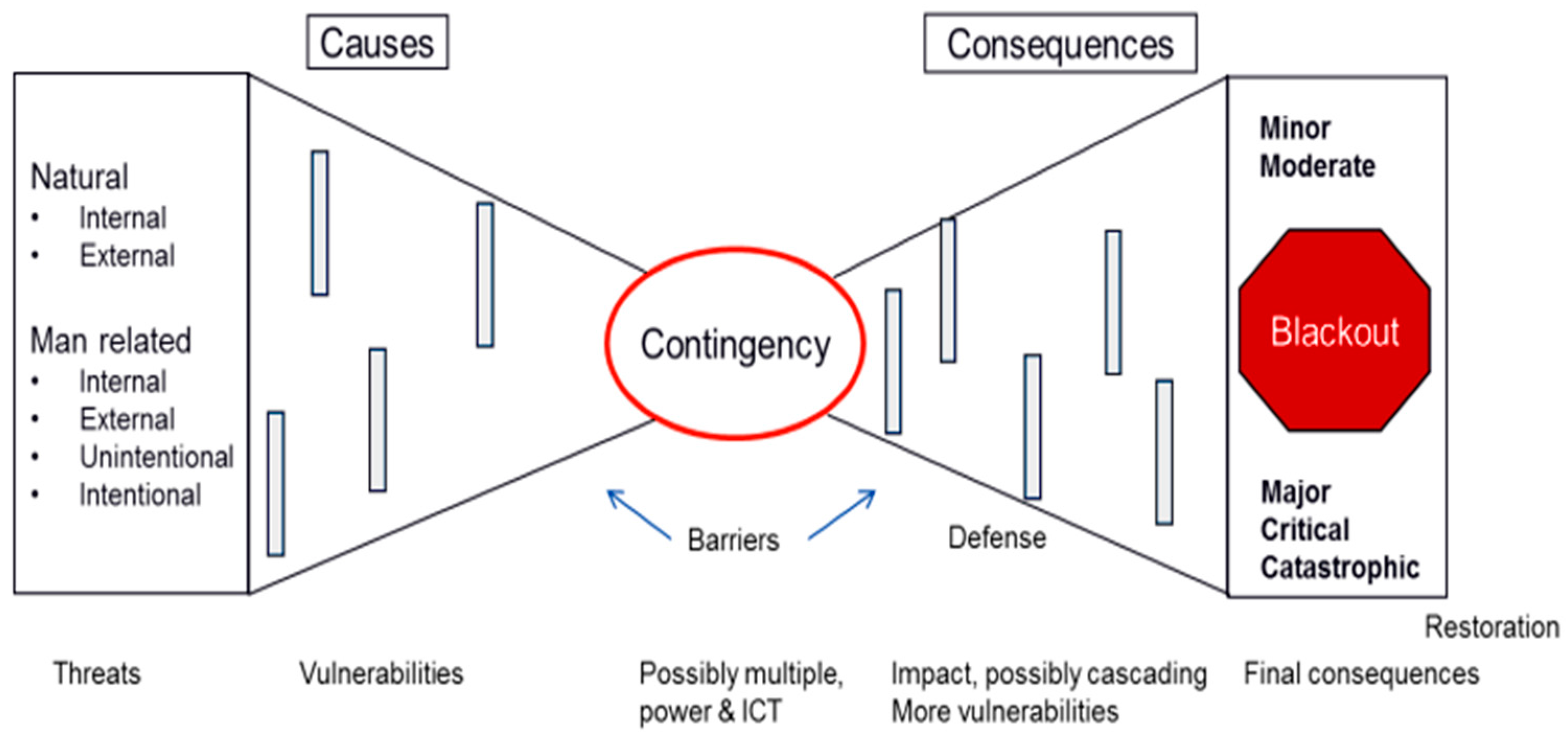
The probabilistic risk assessment methodology developed within AFTER [15,16] is based on the conceptual bow-tie model describing the relations between causes and consequences of unwanted events. Figure 1 shows an example where the main unwanted events are contingencies potentially leading to cascading and blackouts, i.e., with severe (major, critical, or catastrophic) consequences.
The left side shows the adopted threat classification, which distinguishes natural from man-related threats, both of them are classified as internal or external to the power system: the man-related ones are further divided into intentional (sabotage, etc.) or unintentional (human error). Threats may lead to a contingency through a set of causes exploiting vulnerabilities, while the contingency may lead to different consequences (impacts) through a set of circumstances. The initial impact may in turn affect other vulnerabilities, incepting a cascading process that finally results in a blackout. The hazard analysis performed in the AFTER framework provides a coherent framework where different hazards (each one usually managed with its own “ad hoc” models and assumptions) are modelled via a unique mathematical formulation. Moreover, its outcomes are the inputs for the next modules aimed at assessing the power system security, thus reproducing the straightforward causal process from hazards to disturbances. Figure 2 shows the architecture of the prototype, developed in MATLAB environment and aimed to power and Information Communication Technology (ICT) risk assessment.
In the proposed modeling framework, a threat can affect different vulnerabilities of power-ICT components by activating stress variables (i.e., the physical quantities through which the threat affects the component vulnerabilities). For example, a tornado induces additional mechanical forces to transmission line pylons; the stress may in turn cause the failure of a component.
Vulnerability can be mathematically interpreted as the conditional probability of failure of a component given the occurrence of a specific threat. In turn, any threat can also be described in probabilistic terms; e.g., the probability of a natural threat, such as lightning or a fire, depends on the weather or environmental conditions at the time of the event.
Based on the above, the computation of component failure probability is performed making use of threat and vulnerability probabilistic models. In module F (Figure 2), all components are ranked based on their failure probability PF. The “critical components”, defined as the ones “explaining” the largest fraction of total failure probability, are identified. To this aim a cumulative sum screening technique [17] is used, which works as follows:
- Rank failure probability of all components into decreasing order, creating a map C(l) = l′ between l and l′ (indexes of original and ordered components) s.t. .
- Calculate the cumulative sum for each ordered component with index l′ .
- Find line lTOT whose F minimizes where α, the coefficient of the sum of failure probabilities of all components, is called “fraction of explained total failure probability”.
- Get minimum failure probability threshold PFTOT as: .
- Select components with failure probability higher than PFTOT.
The generic “contingency” at the system level consists of the failure of one or more components. Starting from critical components, an enumeration technique is adopted in module C to generate a large set of single and multiple (also common mode and dependent) contingencies, including busbar or half-busbar faults, power plant outages, and double circuit outages. In a preliminary screening phase the risk associated to each contingency is computed by combining contingency probability with a fast evaluation of the impact, based on topological or DC load flow-based metrics. Only those contingencies which show a risk value higher than a minimum risk threshold are analyzed in detail by both power flow based analyses and dynamic simulations run in module R: the results of these analyses are synthetized in impact indices in module I.
The final outcome consists of impact-based and risk-based ranking lists of contingencies. In case of a forecast PS state, the tool provides the Complementary Cumulative Distribution Curves (CCDFs) of the risk indicators. In particular, the RB-DSA tool evaluates the severity of the contingency with respect to angle voltage and frequency dynamics by calculating dynamic impact indicators and combining them with contingency probability.
2.2. Failure Probability Assessment: Validation and Data Availability
The characterization of the probabilistic models is one of the main barriers for the application of probabilistic techniques in real world power system operation. In this regard, reference [16] collects references which provide guidelines for statistical analyses of historical data and for the development of probabilistic models related to different threats and vulnerabilities (from transmission equipment to distribution networks), with special focus on long/medium term horizons. Instead, short term models of threats, like the ones modeled in the present paper, are tuned considering measurements of stress variables (e.g., wind speed, precipitation rate, etc.), available from technical disturbance reports concerning specific “real life” weather/environmental hazards.
Some interesting results have been derived from benchmarking the threat and vulnerability probabilistic models relevant to lightning against real world data. As an example, from statistical analysis of real data [18], the yearly average failure rate of a 220 kV transmission line for the Italian system is 3.5 × 10⁻¹⁰ failures/(km·s). Assuming 15 h of severe storms, in the region under study, allows for estimation of the failure rate over “bad weather” quarters of an hour:
This means 5.4 × 10⁻⁵ failures/(quarter of hour) for any span of a line (assuming a 300 m long span for a 220 kV line). The simulation of a severe lightning storm was performed by the AFTER tool on a realistic 220 kV test grid, assuming a flash-to-ground density of 3.2 flashes/(h·km2), i.e., a realistic value for severe storms as in [17]. Results shows that the maximum 10 min failure probability over the most exposed 300 m long span of a 220 kV line is 3.6 × 10⁻⁵ failures/(10 min), in good accordance with estimates from historical data.
2.3. Contingency Definition in Dynamics
In dynamic simulations, a contingency is characterized by more elements than in load flow-based analyses. In fact, besides the components that are in outage and the PS state, the features which affect the dynamic response are:
- Specific parameters of the fault (location, type, duration).
- Control, protection, and defense systems (which affect the behavior over fault-on and post-fault periods).
With regard to point 1, the proposed RB-DSA exploits the probabilistic models of component vulnerabilities and of the threats affecting the current (or forecasted) system state, to perform a probability-based filtering of the most critical components: this drives the choice of the contingency generation, thus, the location of the faults to be investigated by the RB-DSA. The simulations herein presented only consider three-phase faults but this is not a limitation for the tool which can simulate any type of symmetric and a-symmetric faults.
As for point 2, the severity is mainly determined by the behavior of control and protection systems in the fault-on and post-fault periods. This aspect is not thoroughly tackled by other risk-based DSA approaches [3]. The clearing time depends on the typical TSO settings of primary and back-up protections [19]. In particular, Table 1 reports the different types of busbar and branch contingencies which differ for the behavior of primary and back-up protections in clearing the fault. The time domain simulator evaluates the system dynamic response in the first seconds after each contingency, including primary and back up protection logics, i.e., the Bus Differential Protection (BDP), distance relays (zones 1 and 2), overcurrent protection for transformers, and breaker failure device [19].
The failure probabilities of involved components (ptr2, pl and psb respectively for transformers, lines and busbars) are calculated from hazard/vulnerability analysis, while the “fail on command” probabilities (pCBj, p_bdpj, p_dsj, p_ptj and p_BDP respectively for Circuit Breaker (CB), BDP signal, distance protection signal, transformer protection signal to component j, and BDP operation) are retrieved from literature [20]. K stands for bus coupler.
3. Contingency Impact and Risk Assessment
The impact of each of the contingencies is evaluated in terms of three dynamic severity indexes, respectively related to angle, over- and under-voltage, and frequency instabilities. Impact indicators are based on rotor angle, bus voltage, or mean frequency deviations. Dynamic risk indexes are defined as the expected value of the contingency impact and are calculated by combining contingency probability and impact. Risk and impact indicators can be used to rank contingencies, to focus operators’ attention on those events which may jeopardize the PS stability in the operating point under analysis.
3.1. Transient Stability Impact
Angle impact indicators consist in integral metrics measuring the “cumulated” displacements, over time, between rotor angles and center of inertia angle weighted on generator inertia constants: machine angles are obtained by the time domain simulator. In particular, the Integral Squared Generator Angle (ISGA) [21] indicator is adopted:
where is the i-th machine rotor angle, is the Center Of Angles (COA), Mi = 2 × Hi with Hi = the i-th machine inertia constant on the system base, and , Ng is the number of generators belonging to the same electrical island. T is the time window (s) and t0 is the initial time instant.
3.2. Voltage Stability Impact
Voltage impact indicators consist of integral metrics measuring the “cumulated” displacements, over time, between node voltages and maximum/minimum voltage security limits weighted on node nominal voltages: voltages are obtained by the time domain simulator. The adopted Dynamic Under Voltage (DUV) and Dynamic Over Voltage (DOV) indexes are shown in Equation (2) and represents the mean under- and over-voltage deviations over a time window T starting from time instant t0 [22].
where are respectively the voltage, the maximum threshold and the minimum threshold for h-th node. A reasonable range for can be given by the typical settings used by TSOs for under-voltage load shedding activation (0.85–0.89 p.u.). is set considering the upper limits of voltage operational range for motors and generators (1.15–1.20 p.u.).
3.3. Frequency Stability Impact
System frequency can be evaluated as the weighted average of machine angles in the same electrical island, where weights are the inertia constants on the system base. However, the presence of transients due to faults can alter the assessment of the slower frequency dynamics of interest. To filter out these transients, the RB-DSA calculates a moving average on a 500 ms window of the two signals: frequency f and frequency time derivative df/dt. The results are the mean average and the Rate of Change of Frequency (ROCOF). The severity frequency indicators are defined as follows [23]:
where deadbf, DFDOWN and DFUP are respectively the mean frequency sensitivity band, the max admissible under-frequency and over-frequency deviation according to TSO standards, while min ROCOF, ROCOFDOWN and ROCOFUP are respectively the ROCOF sensitivity band, the max admissible downward and upward ROCOF deviation.
3.4. Risk Indicators
In general terms, risk is defined by the set of possible events (“contingencies”), their probability of occurrence, and their impact on the system. More specifically, risk is quantified as the expected values of the impact of a contingency (or a set of contingencies). With such a definition, contingency risk indicators are simply calculated by multiplying the impact indicators with contingency probabilities found in Subsection II.B. Risk indicators may refer to a set of contingencies deemed as dangerous under specific weather/environmental conditions (total risk indicators) or to one contingency (individual risk indicators): The former indexes measures the overall risk of the PS exposure to dynamic instabilities, the latter ones are useful to rank contingencies and focus operators’ attention on the most risky events.
3.5. Assessing the Effect of Uncertaintites on Forecast PS State
At the operational planning stage, the RB-DSA can be used to assess dynamic risk over a “forecast” operating point, given k-hour ahead renewable and load forecasts. In particular, the goal is to answer the following question: How does the operational risk of a PS subjected to a set of contingencies depend on the forecast error distributions of Renewable Energy Sources (RES) production and load absorptions available k hours ahead?
To this aim, the RB-DSA exploits the Point Estimate Method (PEM) and Third Order Polynomial Normal Transformation (TPNT) to generate a set of PS states starting from the marginal probability distributions of the stochastic INPUTS (k-hour ahead forecast errors of the RES injections and load absorptions) and their correlation. Then, the RB-DSA runs impact and risk assessment on each of the abovementioned states. The results consist of probability distributions of dynamic risk indicators (on the whole contingency set and/or for each contingency) and provide alarms in case of a too high probability that exceeds max risk limits.
In the present models, the standard deviation of RES generation forecast errors depends on the level of aggregation and geographic extension of RES, and by the forecast horizon under investigation. The standard deviation associated with load forecasts is usually very low (typically 1–4% of the rated power). In general, the k-hour ahead forecast error distributions for RES (solar and wind plants) can be derived from climatological models or from more advanced models like ensemble forecasts. The non-symmetry of the RES forecast errors, derived from statistical analyses of historical data, suggests the use of non-symmetric distributions (like beta distributions), see also [24].
Dependence among inputs is tackled using the Third Order Polynomial normal transformation. More details about this technique can be found in Appendix A.
3.6. RB-DSA Outcomes
The typical outcomes of the RB-DSA tool consists of:
- Risk and impact based ranking lists of contingencies, to focus operators’ attention and let them deploy suitable corrective actions, for on-line operation applications.
- Complementary Cumulative Distribution Functions (CCDF), i.e., the probability of overcoming a certain x-value) for risk and impact indicators referred to the whole threat scenario (global indicators) or to each contingency (individual indicators), useful for operational planners.
The accuracy of the RB-DSA results essentially depend on the accuracy of (1) contingency probability, (2) the system response to the contingencies, and (3) the uncertainties on the PS state. Section 2.2 has demonstrated the good match between short-term single outage probabilities with real-world available data for a “lightning” threat. Standard impact indicators already proposed and validated in literature are used to quantify the impact of contingencies. As far as item (3) is concerned, the PEM method combined with TPNT transformation (used to model uncertainties on PS state) has been validated by the authors against the Monte Carlo method in [24], demonstrating a good match between the probability densities of risk indicators evaluated by the two methods.
4. Test System and Simulation Results
This section presents the results of the RB-DSA application on a model of a realistic 220/400 kV system.
4.1. Test System and Simulation cases
The test system represents a portion of the Italian Extra High Voltage (EHV) grid in a high load operating condition (autumn peak load) in the early 2000s. The power system includes 80 lines, 70 electrical nodes, and 20 generators. The dynamic model of the test grid includes the 6th order model of synchronous machines, their prime movers with governors, and their automatic voltage controls and exciters. As RES are usually interfaced with the bulk systems through power electronics, the displacement of much of the power from conventional units to renewables determines a lower system inertia, which affects both angle stability and frequency stability. Moreover, voltage stability properties can change as a result of the voltage controls enabled by converters (especially those with Voltage Source Converter (VSC) technology). The time-domain simulator allows for representation of the RES with different levels of detail: from a simple injection with constant P (active power) and Q (reactive power), to a more refined VSC model including the inner (current) and outer control loops of the typical Park’s transformation based controller [25]. In both cases, the dynamics of the specific RES “behind” the VSC is neglected, which can be a reasonable assumption due to the brevity (a few seconds) of the time interval for simulations.
The abovementioned operating state represents the “current” system state for the simulation cases describing the RB-DSA applications to on-line operation sessions. In this context uncertainties only concern the occurrence of contingencies over a future short time interval (10–15 min).
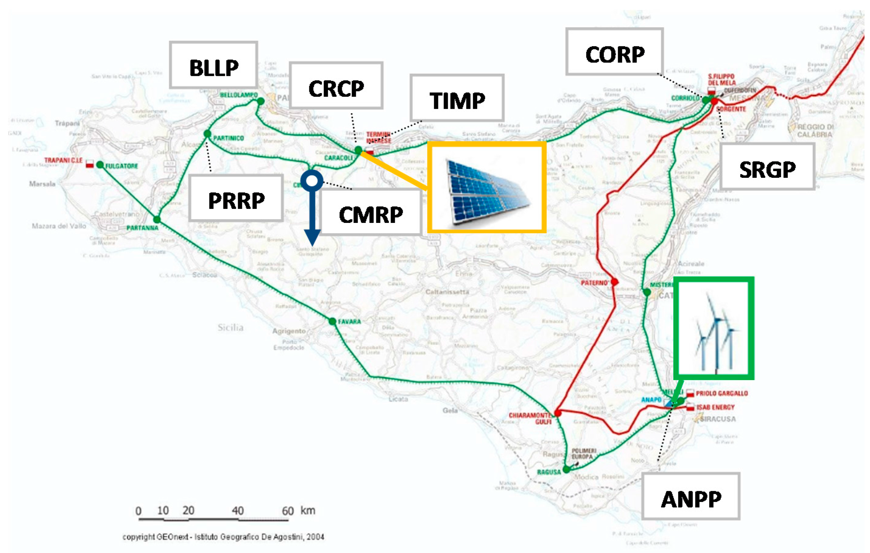
In operational planning applications of the RB-DSA, the available operating state is the “forecast” state available k hours ahead and subjected to RES and load forecast uncertainties. To simulate these uncertainties in the presented simulations, some changes have been performed on the system: two hydro units at the ANPP power plant and one thermal unit at the TIMP power plant have been respectively replaced with two aggregated wind farm injections and one equivalent solar power injection with the same ratings. Moreover, a stochastic load is modeled at one 150 kV busbar of the CMRP substation. “ANPP”, “TIMP” and “CMRP” are few examples of identification code for the grid substations. Figure 3 shows the RES and stochastic load connection points to the grid and the identification codes for the substations mentioned in the analyses.
The resulting difference between the generators’ injections and the load absorptions is balanced by the “slack” unit at the SRGP substation which represents the behavior of continental units. The forecast errors of the aggregated RES injections are modelled as a beta distribution, where mean and variance are calculated from the data reported in Table 2.
The load forecast error is modelled as a normal variable with a mean and a standard deviation of 0.9% and 3%, respectively, of the rated power (corresponding to typical values for an autumn peak hour condition). The contingency set that is under study includes the set of single and multiple (also dependent) contingencies which are selected as “dangerous” by the AFTER risk assessment tool, for a mild wind storm affecting the West side of the island. Different simulations have been performed: two of them, discussed in detail, are reported in Table 3.
4.2. RB-DSA Application for On-Line Operation
The following section intends to demonstrate an application of the RB-DSA tool in operation. For this purpose, we assume that RES generation is known with good accuracy, we are given the known system “state”, the tool analyses the dynamic response of the PS to a set of single and multiple dependent contingencies, which are more risky for the specific threat scenario under study. Telepiloting among distance relays is assumed out of service, thus the zone 2 delay is 400 ms.
Table 4 shows the top 20 list of ranked contingencies based on the angle stability risk index.
It can be noticed that after N-1 branch outages, two N-k contingencies affecting the CMRP substation have the largest contributions to the risk, mainly due to their significant probability of occurrence. Subsequent contingencies are N-2 dependent contingencies (double circuit failures) and some N-k dependent contingencies with high impacts (higher than 1), which involve both power component failures and ICT malfunctions, and which determine the loss of synchronism of some units in the system (this is checked with conventional criteria—e.g., maximum angular deviations—in time domain simulations). The results demonstrate the importance to also consider N-k dependent contingencies which are neglected in “conventional” dynamic security assessment analyses; these usually only consider contingencies selected according to a “credibility” (e.g., the N-1) criterion. In particular, the probability of occurrence of some N-k contingencies caused by a severe hazard may be relatively high compared to the outage of a single component (N-1) located far from the impact area of the hazard. This underlines the added value of the proposed RB-DSA method with respect to similar risk based approaches. In fact, the AFTER approach can exploit the forecasts of an incumbent hazard and of the PS state to compute the short-term component failure probability (thus, also the contingency probability), which are of paramount importance in operation.
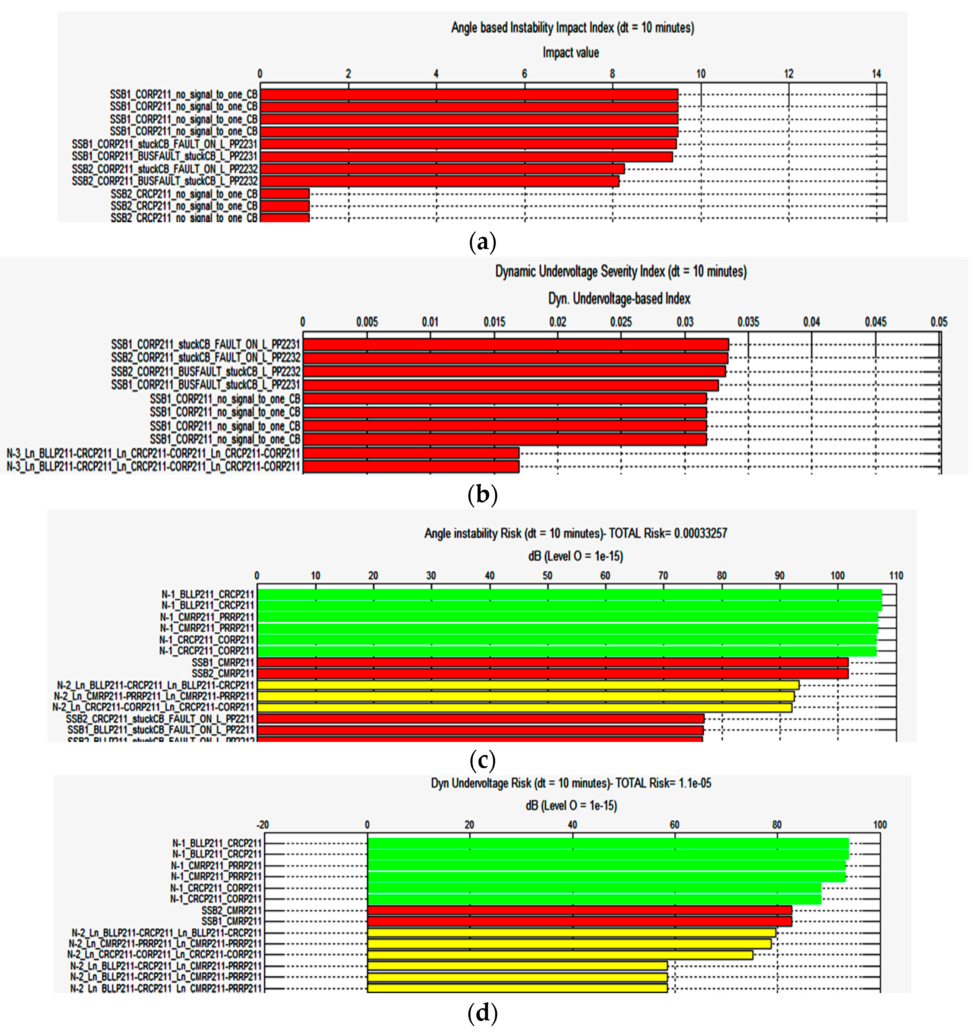
Figure 4 reports the impact and risk-based ranking lists for angle stability and dynamic undervoltages. Red, yellow, and green bars correspond respectively to N-k, N-2 and N-1 contingencies.
It can be noticed that for angle stability problems, the highest impacts are related to multiple N-k busbar contingencies, especially close to power plants (e.g., CORP and CRCP substations).
Due to telepiloting malfunction, high impacts both on angle and voltage transients are detected for those N-k contingencies which imply the intervention of back-up protections (like zone 2 for distance protections).
In particular, the application of a standard stability criterion (Maximum Angular Deviation) in time domain simulations shows that the ISGA transient stability impact metrics allows a clear separation between “stable cases” (impacts < 0.2) and “unstable cases” (impacts > 1).
4.3. RB-DSA Application to Forecast PS State
This section illustrates an example of application of the proposed RB-DSA over a forecast power system state affected by the uncertainties due to the probability distributions of forecast errors related to RES and loads, and available k-hours ahead of the PS state under study.
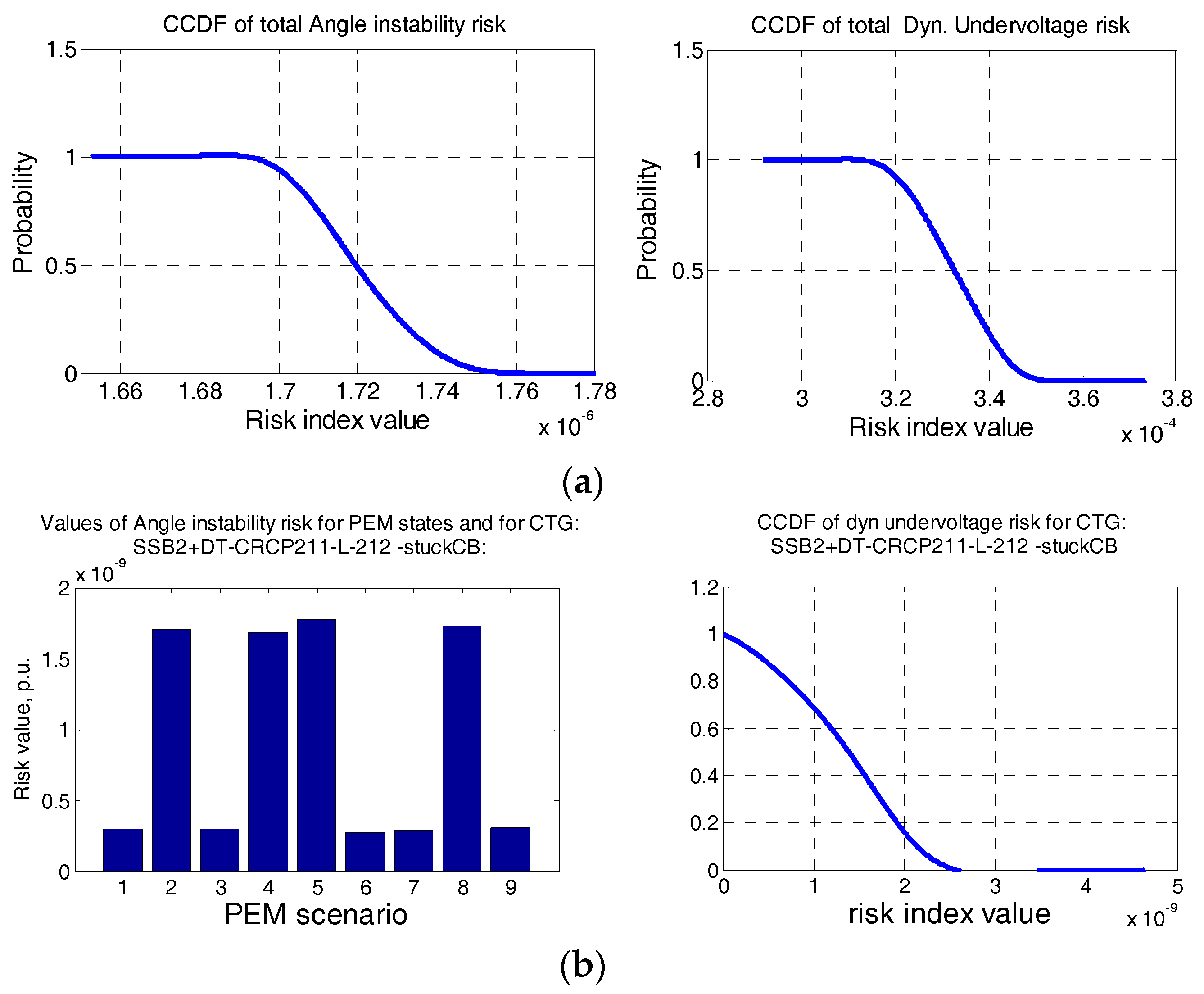
Figure 5 illustrates the CCDF of angle instability risk and of dynamic undervoltage risk indexes relevant to the whole set of contingencies (total risk) and to a specific contingency, which represents a fault on one of the lines of the double circuit between the CRCP and the BLLP substations, with one stuck breaker and the loss of all the bays connected to the half-busbar relevant to the stuck CB.
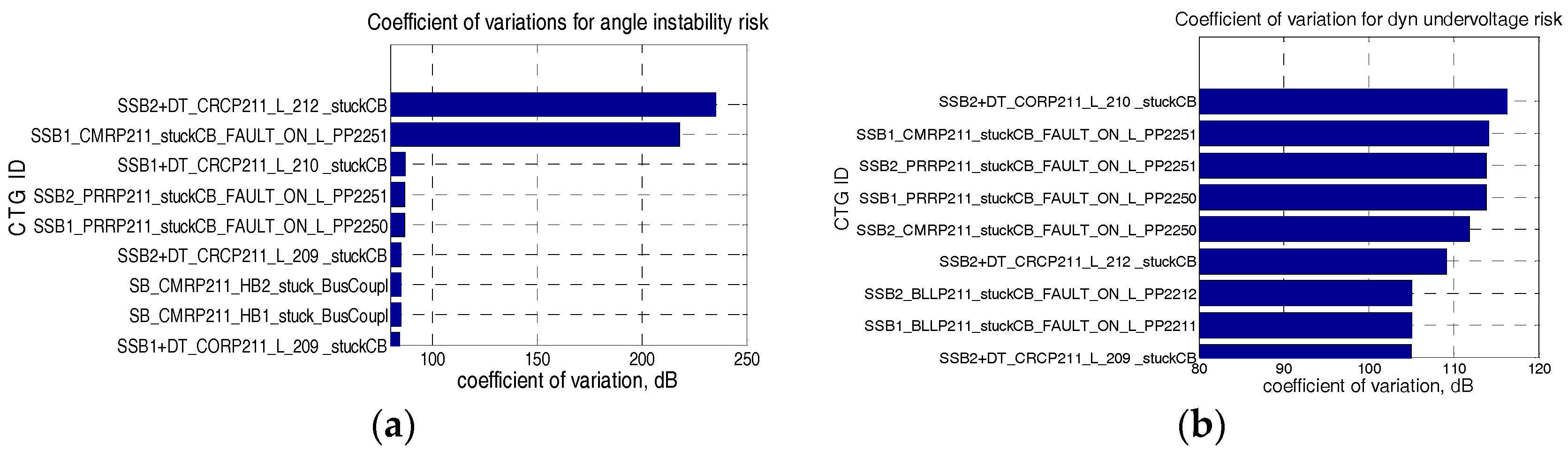
In the present case, forecast uncertainties do not significantly affect the total risk index which shows a small variance, due to the fact that the impact of N-1 and dependent N-2 contingencies (which mainly contribute to the total index) are little affected by the variability of the stochastic injections. On the contrary, the severity of a very impacting contingency “SSB2+DT_CRCP211_L212-stuck CB” can be greatly affected by the amounts of renewables: for some states analyzed by the PEM, the RES, and load configurations determine the rotor angle instability (angle severity impact largely greater than 1), while for other states, the system is stable (angle severity impacts much lower than 1). This is explained by the large difference in risk index values among the PEM states illustrated in Figure 5b, this instability is due to the loss of synchronism of a generating unit in the TIMP power plant, to which the equivalent solar farm injection is assumed to be connected. A large amount of RES increases the power flow between TIMP PP and the rest of the grid, and this can favour the angle instability of the conventional units of the same plant in case of persisting faults in the surrounding substations. The tool allows to quantify the effect of system state uncertainties on each contingency. With reference to angle and dynamic undervoltage problems, Figure 6 reports the coefficients of variation (CV) in dB, defined as , with μ and σ respectively mean and standard deviation of the individual risk index CCDF, and used to identify the contingencies whose risk is most affected by uncertainties (adopted base = 10−5).
The most affected contingencies which consist of two busbar N-k contingencies involving the loss of two double circuits: the former connects the BLLP substation in a heavy load area and the CRCP substation, and the other represents a heavily loaded path from East (generation area) to West (load area) on the 220 kV ring of the system.
5. Conclusions
This paper has proposed a risk-based dynamic security assessment method which can account for uncertainties affecting a power system state, initiating events (contingencies), and system response to contingencies themselves. In quasi real time operation, the tool can rank the selected contingencies on the basis of the threats currently affecting the system state, thus evaluating the risk of instability to which the PS is exposed, due to the contingencies. This can help operators focus on the most risky events, including multiple dependent contingencies on substation busbars and power plants. In operational planning, the tool can quantify the effect of uncertainties due to RES and load forecast errors on the risk of losing angle, voltage, and frequency stability, while looking at the complementary cumulative distribution functions of the risk indicators, and highlighting which disturbances show the highest impact sensitivity to these uncertainties. This information can be very valuable at an operational planning stage. Further works will focus on algorithms to elaborate optimal corrective/preventive control actions in order to reduce risk.
Acknowledgments
This work has been financed by the Research Fund for the Italian Electrical System under the Contract Agreement between RSE S.p.A. and the Ministry of Economic Development—General Directorate for Nuclear Energy, Renewable Energy and Energy Efficiency in compliance with the Decree of 8 March 2006.
Author Contributions
All the authors have worked on all the subjects (methodology, modeling, grid model preparation, SW implementation, simulation running, results discussion and paper writing).
Conflicts of Interest
The authors declare no conflict of interest.
Nomenclature
| Acronym | Meaning |
| ANN | Artificial Neural Network |
| BDP | Bus Differential Protection |
| CB | Circuit Breaker |
| CCDF | Complementary Cumulative Distribution Function |
| COA | Center Of Angles |
| DSA | Dynamic Security Assessment |
| DOV | Dynamic OverVoltage |
| DUV | Dynamic UnderVoltage |
| IS | Intelligent Systems |
| ISGA | Integral Squared Generator Angle |
| PEM | Point Estimate Method |
| PS | Power System |
| RB-DSA | Risk Based - Dynamic Security Assessment |
| RES | Renewable Energy Sources |
| ROCOF | Rate Of Change Of Frequency |
| TPNT | Third order Polynomial Normal Transformation |
| TSO | Transmission System Operator |
Appendix A. Third Order Polynomial Normal Transformation
The Third Order Polynomial Normal Transformation (TPNT) transformation permits one to extend the potentialities of probabilistic load flow based on Point Estimation Method (PEM) scheme also to dependent non-normal distributions. Given the marginal distributions FX of inputs X, the rationale is to express non normal variables X (i = 1, …, m) as a third order polynomial of dependent normal variables Z:
L-moments are calculated as a function of the expectation value of an order statistic EX [26]:
where with F and f are respectively the cumulative distribution function and the probability density function of stochastic variable X.
Also, Z variables are dependent and relevant correlation matrix ρZ can be derived from ρX by solving the equation below for any pair of X variables:
where are respectively the standard deviation and the mean value of variable i. Again, ρZ is positive definite and it can undergo Cholesky decomposition. GZ is the resulting matrix so that . Using matrix GZ it is possible to link transformed normal dependent variables Z to independent normal variable Y to which the PEM can be applied. The linear transformation between Z and Y is given by: .
References
- ENTSO-E. Technical Background and Recommendations for Defence Plans in the Continental Europe Synchronous Area; ENTSO-E: Brussels, Belgium, 31 January 2011. [Google Scholar]
- CIGRE. Review of the Current Status of Tools and Techniques for Risk-Based and Probabilistic Planning in Power Systems; WG C4–601, TB No. 434; CIGRE: Paris, France, Octobor 2010. [Google Scholar]
- Ni, M.; McCalley, J.D.; Vittal, V.; Tayyib, T. Online Risk-Based Security Assessment. IEEE Trans. Power Syst. 2003, 18, 258–265. [Google Scholar] [CrossRef]
- Nordgård, D.E.; Uhlen, K.; Bakken, B.H.; Løvås, G.G.; Voldhaug, L. Implementation of a probabilistic security assessment tool for determination of power transfer limits. In Proceedings of the CIGRE Session 2002, Paris, France, 25–30 August 2002. [Google Scholar]
- Rios, M.A.; Kirschen, D.S.; Jayaweera, D.; Nedic, D.P.; Allan, R.N. Value of Security: Modeling Time-Dependent Phenomena and Weather Conditions. IEEE Trans. Power Syst. 2002, 17, 543–548. [Google Scholar] [CrossRef]
- Zhou, D.Q.; Annakkage, U.D.; Rajapakse, A.D. Online monitoring of voltage stability margin using an artificial neural network. IEEE Trans. Power Syst. 2010, 25, 1566–1574. [Google Scholar] [CrossRef]
- Xu, Y.; Dong, Z.Y.; Zhao, J.; Zhang, P.; Wong, K.P. A Reliable Intelligent System for Real-Time Dynamic Security Assessment of Power Systems. IEEE Trans. Power Syst. 2012, 27, 1253–1263. [Google Scholar] [CrossRef]
- Xu, Y.; Zhang, R.; Zhao, J.; Dong, Z.Y.; Wang, D.; Yang, H.; Wong, K.P. Assessing Short-Term Voltage Stability of Electric Power Systems by a Hierarchical Intelligent System. IEEE Trans. Neural Netw. Learn. Syst. 2016, 27, 1686–1696. [Google Scholar] [CrossRef] [PubMed]
- Preece, R.; Milanovic, J. Probabilistic Risk Assessment of rotor angle instability using fuzzy inference systems. In Proceedings of the 2015 IEEE Power and Energy Society General Meeting, Denver, WI, USA, 26–30 July 2015; Volume 30. No. 4. [Google Scholar]
- Lemaitre, C.; Panciatici, P. iTesla: Innovative tools for electrical system security within large areas. In Proceedings of the 2014 IEEE PES General Meeting (GM), National Harbor, MD, USA, 27–31 July 2014. [Google Scholar]
- NERC Standard TPL001-4. Transmission System Planning Performance Requirements; NERC: Washington, DC, USA, 2014. [Google Scholar]
- NERC Standard CIP-014-1. Physical Security; NERC: Washington, DC, USA, 2015. [Google Scholar]
- ENTSO-E. Operational Handbook; ENTSO-E: Brussels, Belgium, March 2009. [Google Scholar]
- AFTER. A Framework for Electrical Power Systems Vulnerability Identification, Defense and Restoration. EU FP7 Project No. 261788. Available online: http://www.after-project.eu/ (accessed on 1 April 2017).
- Ciapessoni, E.; Cirio, D.; Kjølle, G.; Sforna, M. An integrated framework for Power and ICT System Risk-based Security Assessment. In Proceedings of the 2013 IEEE PowerTech Grenoble (PowerTech 2013), Grenoble, France, 16–20 June 2013. [Google Scholar]
- Ciapessoni, E.; Cirio, D.; Kjølle, G.; Massucco, S.; Pitto, A.; Sforna, M. Probabilistic Risk-Based Security Assessment of Power Systems Considering Incumbent Threats and Uncertainties. IEEE Trans. Smart Grid 2016, 7, 2890–2903. [Google Scholar] [CrossRef]
- Barben, R. Vulnerability Assessment of Electric Power Supply under Extreme Weather Conditions. PhD Thesis, École Polytechnique Fédérale de Lausanne (EPFL), Lausanne, Switzerland, 2010. [Google Scholar]
- Ciapessoni, E.; Cirio, D.; Gaglioti, E.; Tenti, L.; Massucco, S.; Pitto, A. A Probabilistic Approach for Operational Risk Assessment of Power Systems. Proceedings of 2008 CIGRE Session, Paris, France, 24–29 August 2008. [Google Scholar]
- Giannuzzi, G. Criteri di Automazione Delle Stazioni a Tensione Uguale O Superiore a 120 kV; Addendum A.5 to TERNA Grid Code; Rome, Italy, February 2002. [Google Scholar]
- CIGRE. Final Report of the 2nd International Enquiry on HV Circuit-Breaker Failures and Defects in Service; SC 13 WG 13.06; CIGRE: Paris, France, 1994. [Google Scholar]
- Sevilla, F.R.S.; Vanfretti, L. Static stability indexes for classification of power system time-domain simulations. In Proceedings of the 2015 IEEE Power & Energy Society Innovative Smart Grid Technologies Conference (ISGT), Washington, DC, USA, 18–20 February 2015; pp. 1–5. [Google Scholar]
- Otomega, B.; van Cutsem, T. Undervoltage Load Shedding Using Distributed Controllers. IEEE Trans. Power Syst. 2007, 22, 1898–1907. [Google Scholar] [CrossRef]
- Alvarez, J.M.G. Critical Contingencies Ranking for Dynamic Security Assessment Using Neural Networks. In Proceedings of the 2009 15th International Conference on Intelligent System Applications to Power Systems, Curitiba, Brazil, 8–12 November 2009; pp. 1–6. [Google Scholar]
- Ciapessoni, E.; Cirio, D.; Pitto, A. Effect of renewable and load uncertainties on the assessment of power system operational risk. In Proceedings of the 2014 International Conference on Probabilistic Methods Applied to Power Systems (PMAPS), Durham, UK, 7–10 July 2014. [Google Scholar]
- Du, C.; Sannino, A.; Bollen, M.H.J. Analysis of the control Algorithms of Voltage–Source Converter HVDC. In Proceedings of the 2005 IEEE Russia Power Tech, Saint Petersburg, Russia, 27–30 June 2005. [Google Scholar]
- Hosking, J.R.M. L-moments: Analysis and estimation of distributions using linear combinations of order statistics. J. R. Stat. Soc. Ser. B 1990, 52, 105–124. [Google Scholar]
Figure 1.
Bow-tie diagram for AFTER methodology.

Figure 2.
Architecture of the AFTER tool for the risk assessment of Power-ICT system.

Figure 3.
EHV transmission system in Sicily: identification codes of the substations considered in the analysis and location of stochastic load and RES injections.
Figure 3.
EHV transmission system in Sicily: identification codes of the substations considered in the analysis and location of stochastic load and RES injections.

Figure 4.
From top to bottom: Impact based contingency ranking lists with reference to (a) angle stability; (b) dynamic undervoltages; risk-based ranking lists with reference to (c) angle stability; (d) dynamic undervoltages.
Figure 4.
From top to bottom: Impact based contingency ranking lists with reference to (a) angle stability; (b) dynamic undervoltages; risk-based ranking lists with reference to (c) angle stability; (d) dynamic undervoltages.

Figure 5.
(a) CCDF’s of total risk of angle instability (on the left) and of dynamic undervoltage (on the right); (b) histograms of risk of angle instability indexes in PEM states (on the left) and CCDF of dynamic undervoltage indexes (on the right) relevant to a multiple N-k busbar contingency.
Figure 5.
(a) CCDF’s of total risk of angle instability (on the left) and of dynamic undervoltage (on the right); (b) histograms of risk of angle instability indexes in PEM states (on the left) and CCDF of dynamic undervoltage indexes (on the right) relevant to a multiple N-k busbar contingency.

Figure 6.
Coefficients of variation (in dB) of (a) angle stability risk; (b) dynamic undervoltage risk indexes: a subset of the contingencies with highest CV values.
Figure 6.
Coefficients of variation (in dB) of (a) angle stability risk; (b) dynamic undervoltage risk indexes: a subset of the contingencies with highest CV values.


Table 1.
Definition of dynamic contingencies in the RB-DSA AFTER tool.
| Contingency ID Description | Probability | ICT Failure/Stuck Breaker | Action |
|---|---|---|---|
| Busbar fault with correct operation of all CBs and BDP | psb/2 × [Пj(1 − pCBj)] × (1 − pK) × [Пj(1 − p_bdpj)] × (1 − p_bdpK) × (1 − pBDP) | NO | Intervention of BDP |
| Busbar fault with malfunction of one signal to a CB | psb/2 × p_bdpj × (1 − pCBj) × (1 − pBDP) for any j | YES, missing signal to a CB | Intervention of BDP and breaker failure device on one CB |
| Busbar fault with one stuck breaker | psb/2 × pCBj × (1 − pBDP) for any j | YES, one CB stuck | Intervention of BDP and back up protection for one CB |
| Busbar fault with missing signal to K | psb/2 × (1 − pK) × p_bdpK × (1 − pBDP) for any half-busbar | YES, missing signal to K | Intervention of BDP for faulty half-busbar + back-up protections for components of safe half-busbar |
| Busbar fault with stuck K | psb/2 × pK × (1 − pBDP) for any half-busbar | YES, stuck K | Intervention of BDP for faulty half-busbar + breaker failure device for components of safe half-busbar |
| Busbar fault with BDP out of service | psb/2 × pBDP for any half-busbar | YES, BDP out of service | Intervention of all backup protections for all components at two half-busbars |
| Line fault | pl × (1 − pCBj) × (1 − p_dsj) | NO | Opening of faulty line with distance protections + telepiloting |
| Transfo fault | ptr2 × (1 − pCBj) × (1 − p_ptj) | NO | Opening of faulty transformer with overcurrent/differential protections |
| Line fault with stuck breaker | plj × pCBj for any line j | YES, stuck breaker | Intervention of breaker failure device for all safe CBs and backup protection intervention for faulty CB |
| Line fault with missing tripping signal from distance protection (telepiloting) | plj × (1 − pCBj) ×p_dsj for any line j | YES, missing signal | Intervention of back-up protections for components of the whole substation connected the faulty component |
| transfo fault with stuck breaker | ptr2j × pCBj for any transfo j | YES, stuck breaker | Intervention of breaker failure device for all safe CBs and backup protection intervention for faulty CB |
| transfo fault with missing signal from overcurrent/differential protection | ptr2j × (1 − pCBj) × p_ptj for any transfo j | YES, missing signal | Intervention of back-up protections for components of the whole substation connected the faulty component |
Table 2.
Data for stochastic characterization of RES generation.
| RES Type | Total Rating [MW] | Number of Devices | Equivalent Area Diameter [km] | Std Dev of Forecast Error *, % of Rated Power | Mean Value of Forecast Error *, % of Rated Power |
|---|---|---|---|---|---|
| Wind Farms | 125 | 63 | 30 | 15 | 0 |
| Solar Farms | 12 | 240 | 30 | 25 | 0 |
* Referred to a single component (Wind Turbines, or Solar Panels) and to a 24-h ahead horizon.
Table 3.
Summary of presented simulations.
| ID | Description | Application | Goal |
|---|---|---|---|
| 1 | RB-DSA applied to a set of contingencies due to a storm threat affecting West side of the system | on-line operation | Contingency ranking by dynamic indicators |
| 2 | System with stochastic RES power injections and load absorptions—time horizon = 24 h, distance among WF’s = 20 km | Operational planning | Quantifying the effect of forecast uncertainties |
Table 4.
Top 20 contingencies in the risk-based ranking list for angle stability problems.
| Contingency ID | Impact | Prob. | Risk |
|---|---|---|---|
| N-1_BLLP211_CRCP211 | 0.1623 | 5.53 × 10⁻⁵ | 3.41 × 10⁻⁴ |
| N-1_BLLP211_CRCP211 | 0.1623 | 5.53 × 10⁻⁵ | 3.41 × 10⁻⁴ |
| N-1_CMRP211_PRRP211 | 0.1632 | 4.81 × 10⁻⁵ | 2.95 × 10⁻⁴ |
| N-1_CMRP211_PRRP211 | 0.1632 | 4.81 × 10⁻⁵ | 2.95 × 10⁻⁴ |
| N-1_CRCP211_CORP211 | 0.1596 | 4.48 × 10⁻⁵ | 2.81 × 10⁻⁴ |
| N-1_CRCP211_CORP211 | 0.1596 | 4.48 × 10⁻⁵ | 2.81 × 10⁻⁴ |
| SSB1_CMRP211 | 0.1754 | 1.51 × 10⁻⁵ | 8.58 × 10⁻⁵ |
| SSB2_CMRP211 | 0.1741 | 1.49 × 10⁻⁵ | 8.58 × 10⁻⁵ |
| N-2_Ln_BLLP211-CRCP211_Ln_BLLP211-CRCP211 | 0.1625 | 2.13 × 10⁻⁶ | 1.31 × 10⁻⁵ |
| N-2_Ln_CMRP211-PRRP211_Ln_CMRP211-PRRP211 | 0.1633 | 1.75 × 10⁻⁶ | 1.07 × 10⁻⁵ |
| N-2_Ln_CRCP211-CORP211_Ln_CRCP211-CORP211 | 0.1599 | 1.60 × 10⁻⁶ | 1.00 × 10⁻⁵ |
| SSB2_CRCP211_stuckCB_FAULT_ON_L_PP2211 | 1.097 | 4.83 × 10⁻⁸ | 4.41 × 10⁻⁸ |
| SSB1_BLLP211_stuckCB_FAULT_ON_L_PP2211 | 1.07 | 4.72 × 10⁻⁸ | 4.41 × 10⁻⁸ |
| SSB2_BLLP211_stuckCB_FAULT_ON_L_PP2212 | 1.061 | 4.67 × 10⁻⁸ | 4.41 × 10⁻⁸ |
| SSB2_CRCP211_stuckCB_FAULT_ON_L_PP2210 | 1.078 | 3.92 × 10⁻⁸ | 3.63 × 10⁻⁸ |
| SSB1_CORP211_no_signal_to_one_CB | 9.475 | 2.66 × 10⁻⁸ | 2.81 × 10⁻⁹ |
| SSB2_CRCP211_stuckCB_FAULT_ON_L_PP2248 | 1.097 | 1.75 × 10⁻⁸ | 1.60 × 10⁻⁸ |
| SSB1_CMRP211_stuckCB_FAULT_ON_L_PP2248 | 1.095 | 1.75 × 10⁻⁸ | 1.60 × 10⁻⁸ |
| SSB2_CMRP211_stuckCB_FAULT_ON_L_PP2249 | 1.09 | 1.74 × 10⁻⁸ | 1.60 × 10⁻⁸ |
| N-2_Ln_BLLP211-CRCP211_Ln_CMRP211-PRRP211 | 0.1625 | 1.64 × 10⁻⁸ | 1.01 × 10⁻⁷ |
© 2017 by the authors. Licensee MDPI, Basel, Switzerland. This article is an open access article distributed under the terms and conditions of the Creative Commons Attribution (CC BY) license (http://creativecommons.org/licenses/by/4.0/).
Share and Cite
MDPI and ACS Style
Ciapessoni, E.; Cirio, D.; Massucco, S.; Morini, A.; Pitto, A.; Silvestro, F. Risk-Based Dynamic Security Assessment for Power System Operation and Operational Planning. Energies 2017, 10, 475. https://doi.org/10.3390/en10040475
AMA Style
Ciapessoni E, Cirio D, Massucco S, Morini A, Pitto A, Silvestro F. Risk-Based Dynamic Security Assessment for Power System Operation and Operational Planning. Energies. 2017; 10(4):475. https://doi.org/10.3390/en10040475
Chicago/Turabian StyleCiapessoni, Emanuele, Diego Cirio, Stefano Massucco, Andrea Morini, Andrea Pitto, and Federico Silvestro. 2017. "Risk-Based Dynamic Security Assessment for Power System Operation and Operational Planning" Energies 10, no. 4: 475. https://doi.org/10.3390/en10040475
Note that from the first issue of 2016, this journal uses article numbers instead of page numbers. See further details here.