
Sensitivity of Risk-Based Maintenance Planning of Offshore Wind Turbine Farms


Department of Civil Engineering, Aalborg University, 9220 Aalborg, Denmark
*
Author to whom correspondence should be addressed.
Energies 2017, 10(4), 505; https://doi.org/10.3390/en10040505
Submission received: 26 January 2017
/
Revised: 14 March 2017
/
Accepted: 5 April 2017
/
Published: 8 April 2017
(This article belongs to the Section F: Electrical Engineering)
Abstract
:Inspection and maintenance expenses cover a considerable part of the cost of energy from offshore wind turbines. Risk-based maintenance planning approaches are a powerful tool to optimize maintenance and inspection actions and decrease the total maintenance expenses. Risk-based planning is based on many input parameters, which are in reality often not completely known. This paper will assess the cost impact of this incomplete knowledge based on a case study following risk-based maintenance planning. The sensitivity study focuses on weather forecast uncertainties, incomplete knowledge about the needed repair time on the site as well as uncertainties about the operational range of the boat and helicopter used to access the broken wind turbine. The cost saving potential is estimated by running Crude Monte Carlo simulations. Furthermore, corrective and preventive (scheduled and condition-based) maintenance strategies are implemented. The considered case study focuses on a wind farm consisting of ten 6 MW turbines placed 30 km off the Danish North Sea coast. The results show that the weather forecast is the uncertainty source dominating the maintenance expenses increase when considering risk-based decision-making uncertainties. The overall maintenance expenses increased by 70% to 140% when considering uncertainties directly related with risk-based maintenance planning.
1. Introduction
Maintenance expenses for offshore wind turbine farms contribute with 15%–30% [1,2,3] to the levelized cost of electricity. This is a large contribution and many efforts are ongoing in order to reduce these maintenance costs.
The most cost-efficient maintenance decision can be found by using decision support models. An overview about different commercial and non-commercial decision support models for offshore wind turbine applications is summarized in [4]. With the aid of these decision models different maintenance strategies can be proven and analyzed.
A promising strategy for reducing maintenance expenses are so-called risk-based approaches, which find the maintenance strategy leading to the lowest overall maintenance costs. The risk-based maintenance concept was developed to inspect the high-risk components, which usually have a higher failure frequency and larger costs in case of failure, in order to achieve a tolerable risk criterion [5]. Risk-based maintenance optimizations are not a new research topic as they are considered in many industry branches since the 1990s. Reference [6] gives an overview about risk assessments for civil engineering facilities. Former studies, like [7,8,9], showed that risk-based maintenance decision-making tools are powerful for offshore wind turbines as electricity produced by these wind turbines is forced to decrease in costs.
However, risk-based approaches depend on many parameters and assumptions. These parameters are often uncertain, and their uncertainty needs to be considered when looking for the best decision leading to the lowest overall maintenance costs. How risk-based decision-making can be applied to maintenance planning of offshore wind turbines is explained in [10,11].
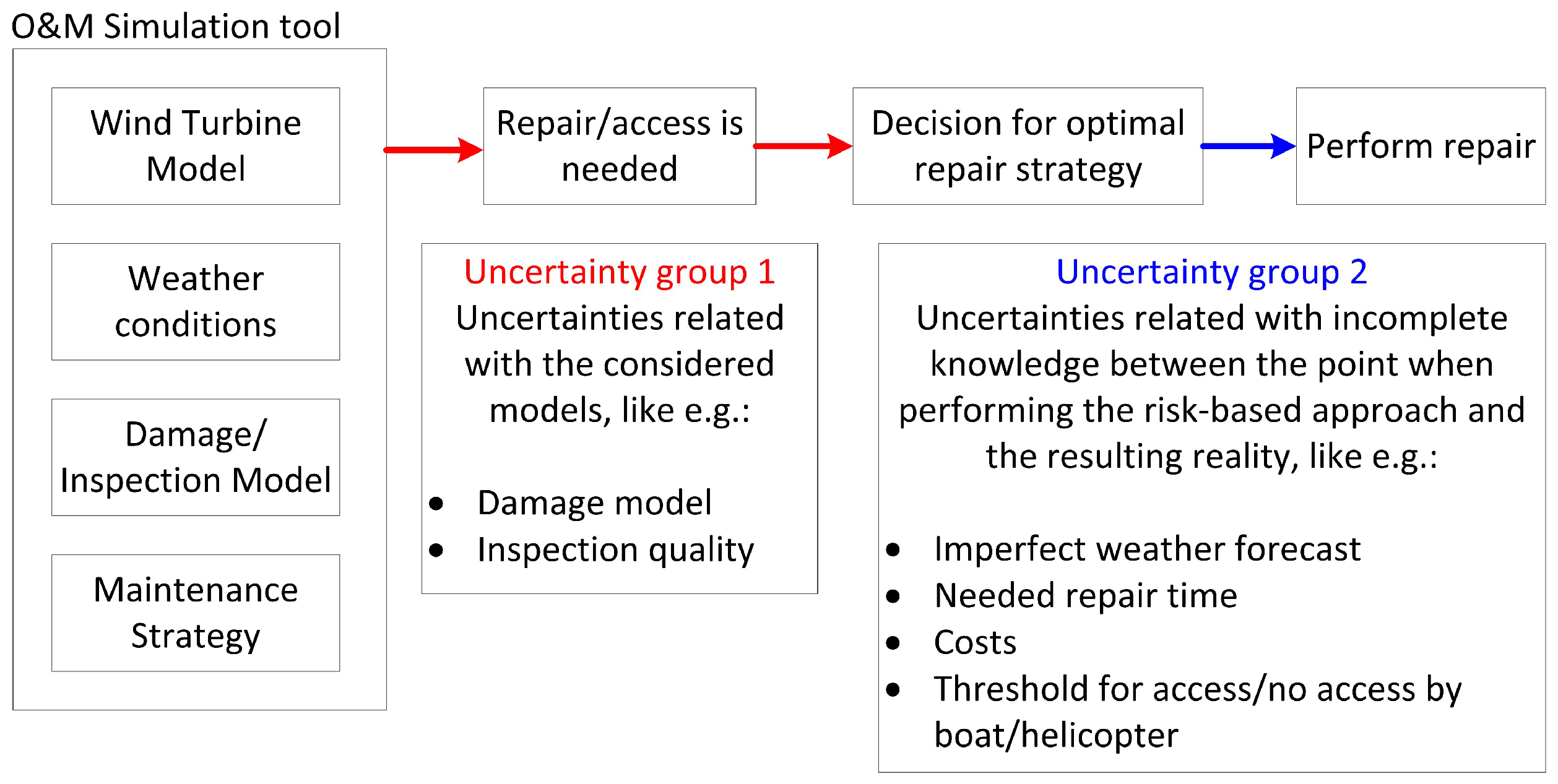
Figure 1 shows different uncertainty groups related with risk-based maintenance approaches. Uncertainty group 1 considers uncertainties related with the indication of a damage and contains e.g., damage and inspection modeling uncertainties. Uncertainty group 2 considers uncertainties related with the assumptions used as input parameters for the risk-based approach and the resulting upcoming reality. Uncertainty sources in group 2 cover imperfect weather forecasts, assumed costs, needed repair time as well as the threshold between accessibility and disability to access the device by boat or helicopter. Former studies investigate the impact of uncertainty sources in group 1 on risk-based approaches, see e.g., [7,12]. No investigation on uncertainty sources of group 2 has been performed so far.
The purpose of this paper is to make a sensitivity analysis of uncertainties from group 2 (see Figure 1) on the overall maintenance expenses by performing sensitivity studies using uncertainties from groups 1 and 2.
In this paper, Section 2 presents different maintenance strategies and the theoretical background about finding the optimal maintenance strategy, Section 4 gives information about different failure types of different components, Section 5 gives background information about the considered reference wind turbine farm and Section 6 presents the results of this study.
2. Maintenance Strategies
There are corrective and preventive maintenance strategies which can be followed when maintaining offshore wind turbines. Corrective maintenance only replaces/repairs the broken component after it breaks whereas preventive maintenance strategies try to prevent breakdown and replace the component before it breaks. Preventive maintenance can either be performed based on time (scheduled preventive maintenance) or based on the condition of the components (condition-based preventive maintenance). It needs to be kept in mind that preventive replacement can only be performed when a measure about the condition of the considered component is available.
Corrective maintenance strategies are expected to lead to a lower number of replacements compared with preventive replacements. However, the corrective replacements which cannot be scheduled and are irregular are expected to be more expensive compared with a preventive repair. However, it needs to be kept in mind that when following a preventive maintenance strategy, also corrective maintenance actions are expected to be necessary once in a while.
Transportation to the broken wind turbine can either be performed by boat or by helicopter. Access by helicopter is limited by the wind speed, and access by boat is limited by the wave characteristics. The operational costs for boats and helicopter depend, among others, on the distance between shore and wind turbine farm, the transfer time which drives the transfer time and the fuel price, as well as the hiring conditions (e.g., cost rates during waiting times in the harbor, daily/hourly rates or fixed rate operation, needed/guaranteed time for mobilization) when chartering boats and helicopters from subcontractors.
Optimal Planning of Inspection and Maintenance
Overall cost minimization over the lifetime of a wind turbine is the main target of optimal planning of maintenance and inspection actions in order to maximize the resulting benefit. Risk-based methods, which are explained in [10] for offshore wind turbine applications, are a powerful approach for finding the minimal maintenance expenses. Risk-based approaches account for risk, which is the product of the probability that a certain failure occurs and the resulting consequences. Consequences from risk calculations are only of monetary value for offshore wind turbine applications as humans are not expected to be in danger when a wind turbine fails or even collapses. Furthermore, compared with other industry branches where risk-based approaches are applied, the pollution in case of failure is small.
The procedure for finding the optimal decision making is given in Equation (1) and in Figure 2. More information about decision making for risk-based maintenance planning for offshore wind turbines can be found in [10,11,13].
Before starting with optimal planning of maintenance and inspection actions, the initial conditions of the wind turbine farm and the different wind turbines (e.g., expected lifetime, geometry, dimensions or costs) have to be defined. The range of initial conditions are seen as a matrix containing several variables and possible values. The inspection plan defining inspection and monitoring parameters like point in time to perform inspection or which inspection method to be used are defined in the matrix . After each inspection/maintenance action a random outcome, , occurs and drives the decisions for the repair plan . The decision rule is applied for future decisions on inspection results. These inspection results are uncertain at the time when the decision for the inspection plan is made. Therefore, uncertainties represented in vector like model uncertainties, environmental conditions or degradation parameters are present. These uncertainties lead to differences between planned and actual outcomes during the lifetime. The optimal strategy for initial designs, , can be found as the one that maximizes the cost function, which is the difference between the income from selling electricity and the total costs due to installations, inspections, repair, and decommissioning. The value, W, which represents the best maintenance strategy and maximizes the benefit for the wind turbine farm operator leading to the best set of initial values (z), inspection/monitoring parameters (e) and decisions (d) to be made can be calculated as (see e.g., [13]):
where B is the expected income from selling electricity, the initial investment costs, the expected service and inspection costs, the repair and maintenance costs, the expected failure costs and the decommissioning costs. When finding the optimal maintenance strategy for a wind turbine farm, the optimization problem presented in Equation (1) should be applied for the whole wind turbine farm and not a single machine.
Risk-based maintenance planning methods are stochastic approaches, where the following probabilities/uncertainties need to be considered:
- probabilities of deterioration amplification;
- probabilities of monitoring/inspection results;
- probabilities of inspection results;
- probabilities of repair (costs, required time and access possibilities).
3. Uncertainty Models
This section presents the uncertainty models developed for group 2 uncertainty sources (see Figure 1). The uncertainty models represent imperfect weather forecast, uncertain repair time on the site as well as uncertain operational range (access threshold) of the boat and helicopter.
3.1. Imperfect Weather Forecast
Weather forecasts are needed for finding weather windows enabling transportation to and from the broken wind turbine. Studies performed in [14,15] show that weather forecast uncertainty plays a central role in the number of available weather windows for performing the maintenance actions and in estimating the resulting maintenance costs.
In case the weather forecast shows excedance of the operational limits, the maintenance action needs to be postponed. In case the operational limit is exceeded during maintenance actions on sea, the maintenance action is stopped and another window needs to be found for running the remaining maintenance actions.
Weather forecasts are made based on the actual weather condition and physical/mathematical models of the atmosphere and oceans. These models can have different time lengths - from short-term weather forecast to long-term predictions about climate change. Due to the fact that weather forecasts are based among others on models, there are different reasons for uncertainties, like:
- limited number of observations;
- data errors;
- software-based and hardware-based inconsistencies between different measuring tools;
- limited time for making the forecast (trade-off between cost and quality of forecast);
- incomplete understanding about all different physical and chemical processes.
Furthermore, when talking about weather forecast uncertainties, the overall forecast uncertainty is dependent on the weather prediction horizon. A weather forecast is performed before a maintenance action is planned to be executed. Generally, the farther the forecast is, the lower the confidence and the larger the uncertainty about the weather forecast as the available information and confidence level are expected to decrease when increasing the time horizon. The weather forecast uncertainty can be considered as error term , which describes the difference between the forecasted value for time t performed at time and the actual real value at time time :
The error term represents the uncertainty about forecasting and can be assumed to be Normal distributed [16] with a bias and a standard deviation .
This model does not consider seasonal weather forecast uncertainty changes, like icing during winter periods. Table 1 shows the considered forecast uncertainties used for wind speed and significant wave height. The mean value is, as proposed by [16], set equal to 0. The time-dependent uncertainty about weather forecast standard deviation is chosen based on available forecast studies (wind: [17,18]; significant wave height [19,20,21]). Additionally an autocorrelation function is considered here in order to represent correlation between the successively following wind speeds and significant wave height values and preventing large variations, which is physically unrealistic, among values behind each other. This uncertainty model can be used for weather forecast uncertainty modeling for risk-based planning of maintenance actions. Figure 3 gives an example of a two-day weather forecast taking the model explained in Equation (3) and the model values shown in Table 1 into account.
3.2. Uncertain Repair Time
The repair time on the site itself is considered as a stochastic variable () due to the fact that there are different severities and failure levels (from minor to major), which will use different numbers of days on the site to be repaired. The number of repair days on site is used as input parameter for the risk-based maintenance approach. However, the considered needed days for repair might not always be the number of days that the technicians really need to fix the failure as unforeseen problems can occur or the technicians can repair the failure faster as expected. Therefore, an uncertainty factor, , which models the difference between the expected number of days for repair and the real used number of days on site is introduced here. The real needed number of days to repair the failure, , can be modeled in the following way:
where is the number of repair days considered for estimating the costs for risk-based maintenance approach. The uncertainty, , about the repair times can, according to [15], be assumed to be Lognormal distributed in order to prevent negative repair times. The mean value of is equal to or larger than 1. In case of using conservative estimates on the duration, a bias larger than 1 can be relevant.
3.3. Uncertain Operational Range Limitations of Boat and Helicopter
In research, one often defines operational range limitations of boats and helicopters with e.g., the maximum significant wave height or maximum wind speed for operational actions. However, these values are, once on sea, impossible to detect accurately. Additionally, not a sharp threshold between access and no access as considered in most maintenance studies, exists but accessibility also depends on the skills of the crew.
When performing maintenance actions, human factors like the experience and risk willingness of the supply vessel skipper or helicopter pilot play important roles. This not only means that the significant wave height as well as the wind speed give a threshold about accessibility to the wind turbines, but also other aspects, which are not considered in the simplified operational range definition in Section 5.4, like the steepness of the waves for the boat and the turbulence intensity for the helicopter as well as the physical response of the equipment to be transported as explained in [22].
The operational range uncertainty can be assumed to be small for small maintenance boats, as considered in this study, but becomes more important for installation purposes where big ships and cranes are used. The uncertainty about human risk and experience might be quite scattered among different captains/pilots. Therefore, it is very difficult to quantify this uncertainty source in numbers. A sensitivity study is performed assuming that the origin of operational range limitations is based on the uncertain detection of wave characteristics on sea (wrong estimation of significant wave height and wind speed).
The model in order to assess the cost impact on access uncertainty is based on a stochastic variable modeling the access threshold (significant wave height or wind speed) at the site, which is dependent on the deterministic threshold value considered in the risk-based approach as well as a Normal distributed parameter , which represents the incomplete knowledge about repair time needed on site:
where represents the deterministic threshold for having access by boat/helicopter considered for risk-based maintenance planning. The parameter has a mean value equal to 1 and a standard deviation . This parameter can be due to lack of data and experience assumed to be presented by a simple Normal distribution.
4. Failure Types and Their Corresponding Models
Failures of mechanical as well as electrical components and software failures happen in different ways. These differences need to be accounted for when doing maintenance cost estimations.
4.1. Mechanical Failures—Damage Model
Failure of mechanical components are based on mechanical procedures leading to failures. Critical for most mechanical components used in offshore wind turbines is cyclic loading (wear or fatigue). This procedure can be mathematically described as a time-dependent deterioration process. Examples of mechanical components are the blades, the gearboxes or the shafts. Inspections and monitoring systems can indicate future mechanical failure as deterioration is shown e.g., by cracks (inspections) or vibrations (monitoring).
Mechanical failures can be modeled with damage accumulation models that estimate the component condition at each time step. The model considered in this article is based on the model shown in [7,13,23]. The damage model considered in this section implies fatigue cracking. However, also other kinds of time-dependent damages like corrosion or wear can be modeled using the explained approach. The general equation representing the damage size D is given as:
where represents the damage growth, F a load measure and D is the damage size. The parameters C, and are model parameters, which can be estimated from available failure rates. The damage size D reaches numbers between 0 and 1. When the damage size reaches 1, failure of the considered component occurs and needs to be repaired/replaced. Paris Law [24] can be used to calculate the damage accumulation rate :
where C is the damage coefficient, m the damage exponent and the damage intensity factor, which, among others, depends on the actual damage D and can be calculated using the following equation:
where is the cyclic damage range and the geometry factor. The damage coefficient C and the damage exponent m from Equation (6) can be calibrated from available failure rates of the corresponding components or directly taken from already performed studies like [7,13,23]. The cyclic damage is in this study assumed to be proportional to the mean significant wave height as done in other studies, like [7,13]) with focus on offshore wind turbine applications. Furthermore, the mean zero-crossing wave period, , is assumed to drive the number of cycles N per time step, which is indicated as in Equation (7).
Inspections and repair/replacement of a damaged component are performed when the detected damage is larger than a certain threshold . Replacements when detecting damages during inspections will take place when the detected damage is larger than a certain threshold , which indicates the minimal necessary damage that repair/replacement is performed. When performing inspections not all damages might be detected. This fact needs to be accounted for when modeling inspections. Inspections can be modeled using so-called probability of detection curves (s). These curves show the probability of detection dependent on the damage size and the used inspection technique. Different curves are presented in [25]. One possibility of defining such a probability of detection curve is by using a one-dimensional exponential threshold model, see e.g., [7,13,25]:
where D is the actual damage, the maximum probability of detection and the expected value of smallest detectable damage.
There exist different inspection strategies: performing inspections with pre-defined inspection intervals (intervals fixed over lifetime or dependent on the damage result from former inspections) or condition-based inspections where inspections are performed based on failure indication from the monitoring system.
4.2. Electrical/Software Failures—Failure Rates
For electrical component failures or software failures no deterioration model as presented in Equation (6) can be used as these failure types occur randomly in time. Software failures can often be solved by manual restarts or updates of the operating system/software using online access. Electrical failures make access by technicians to the device necessary, as these failures need exchange/repair of components. A common way to model electrical and software failures is by using so-called annual failure rates . These failure rates model the expected (mean) failure rate over one year. The annual failure rate from a data set of failure reports can be estimated based on [13,26]:
where is the number of failures, N is the component population and T indicates the operational period (in years). There exist failure rate databases developed for offshore wind turbine applications like [27,28,29,30]. Failure rate studies for offshore wind turbine applications are performed in [26,31,32]. Furthermore, databases from the the petrochemical industry (see e.g., [33]) or generic reliability databases like [34,35] could be used for failure rate estimations.
5. Case Study
The case study considers a wind turbine farm consisting of ten 6 MW wind turbines, which are placed 30 km off the Danish coast. Figure 4 shows the considered power curve of the reference offshore wind turbine, which is similar to the 6 MW Senvion wind turbine. All wind turbines are assumed to operate under free flow conditions without wake conditions from other wind turbines. The study presented in [13] considers the same wind turbine farm layout and reference wind turbine.
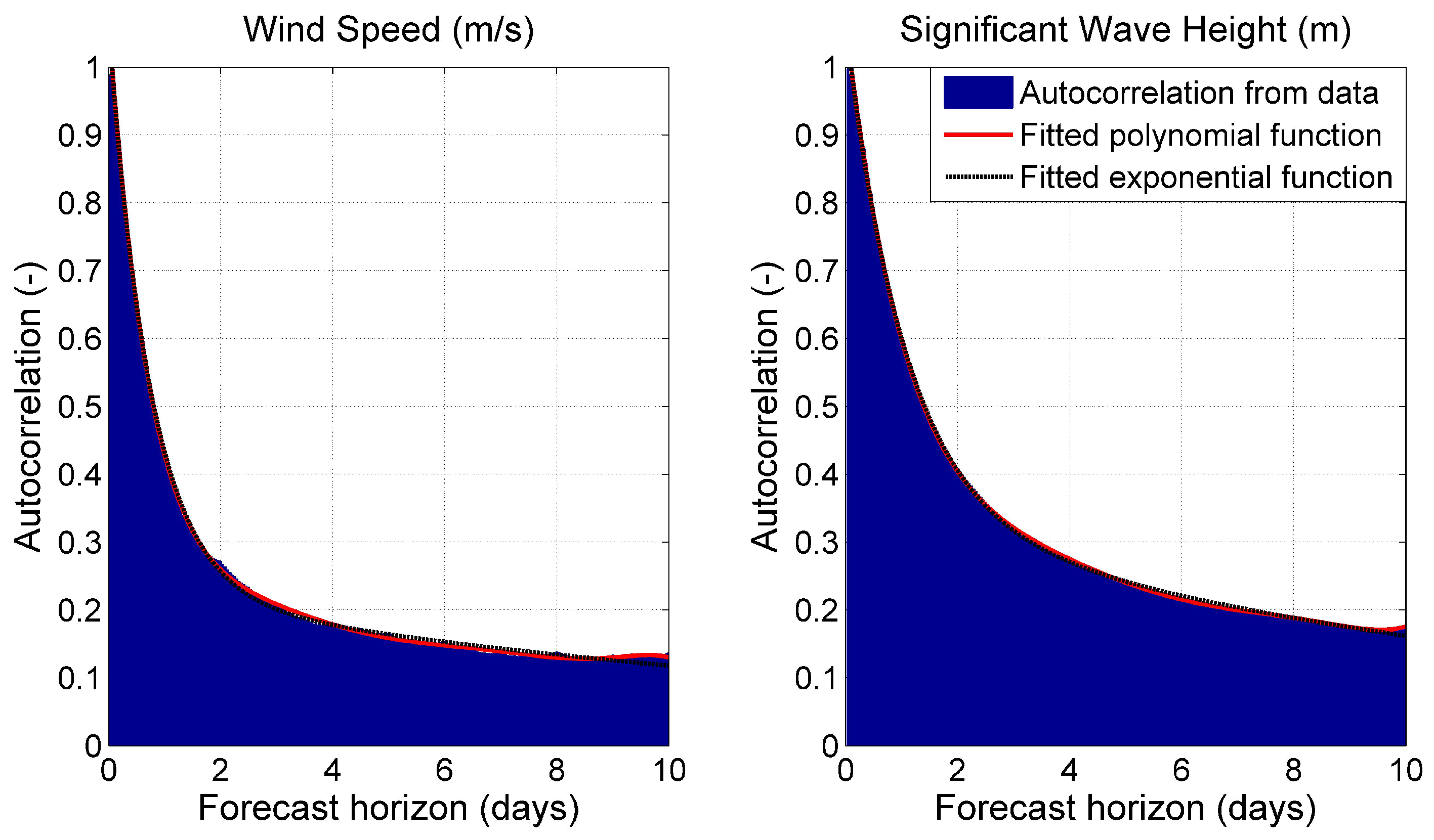
Real weather data (available between 1979 and 2009) is considered for this study. More detailed information about the wind speed distribution and the significant wave height as well as the zero-crossing wave period can be seen in [13]. The autocorrelation of wind speed and significant wave height considered in this case study is based on the autocorrelation estimation, taking all 31 years of weather data into account. Figure 5 shows the resulting correlation coefficients for the mean wind speed and the significant wave height. A polynomial function with 7 degrees as well as a two-term exponential function are fitted to the resulting autocorrelation results. The polynomial fit shows better fit for high time horizons whereas for small forecast horizons the difference between the fits is negligible.
The reference wind turbine in this study is simplified with respect to the number of considered components. Figure 6 shows the main components of which the considered wind turbine consists of. The expected lifetime of the wind turbines is 20 years. Crude Monte Carlo simulations are considered in order to estimate the expected total maintenance costs and repairs during one lifetime. This study considers the following three different maintenance strategies:
- only corrective maintenance actions;
- preventive and corrective maintenance actions with a fixed inspection interval of 0.5 years;
- preventive and corrective maintenance actions based on alarms from a condition monitoring system.
Reference [13] considers the same maintenance strategies for a maintenance study of casted components mounted on the drive train of the 6 MW reference wind turbine. Failures at a wind turbine can have different severity levels. There are minor failures, which contain failures of electrical and mechanical components and can be replaced on the site by either exchanging a sub-component or simply repair the broken part. However, also major failures which may lead to total or partial collapse of the wind turbine as well as secondary damages may occur. For these severe damages of large structural parts like the tower or the foundation, large transportation vessels and jack-up crane vessels may be needed. This study only considers minor failures. It is assumed that the electricity feed-in tariff is equal to 0.08 €/KWh, which is according to [36] a common value for fixed feed-in tariffs for offshore wind turbine farms.
5.1. Considered Failure Data
This section describes the considered failure rates as well as damage parameters used in the damage model presented in Section 4. Recent studies show annual failure rates of offshore wind turbines in the range between 6 and 9.5 failures per year: [3]: 9.5 failures/year/turbine; [31]: 8 failures/year/turbine (without major repairs) and [37]: 6 failures/year/turbine. In this study for calibrating the damage model and the software/electrical failure rates an overall annual failure rate of 9 incidents per year is considered.
Mechanical failures in this study are modeled using the model proposed in Section 4.1. The mechanical damage model parameters mean value of C (damage coefficient) and (proportionality factor) are calibrated by using available annual failure rates of these mechanical components, which are considered in [13] and originally taken from [3,27,31]. Table 2 shows the considered damage values for different mechanical components. The stochastic parameters C and are assumed to be Lognormal distributed [7]. The damage exponent m and the geometry factor are considered in this case study as deterministic values [13]. It is assumed that all mechanical components have an initial damage, , which is assumed to be exponentially distributed with mean value equal to 0.02 and a coefficient of variation of 0.02, as considered in the studies performed by [7] and [13].
Failure of electrical components as well as software failure are modeled based based on failure rates, as explained in Section 4.2. Table 3 shows the considered failure rates taken from [13] for software problems and failure of electrical components mounted at the reference offshore wind turbine.
Due to the fact that the considered simplified wind turbine model as shown in Figure 6 does not cover all components, the estimated failure rates considered in [13] are adapted from the original failure rate sources [3,27,31] such that the sum of considered failure rates reach 9 failures per year.
If an electrical or mechanical component fails, a technician crew needs to access the wind turbine in order to fix the problem. When a software failure occurs, it is assumed that the technicians can access the software online and by updating or restarting the controller the problem can be solved.
5.2. Parameters for Inspection and Maintenance Modeling
Inspections are performed to identify future failures of mechanical components by detecting cracks. Inspections are modeled with so-called curves (see Equation (9)). The considered curve parameters, which are taken from [13], are shown in Table 4.
It is assumed in this study that the curve is the same for all mechanical components during the inspection as the same crew is inspecting the different mechanical components as well as the same inspection method is used for all mechanical components. In this example visual inspection is considered to be performed. The smallest detectable damage, , represents human errors and measurement uncertainties. Therefore, is modeled as stochastic variable which is Normal distributed with a coefficient of variation (COV) equal to 0.1 [7]. It needs to be mentioned that when modeling other inspection methods, the smallest detectable damage, needs to be adjusted. The decision rule for repair given a detection of a crack, which is represented by , as well as parameters of the curve are assumed to stay constant over the whole lifetime.
More details about the chosen inspection and maintenance parameters are given in [13].
5.3. Considered Costs
Failure of mechanical and electrical components make access to the wind turbine necessary. The total repair costs for a corrective repair of electrical and mechanical components consist of the transportation cost, the costs for working hours on the site as well as the cost for the material (new component or repaired component) and the downtime of the wind turbine leading to lost production including the waiting time due to bad weather conditions. Transportation costs can be shared when several components can be repaired with the same journey. Preventive replacements are performed during inspections. When performing inspections, the overall inspection costs consist of the transportation costs, the actual downtime (lost electricity production) while inspection is ongoing as well as the repair costs when a crack is detected.
Table 5 shows the expected material costs for the different mechanical and electrical components for repairing a failure. The cost data for a 6 MW offshore wind turbine presented in Table 5 is already considered in [13].
Table 6 shows the number of days needed on the device for different failures. This study only considers full days for repair since equipment (e.g., boat and technicians) is often rented on a daily basis. This means the stochastic variable can only get integer values and no lower values than 1. The mean value of (see Equation (5)) is in this case study assumed to be 1. If the weather allows it, repairs are able to be started the following day after failure occurrence at 6:00 in the morning.
Software failures are assumed to be solved by restarting the machine or installing a software update. This means that software failures can be solved relatively quickly compared with failures of electrical or mechanical components. The costs which result from software repairs are the labor costs needed to analyze the problem and restart the machine. In this case study, it is assumed that a wind turbine with a software failure can resume service after one working day [13], after two specialists were working on fixing the software problem.
Table 7 shows the considered transportation and inspection costs. These cost assumptions are taken from [13]. An interest rate of 5% is considered in this study, as also considered in other studies performed by [7,13,37].
When the weather conditions are too bad to fly or sail to the broken wind turbines, the cost of waiting is represented by lost electricity production. No additional costs (e.g., waiting fees) are considered in this study when the boat or the helicopter needs to wait due to bad weather conditions. Furthermore, it is assumed that the boat as well as the helicopter are always available and the daily hiring costs are constant over the whole lifetime. Inspections are always performed by boat. The same cost assumptions as presented in this section have been considered in the case study presented in [13] where more detailed information about cost assumptions can be found.
5.4. Considered Operational Range of Boat/Helicopter
Transportation to the wind turbines is either done by boat or helicopter. According to [13] is access by boat mainly limited by the wave height (given a limitation of significant wave height) and the maneuverability of the helicopter as well as safe lowering of personnel and material is limited by the wind speed. Reference [39] highlights that the comfort during transportation on the water is affected by the waves. High waves have the risk that the technicians suffer from sea sickness. The common limitations (boat: [7,13,37]; helicopter: [7,13,40]) for boat and helicopter operations are the following:
Accessibility is not only limited by the significant wave height and the wind speed, respectively. However, also other factors like humidity and temperature leading to limited visibility due to fog or wind directions as well as wave periods may limit the access. This effect of having multiple reasons for access limitations is studied in the results when adding accessibility uncertainties. Furthermore, the above mentioned access limitations are not strict but depend on the pilot and captain’s skills and risk taking.
6. Results
The impact on the total maintenance expenses of the following uncertainties, which represent uncertainty group 2 in Figure 1, are considered in this section when optimizing maintenance planning using a risk-based approach:
- weather forecast;
- assumed repair time on site;
- operational range of helicopter/boat.
The aforementioned uncertainties are first considered individually and then combined in order to estimate common effects. For all performed simulations also uncertainties from group 1 like uncertainty of the damage model as well as the inspection quality (see Section 4.1) are considered.
6.1. Sensitivity of Weather Forecast
In order to assess the impact of weather forecast uncertainties, the model presented in Section 3.1 together with the fitted autocorrelation factor shown in Section 5 is considered. Figure 7 shows the impact of considering weather forecast uncertainty on the total maintenance expenses for different maintenance strategies (corrective/preventive) when following a risk-based transportation strategy. Imperfect knowledge about the weather conditions in the future mainly impacts the amount of lost electricity production due to longer down times of the broken wind turbines. The largest increase in total maintenance costs when considering weather forecast uncertainty happens following a corrective maintenance strategy. Then, the total maintenance costs are roughly 1.74 times higher than without taking weather forecast uncertainties into account. For preventive maintenance strategies, the increase is 56% for regular inspections and 35% when using a condition monitoring system.
Table 8 gives a more detailed overview about important key parameters like availability or ratio of maintenance expenses of the electricity prize as well as the COV of the expected total maintenance expenses shown in Figure 7. When considering no weather forecast uncertainty, the availability of the considered offshore wind turbines is in the range of 90%–93% whereas this value decreases to 74%–83% when taking weather uncertainties into account. Also the operation and maintenance expenses increase from 0.012–0.016 €/KWh to 0.017–0.034 €/KWh when considering weather uncertainties. On the other hand, the COV values reach between 0.21 and 0.25 when assuming imperfect weather forecast compared with COV values between 0.06 and 0.07 when perfect weather forecast is assumed.
Furthermore, the sensitivity of the quality of the weather forecast is analyzed by adapting the weather forecast uncertainty. Figure 8 shows the impact of weather forecast uncertainty on the total expected maintenance costs for the whole wind turbine farm during a lifetime of 20 years. Bad weather forecast represents forecasts with a 20% larger uncertainty than the uncertainty shown in Table 1, which corresponds to the normal weather forecast case. A good weather forecast assumes a 20% lower uncertain than the normal weather forecast. The total maintenance expenses decrease, as expected, when increasing the weather forecast accuracy, and the overall maintenance expenses are very sensitive on the weather forecast uncertainty.
6.2. Sensitivity of Assumed Operational Range of Boat/Helicopter
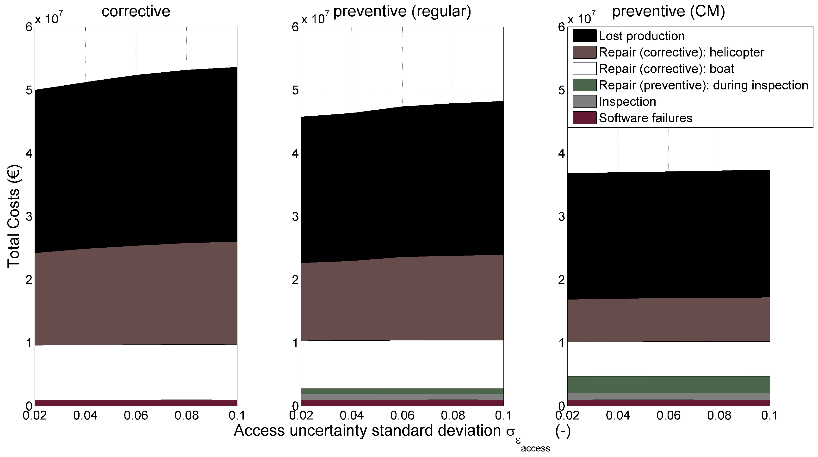
Figure 9 shows the impact of operational range limits by boat and helicopter on the total expected maintenance expenses for different maintenance strategies. The operational range uncertainty is, according to Equation (5), represented by a Normal distributed parameter . Its standard deviation is adapted between 0.02 and 0.1 in this study. The total expected maintenance expenses only slightly increase when increasing the standard deviation . The increased maintenance expenses result from operations where no access to the device was possible and the boat or helicopter had to travel back to the harbor without performing the repair. This leads to longer waiting times as well as another attempt to access the wind turbine is necessary.
6.3. Sensitivity of Time to Repair on Site
This section investigates the impact of the uncertainty about the repair time needed on site considered for the risk-based decision-making. The uncertainty model presented in Section 3.2 is considered for modeling the repair time uncertainty.
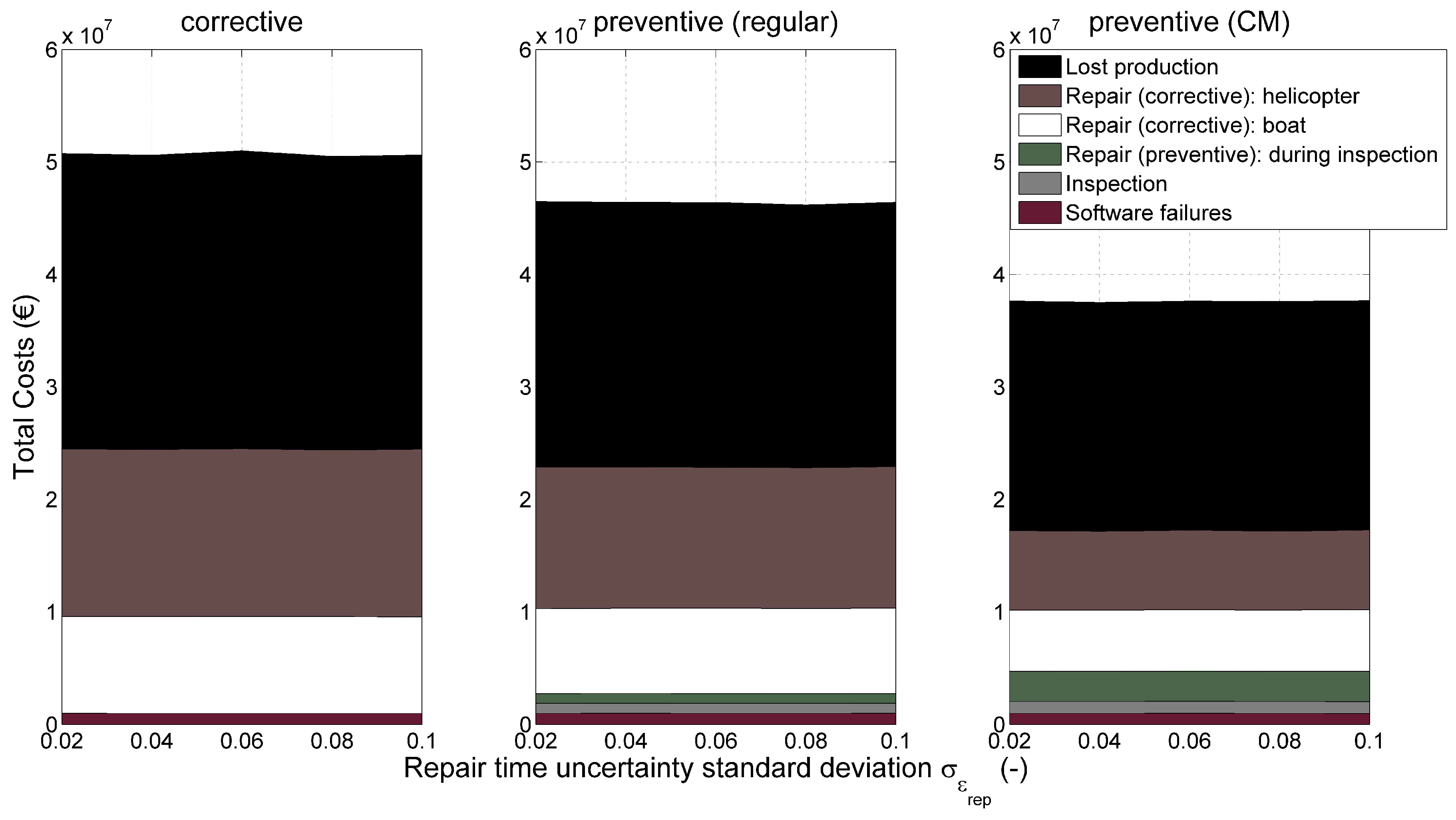
Figure 10 shows the expected total maintenance costs of the considered reference wind turbine farm over a lifetime of 20 years dependent on the uncertainty level of the repair time used on the site to repair the broken components. Different uncertainty levels of the needed repair time on site is represented by different repair time uncertainty standard deviations, . It can be seen that there is no significant change on maintenance expenses when changing the uncertainty level of the repair time. The maintenance costs are the same for different values as without considering any repair time uncertainty.
6.4. Sensitivity of Combination of the Different Uncertainty Sources
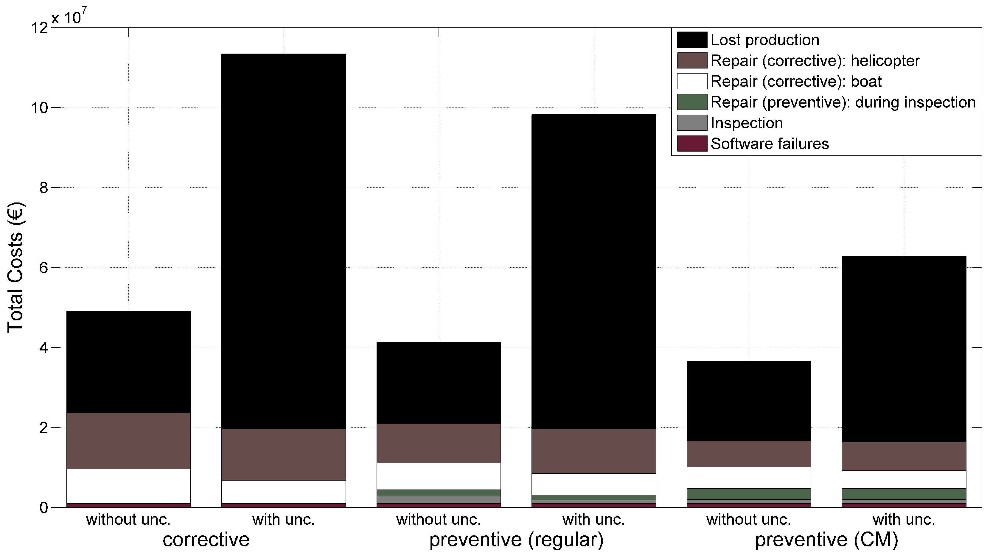
Figure 11 shows the resulting maintenance costs over a lifetime of 20 years when considering all afore-mentioned uncertainties related with risk-based maintenance planning. Reference [41] considered an envelope of ±20% for downtime uncertainties. When assuming that represents the whole sample space, this leads to a standard deviation of roughly 0.07, which is considered the value considered for in Figure 11. The standard deviation, , is chosen to be 0.05. The maintenance expenses are increasing when considering uncertainties related to weather forecast, repair time on site as well as the access uncertainty of the boat and the helicopter. The main reason for increased maintenance expenses is due to longer waiting time, which leads to larger loss of electricity production costs.
Table 9 shows the availability, maintenance expenses per produced KWh of electricity and coefficient of variation of expected maintenance costs as ratio between the case where uncertainties related with risk-based maintenance planning are considered and the case without any risk-based decision related uncertainties taken into consideration. The expected maintenance costs increase by 72% to 138% when taking uncertainties related with risk-based decision-making into consideration. The availability decreases between 11% to 32% when including risk-based maintenance planning uncertainties. The fluctuation of total maintenance expenses among different simulations are increased by roughly a factor of 3 to 4. When using a condition monitoring system, the effects on maintenance costs, availability reduction, and maintenance cost fluctuations are lowest compared with regular preventive and corrective maintenance strategies.
The previously mentioned differences are large and show the importance of considering uncertainties related to risk-based decision-making for maintenance planning of offshore wind turbine farms. The study presented in [15] where uncertainties on the weather forecast and repair time are summarized in one stochastic variable shows that the lost production is increased by 100% to 150% when following a corrective maintenance strategy compared with deterministic values for repair time on the site and weather forecasts. Additionally, the availability decreased by roughly 35%–45% when considering repair time uncertainties and weather model uncertainties. The presented numbers in [15] are in accordance with the results presented in Figure 11 and Table 9.
7. Conclusions
Many research publications show that risk-based maintenance planning makes it possible to decrease the overall maintenance expenses for an offshore wind turbine farm. However, risk-based optimal maintenance planning needs a lot of knowledge about input parameters, which often are not completely known. This incomplete knowledge is a potential risk for taking the wrong decision based on wrong input parameters and not including all uncertainties related to it. The problem to be answered in this paper is related to the resulting maintenance costs when not having complete knowledge about all input parameters needed to find the maintenance strategy leading to the lowest overall maintenance costs following risk-based maintenance planning.
A case study is considered assuming a wind turbine farm with ten 6 MW wind turbines placed 30 km off the Danish North Sea shore. Sensitivity studies on uncertainties related with weather forecasts, incomplete knowledge about the time needed on site to repair the broken component as well as the uncertain threshold limiting accessing the wind turbine by boat or helicopter used for risk-based maintenance planning approaches are performed in the case study. The considered uncertainty levels considered in the case study are estimated from former studies studies (damage model uncertainty, inspection modeling uncertainty and repair time on the site uncertainty), estimated based on data (weather forecast uncertainty) or an uncertainty range is defined by the authors (operational range of boat/helicopter). Furthermore, different maintenance strategies like corrective or preventive (scheduled and condition-based) are considered and the overall expected maintenance costs are estimated based on Crude Monte Carlo simulations.
The study showed that the uncertainty about weather forecast can drastically increase the costs for maintenance expenses, and therefore accurate and reliable weather forecasts are of great importance. The uncertainty about the repair time on the site has no influence on the expected total maintenance costs, and the expected total maintenance expenses only increase slightly when increasing the level of access uncertainty. When considering all three uncertainty sources related to risk-based maintenance planning, the total expected maintenance expenses increase between 72% to 138% for the considered reference wind turbine park. The main reason for increased maintenance cost is mainly due to longer waiting times. The availability is decreasing between 11% to 32% when considering the afore-mentioned uncertainties compared with no risk-based decision-making uncertainty consideration. The lowest impact on cost increase and availability decrease is reached when using a condition monitoring system to detect possible failures. The largest overall cost increase when adding uncertainties happens when following a corrective maintenance strategy.
The presented costs and cost-saving potentials among different maintenance strategies is, among others, site-dependent as well as wind turbine (farm) dependent. A next step for improving the considered simulation tool could be to implement learning curves and improvements in decision theory during the lifetime. These improvements will most probably decrease the total maintenance costs. Therefore, the presented costs are only valid for the assumptions made in the case study and are expected to be different for other wind turbine farms.
Acknowledgments
The authors wish to thank the financial support from the Danish Council for Strategic Research (Grant No. 10-093966, REWIND—Knowledge based engineering for improved reliability of critical wind turbine components) which made this work possible.
Author Contributions
The main idea for the paper was proposed by Simon Ambühl and John Dalsgaard Sørensen. Simon Ambühl wrote the first paper draft of the paper. John Dalsgaard Sørensen thoroughly reviewed the paper and Simon Ambühl revised the paper.
Conflicts of Interest
The authors declare no conflict of interest.
References
- Yeng, Y.; Tavner, P.; Long, H. Early experiences with UK round 1 offshore wind Farms. Proc. Inst. Civ. Eng. Energy 2010, 163, 167–181. [Google Scholar]
- Musial, W.; Ram, B. Large-Scale Offshore Wind Power in the United States: Assessment of Opportunities and Barriers; NREL/TP-500-40745; National Renewable Laboratory: Denver, Co, USA, 2010.
- Maples, B.; Saur, G.; Hand, M.; van de Pietermen, R.; Obdam, T. Installation, Operation, and Maintenance Strategies to Reduce the Cost of Offshore Wind Energy; NREL/TP-5000-57403; National Renewable Laboratory: Denver, CO, USA, 2013.
- Hofmann, M. A review of decision support models for offshore wind farms with an emphasis on operation and maintenance strategies. Wind Eng. 2011, 35, 1–16. [Google Scholar] [CrossRef]
- Arunraj, N.S.; Maiti, J. Risk-based maintenance—Techniques and applications. J. Hazard. Mater. 2006, 142, 653–661. [Google Scholar] [CrossRef] [PubMed]
- Faber, M.; Stewart, M.G. Risk assessment for civil engineering facilities: Critical overview and discussion. Reliab. Eng. Syst. Saf. 2003, 80, 173–184. [Google Scholar] [CrossRef]
- Nielsen, J.J.; Sørensen, J.D. On risk-based operation and maintenance of offshore wind turbine components. Reliab. Eng. Syst. Saf. 2011, 96, 218–229. [Google Scholar] [CrossRef]
- Florian, M.; Sørensen, J.D. Wind turbine blade life-time assessment model for preventive planning of operation and maintenance. J. Mar. Sci. Eng 2015, 3, 1027–1040. [Google Scholar] [CrossRef]
- Brennan, F. Risk based maintenance for offshore wind structures. Procedia CIRP 2013, 11, 296–300. [Google Scholar] [CrossRef]
- Sørensen, J.D. Framework for risk-based planning of operation and maintenance for offshore wind turbines. Wind Energy 2009, 12, 493–506. [Google Scholar] [CrossRef]
- Nielsen, J.S.; Sørensen, J.D. Methods for risk-based planning of O&M of wind turbines. Energies 2014, 7, 6645–6664. [Google Scholar]
- Rangel-Ramirez, J.G.; Sørensen, J.D. Risk-based inspection planning optimisation of offshore wind turbines. Struct. Infrastruct. Eng. 2012, 8, 473–481. [Google Scholar] [CrossRef]
- Ambühl, S.; Sørensen, J.D. On Different Maintenance Strategies for Casted Components of Offshore Wind Turbines; DCE No. 222; Aalborg University: Aalborg, Denmark, 2017. [Google Scholar]
- Gintautas, T.; Sørensen, J.D. Evaluating a novel approach to reliability based decision support for offshore wind turbine installation. In Proceedings of the 2nd International Conference on Renewable Energies Offshore, Lisbon, Portugal, 24–26 October 2016; pp. 733–740. [Google Scholar]
- Seyr, H.; Muskulus, M. Value of information of repair times for offshore wind farm maintenance planning. J. Phys. Conf. Ser. 2016, 753, 092009. [Google Scholar] [CrossRef]
- Lange, M. On the uncertainty of wind power predictions—Analysis of the forecast accuracy and statistical distribution of error. J. Sol. Energy Eng. 2005, 127, 177–184. [Google Scholar] [CrossRef]
- Möhrlen, C. Uncertainty in Wind Energy Forecasting. Ph.D. Thesis, University College Cork, Cork, Ireland, 2004. [Google Scholar]
- Ko, W.; Hur, D.; Park, J.-K. Correction of wind power forecasting by considering wind speed forecast error. J. Int. Counc. Electr. Eng. 2015, 5, 47–50. [Google Scholar] [CrossRef]
- Babovic, V.; Sannasiraj, S.A.; Chan, E.S. Error correction of a predictive ocean wave model using local model approximation. J. Mar. Syst. 2015, 53, 1–17. [Google Scholar] [CrossRef]
- Natskår, V.; Moan, T.; Alvær, P.Ø. Uncertainty in forecasted environmental conditions for reliability analyses of marine operations. Ocean Eng. 2015, 108, 636–647. [Google Scholar] [CrossRef]
- Wilcken, S. Alpha Factors for the Calculation of Forecasted Operational Limits for Marine Operations in the Barents Sea. Master’s Thesis, University of Stavanger, Stavanger, Norway, 2015. [Google Scholar]
- Gintautas, T.; Sørensen, J.D.; Vatne, S.R. Towards a risk-based decision support for offshore wind turbine installation and operation & maintenance. Energy Procedia 2016, 94, 207–217. [Google Scholar]
- Ambühl, S.; Kofoed, J.P.; Sørensen, J.D. Operation and maintenance strategies for wave energy converters. Inst. Mech. Eng. Proc. Part O J. Risk Reliab. 2015, 229, 417–441. [Google Scholar] [CrossRef]
- Paris, P.C.; Erdogan, F. A critical analysis of crack propagation laws. J. Basic Eng. 1963, 85, 528–533. [Google Scholar] [CrossRef]
- Straub, D. Generic Approaches to Risk-Based Inspection Planning for Steel Structures. Ph.D. Thesis, Swiss Federal Institute of Technology—ETH Zurich, Zurich, Switzerland, 2004. [Google Scholar]
- Tavner, P.J.; Xiang, J.; Spinato, F. Reliability analysis of wind turbines. Wind Energy 2007, 10, 1–18. [Google Scholar] [CrossRef]
- Wilkinson, M.; Harman, K.; Hendriks, B.; Spinato, F.; van Delft, T. Methodology and results of the ReliaWind reliability field study. In Proceedings of the Scientific Track Proceedings: European Wind Energy Conference, Warsaw, Poland, 20–23 April 2010. [Google Scholar]
- Van Brussel, J.W.; Zaaijer, M.B. Estimation of Turbine Reliability Figures within the DOWEC Project; Dutch Offshore Wind Energy Converter (DOWEC), ECN: Petten, The Netherlands, 2003. [Google Scholar]
- Ribrant, J.; Bertling, L.M. Survey of failures in wind power systems with focus on Swedish wind power plants during 1997–2005. IEEE Trans. Energy Convers. 2007, 22, 167–173. [Google Scholar] [CrossRef]
- IEA Wind Task 33. Reliability Data Standardization of Data Collection for Wind Turbine Reliability and Operation & Maintenance Analyses; International Energy Agency (IEA): Geneva, Switzerland, 2012. [Google Scholar]
- Carroll, J.; McDonald, A.; McMillian, D. Failure rate, repair time and unscheduled O&M cost analysis of offshore wind turbines. Wind Energy 2016, 19, 1107–1119. [Google Scholar]
- Faulstich, D.; Hahn, B.; Tavner, B.J. Wind turbine downtime and its importance for offshore deployment. Wind Energy 2011, 14, 327–337. [Google Scholar] [CrossRef]
- Offshore and Onshore Reliability Data (OREDA) Project. Offshore Reliability Data Handbook; SINTEF and OREDA Participants: Trondheim, Norway, 2009. [Google Scholar]
- IEE Std 500-1984. Reliability Data for Pumps and Drivers, Valve Actuators and Valves; Institute of Electrical and Electronics Engineers (IEEE): New York, NY, USA, 1984. [Google Scholar]
- MIL-HDBK-271F. Military Standardization Handbook—Reliability Prediction of Electronic Equipment; Department of Defense: Washington, DC, USA, 1991.
- Green, R.; Vasilakos, N. The economics of offshore wind. Energy Policy 2010, 39, 496–502. [Google Scholar] [CrossRef]
- Dalgic, Y.; Lazakis, I.; Turan, O. Investigation of optimum crew transfer vessel fleet for offshore wind farm maintenance operations. Wind Eng. 2015, 39, 31–52. [Google Scholar] [CrossRef]
- Poore, R.; Walford, C. Development of an Operations and Maintenance Cost Model to Identify Cost of Energy Savings for Low Wind Speed Turbines; NREL/SR-500-40581; National Renewable Laboratory: Denver, CO, USA, 2008.
- Logistics Efficiencies and Naval Architecture for Wind Installations with Novel Developments (LEANWIND) Project. Work Package 3—Deliverable 3.1—Novel Vessels and Equipment; University College Cork: Cork, Ireland, 2014. [Google Scholar]
- Bierbooms, W.A.A.M.; van Bussel, G.J.W. The impact of different means of transport on the operation and maintenance strategy for offshore wind farms. In Section Wind Energy, Faculty Civil Engineering and Geosciences; Delft University of Technology: Delft, The Netherlands, 2002. [Google Scholar]
- Martin, R.; Lazakis, I.; Barbouchi, S.; Johanning, L. Sensitivity analysis for offshore wind farm operation and maintenance cost and availability. Renew. Energy 2016, 85, 1226–1236. [Google Scholar] [CrossRef]
Figure 1.
Flow chart showing the different uncertainty groups when performing maintenance simulations using a risk-based approach.
Figure 1.
Flow chart showing the different uncertainty groups when performing maintenance simulations using a risk-based approach.

Figure 2.
Decision tree for optimal planning of operation and maintenance actions [10].
Figure 2.
Decision tree for optimal planning of operation and maintenance actions [10].
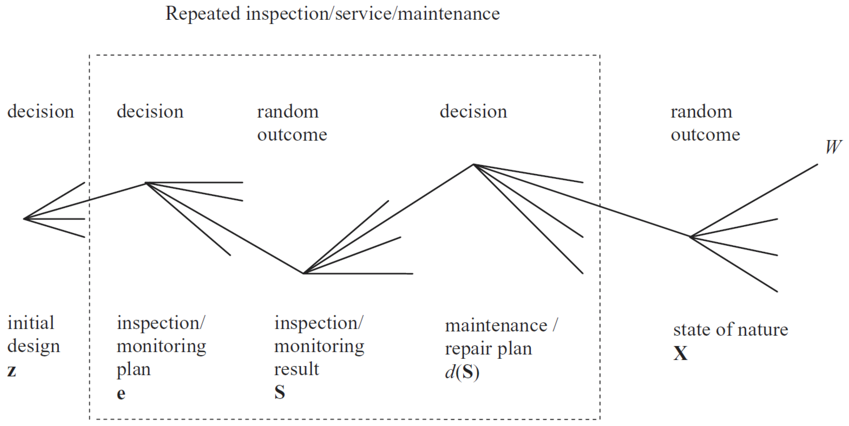
Figure 3.
Example of a 48-h wind speed and significant wave height forecast based on the model explained in Table 1 and Equation (3). dev.: deviation.
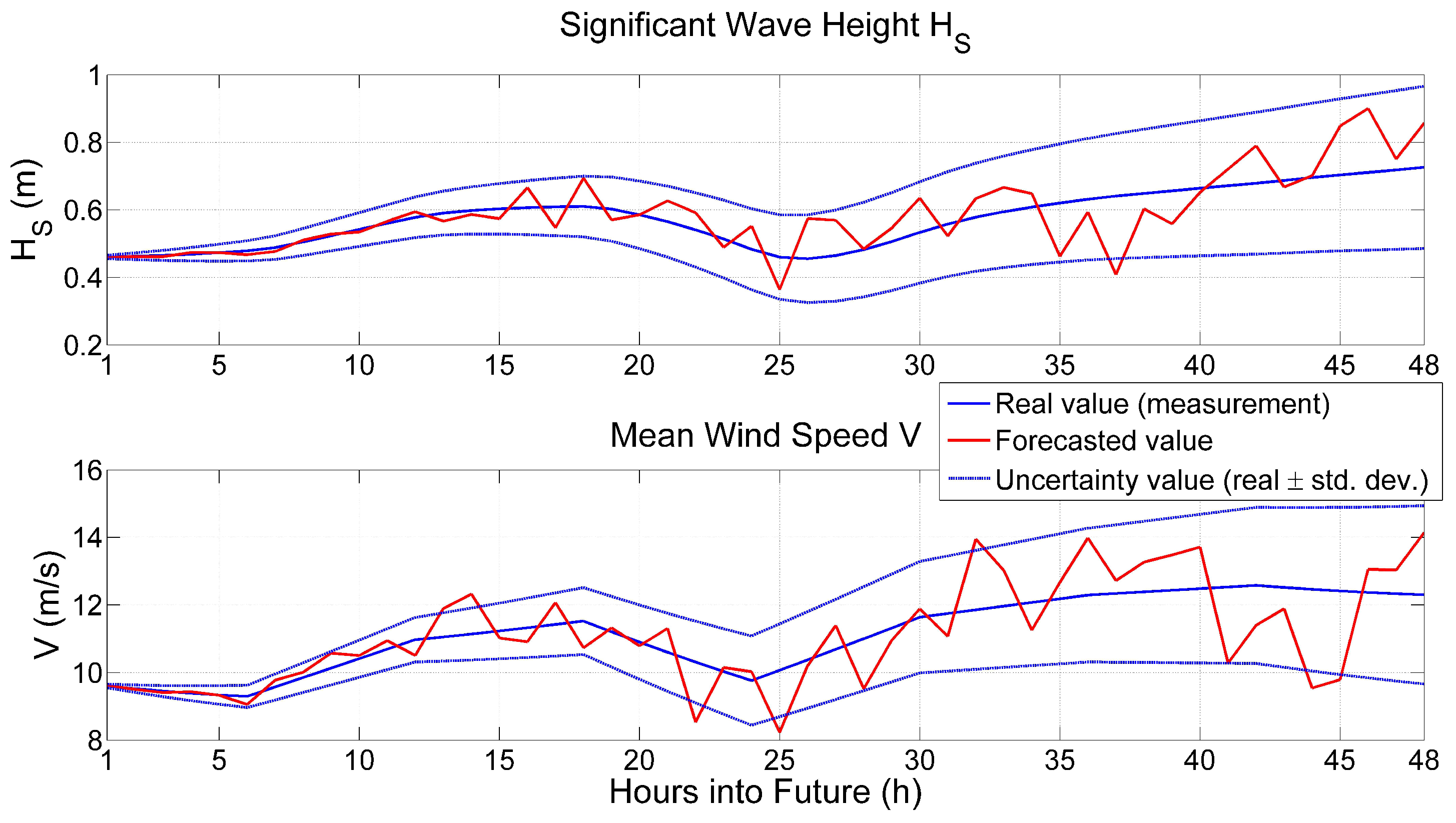
Figure 4.
Power curve of 6 MW reference offshore wind turbine [13].
Figure 4.
Power curve of 6 MW reference offshore wind turbine [13].
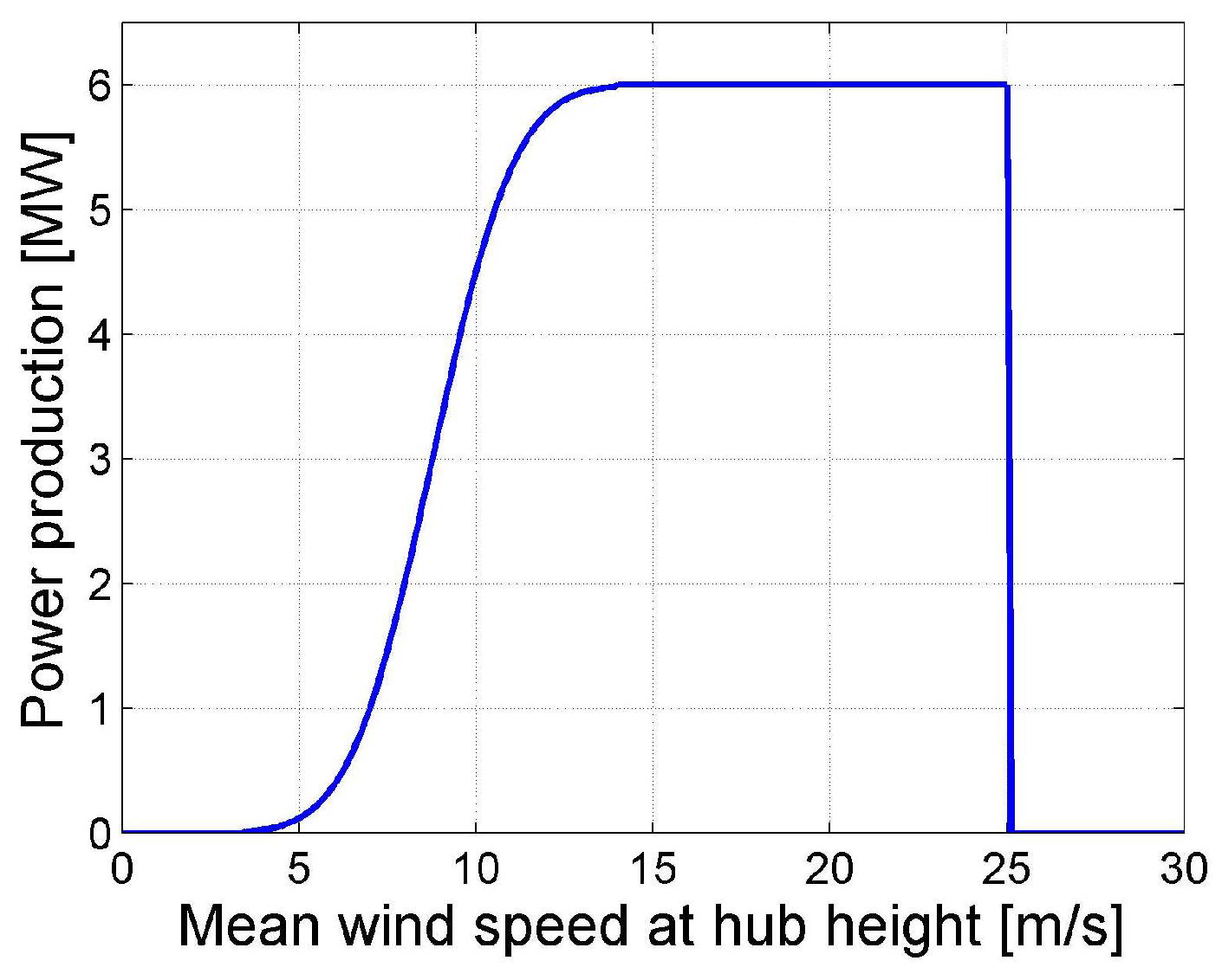
Figure 5.
Autocorrelation factor dependent on the forecast horizon for the mean wind speed and the significant wave height at the considered location. A polynomial fit with 7 degrees and a two term exponential function are fitted to the data.
Figure 5.
Autocorrelation factor dependent on the forecast horizon for the mean wind speed and the significant wave height at the considered location. A polynomial fit with 7 degrees and a two term exponential function are fitted to the data.

Figure 6.
Considered components of the 6 MW reference wind turbine for maintenance study. LSS: low speed shaft; and HSS: high speed shaft [13].
Figure 6.
Considered components of the 6 MW reference wind turbine for maintenance study. LSS: low speed shaft; and HSS: high speed shaft [13].
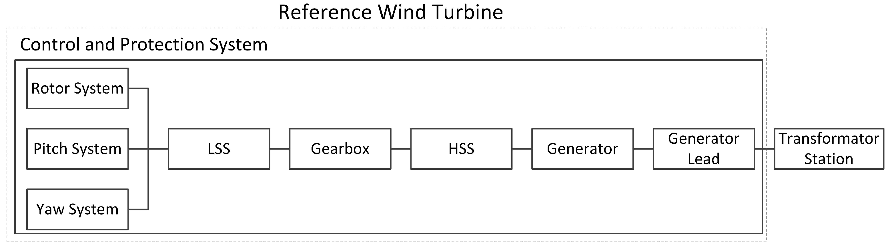
Figure 7.
Impact of weather forecast uncertainty on total maintenance expenses of the considered wind turbine farm during a lifetime of 20 years. WF: weather forecast; unc.: uncertainty; CM: condition monitoring; and regular: regular inspections every year.
Figure 7.
Impact of weather forecast uncertainty on total maintenance expenses of the considered wind turbine farm during a lifetime of 20 years. WF: weather forecast; unc.: uncertainty; CM: condition monitoring; and regular: regular inspections every year.
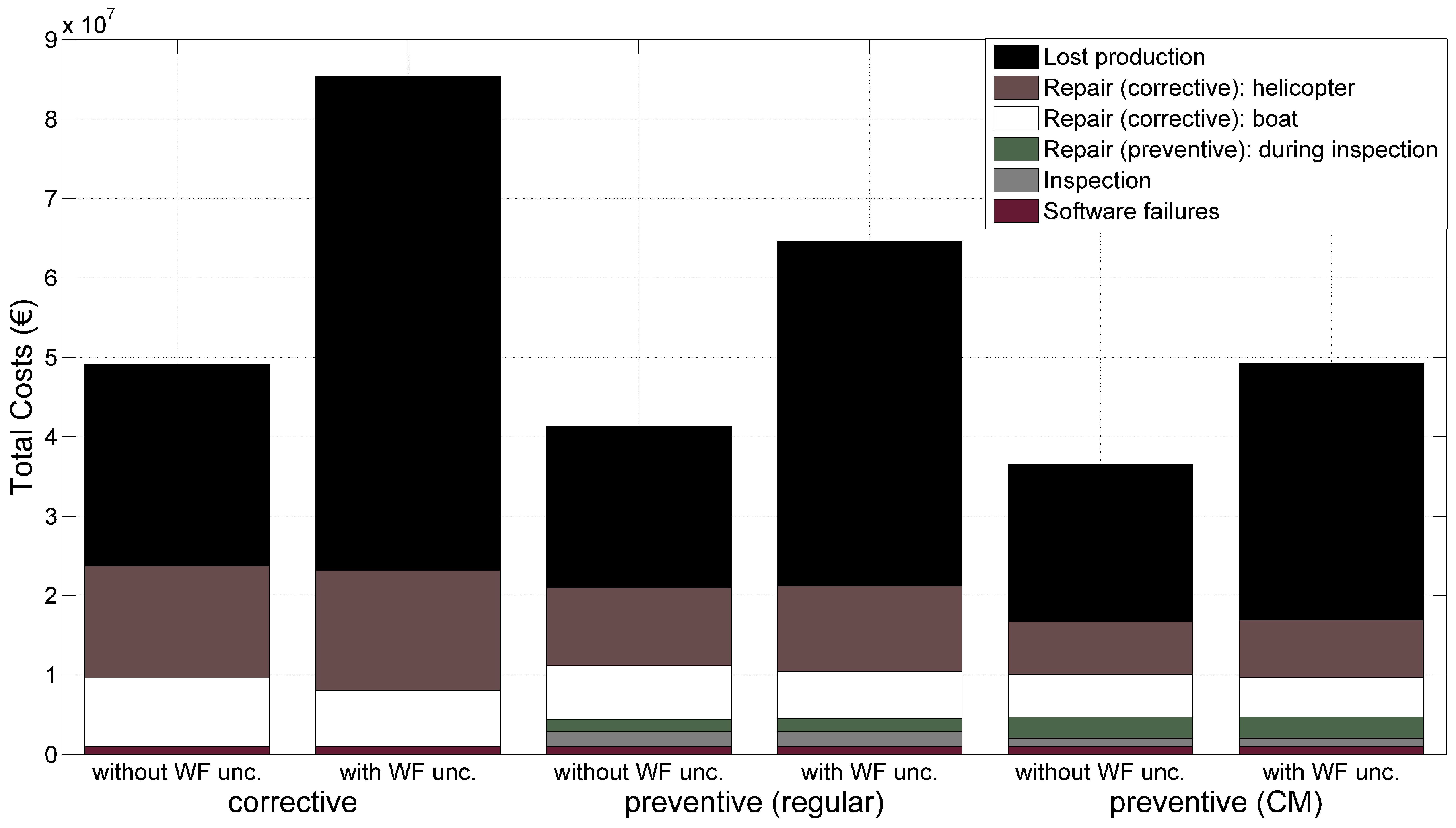
Figure 8.
Impact of weather forecast quality on total maintenance expenses of the considered wind turbine farm during a lifetime of 20 years. Bad weather forecast based on 120% uncertainties of the normal weather forecast and good weather forecast is equal to 80% of normal weather forecast uncertainties.
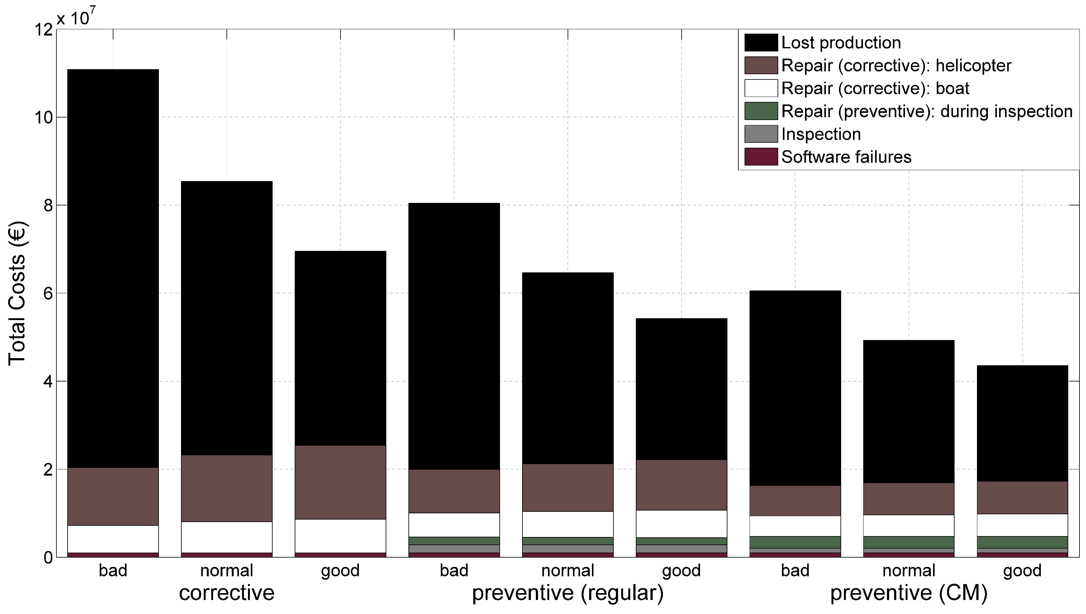
Figure 9.
Impact of value (models access uncertainty based on uncertain operational range of helicopter and boat) on total maintenance expenses of the considered wind turbine farm during a lifetime of 20 years.
Figure 9.
Impact of value (models access uncertainty based on uncertain operational range of helicopter and boat) on total maintenance expenses of the considered wind turbine farm during a lifetime of 20 years.

Figure 10.
Impact of value (models repair time uncertainty on the site) on total maintenance expenses of the considered wind turbine farm during a lifetime of 20 years.
Figure 10.
Impact of value (models repair time uncertainty on the site) on total maintenance expenses of the considered wind turbine farm during a lifetime of 20 years.

Figure 11.
Impact of all uncertainty sources value (models repair time uncertainty on the site) on total maintenance expenses of the considered wind turbine farm during a lifetime of 20 years. : 0.05; : 0.07.
Figure 11.
Impact of all uncertainty sources value (models repair time uncertainty on the site) on total maintenance expenses of the considered wind turbine farm during a lifetime of 20 years. : 0.05; : 0.07.

Table 1.
Weather forecast uncertainty values for wind speed and significant wave height. Time t is considered in hours. std.: Standard; and Sig.: Significant.
Table 1.
Weather forecast uncertainty values for wind speed and significant wave height. Time t is considered in hours. std.: Standard; and Sig.: Significant.
| Description | Forecast Term | |
|---|---|---|
| Mean Value | Std. Deviation | |
| Wind speed (m/s) | 0 | 0.055·t |
| Sig. wave height (m) | 0 | 0.005·t |
Table 2.
Considered damage parameters for different mechanical components of a wind turbine. Taken from [13]. Dam.: damage; exp.: exponent; Geom.: geometry; and COV: coefficient of variation.
Table 2.
Considered damage parameters for different mechanical components of a wind turbine. Taken from [13]. Dam.: damage; exp.: exponent; Geom.: geometry; and COV: coefficient of variation.
| Component | Dam. Exp. | Geom. Factor | Dam. Coefficient C | Proportionality Factor | ||
|---|---|---|---|---|---|---|
| m | Mean | COV | Mean | COV | ||
| Rotor system | 2 | 1 | 1.16 × 10 | 0.2 | 9.2 | 0.1 |
| Blade adjustment | 2.38 × 10 | 10 | ||||
| Gearbox | 1.65 × 10 | 8.6 | ||||
| Generator | 2.16 × 10 | 6 | ||||
| HSS | 1.07 × 10 | 3 | ||||
| LSS | 1.05 × 10 | 2.7 | ||||
| Yaw system | 1.57 × 10 | 8.2 | ||||
Table 3.
Considered failure rates taken from [13] for failures of electrical components and software.
Table 3.
Considered failure rates taken from [13] for failures of electrical components and software.
| Description | Mean Annual Failure Rates | Failure Type |
|---|---|---|
| Generator | 1.092 | electrical/software |
| Generator lead | 0.847 | electrical |
| Control and protection system turbine | 1.569 | electrical/software |
| Transformer station | 0.147 | electrical |
Table 4.
Considered probability of detection () values for inspection of mechanical components as well as parameters for preventive maintenance actions. Data taken from [13].
Table 4.
Considered probability of detection () values for inspection of mechanical components as well as parameters for preventive maintenance actions. Data taken from [13].
| Symbol | Meaning | Mean | COV | Distribution |
|---|---|---|---|---|
| Maximum probability of detection | 1 | - | Deterministic | |
| Expected smallest detectable damage | 0.4 | 0.1 | Normal | |
| Minimal damage for reparation/replacement | 0.3 | - | Deterministic | |
| Damage threshold for alarm of condition monitoring system | 0.8 | - | Deterministic |
Table 5.
Expected material and repair costs for different electrical and mechanical components of a 6 MW offshore wind turbine. Data taken from [13].
Table 5.
Expected material and repair costs for different electrical and mechanical components of a 6 MW offshore wind turbine. Data taken from [13].
| Description | Component Type | Expected Repair Costs (€) |
|---|---|---|
| Rotor system | mechanical | 4250 |
| Blade adjustment | mechanical | 4770 |
| Gearbox | mechanical | 5000 |
| Generator | mechanical/electrical | 7000 |
| Generator lead/cables | electrical | 9860 |
| HSS part | mechanical | 6530 |
| LSS part | mechanical | 6530 |
| Yaw system | mechanical | 8380 |
| Control and protection system turbine | electrical | 4400 |
| Transformer station | electrical | 14,520 |
Table 6.
Stochastic model representing the repair durations (in days) on the device for different mechanical and electrical failures. Data is adapted from [7,13,31,38].
| Description | Days Needed on Site for Repair | |
|---|---|---|
| Mean | COV | |
| Rotor system | 4 | 0.5 |
| Blade adjustment | 2 | |
| Gearbox | 3 | |
| Generator | 3 | |
| Generator lead | 2 | |
| HSS part | 3 | |
| LSS part | 3 | |
| Yaw system | 3 | |
| Control and protection system turbine | 2 | |
| Transformer station | 3 | |
Table 7.
Inspection and transportation costs as well as considered interest rate. Taken from [13].
Table 7.
Inspection and transportation costs as well as considered interest rate. Taken from [13].
| Description | Costs (€) | Rate (%) |
|---|---|---|
| Labor costs per day | 3600€ | - |
| Inspection (material) costs per component | 1000€ | - |
| Transportation cost by boat | 5000€ | - |
| Transportation cost by helicopter | 10,000€ | - |
| Interest rate r | - | 5% |
Table 8.
Expected values for availability (time- and power-based), total maintenance expenses in €/KWh and in percentages of the electricity prize (=0.08 €/KWh) as well as the COV of the expected costs in Figure 7.
Table 8.
Expected values for availability (time- and power-based), total maintenance expenses in €/KWh and in percentages of the electricity prize (=0.08 €/KWh) as well as the COV of the expected costs in Figure 7.
| Maintenance Strategy | Corrective | Preventive (Regular) | Preventive (CM) | |||
|---|---|---|---|---|---|---|
| Weather Forecast | Perfect | Imperfect | Perfect | Imperfect | Perfect | Imperfect |
| Availability (time-based) | 0.916 | 0.761 | 0.930 | 0.834 | 0.920 | 0.870 |
| Availability (power-based) | 0.903 | 0.744 | 0.922 | 0.823 | 0.925 | 0.871 |
| O&M expenses/KWh (€/KWh) | 0.016 | 0.034 | 0.014 | 0.023 | 0.012 | 0.017 |
| O&M expenses/KWh (%) | 20.5 | 42.3 | 16.7 | 29.3 | 14.9 | 21.3 |
| COV total maintenance expenses (-) | 0.063 | 0.211 | 0.065 | 0.243 | 0.068 | 0.246 |
Table 9.
Total maintenance expenses, availability, O&M expenses per produced KWh and COV of expected maintenance costs ratio between simulations with and without uncertainty (weather forecast, repair time and operational range of boat/helicopter) consideration. reg.: regular.
Table 9.
Total maintenance expenses, availability, O&M expenses per produced KWh and COV of expected maintenance costs ratio between simulations with and without uncertainty (weather forecast, repair time and operational range of boat/helicopter) consideration. reg.: regular.
| Description | Maintenance Strategy | ||
|---|---|---|---|
| Corrective | Preventive (Reg.) | Preventive (CM) | |
| Total maintenance expenses ratio | 2.309 | 2.378 | 1.721 |
| Availability ratio (time-based) | 0.690 | 0.746 | 0.884 |
| Availability ratio (power-based) | 0.681 | 0.734 | 0.878 |
| O&M expenses/KWh ratio | 3.231 | 3.132 | 1.935 |
| COV total maintenance expenses ratio | 3.006 | 3.346 | 3.712 |
© 2017 by the authors. Licensee MDPI, Basel, Switzerland. This article is an open access article distributed under the terms and conditions of the Creative Commons Attribution (CC BY) license (http://creativecommons.org/licenses/by/4.0/).
Share and Cite
MDPI and ACS Style
Ambühl, S.; Dalsgaard Sørensen, J. Sensitivity of Risk-Based Maintenance Planning of Offshore Wind Turbine Farms. Energies 2017, 10, 505. https://doi.org/10.3390/en10040505
AMA Style
Ambühl S, Dalsgaard Sørensen J. Sensitivity of Risk-Based Maintenance Planning of Offshore Wind Turbine Farms. Energies. 2017; 10(4):505. https://doi.org/10.3390/en10040505
Chicago/Turabian StyleAmbühl, Simon, and John Dalsgaard Sørensen. 2017. "Sensitivity of Risk-Based Maintenance Planning of Offshore Wind Turbine Farms" Energies 10, no. 4: 505. https://doi.org/10.3390/en10040505
Note that from the first issue of 2016, this journal uses article numbers instead of page numbers. See further details here.