High Robustness Control for Robotic Wireless Power Transfer Systems with Multiple Uncertain Parameters Using a Virtual Buck Converter

School of Automation, Chongqing University, 174 Shazheng Street, Shapingba District, Chongqing 400030, China
*
Author to whom correspondence should be addressed.
Energies 2017, 10(4), 517; https://doi.org/10.3390/en10040517
Submission received: 10 February 2017
/
Revised: 5 April 2017
/
Accepted: 6 April 2017
/
Published: 11 April 2017
(This article belongs to the Section D: Energy Storage and Application)
Abstract
:Aiming at achieving high robustness performance in Wireless Power Transfer (WPT) systems for moving robot power supply, this paper proposes a H∞ robust control method with multiple parameters that vary randomly, including the mutual inductance, load parameter, and operating frequency. These uncertain parameters make the system control extremely difficult. A composite Upper Linear Fractional Transformation (LFT) method is proposed to deal with the system uncertainty, particularly for the mutual inductance detachment, which is very unique and important for WPT systems. A suboptimal H∞ controller design method is proposed based on Generalized State Space Averaging (GSSA) model in order to simplify the system structure. In controller implementation, a virtual buck converter for phase shifted regulation is proposed to replace real input buck converter. The proposed H∞ control method is easy to implement because only the output voltage of the WPT system needs to be sampled, and based on which a simple DSP control algorithm is developed. Simulation and experimental results have demonstrated that the proposed control method can achieve less than 15 ms response speed with 70% mutual inductance variation and 50% load variation tolerance respectively.
1. Introduction
Wireless Power Transfer (WPT) is a novel technology that can realize efficient energy transmission between two electrically isolated coils by high frequency magnetic coupling. As the magnetic field is used as energy transmission media, the process of energy transmission is unaffected by water or dirt and is intrinsically safe for human beings and animals [1,2]. In recent years, WPT technology has found more and more applications in mobile robots and microrobots used in the human body [3,4,5].
A robot power supply WPT system is characterized by loose magnetic field coupling and resonant operation, which results in system parameter uncertainty. Many circuit parameters such as the coil inductances, coupling coefficients, and reflecting impedance may vary dynamically during operation. Firstly, the coupling variation when the robot is moving may lead to significant variation in the mutual inductances. Due to relatively large movements between the primary and secondary sides, the mutual inductance may randomly drift away from the designed value [6,7,8]. Secondly, the load may vary under different output power requirements for a robot’s different action requirements. The third uncertain parameter is the operating frequency. Due to soft switching requirements, the switching frequency should dynamically change according to the inherent frequency variation of the resonant tank. It should be noted that the inherent frequency is also an uncertain parameter affected by the mutu1al inductance, the load, and other parameters [9]. These multiple uncertain parameters will greatly increase the complexity of the system behaviors. Moreover, due to existence of the resonant tank, the WPT system often exhibits high system orders. For example, in a composite resonant type system such as LCL (L-inductor, C-capacitor, L-inductor), the system order can reach 7 or even higher [10]. The multiple uncertain parameters, high system order, and switching nonlinearity will make the system modeling and control extremely difficult [10]. In short, these dynamical variations of system parameters will bring system with uncertainty and influence system performance. Therefore, it is necessary to put forward a robust control method for robot wireless power transfer systems.
The classical control of a WPT system is mainly focused on a single objective such as tuning point control and power flow control. Hysteretic Bang-Bang control and PID (Proportion Integration Differentiation) control are two typical control methods. Although these control methods are easy to implement [2,11,12,13], they normally cannot fulfill multi-objective and robust performance requirements. As a result, more attention is being paid to advanced control methods. Recent research work can be categorized into sliding mode control [14], fuzzy control [15], optimal PID control [16] and robust control method [10]. For sliding mode control, an adaptive sliding-mode control method is proposed for WPT system [14]. This method can realize output power control for multiple users system, but prior knowledge is required for sliding mode surface design. For fuzzy control, a full directional tuning control method by using a fuzzy logic control method is proposed [15]. The logic control is used to determine the tuning step-size to overcome the chattering effects of using a fixed tuning step-size. For PID control, aiming at the PID tuning problem, a derivative-free optimization technique based on a genetic algorithm is proposed [16]. The PID parameters can be optimized by this offline calculation algorithm. The main feature of the Bang-Bang, PID, and fuzzy and sliding mode control methods is the independence of the system model, therefore avoiding the model complexity problem. However, these control methods are single-objective control methods and the robustness uncertain parameters variation cannot be taken into account. When the system parameters drift randomly, these controllers may not achieve good control performance. Furthermore, since the controller design process is independent of the system model, a trial-error method is often used to determine an optimal set of controller parameters, especially for a PID controller. Robust control is another method based on comprehensive system modeling. All system parameters including the uncertain parameters are embedded in the system model. A distinguishing feature of the robust control method is its multi-objective control characteristics. It can guarantee the output stability, reference tracking, anti-perturbation performance, as well as control energy optimization at the same time. It is relatively easy to design the controller by following a routine design process.
The current research on robust control of WPT is still at its initial stage. In 2013, Li et al. proposed a μ-synthesis robust control method for WPT systems [10]. In the paper, only frequency uncertainty was taken into account, but it is difficult for the mutual inductance to be separated from the system model because this parameter appears in cross-coupling differential equations. Furthermore, traditional μ-synthesis control methods cannot be used in a system with multiple uncertain parameters including mutual inductance because these multiple uncertain parameters will increase the order of the uncertainty block and it is very difficult for the D-K iteration in the μ-synthesis control to converge. In addition, a real buck converter may need to be added to regulate the primary DC input [10], which increases the system complexity and slows down the system response speed.
Aiming at the robust control and anti-perturbation performance improvement for robot power supply, this paper proposes a novel H∞ robust control method for the WPT system with multiple uncertain parameters. Firstly, instead of using a real power converter, a virtual buck converter is developed using a phase-shifted inverter to regulate the equivalent DC input voltage. Secondly, a Generalized State Space Averaging (GSSA) model is established based on a differential system modeling. Thirdly, the paper proposes a multiple uncertain parameters modeling method by upper Linear Fractional Transformations (LFT). Based on the new model, the design method of a H∞ suboptimal controller is proposed. The controller stability and performance based on Structure Singular Value (SSV) are analyzed.
The main achievement of this paper is finding a robust control method which can take uncertain coupling coefficient into robust control. Traditionally, it’s very difficult to detach this uncertain parameter from the system model due to the complexity of the cross coupling equations. The other achievement is finding a virtual buck converter to implement robust control for phase-shift converter, which can be applied to any other system.
2. Phase-Shifted Control and Virtual Buck Converter
2.1. Phase-Shifted Control
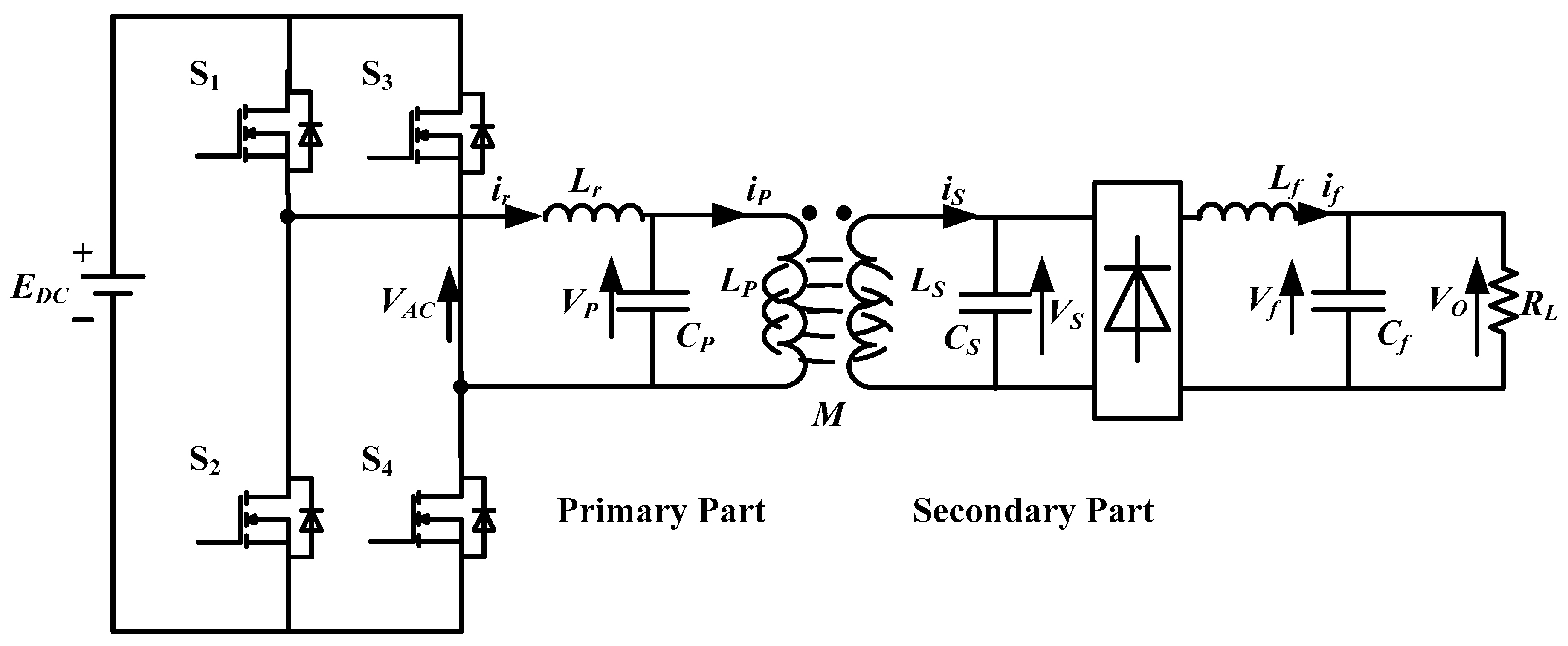
LCL type WPT system is a composite resonant system which exhibits great filtering capability. This topology is widely used in the mobile device charging applications [9,17,18]. Figure 1 shows a typical LCL-P topology of a WPT system.
The whole system can be divided into two parts, the primary part and the secondary part. The primary part comprises a phase-shifted inverter consisting of four switching devices (S1–S4) which convert DC input into high frequency AC output and a LCL composite resonant tank consisting of Lr, CP and LP. A DC voltage input is transformed into phase-shifted voltage by the phase shifted inverter and injected into the LCL resonant tank. With the aid of the LCL filtering capability, a sinusoidal current will appear in magnetic excitation coil (LP). The secondary part comprises a parallel resonant tank (LS, CS), a rectifier and a filter (Lf, Cf). The parallel resonant tank is used to boost the power transfer capability. The rectifier with the filter is used to produce a stable DC output for the load.
With the phase-shifted inverter, the output power can be regulated by a phase-shifted angle α. Figure 2 shows the phase-shifted control method. The waveforms from top to bottom in the figure are the driving signals of S1–S4, the phase-shifted voltage VAC, and primary coil current iP respectively. The lagging angle between two bridge arms is the phase-shifted angle α. The two switching devices on the same bridge arm such as (S1, S2) and (S3, S4) should be conducted complementarily to prevent short of EDC.
2.2. Virtual Buck Converter
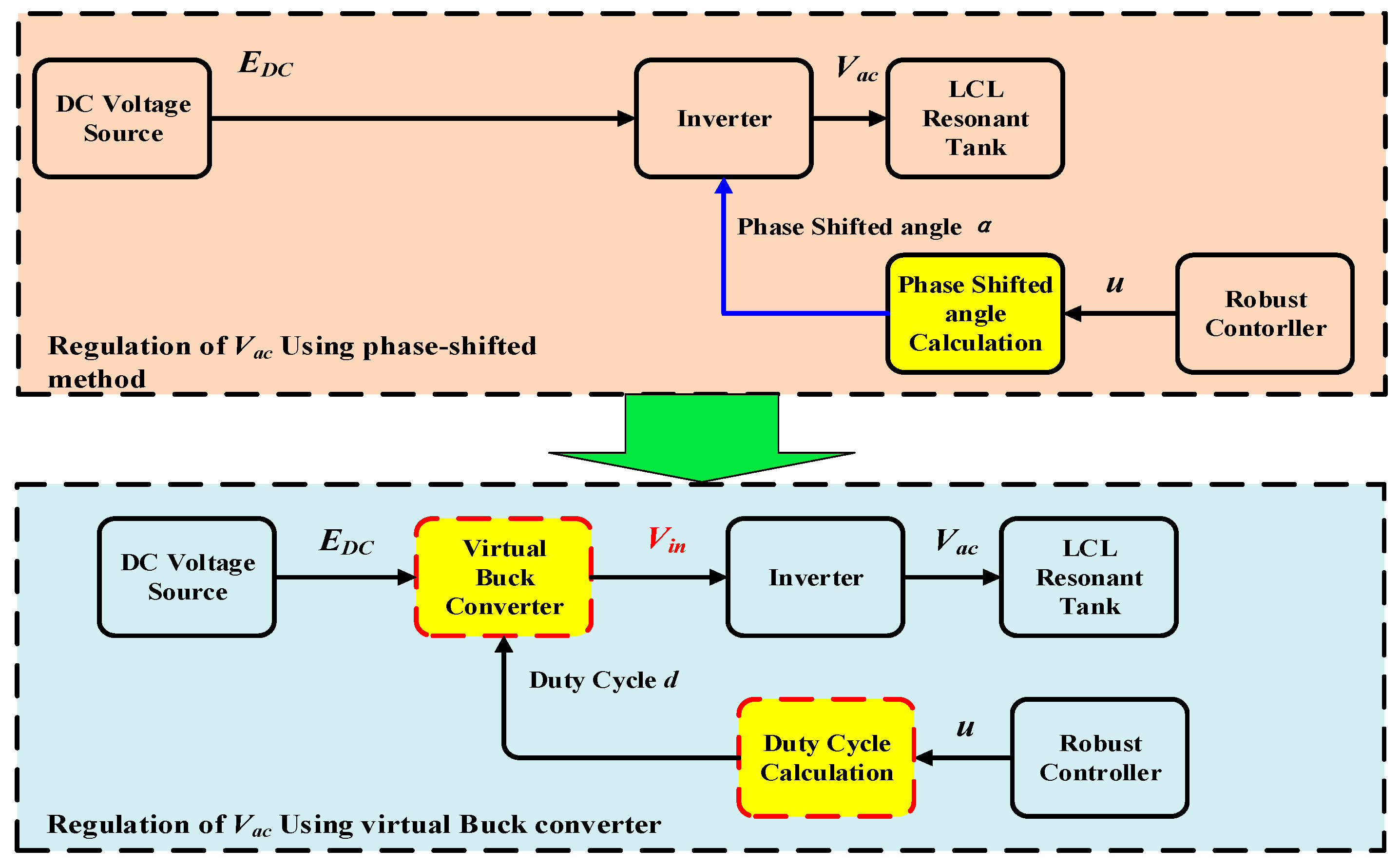
In the conventional robust controller design for a WPT system, a buck converter is often added in front of the primary inverter to obtain a regulated DC-DC input [10]. The buck converter will cause additional power losses and make whole system bulky. Therefore, in this paper, the phase-shifted regulation method is utilized as a good alternative. However, since the robust control is only applicable for variable DC input system, the phase-shifted method cannot be directly used in the robust control system. This paper proposes a virtual buck converter scheme to obtain an equivalent variable input for the phase-shifted regulation system. There is an assumption that the phase-shifted voltage Vac can be approximated by its fundamental harmonics Vac. Due to the great filtering capability of the LCL resonant tank, this assumption holds. Based on this assumption, the virtual buck converter scheme can be shown in Figure 3.
The upper one in Figure 3 is the phase-shifted method. The lower one is its equivalent regulation method using a virtual buck converter. In the real system, the inverter is controlled by a phase-shifted angle α to produce the required Vac, but it cannot be directly used for robust control as an adjustable DC input is required. In this paper, the regulation of Vac using phase-shifted regulation is mapped to an equivalent regulation of Vac using a virtual buck converter. As a result, a virtual adjustable DC input Vin can be obtained for robust controller design.
For the regulation of Vac using phase-shifted method, the RMS value of Vac can be given by:
For the equivalent regulation of Vac using a virtual buck converter, due to the inverter operating under non-phase-shifted mode, the phase-shifted angle α should be π. Thus, the RMS value of Vac can be given by:
The transfer function of the duty cycle calculation block is designed as:
The transfer function of the virtual buck converter is:
Therefore, the controller output u would equal the virtual regulation input Vin. In order to acquire same Vac, (1) and (2) should be equal and the phase-shifted angle α can be obtained by:
With (5), the controller output u can be mapped back to the real system to produce a phase-shifted angle α.
3. GSSA Modeling
Due to the existence of switching nonlinearity, classical linear modeling methods cannot be directly used. The GSSA modeling method is a nonlinear modeling method, which can be used to solve the modeling problem for power electronics systems. This paper utilizes the GSSA modeling method to transform the nonlinear model in the time domain to a linear state space model in the frequency domain. The first step of GSSA modeling is to set up the differential model based on the equivalent system model, which is shown in Figure 4.
According to the equivalent circuit, the differential model of the LCL system can be obtained as:
where RLr, RLp and RLs are the equivalent series resistances of the inductances Lr, LP and LS, respectively. The fp(t) and fs(t) are switching functions which have a 180° phase difference. They are given by:
The GSSA method is based on the concept that a signal x(τ) can be approximated on the interval to arbitrary accuracy with a Fourier series expansion where ω = 2π/T = 2πf. T is the chosen period of fundamental harmonic. The time-dependent complex Fourier coefficient is the index-n coefficient, given by The key point of the GSSA method is to substitute the complex Fourier coefficient for the time domain signals x(t). In the WPT system, for the state variables exhibiting predominantly sinusoidal-type behavior, they can be replaced by their index-one coefficients (). For the state variables exhibiting predominantly constant (or slowly varying) behavior, they can be replaced by their index-zero coefficients () [19].
The GSSA model of the LCL type WPT system can be obtained as:
where .
However, since all are complex Fourier coefficients, it’s not convenient for controller design. Therefore, these complex state variables are detached to variables of real part and variables of imaginary part respectively, which can be shown as:
The output voltage Vo is set as the output y which is equal to Vf. Then the GSSA model is obtained as:
where .
4. Multiple Uncertain Parameters Modeling
The mutual inductance M, running frequency ω and load parameter RL are three primary uncertain parameters. They are defined as , and , respectively. , and are the nominal values of ω, RL and M while , and represent the maximum variation range of these parameters. The variables , and are normalized uncertain variables in the interval [−1, 1].
Furthermore, these uncertain parameters can be expressed using upper LFT method. LFT method is utilized to detach the uncertain part from the system model:
The block diagrams of these LFTs can be shown in Figure 5:
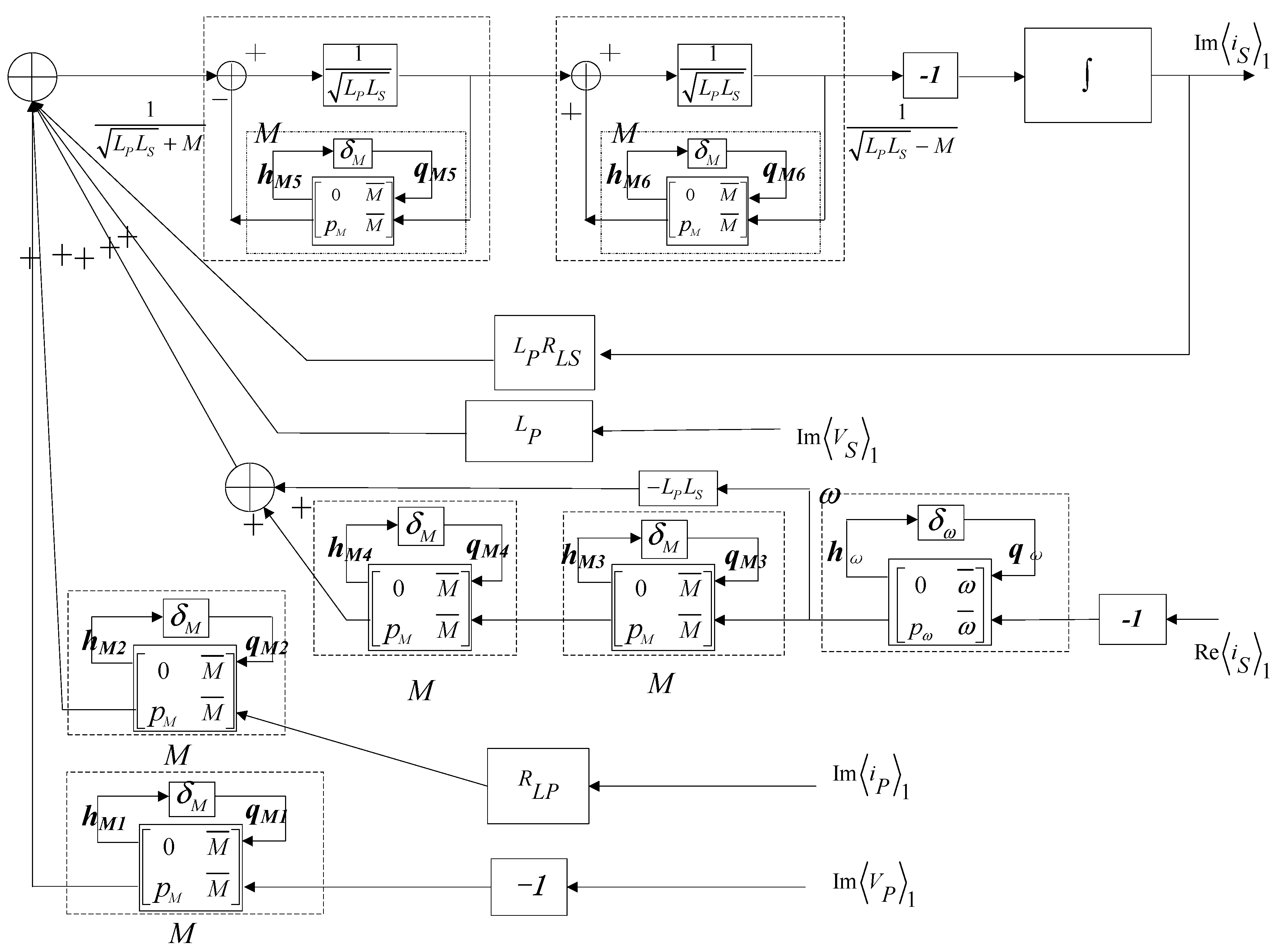
By substituting these LFT of uncertain parameters into system GSSA model given in (10), and extracting the uncertainty coefficients from the GSSA model, the uncertain part can be detached from the system model by a special composite upper LFT method proposed in this paper. The detailed procedure of this process is given in Appendix A. The system model after uncertain part detachment is shown in Figure 6.
In Figure 6, the Gnom block is the system model with all certain parameters and the Δ block is the uncertain model part including all normalized uncertain variables. The perturbed input h and perturbed output q are defined as:
The state space representation of Gnom is given as:
where is the coefficients matrix of the Gnom.
5. H∞ Suboptimal Controller Design
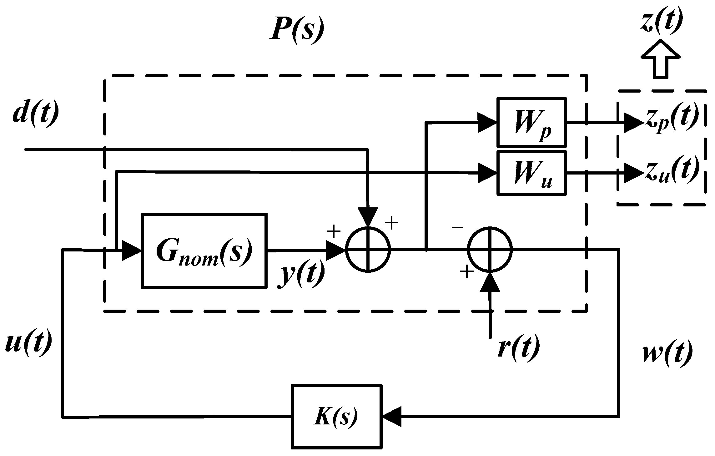
In order to realize multi-objective control, it is necessary to set a cost function to take into account the performance requirements including reference tracking, anti-perturbation and control energy limitation. Based on these requirements, the system structure can be established by using mixed sensitivity optimization design, which is shown in Figure 7.
Here Gnom(s) is the nominal system of G(s), which denotes the system without uncertainty. K(s) is the transfer function of the output feedback controller. Wp(s) and Wu(s) are a performance weighting function and control weighting function, respectively. Signals d(t), w(t) and u(t) are perturbation, measured error and control input. The two weighted outputs zp(t) and zu(t) are performance indexes output which can be grouped into a performance output vector z(t), which denotes system performance requirements. Thus the transfer function matrix from d(t) to z(t) can be obtained as:
where S(s) is the sensitivity function which combines multiple robust control objectives and R(s) is the control sensitivity function. The mixed sensitivity H∞ suboptimal control method is to find a controller K(s) which can stabilize the closed-loop system in Figure 6. That is, for a given small scalar γ > 0, the controller K(s) should satisfy:
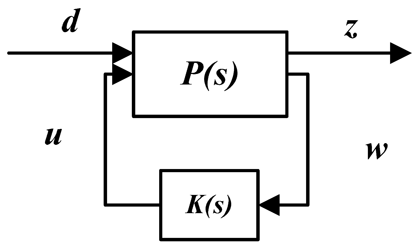
This cost function in (18) combines the design objectives of reference tracking, anti-perturbation, less control energy and robust stabilization together. With the cost function, the H∞ robust control system will be as shown in Figure 8.
where P(s) is called the generalized plant model which includes the nominal model Gnom and weighting function Wp and Wu. It can be given by:
where is the augmented coefficient matrix. The cost function in (16) can be redefined as: Given a positive number γ, to find a stabilizing controller K(s) satisfying H∞-norm of the closed-loop transfer function less than γ. It can be given by:
where .
In the controller design stage, since multiple uncertain parameters are involved, the dimension of the uncertainty block will be 35 × 35 (corresponding to δω, δRL and δm). As far as the μ-synthesis control method is concerned, the 35 × 35 uncertainty block will cause the D-K iteration algorithm to fail to converge. Thus the μ-synthesis control method cannot be applied. However, the H∞ suboptimal control is a signal-based control algorithm utilizing the H∞ norm. This control method can obtain more freedom in designing high order robust controller and it can also obtain good robust performance and robust stability against system perturbations.
In selecting the weighting function, normally the performance weighting function Wp(s) is designed as a high gain low-pass filter to emphasize the tracking accuracy at low frequencies. Hence, the weighting function Wp(s) is selected in the form of first-order transfer function as:
The control weighting function Wu(s) is usually chosen as a high-pass filter or just a scalar to limit the control energy and actuator saturation [20].
After uncertainty modeling and weighting functions selection, the suboptimal H∞ controller design can be realized with aid of the Robust Control Toolbox of MATLAB. Based on the generalized plant model P(s), the robust controller K(s) can be directly obtained using the hinfsyn function. The form of function call is hinfsyn (P, nmeas, ncon, gmin, gmax, tol), where P denotes P(s) model, nmeas and nmeas are the numbers of output and control input. Parameters gmin, gmax and tol are the lower and upper bound and tolerance of γ, respectively. The order of the obtained controller is 13. In order to make it easy for implementation, the controller order needs to be reduced. Based the optimal Hankel-norm approximation of a system matrix, the controller order is reduced to 3 using hankmr function. The form of function call is hankmr (sys, sig, k, opt), where parameter sys and sig denotes system model. Parameter k denotes the reduced order. Furthermore, in order to make the controller suitable for digital CPU implementation such as DSP, the discretization of controller is carried out using the samhld function. The form of function call is samhld (sys, T), where parameter sys denotes system model and T is the discretization sampling period. In summary, the whole robust controller design procedure can be as represented by Figure 9.
6. Analysis of H∞ Controller
In order to analyze the performance and stability of robust controller, a demo system is set up. To stay consistent, all parameters in controller computation, analysis, simulation and experiments are kept the same, and they are listed in Table 1 and Table 2.
The weighting function is given by and the control weighting function is selected as . The upper bound of performance index γ is set at 0.5. Then the obtained controller K(s) is given by:
The achievable minimum value of γ for is 0.0039. This demonstrates that this closed-loop system has a good robust performance.
In order to gain a deep insight of the performance of the H∞ suboptimal controller K(s), the structured singular value analysis (μ analysis) method can be used to evaluate the robust stability and robust performance of the closed-loop system.
Based on the generalized plant model P(s) (19) and the H∞ suboptimal controller K(s) in Section 5 a standard J-Δf configuration for μ analysis can be obtained as shown in Figure 10. In Figure 10, J(s) is the transfer function matrix obtained via the lower LFT technique, i.e., . The uncertainty block is given as and is the performance uncertainty block.
First, the robust stability analysis is given. It shows the controller ability to maintain system output stability on the condition of uncertain parameters variation. The upper and lower bounds of over a certain frequency range are shown in Figure 11.
Figure 11 shows that in the frequency interval [10−2 106] (rad/s), the peak value of μ is 0.936 which indicates < 1 is satisfied. It shows that the system stability can be maintained for all Δ satisfying ||Δ||∞ < 1/0.936. Hence, when the multiple uncertain parameters vary in the range given in Table 1, the robust stability can be guaranteed.
Secondly, the robust performance analysis is given. It shows that the ability of the controller to eliminate the perturbation from the uncertain parameters. Since the performance output z(t) in Figure 10 is a 2-dimensional vector, the performance uncertainty block ΔP is defined as a 1 × 2 full block. The total structured uncertainty block Δf is defined as:
The upper and lower bounds of over a certain frequency range are shown in Figure 12.
In Figure 12, the peak value of is equal to 0.871. It demonstrates that the closed-loop system achieves good robust performance for all Δ satisfying ||Δ||∞ < 1/0.871. Hence, the robust performance can be guaranteed when the perturbations from the uncertain parameters are within the range given in Table 1.
7. Simulation Results
In order to verify the H∞ control method, a simulation model is set up using Simulink as shown in Figure 13. In this model, to make the controller easy for implementation in digital processing unit, the discretized robust controller based on (22) is given by:
The output voltage Vo is compared with a reference voltage to produce error signal e. The discretized H∞ controller produces control output u based on the error signal e. The phase-shifted angle is calculated with u according to Equation (5).Then this angle is converted to the driving signal for the phase-shifted inverter.
In order to evaluate the dynamic performances of the closed-loop system with the H∞ controller, the ramp and step reference tracking, load perturbations tests were carried out.
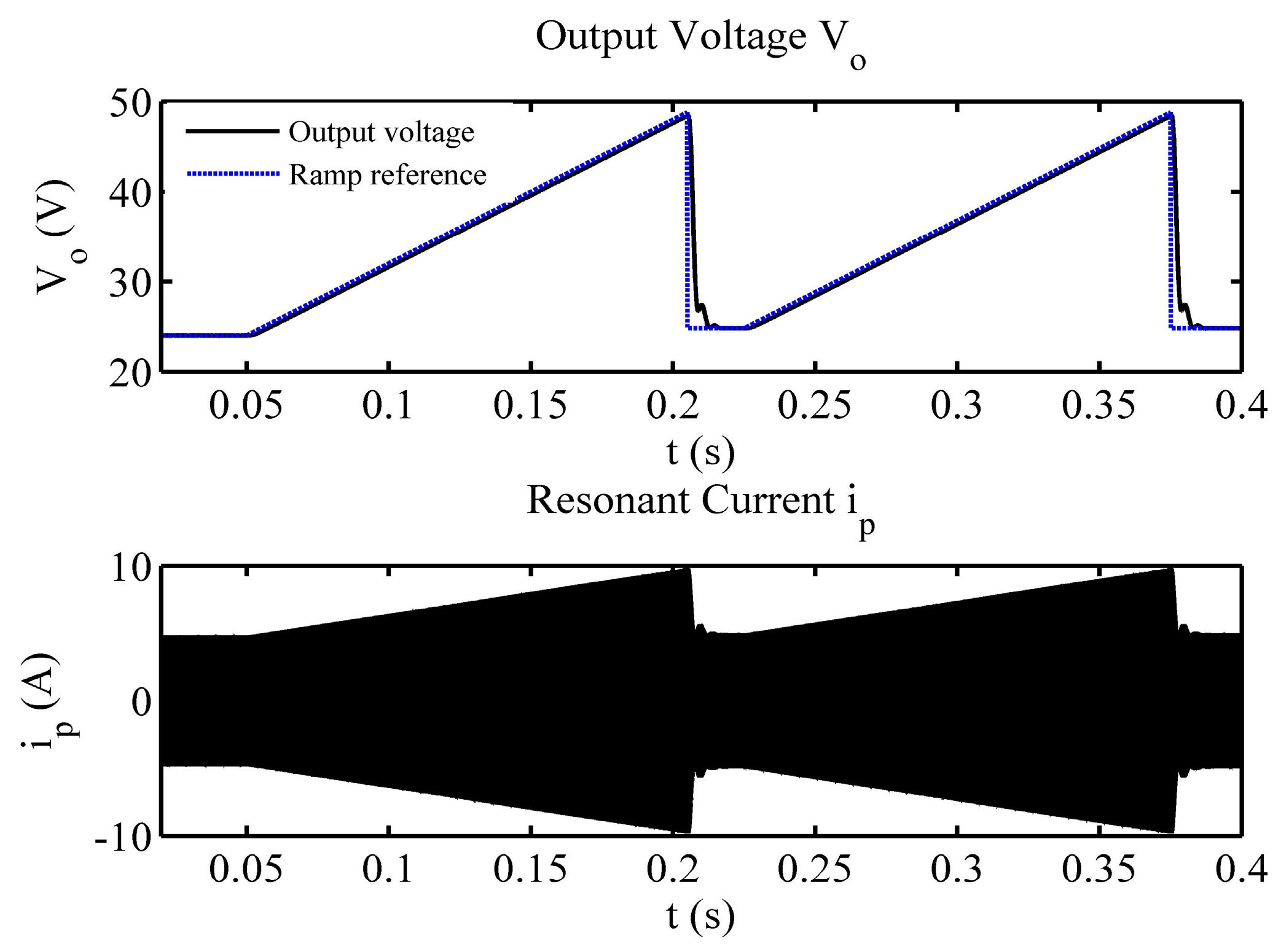
First, the simulation of the closed-loop system with a ramp reference was carried out and the reference was a ramp signal varied from 24 V to 48 V. The simulation result is shown in Figure 14.
Figure 14 shows that the output voltage Vo was able to track the ramp reference signal rapidly while the resonant current ip changes from 4.8 A to 9.8 A. It denotes the controller has a good tracking ability for continuous varying reference. Secondly, the reference jump test was carried out to show the performance of the closed-loop system. The reference jumps was designed in the sequence of 32 V–48 V–32 V. The simulation result is shown in Figure 15.
Figure 15 shows that with the H∞ control, the output voltage Vo can track the reference variation (32 V–48 V and 48 V–32 V) within 10 ms and there are no overshoot in the adjusting process. Thus, based on the results shown in Figure 14 and Figure 15, it can be concluded that closed-loop system has achieved the fast and accurate dynamic tracking performance with the H∞ controller.
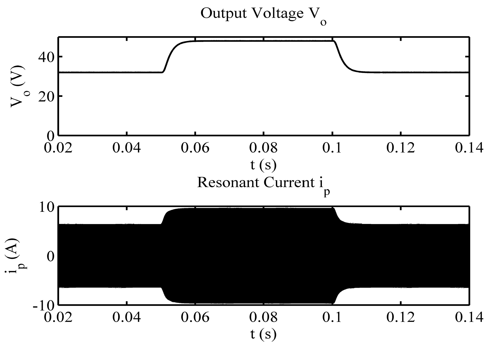
Thirdly, to verify the robustness of the closed-loop system under load perturbation, simulation results were obtained on the condition of load resistance variation. The control aim is to maintain the output voltage stable at 48 V. The load resistance variation is set in the sequence of 50 Ω–100 Ω–50 Ω. The simulation result can be shown in Figure 16.
Figure 16 shows that for the first load jump from 50 Ω to 100 Ω, it takes about 8 ms to complete the control regulation and there is a 12 V voltage overshoot in the process. For the second load jump from 100 Ω to 50 Ω, it takes 10 ms to complete control regulation and there is 8 V overshoot. The simulation results show the controller has a good anti-perturbation ability for load variation.
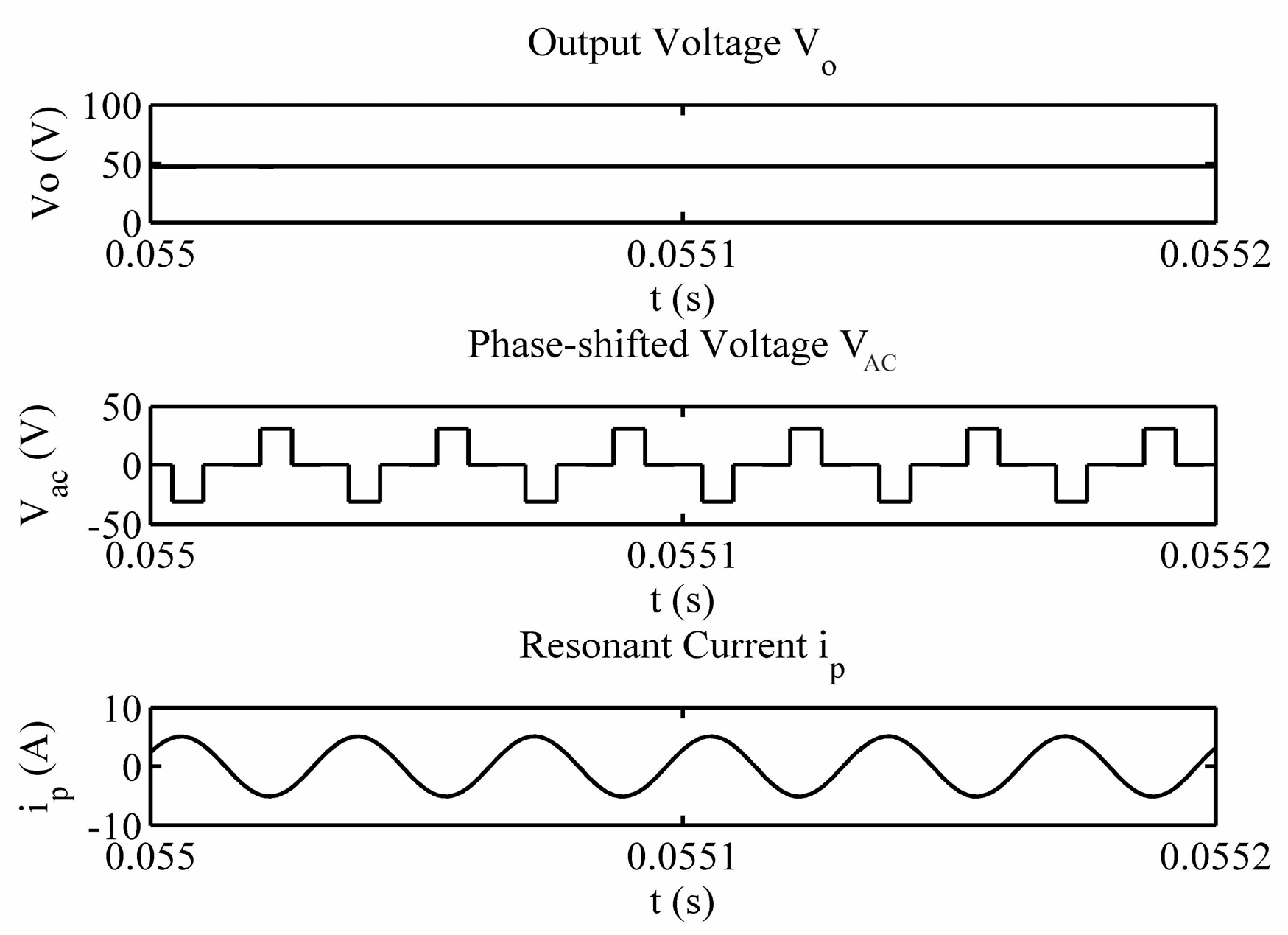
In Figure 17 and Figure 18, the zoomed waveforms of the output voltage Vo, phase-shifted voltage VAC, and resonant current iP in the steady state under different load conditions. Regardless of 50 Ω or 100 Ω load conditions, the output voltage Vo, the phase-shifted voltage VAC and the resonant current iP are stable and there is no ripple on the output voltage and phase-shifted voltage. Moreover, there is also no distortion on the resonant current. It shows that the controller also has a good performance in the system steady state.
8. Experimental Results
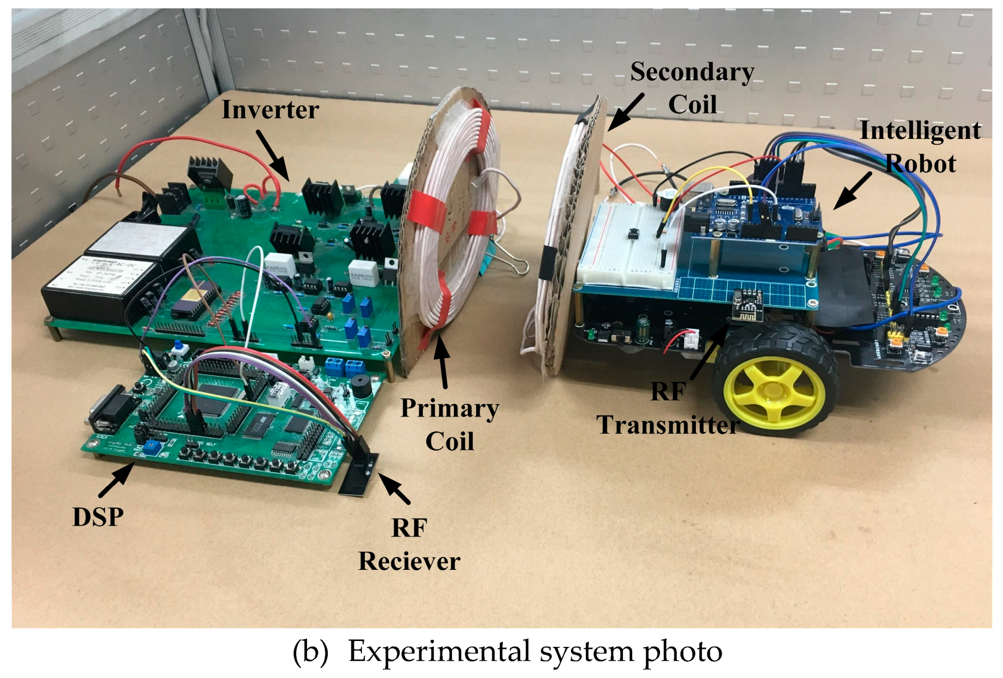
An experimental system was set up for verification. The system structure and a photo can be seen in Figure 19.
In the experimental system, an IRF 540 MOSFET was used for the switching components S1–S4. The primary and secondary coils (LP and LS) were made by Litz wire with 24 turns and 15 cm diameter. RF-link was built up by nRF2401 RF module working at 2.4 GHz to realize information exchange.
The discretized H∞ controller in (24) is implemented on a TMS320LF2407 DSP microcontroller. The output voltage Vo is sampled and sent to the primary side by using the RF-link. According to the output voltage, the DSP will calculate the control output and corresponding phase-shifted angle. The phased-shifted pulses are produced by the gate drive block to the inverter. A ZCS detection block is used to realize zero current switching (ZCS). However, due to the phase-shifted requirement, the ZCS operation cannot be guaranteed for all switching process.
For verification, several experiments were carried out. First, the test of ramp reference tracking was implemented. The response of the closed-loop system with ramp reference starting from 24 V to 48 V is shown in Figure 20. The output voltage Vo can track the ramp reference smoothly with the peak value of the resonant current ip varying from 5 A to 8.5 A.
Firstly, his test of reference jump was carried out. The response of voltage reference jumping from 32 V to 48 V and then returning to 32 V is shown in Figure 21. It takes 12 ms and 11 ms to complete the control regulation for the first and second reference jump, respectively. There are no significant overshoots and ripples on either output voltage Vo or resonant current ip. From Figure 21, it can be concluded that the H∞ controller can achieve good dynamic tracking performance.
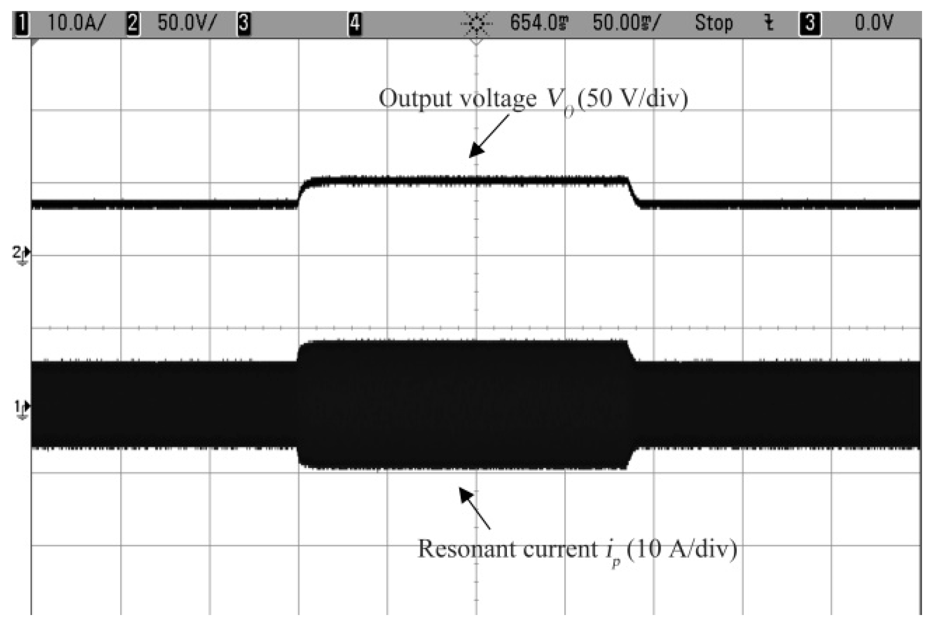
Secondly, the test of load perturbation was carried out. The response of load resistance jumping from 50 Ω to 100 Ω and then returning to 50 Ω is shown in Figure 22. The control aim is to maintain output voltage at 48 V.
For the first load jump, there is 11 V overshoot and 14 ms adjustment time before entering the steady state. For the second jump, there is 11 V overshoot and 12 ms adjustment time. The experimental results show the controller can achieve good anti-perturbation performance. In Figure 23 and Figure 24, the zoomed waveforms of the output voltage Vo, phase-shifted voltage VAC and resonant current ip in the steady state under different load conditions.
In Figure 23 and Figure 24, the output voltage Vo and phase-shifted voltage VAC are stable and the waveforms of resonant current ip are sinusoidal with low distortion. It shows the controller also has a good steady state performance.
Finally, aiming at moving robot power supply, the test of mutual inductance variation was carried out. The variation of mutual inductance was implemented by producing rapid lateral moving between the primary and secondary coil, as shown in Figure 25.
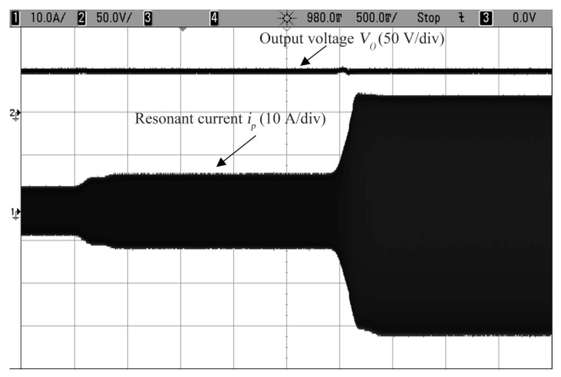
The response of the closed-loop system with M changes in the sequence of 24.1 µH–14.1 µH–7.1 µH is shown in Figure 26. The control aim is to maintain the output voltage stable at 48 V.
Figure 26 shows that the output voltage Vo is controlled at 48 V with mutual inductance variation. When the system has a relatively strong coupling (M equals 24.1 µH), the amplitude of the resonant current ip, is controlled low to limit the power transfer. However, when the system has a weak coupling (M equals 7.1 µH), the amplitude of ip was controlled high to guarantee required power transfer. It will be beneficial for reducing unnecessary power losses in the primary coil. Therefore, the control method can not only obtain good anti-perturbation performance for mutual inductance variation, but also optimize the energy transmission performance.
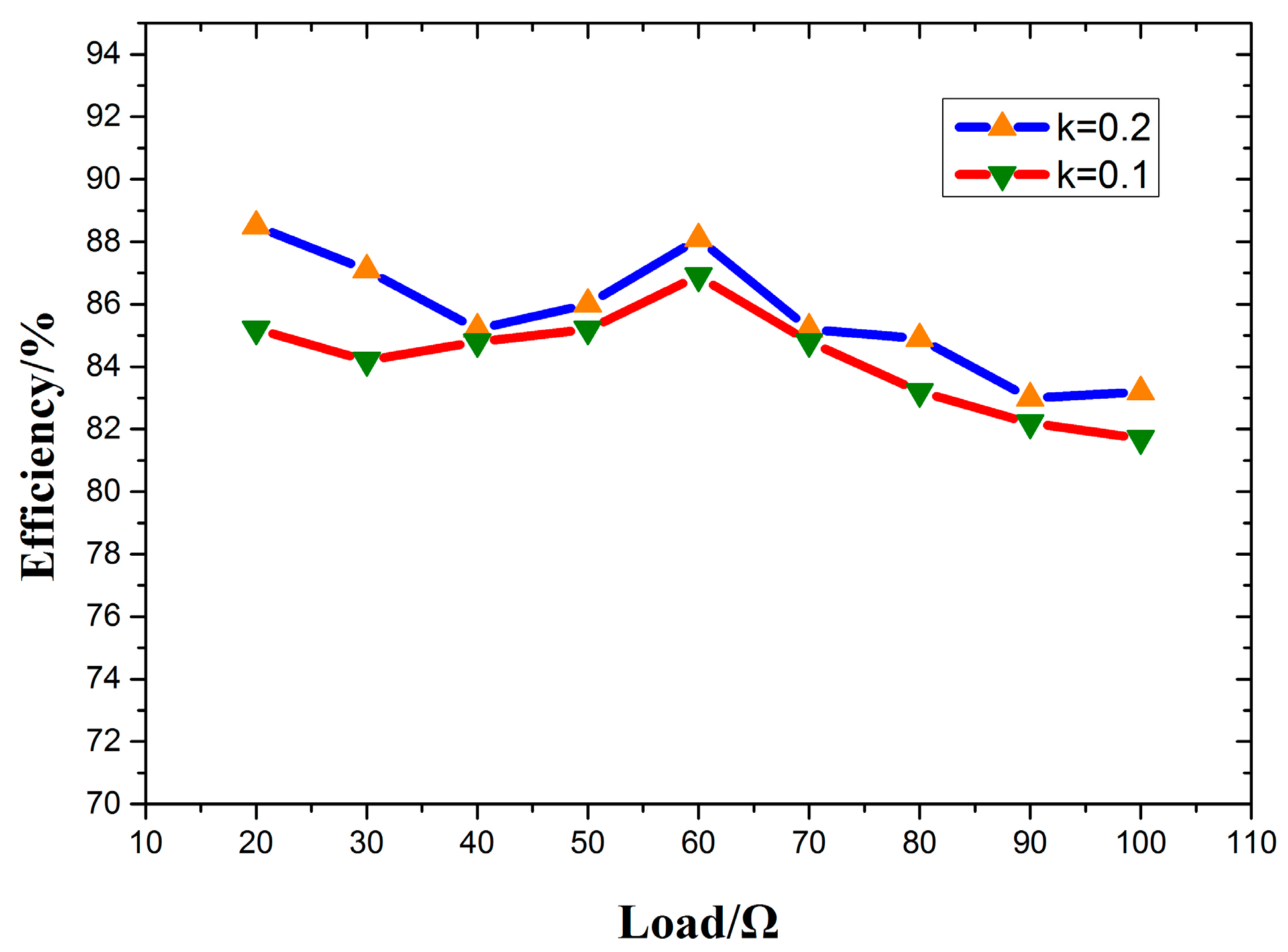
To evaluate the controller performance on system efficiency, an experimental test was carried out. In the robust control, system efficiency is measured on the condition of coupling coefficient and load variation. The experimental results can be shown in Figure 27.
As can be seen, when coupling coefficient equals 0.1, system efficiency varied from 81% to 85% with load resistance variation from 10 to 100. When coupling coefficient equals 0.2, system efficiency varied from 83% to 88%. The results show this robust control method can achieve relatively high efficiency. With the robust control, the required resonant current can be regulated according to actual load requirement. The power losses on the primary and secondary coil can be significantly reduced when compared with traditional constant resonant current mode.
9. Conclusions
Aiming at improving the robustness for moving Rrobot wireless power supplies, this paper proposes a H∞ control method for a WPT system with multiple uncertain parameters variations. The main results of this paper can be summarized as follows:
- (1)
- A special composite Upper LFT method is proposed to solve uncertain mutual inductance detachment problem. This control method can achieve good robust performance whether the parameters change abruptly or in the continuous variation condition. The response time can be reduced to less than 15 ms. It is the fastest response speed for robust control in a WPT system
- (2)
- This paper proposes a virtual buck converter for phase-shifted regulation to replace the real buck converter. This equivalent regulation method is especially useful for developing advanced controller such as robust control and adaptive control in power electronics converter.
- (3)
- This paper is mainly aimed at provide a stable and robust wireless power connection for robot charging, but this method is not limited to robots, as it can significantly improve the robustness characteristics and system efficiency on the condition that there exists frequent relative movement between the primary and secondary side.
Acknowledgments
The research work is financially supported by the research fund of National Natural Science Foundation of China (Nos. 51377187, 51377183)
Author Contributions
Author Qichang Duan contributed the main idea of this paper and provided guidance and supervision. Author Yanling Li implemented the research, performed the analysis, did the experiments and wrote the paper. Author Yang Zou provides controller evaluation and experimental date analysis.
Conflicts of Interest
The authors declare no conflict of interest.
Appendix A
Substituting the LFT blocks of uncertain parameters in Figure 5 into the system GSSA model, the GSSA model with uncertain parameters can be obtained. Then the LFT method can be utilized to detach the uncertain parameters from the nominal GSSA model. One state equation is selected as an example to illustrate the process. The state equation of iS is a relative cross-coupling equation due to including the product of multiple uncertain parameters. It can be shown as:
Due to the uncertain mutual inductance M existing in denominator of state equation, it is difficult to be extracted out. This paper uses a composite Upper LFT structure to detach the uncertain part from system state equation. The block diagram of the GSSA model is shown in Figure A1.
Define
By extracting out the uncertainty coefficients from the nominal part of the model, an individual uncertainty model of (A1) can be obtained and its state space equations are shown as below:
where:
Figure A1.
Block diagram of the state equation of iS.
Hitherto the uncertainties are extracted out. Moreover, the outputs and inputs of the perturbation block is given as:
where:
The uncertainties in the whole system can be extracted out in the same way. By extracting out these uncertain coefficients from the nominal part of the model, an overall uncertainty model can be obtained. The whole uncertainty model can be represented in the form of an upper LFT FU(Gnom, Δ).
References
- Budhia, M.; Boys, J.T.; Covic, G.A.; Huang, C.-Y. Development of a single-sided flux magnetic coupler for electric vehicle IPT charging systems. IEEE Trans. Ind. Electron. 2013, 60, 318–328. [Google Scholar] [CrossRef]
- Elliott, G.A.J.; Raabe, S.; Covic, G.A.; Boys, J.T. Multiphase pickups for large lateral tolerance contactless power-transfer systems. IEEE Trans. Ind. Electron. 2010, 57, 1590–1598. [Google Scholar] [CrossRef]
- Ke, Q.; Luo, W.; Yan, G.; Yang, K. Analytical Model and Optimized Design of Power Transmitting Coil for Inductively Coupled Endoscope Robot. IEEE Trans. Biomed. Eng. 2016, 63, 694–706. [Google Scholar] [CrossRef] [PubMed]
- Shi, Y.; Yan, G.; Chen, W.; Zhu, B. Micro-intestinal robot with wireless power transmission: Design, analysis and experiment. Comput. Biol. Med. 2015, 66, 343–351. [Google Scholar] [CrossRef] [PubMed]
- Liu, C.; Chau, K.T.; Zhang, Z.; Qiu, C.; Li, W.L.; Ching, T.W. Wireless power transfer and fault diagnosis of high-voltage power line via robotic bird. J. Appl. Phys. 2015, 117, 17D521. [Google Scholar] [CrossRef]
- Lee, S.G.; Hoang, H.; Choi, Y.H.; Bien, F. Efficiency improvement for magnetic resonance based wireless power transfer with axial-misalignment. Electron. Lett. 2012, 48, 339–340. [Google Scholar] [CrossRef]
- Villa, J.L.; Sallan, J.; Osorio, J.F.S.; Llombart, A. High-Misalignment Tolerant Compensation Topology for ICPT Systems. IEEE Trans. Ind. Electron. 2012, 59, 945–951. [Google Scholar] [CrossRef]
- Raabe, S.; Covic, G.A. Practical Design Considerations for Contactless Power Transfer Quadrature Pick-Ups. IEEE Trans. Ind. Electron. 2013, 60, 400–409. [Google Scholar] [CrossRef]
- Kissin, M.L.G.; Huang, C.Y.; Covic, G.A.; Boys, J.T. Detection of the Tuned Point of a Fixed-Frequency LCL, Resonant Power Supply. IEEE Trans. Power Electron. 2009, 24, 1140–1143. [Google Scholar] [CrossRef]
- Li, Y.L.; Sun, Y.; Dai, X. μ-Synthesis for Frequency Uncertainty of the ICPT System. IEEE Trans. Ind. Electron. 2013, 60, 291–300. [Google Scholar] [CrossRef]
- Pijl, F.V.D.; Bauer, P.; Castilla, M. Control Method for Wireless Inductive Energy Transfer Systems with Relatively Large Air Gap. IEEE Trans. Ind. Electron. 2013, 60, 382–390. [Google Scholar] [CrossRef]
- Madawala, U.K.; Thrimawithana, D.J. A Bidirectional Inductive Power Interface for Electric Vehicles in V2G Systems. IEEE Trans. Ind. Electron. 2011, 58, 4789–4796. [Google Scholar] [CrossRef]
- Moradewicz, A.J.; Kazmierkowski, M.P. Contactless Energy Transfer System with FPGA-Controlled Resonant Converter. IEEE Trans. Ind. Electron. 2010, 57, 3181–3190. [Google Scholar] [CrossRef]
- Van Der Pijl, F.F.; Castilla, M.; Bauer, P. Adaptive Sliding-Mode Control for a Multiple-User Inductive Power Transfer System without Need for Communication. IEEE Trans. Ind. Electron. 2013, 60, 271–279. [Google Scholar] [CrossRef]
- Hsu, J.U.W.; Hu, A.P.; Swain, A. Fuzzy logic-based directional full-range tuning control of wireless power pickups. IET Power Electron. 2012, 5, 773–781. [Google Scholar] [CrossRef]
- Neath, M.J.; Swain, A.K.; Madawala, U.K.; Thrimawithana, D.J. An Optimal PID Controller for a Bidirectional Inductive Power Transfer System Using Multiobjective Genetic Algorithm. IEEE Trans. Power Electron. 2014, 29, 1523–1531. [Google Scholar] [CrossRef]
- Huang, C.Y.; Boys, J.T.; Covic, G.A. LCL Pickup Circulating Current Controller for Inductive Power Transfer Systems. IEEE Trans. Power Electron. 2013, 28, 2081–2093. [Google Scholar] [CrossRef]
- Wang, C.S.; Covic, G.A.; Stielau, O.H. Investigating an LCL load resonant inverter for inductive power transfer applications. IEEE Trans. Power Electron. 2004, 19, 995–1002. [Google Scholar] [CrossRef]
- Hu, A.P. Modeling a contactless power supply using GSSA method. In Proceedings of the IEEE International Conference on Industrial Technology, Victoria, Australia, 10–13 February 2009; IEEE: Piscataway, NJ, USA, 2009; pp. 1–6. [Google Scholar]
- Ortega, M.G.; Rubio, F.R. Systematic design of weighting matrices for the H∞, mixed sensitivity problem. J. Process Control 2004, 14, 89–98. [Google Scholar] [CrossRef]
Figure 1.
LCL type WPT system.

Figure 2.
Phase-shifted regulation mode.
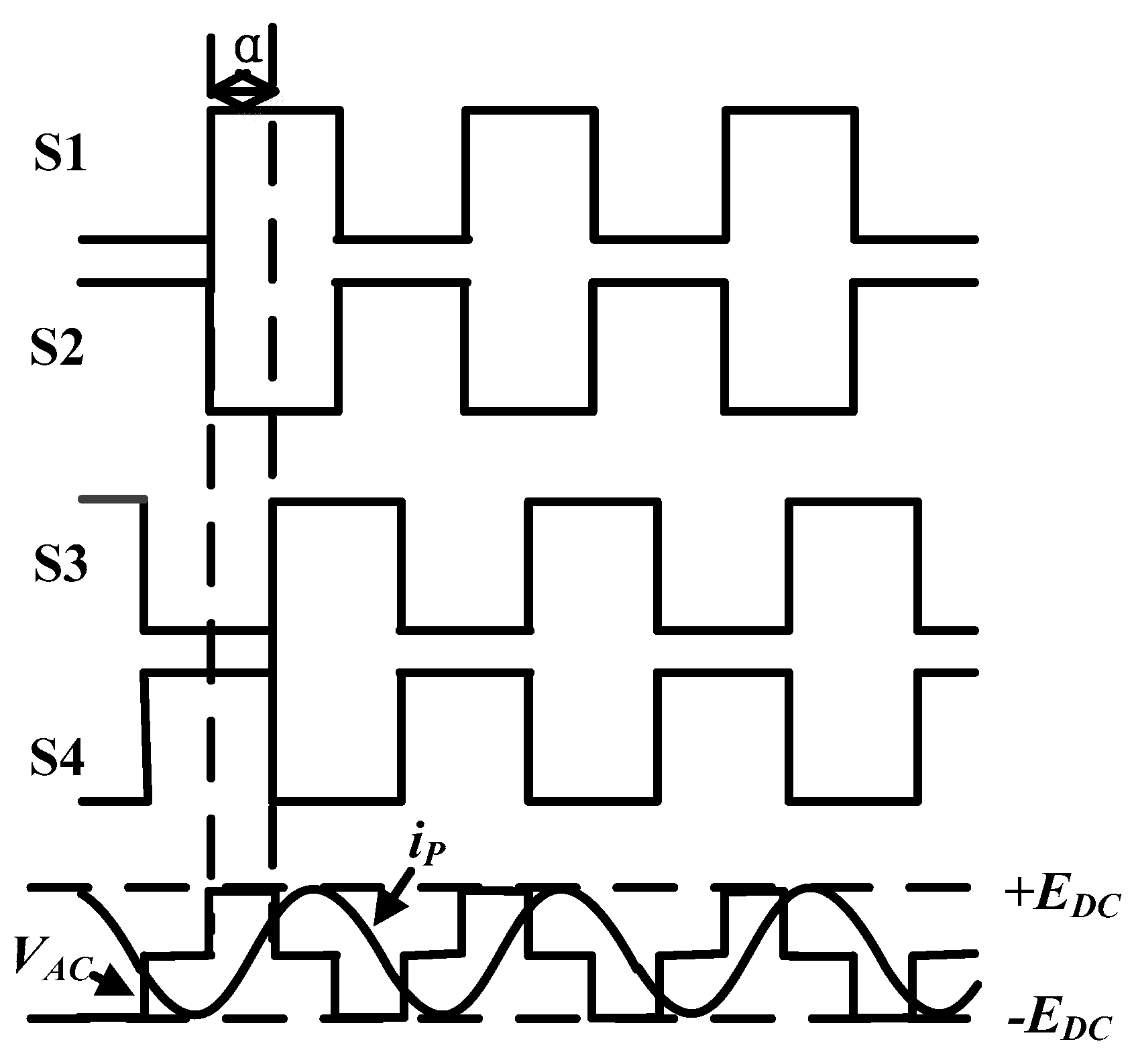
Figure 3.
Virtual buck converter scheme for the robust control.

Figure 4.
Equivalent circuit of the LCL type WPT system.
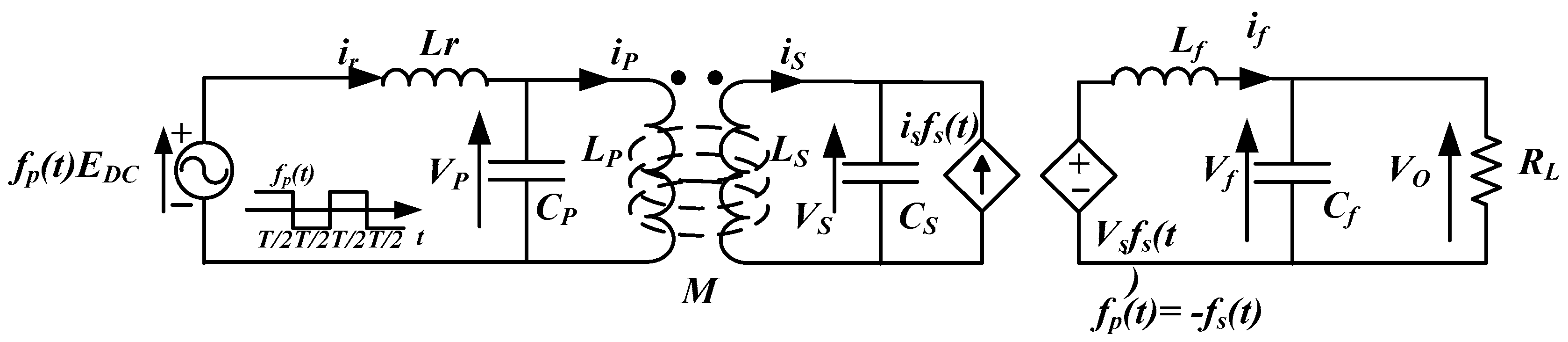
Figure 5.
Upper LFT blocks of the uncertain parameters.
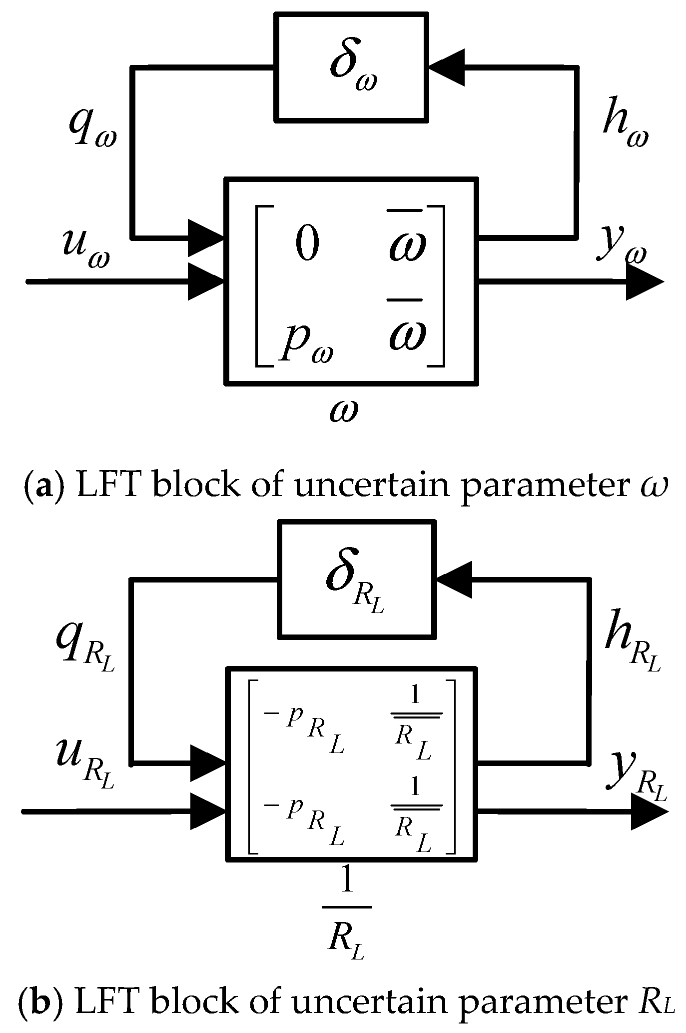
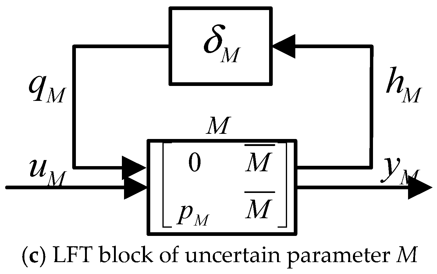
Figure 6.
System model after uncertain part detachment.
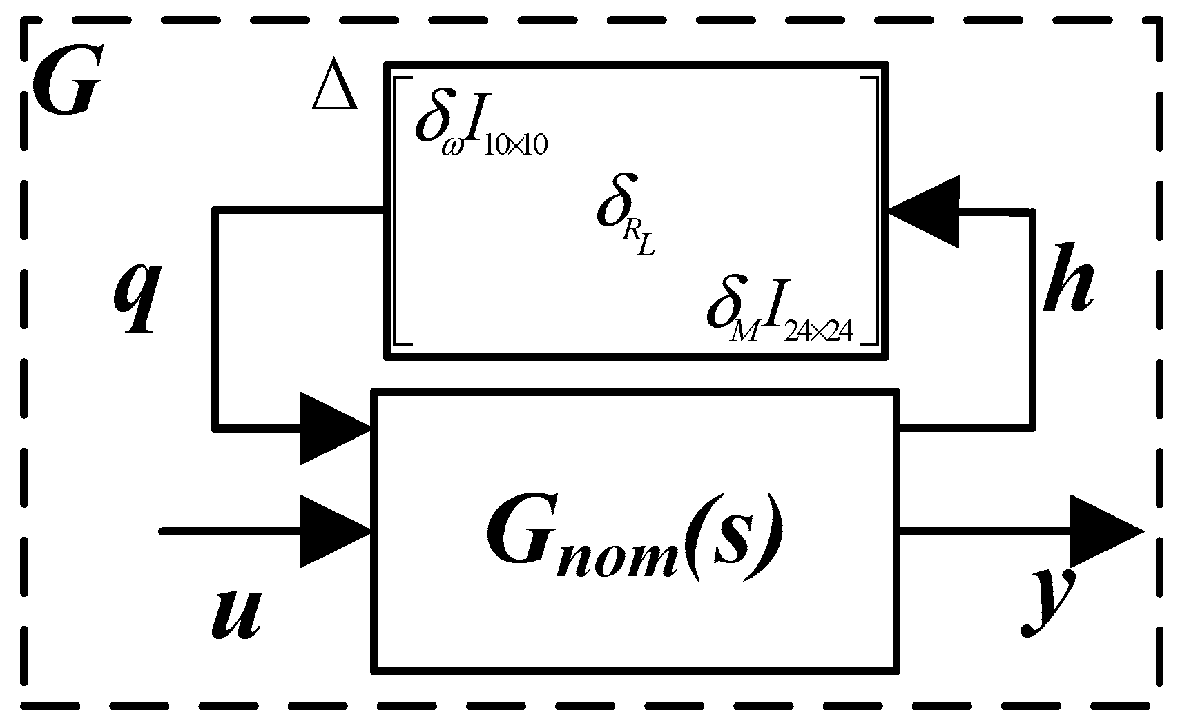
Figure 7.
Generalized plant of the mixed sensitivity (S/R) design.

Figure 8.
H∞ controller configuration.

Figure 9.
Design procedure of a H∞ suboptimal controller.
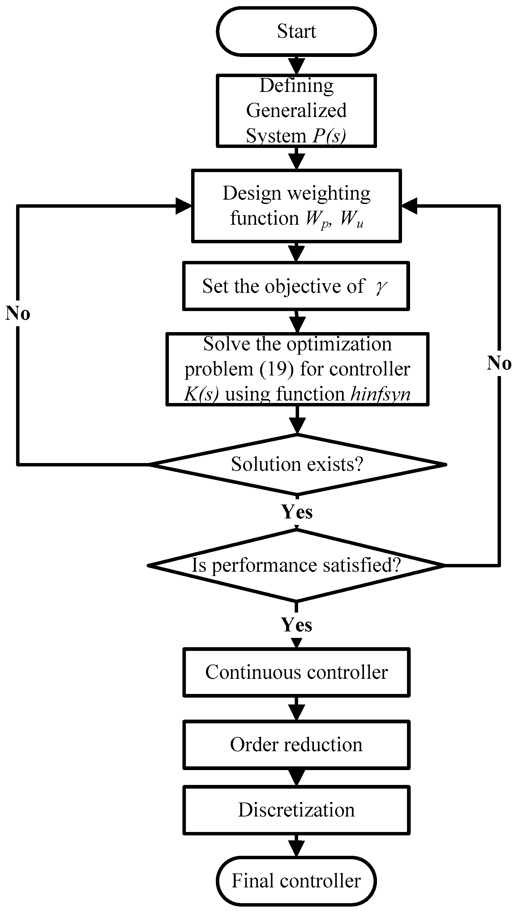
Figure 10.
The standard H∞ configuration.
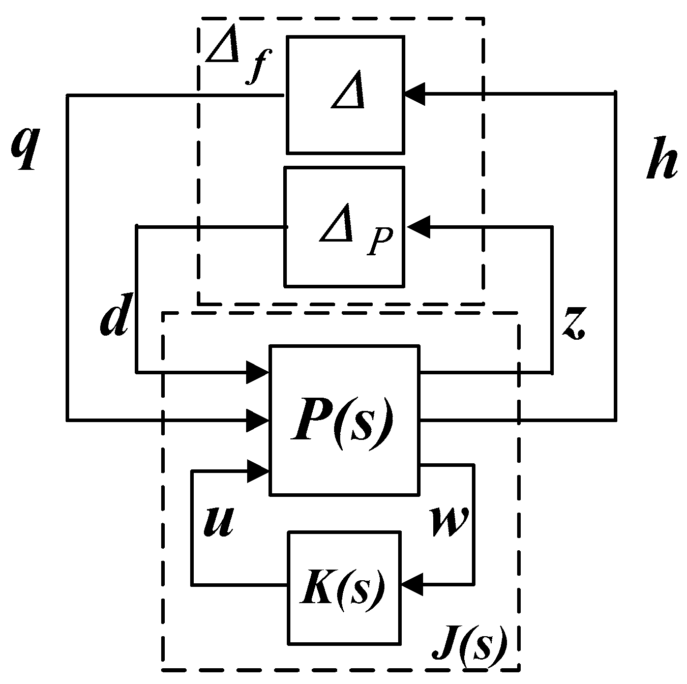
Figure 11.
Robust stability analysis with upper and lower bound of µ.
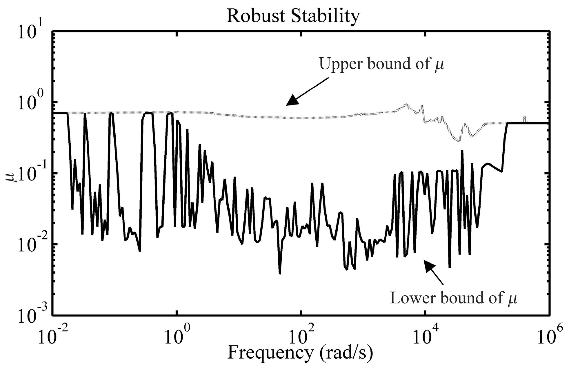
Figure 12.
Robust performance analysis with upper and lower bound of µ.
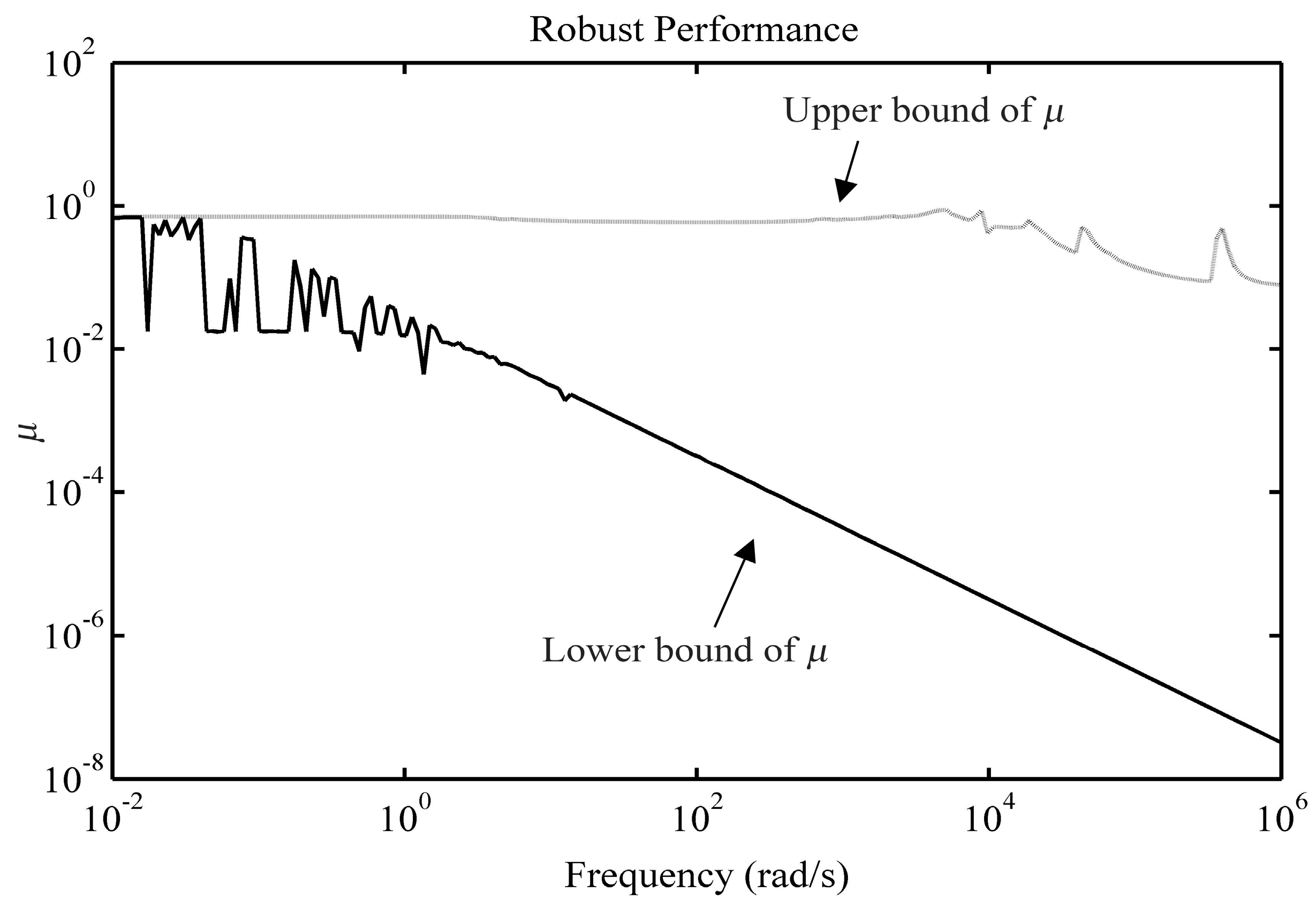
Figure 13.
Simulation model of WPT system.
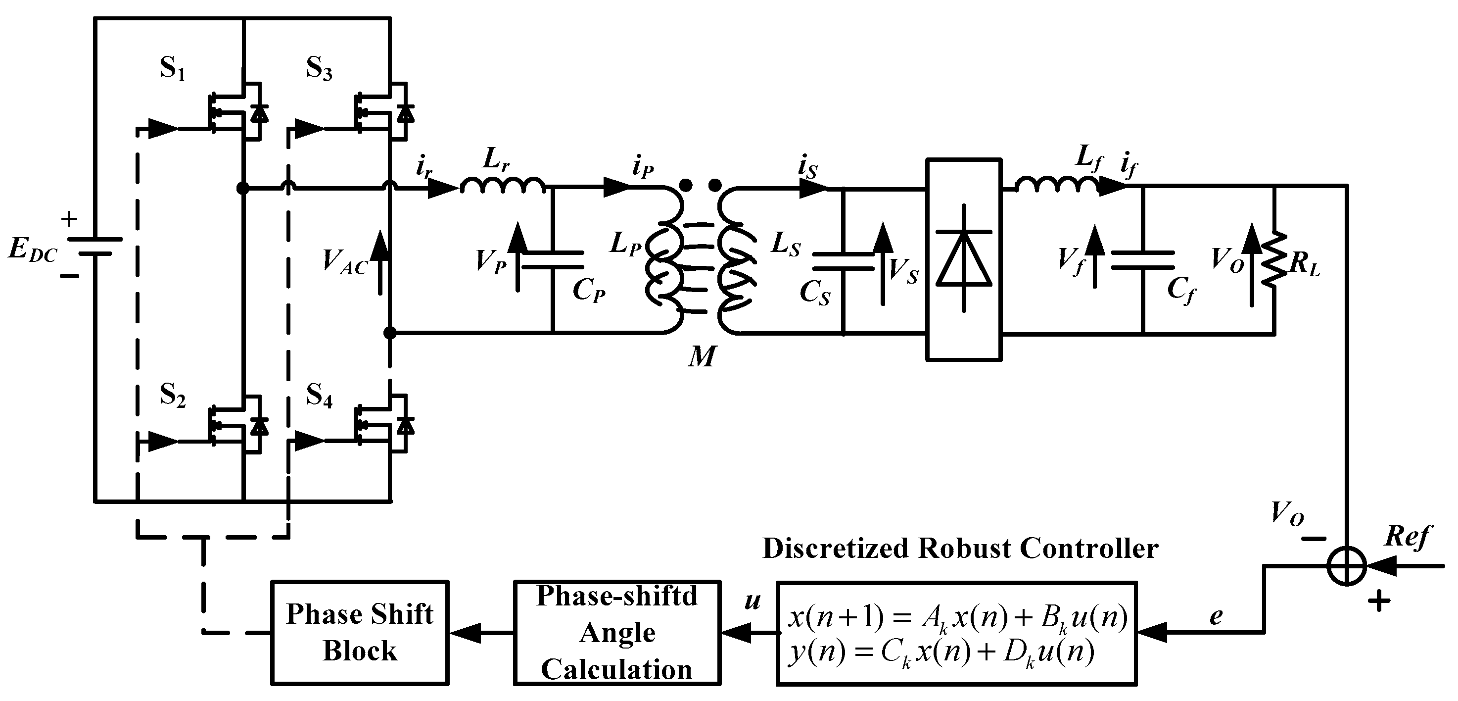
Figure 14.
Simulation response of the H∞ control system with ramp reference.

Figure 15.
Simulation response of the H∞ control system with reference variation.

Figure 16.
Simulation response of the H∞ control system with load variations.
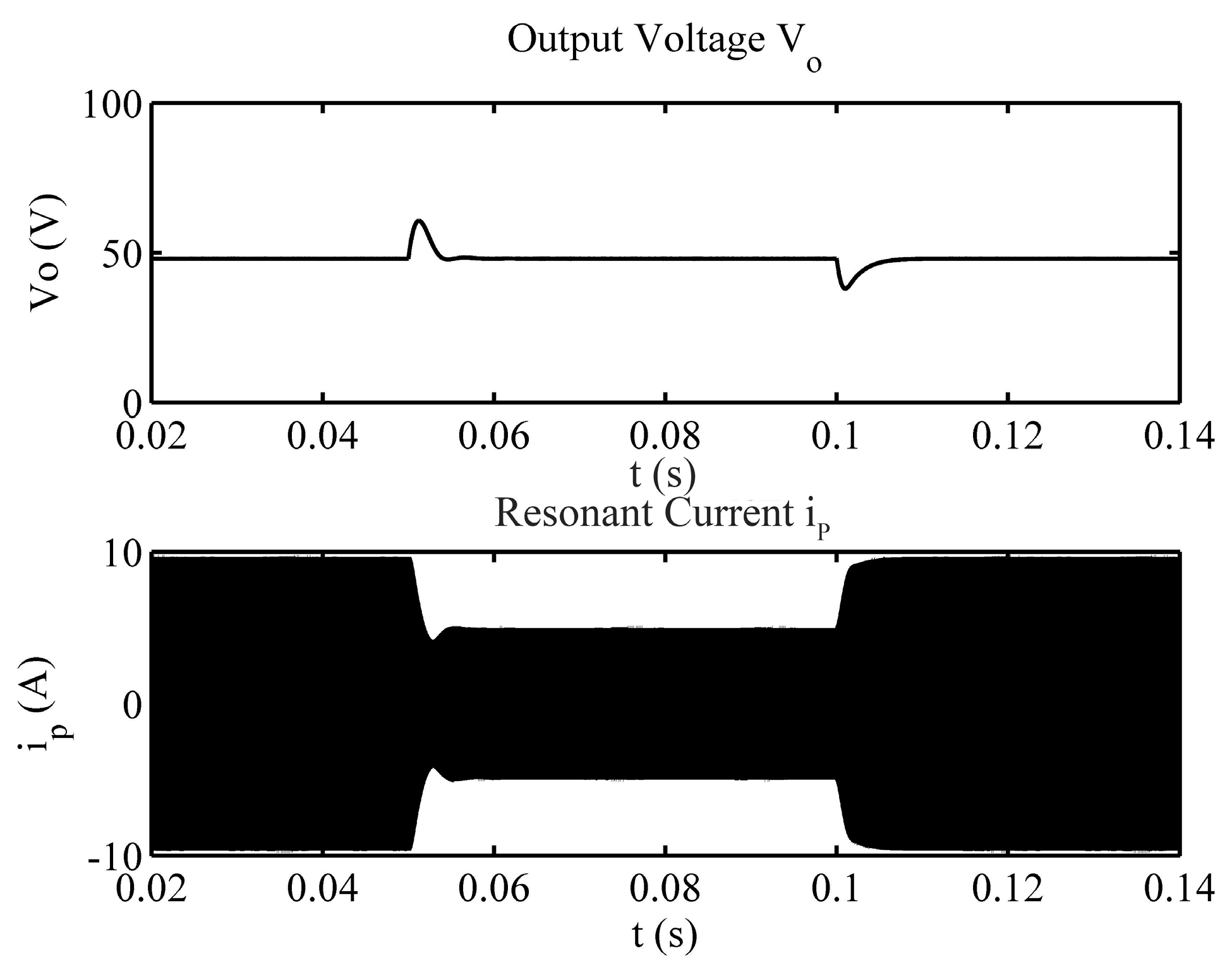
Figure 17.
Steady state waveforms with 50 Ω load.
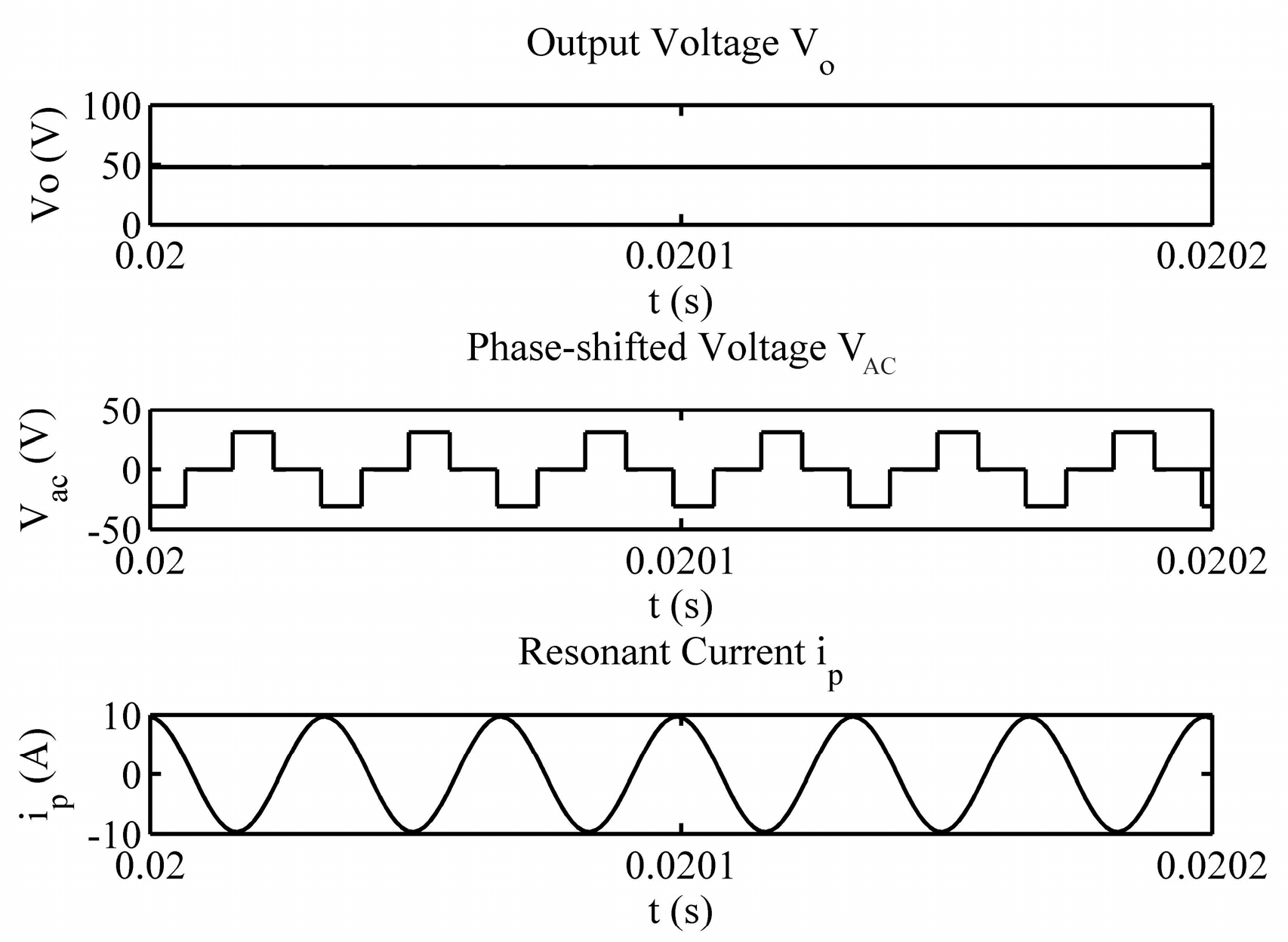
Figure 18.
Steady state waveforms with 100 Ω load.

Figure 19.
Experimental system configuration and photo.
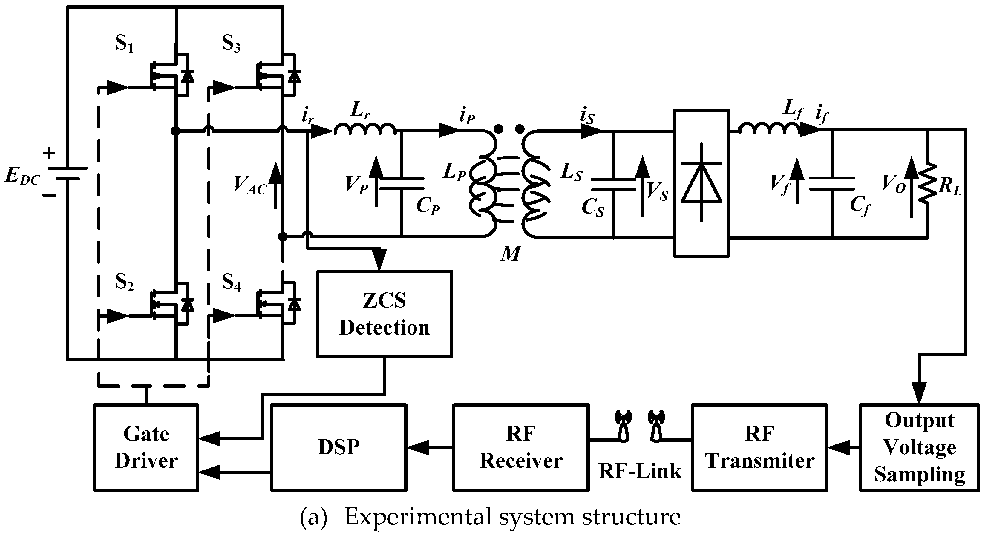

Figure 20.
Experimental response of the H∞ control system with ramp reference.
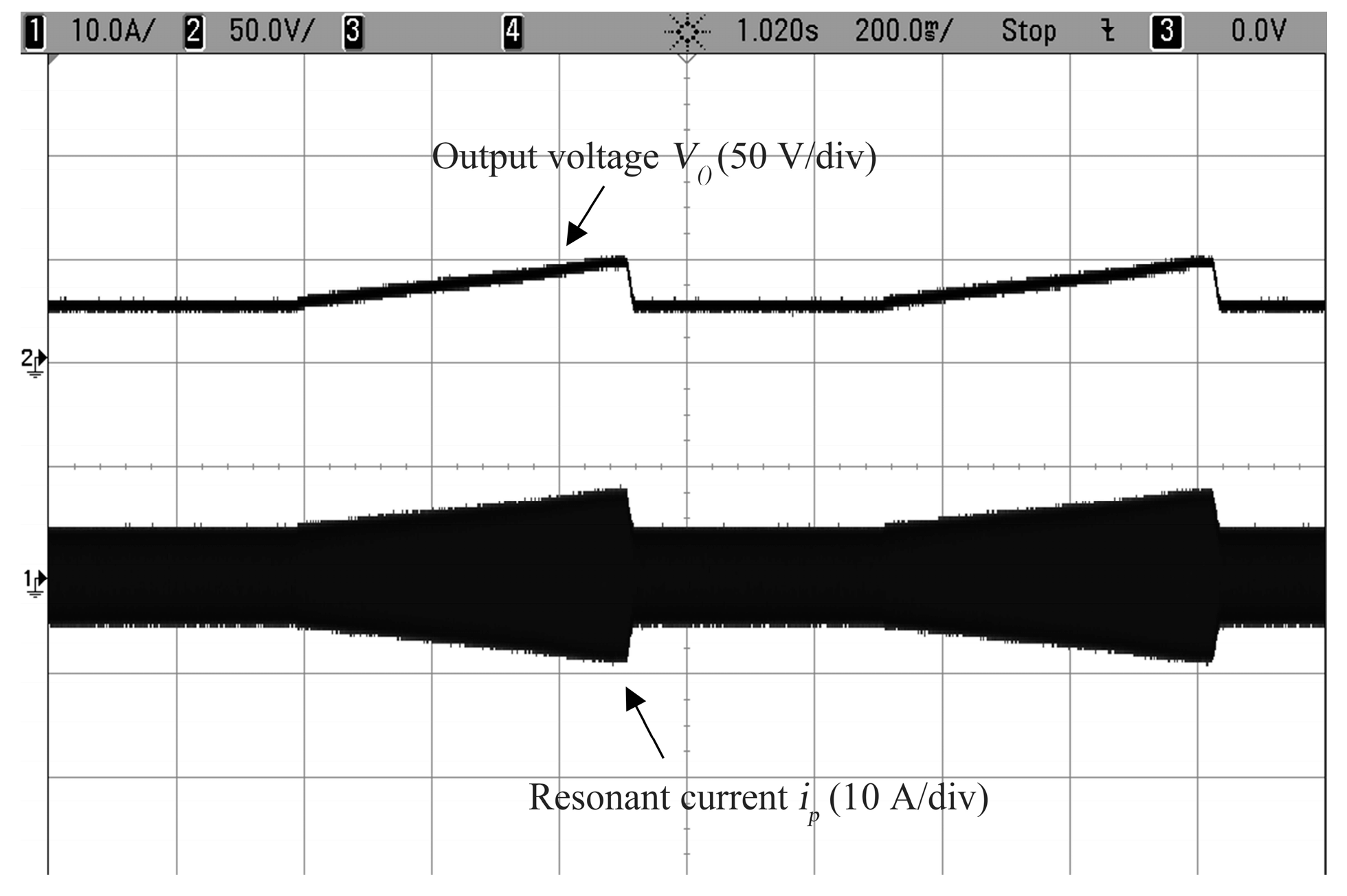
Figure 21.
Experimental response of the H∞ control system with reference variation.

Figure 22.
Experimental response of the H∞ control system with load variations.
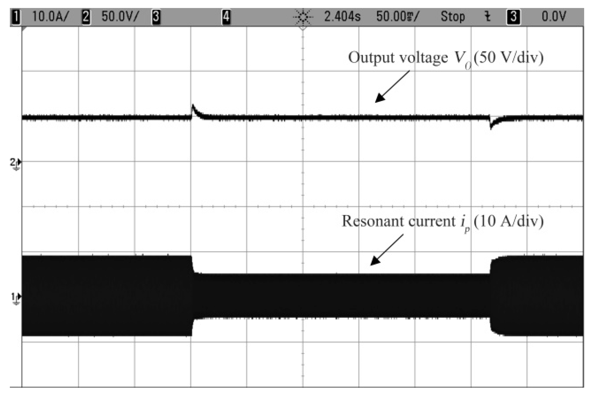
Figure 23.
Steady state waveforms under load of 50 Ω.
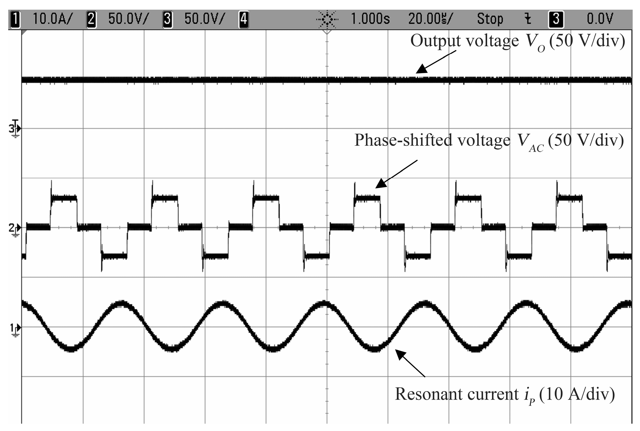
Figure 24.
Steady state waveforms under load of 100 Ω.
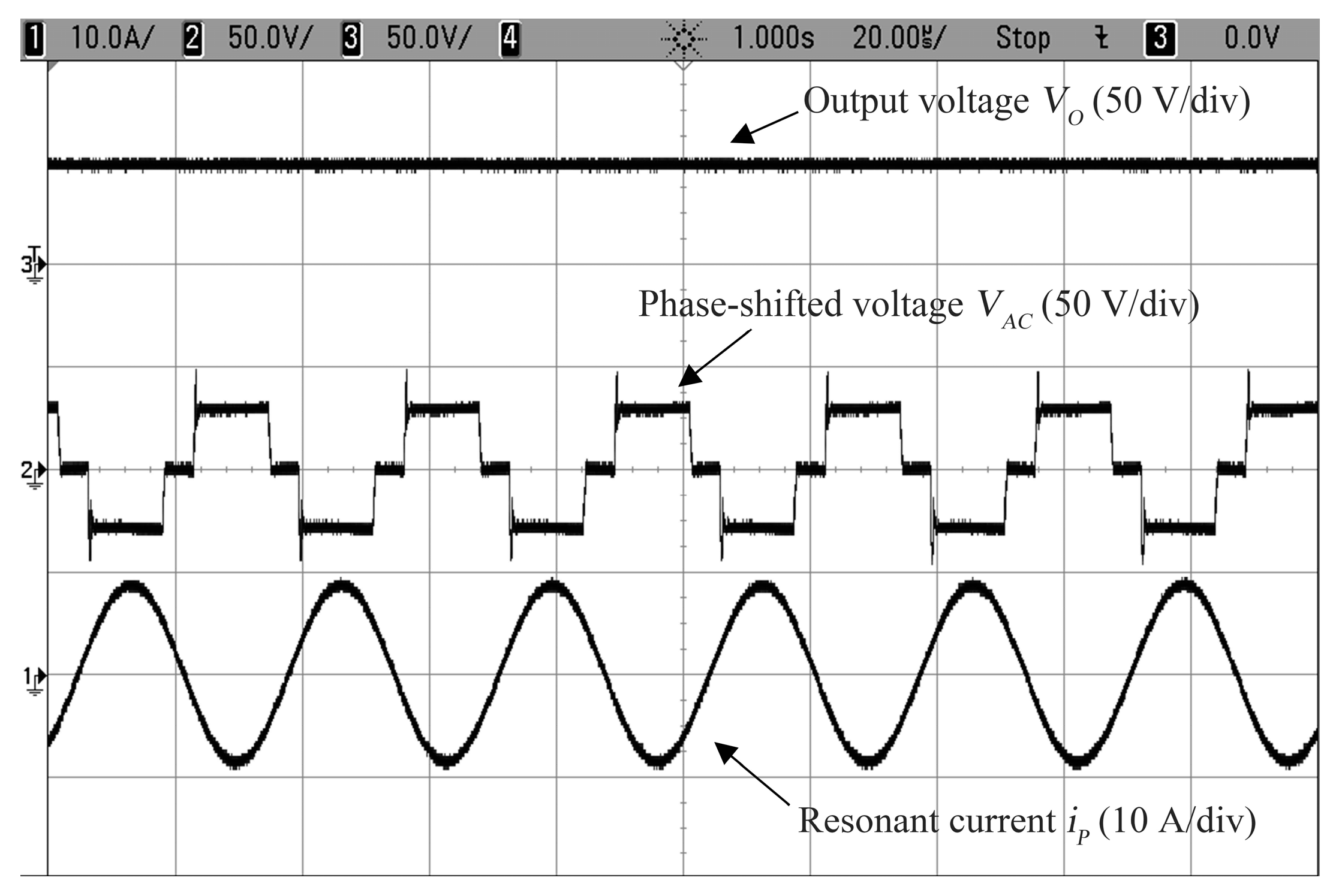
Figure 25.
Mutual inductance variation test.

Figure 26.
Experimental response of the H∞ control system with mutual inductance variation.

Figure 27.
System efficiency variation with load and coupling coefficient variation.

Table 1.
The uncertain system parameters.
| Parameter | Nominal Value | Uncertain Interval | Unit |
|---|---|---|---|
| ω | 190,380 | [188,495, 191,637] | rad/s |
| RL | 50 | [25, 75] | Ω |
| M | 14.1 | [7, 25] | µH |
Table 2.
Circuits parameters.
| Parameters | Value | Unit |
|---|---|---|
| Lr | 220 | µH |
| LP | 110 | µH |
| LS | 110 | µH |
| Lf | 1000 | µH |
| RLr | 0.115 | Ω |
| RLp | 0.115 | Ω |
| RLs | 0.115 | Ω |
| CP | 0.374 | µF |
| CS | 0.25 | µF |
| Cf | 22 | µF |
| EDC | 31.5 | V |
© 2017 by the authors. Licensee MDPI, Basel, Switzerland. This article is an open access article distributed under the terms and conditions of the Creative Commons Attribution (CC BY) license (http://creativecommons.org/licenses/by/4.0/).
Share and Cite
MDPI and ACS Style
Li, Y.; Duan, Q.; Zou, Y. High Robustness Control for Robotic Wireless Power Transfer Systems with Multiple Uncertain Parameters Using a Virtual Buck Converter. Energies 2017, 10, 517. https://doi.org/10.3390/en10040517
AMA Style
Li Y, Duan Q, Zou Y. High Robustness Control for Robotic Wireless Power Transfer Systems with Multiple Uncertain Parameters Using a Virtual Buck Converter. Energies. 2017; 10(4):517. https://doi.org/10.3390/en10040517
Chicago/Turabian StyleLi, Yanling, Qichang Duan, and Yang Zou. 2017. "High Robustness Control for Robotic Wireless Power Transfer Systems with Multiple Uncertain Parameters Using a Virtual Buck Converter" Energies 10, no. 4: 517. https://doi.org/10.3390/en10040517
Note that from the first issue of 2016, this journal uses article numbers instead of page numbers. See further details here.