
Research on Stochastic Optimal Operation Strategy of Active Distribution Network Considering Intermittent Energy


1
Key Laboratory of Control of Power Transmission and Conversion, Ministry of Education, Department of Electrical Engineering, Shanghai Jiao Tong University, Shanghai 200240, China
2
State Grid Jiangxi Nanchang Power Supply Company, Nanchang 330000, China
*
Author to whom correspondence should be addressed.
Energies 2017, 10(4), 522; https://doi.org/10.3390/en10040522
Submission received: 30 January 2017
/
Revised: 28 March 2017
/
Accepted: 30 March 2017
/
Published: 12 April 2017
(This article belongs to the Special Issue Electric Power Systems Research 2017)
Abstract
:Active distribution networks characterized by high flexibility and controllability are an important development mode of future smart grids to be interconnected with large scale distributed generation sources including intermittent energies. However, the uncertainty of intermittent energy and the diversity of controllable devices make the optimal operation of distribution network a challenging issue. In this paper, we propose a stochastic optimal operation strategy for distribution networks with the objective function considering the operation state of the distribution network. Both distributed generations and flexible loads are taken into consideration in our strategy. The uncertainty of the intermittent energy is considered in this paper to obtain an optimized operation and an efficient utilization of intermittent energy under the worst scenario. Then, Benders decomposition is used in this paper to solve the two-stage max-min problem for stochastic optimal operation. Finally, we test the effectiveness of our strategy under different scenarios of the demonstration project of active distribution network located in Guizhou, China.
1. Introduction
In recent years, the access of intermittent energy, such as wind and solar, keeps increasing in distribution networks. Under such a circumstance, active distribution networks (ADNs) characterized by high distributed generation penetration and high control requirements have been widely accepted as an important development mode of future smart grids [1,2]. Compared with traditional distribution networks, active distribution networks have more controllable equipment, including energy storage systems, flexible loads, and other distributed generation sources. In order to ensure the optimal operation of active distribution networks, reasonable arrangement for the output of different types of controllable equipment is essential [3]. However, in active distribution network, the uncertainty of intermittent energy makes the traditional deterministic power system to a random-deterministic coupling power system. At the same time, distribution network operation concerns more about the economic benefit and the operating state, which brings great challenge to the power system optimization.
To realize optimal operation of an ADN considering the uncertainty of intermittent energy, two key issues need to be taken into consideration: the uncertainty of intermittent energy and the coordination between the risk and the economic benefit of the ADN.
Intermittent energy power forecasting is usually introduced to optimal operation to achieve a more precisely control. There are a variety of models and prediction methods such as artificial neural networks (ANN), Kalman filtering method and fuzzy logic method used in power forecasting to obtain accurate predictions [4]. However, the forecasting for intermittent energy influenced by complex factors related to the environment is still a challenging problem. Researchers have done a lot of works on optimal operation considering the uncertainty of intermittent energy including stochastic unit commitment (SUC) [5,6,7] or stabilizing the unpredicted power fluctuation by energy storage system and demand response [8]. Such as both [6,7], the uncertainty of wind power or load is divided into several scenarios which represent different wind power output probability. It is obvious that the accuracy of the solution mainly depends on the selection of uncertainty scenarios.
To deal with the coordination between the risk and the economic benefits in power system, most researchers focus on minimizing the operating cost [9,10]. Like [9], it takes the minimization of total UC schedule cost as main consideration, while considering the alleviation of wind power curtailment and the risk of inclusion of wind energy generation at the same time. Due to the different requirements of the system operators, some other objectives are also used such as minimizing the variance for the risk-averse case or even multi-objectives [11,12,13]. Unlike the transmission network concerns more about the operating cost, one of the priorities of ADN is to improve the economic benefits brought by different controllable devices. At the same time, the operational characteristics of ADN like the peak-valley difference and the network loss are also concerned. The reduction of peak-valley difference and network loss can reduce the reserve capacity of the transmission network and improve the efficiency of energy usage, which will also improve the economic efficiency of ADN. So, the objective function presented in this paper will take the peak-valley difference, the network loss and the economic benefits brought by different controllable devices into consideration. In order to avoid the risk of optimization due to intermittent energy prediction errors, the uncertainties of intermittent energies are also taken into account to ensure optimal operation of ADN under the worst scenario.
Due to the complexity of both controllable equipment and objective function, the optimal operation problem formulated as a mixed-integer linear programming (MILP) is non-deterministic polynomial-time hard (NP-hard). Several algorithms such as the hybrid genetic algorithm [14], differential evolution algorithm [15], discrete particle swarm optimization [11,16] and artificial bee colony [17] are used to solve the problem. However, the intelligent algorithms mentioned above have a common problem. They may not be able to obtain the optimal solution but a better one instead which will lead to a considerable uncertainty of the optimal result. Outer approximation methods are used in [18,19] to solve the mixed-integer nonlinear programming (MINLP) problem of unit commitment. Some researchers also have applied other methods such as Lagrangian relaxation (LR) and Benders decomposition (BD) to solve the problem [20,21]. This type of algorithm requires certain characteristics for constraints or objective functions, such as convex functions, etc. So it cannot be applied to solve all problems. But it is an effective way to simplify the problem-solving process.
In this paper, we mainly aimed to integrate the controllable resources in ADN to achieve a more efficient power system operation. As discussed before, the objective function for optimization will take the economic benefits of DGs, two key characteristics of ADN and the uncertainty of intermittent energies into consideration. While taking the constraint of power flow and so on into consideration, the optimization problem will form a complicated non-linear problem. To simplify the nonlinear programming problem proposed, we reformulated the objective function into a two-stage max-min problem. Benders decomposition is introduced to the approach to simplify the complexity of sub-problem. The algorithm can limit the uncertainty of intermittent energy output according to the requirement and find out the optimal controllable resource output.
The remaining part of this paper is organized as follows: Section 2 provides mathematical modeling of an optimal operation strategy. Section 3 introduces the solution approach based on Benders decomposition. The case study and optimization results are discussed in Section 4, combined with the active distribution network demonstration project located in Guizhou, China. Section 5 concludes with the main results of this paper.
2. Mathematical Formulation
In this section, we establish the optimization formulation for optimal operation of active distribution network considering multi-controllable resources. Combined with the conditions of Guizhou demonstration project, direct load control for flexible loads are also taken into account in this formulation as an adjustable resource for distribution network. In order to simplify the complexity of flexible load modeling, we will divide flexible load including Heating, Ventilation and Air Conditioning (HVAC) devices and electric vehicles into two categories, in accordance with their characteristics and unified it with the distributed generation model. This can simplify the optimization formulation.
In general, there are three kinds of distributed generations in a distribution network: power regulation generations, energy storage systems, and intermittent energy. Different types of distributed generations correspond to different constraints. In active distribution network, intermittent energy is generally desirable to achieve the maximum power consumption, so in this paper we only consider the uncertainty of intermittent energy. It won’t be taken as one of the controllable resources.
For power regulation generations such as thermal power generations and hydropower generations, the constrains mainly include the ramp-up rate, ramp-down rate, maximum power limit and minimum power limit in the form of (1)–(3):
In this paper, we lump flexible loads such as HVAC together with former power regulation generations as ‘power regulation devices’. For flexible load such as HVAC, the instantaneous power will keep changing when it turns on or off to maintain the room temperature. However, we only concern about the average power when taking optimization instead of instantaneous power. The average power for a HVAC when the set-temperature is can be expressed as (4) [22]:
is the equivalent thermal resistance for (degrees Celsius/W). is the ambient temperature. is the set temperature for . is the conversion efficiency from electricity to heat. We assume that the set temperature for a customer can be adjusted from to when taking customers’ comfort into consideration. The adjustable power range can be expressed as (5) and (6):
So constraint for flexible load such as HVAC can be expressed as (7):
Considering that the set temperature of HVAC can be changed instantaneously, Constraints (1) and (2) can be neglected or set . is a large number. Other flexible loads like brightness adjustable lighting can also be expressed as (7).
Apart from former ‘power regulation devices’, energy storage systems (ESSs) are another kind of distributed energy in ADNs. This type of equipment can realize the energy transfer between different time spans by charging and discharging. The characteristics of such equipment can be described by the index of state of charge (SOC). The constraints for SOC can be expressed as (8)–(10):
Here we introduce into the formulation to make sure all variables are non-negative and . It should be noticed that, is usually used to express the SOC for energy storage device by the end of time period . But to simplify the future solution process, while not affecting the variables, in this paper is defined as the SOC before the start of time period .
In this paper, we merge flexible load with energy storage characteristics such as water heater and electric vehicle with energy storage system as ‘energy storage devices’. For flexible load such as water heater, it is usually used once a day. And it is necessary to reach a specified temperature at a specified time. The state of household water heater can be expressed by temperature . The state of the water heater can be expressed as (11):
is the desired temperature for water heater . is the initial temperature for water heater . If we take the sensitivity of temperature to energy into account, the constraints for water heater can also be expressed as (8)–(10). As the water heater cannot release energy, constraint (9) need to be replaced by (12):
SOC limit for a water heater is when and , when . The rated capacity can be expressed as:
is the energy required for the temperature of the water heater increased by one degree. Other flexible load like electric vehicle is similar to energy storage battery. So it is much easier to be reformulated as the mode of ESS. To reflect the customers’ requirement, an extra constraint will be added to origin constraints. The SOC of an electric vehicle needs to arrive a specific value at specific time as expressed in (14).
The formula can also be meaningful for a BESS. We can assume that BESS should return to the initial state after a cycle of operation to support a continuous operation for next time span. The model of energy storage devices when electric vehicles are merged can add an extra constraint shown as (15).
Apart from former model merging, the uncertainty for the intermittent energy is also considered in this paper described as a solution space for specify scenario. The prediction for intermittent energy is . We use the normal distribution or Cauchy distribution to describe the prediction error for intermittent energy centered on the predicted value . In this paper, we set a power deviation to make sure the probability for intermittent energy output within the deviation range to be at least 0.95. We can assume the upper deviation of the confidence interval for intermittent energy is and the lower one is . The output range for intermittent energy is . To limit the conservatism degree for intermittent power output, we introduce the method described in [23] to employ an integer as the ‘cardinality budget’. The budget is used to restrict the number of time intervals when the output of intermittent energy reaches the limitation. If equals 12, there will be less than 12 time intervals when the output reaches the limitation and for other time intervals the output will be restricted to . When , the optimization solution will be feasible with a probability greater than 0.95 [23]. In this paper, we assume and are two binary variables represent the status of deviation for . If , the output of intermittent energy will be . If , the output of intermittent energy will be , so the uncertainty set to describe the intermittent energy output can be shown as (16):
Based on the aforementioned unified model and uncertainty set of intermittent energy, the optimization formulation for optimal operation of active distribution network can be described as follow:
The former objection for optimal operation is consist by two parts. The first part includes the profit for power regulation devices (e.g., Equation (18)) and the profit for the reduction of network loss (e.g., Equation (19)). The second part includes the profit for energy storage devices (e.g., Equation (20)) and the profit for the reduction of peak-valley difference (e.g., Equation (21)).The objection is expressed by two parts because the energy storage devices mainly focuses on the effect of peak load shifting in this paper. The power regulation devices preferentially meet the network loss reduction requirement. Since the capacity of intermittent energy is relatively small in the demonstration project, the influence of its uncertainty on network loss is far less than that on peak-valley difference, so the uncertainty of intermittent energy is considered in the second part. The network loss and the peak-valley difference are two main indicators concerned by DSOs when assessing the operation of distribution network. The calculation for both indicators are described in (22)–(24):
The initial state before optimization is recorded when the output for power regulation devices maintain at current power (for flexible loads such as HVAC, maintain at the user set value), the output for energy storage devices maintain at 0 (for flexible loads such as EV, the charging time will start immediately until target is reached), the outputs for intermittent energy maintain at . Correspondingly, the optimized state is recorded when the output for power regulation devices and energy storage devices are optimized, the output for intermittent energy is when taking uncertainty into account. This is to make sure we can get an optimized result when the intermittent energy output reaches the worst scenario. is the calculation formula for network loss, which won’t be discussed in detail in this paper. to are weights for each objective. We can adjust the weights to obtain a desired target combination. Then constraint for former objection is described as a set . Some constraints are aforementioned. We will rewrite it here for a more clearly expression.
Set described in (25) is the constraint for power flow, including power flow equality constraint (e.g., Equation (36)), voltage constraint for buses (e.g., Equation (37)), transmission capacity constraints (e.g., Equation (38)). All the three constraints are used to finalize the optimization results by more stringent constraints when and . The constraints for power regulation devices are described in (26)–(28). The constraints for energy storage devices are described in (29)–(33). The complete representation for optimization formulation can be summarized as (39):
3. Solution Methodology
The formerly proposed equation it is a relatively complicated problem with several extremum calculations, thus the equation cannot be solved directly. The uncertainty for intermittent energy has increased the solving difficulty of the problem significantly. To decrease the solving complexity, Benders decomposition is introduced to this paper.
Benders decomposition is an effective method to solve complex programming problem [24]. An example of Benders decomposition can be expressed as (40):
The Benders decomposition method will decompose the original optimization problem into several parts to be solved. By the process of iteration, the solution of reformulated problem will gradually approximate the optimal solution of the original problem. This method requires the separation of variables shown as and , both variables can be vectors. and are the functions for variable . is the coefficient matrix; , is the coefficient vector. is the feasible set for variable . Then the original problem (40) can be divided into two parts by Benders decomposition. Main problem is defined on the set , it can be linear, non-linear or discrete. The problem is formulated when , where is the solution of the sub-problem:
The sub-problem should be a linear programming, shown as (42):
Firstly, the algorithm will solve the duration problem of sub-problem (42) based on a “possible solution” of the main problem (41). This “possible solution” is one of the feasible solutions for main problem. Then, additional constraints (feasibility cuts and optimal cuts) will be formed by solving the sub-problem and new constraints will be added to main problem. The formation of both cuts will be discussed in detail later. Furthermore, solve the main problem and bring the optimized results back to sub-problem (42) again, and so on. Solve the two questions alternately until the optimal solution is obtained.
Based on the aforementioned algorithm, the main problem and the sub-problem for the optimization problem proposed in this paper are expressed as (43) and (44).
Main problem:
Sub-problem:
The main problem takes the outputs of ‘power regulation devices’ as variables and the sub-problem takes the outputs of both energy storage devices and intermittent energies as variables.
Firstly, the sub-problem needs to be simplified to a single extremum value problem. In the sub-system is determined by the predicted value, therefore belongs to a constant. To express by inequality, we introduce extra variable and constraints in (45)–(47):
Therefore problem (44) can be described as (48):
Furthermore, (48) can be transformed as (49):
To solve the further min-max problem, we use the dual approach to translate the maximize problem of to a minimize problem. The solution space is defined as :
In the former equation, and correspond to the dualizing of constrains (46) and (47). and correspond to constraint (31). corresponds to constraint (30). , , correspond to constraints (29) and (32) and (33). Constraints (51) to (56) correspond to initial variables , , and . In the dual problem formation process, is considered as a known quantity, when taking the uncertainty set of intermittent energy into consideration, (50) is a bilinear problem. To linearize the equation, we first separate the bilinear part of problem as (58):
The bilinear pars of (58) can be reformulated by introduce some extra variables , , , , and . Among which , and are binary variables:
Now we have already translate the former multi-extremum equation to a single minimum equlation. The optimization equation can be summarized as (67):
When we use Benders decomposition algorithm to solve the problem, the sub-problem will formulate the feasibility-cuts and optimality-cuts. Take the problem shown in Equations (40)–(42) as example. The duration for sub-problem (42) can be expressed as:
According to the dual principle, when problem (68) has an unbounded solution, the sub-problem (42) has no solution, which means original problem (40) also has no solution. In this situation, an extra cuts will be added to the main problem as feasibility-cuts. is the corresponding solution when the objective function is unbounded, also known as extreme direction. When problem (68) has a bounded solution, in order to ensure the optimization result, an extra cuts will be added to the main problem as optimality-cuts. is the solution when the objective function get extreme value, also known as optimal pole. For the main problem, is eliminated but not completely disappeared. The optimization results for the sub-problem will feedback to the main problem by the form of feasibility-cuts and optimality-cuts. Each iteration will form new cuts. These cuts will accumulate until the optimal solution is obtained. The express for main problem considering additional cuts can be expressed as:
Therefore the main problem proposed in this paper can be reformulated as:
(1) Feasibility-cuts formulation:
We establish a relaxation function for the original sub-problem to check the feasibility, which is also called L-shaped method. Here, we don’t care about the objection, so the problem can be formulated as:
The dual form of the aforementioned problem can be expressed as (72):
If , is a feasible solution for the check problem. If , the feasibility-cuts formulation can be expressed as:
(2) Optimality-cuts formulation:
As shown in (70), we use represent the optimized value for the sub-system. In the k-th iteration, we solve the main problem and introduce to the sub-problem (67). If the solution of the sub-problem is smaller than , then this solution is not an optimal one, so the optimality-cuts can be expressed as follows:
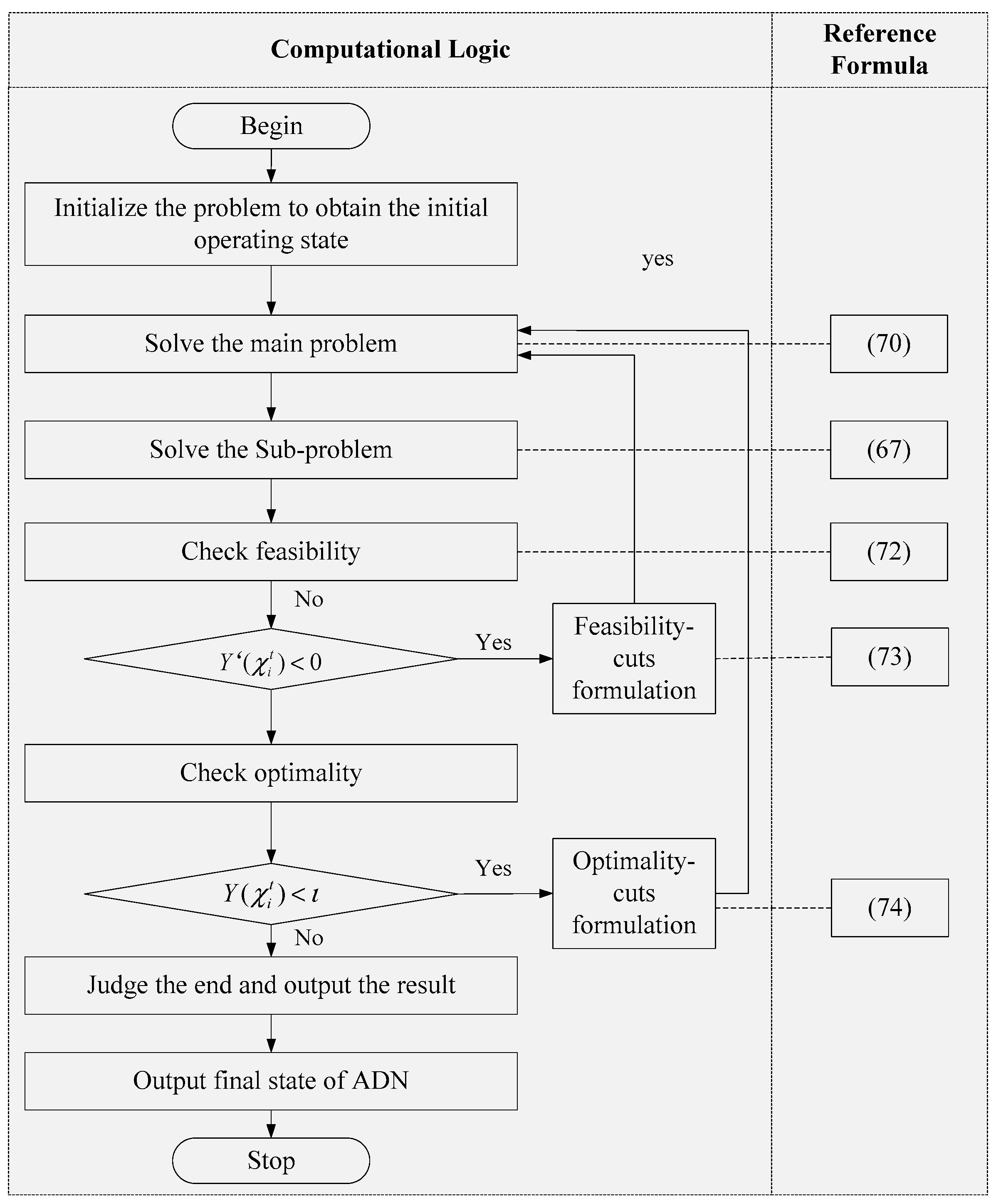
The computational algorithm framework is shown as Figure 1. The core steps include main problem solving, sub-problem solving and constraint set updating.
4. Demonstration Application for Optimal Operation
The demonstration application for active distribution network located in Guizhou, China. The strategy of stochastic optimal operation is verified based on the structure of the demonstration. The schematic diagram for the demonstration project is shown in Figure 2. The distributed generation and flexible load conditions are listed in Table 1. All electric vehicles support vehicle-to-grid (V2G) mode.
The electricity price adopts the peak valley electricity price as Shanghai, the electricity price is ¥0.68 per kWh from 9:00 to 22:00, and electricity price is ¥0.33 per kWh for the rest of the time. is set to ¥0.167 per kWh [25]. The controllable range for HVACs in the demonstration are shown in Figure 3.
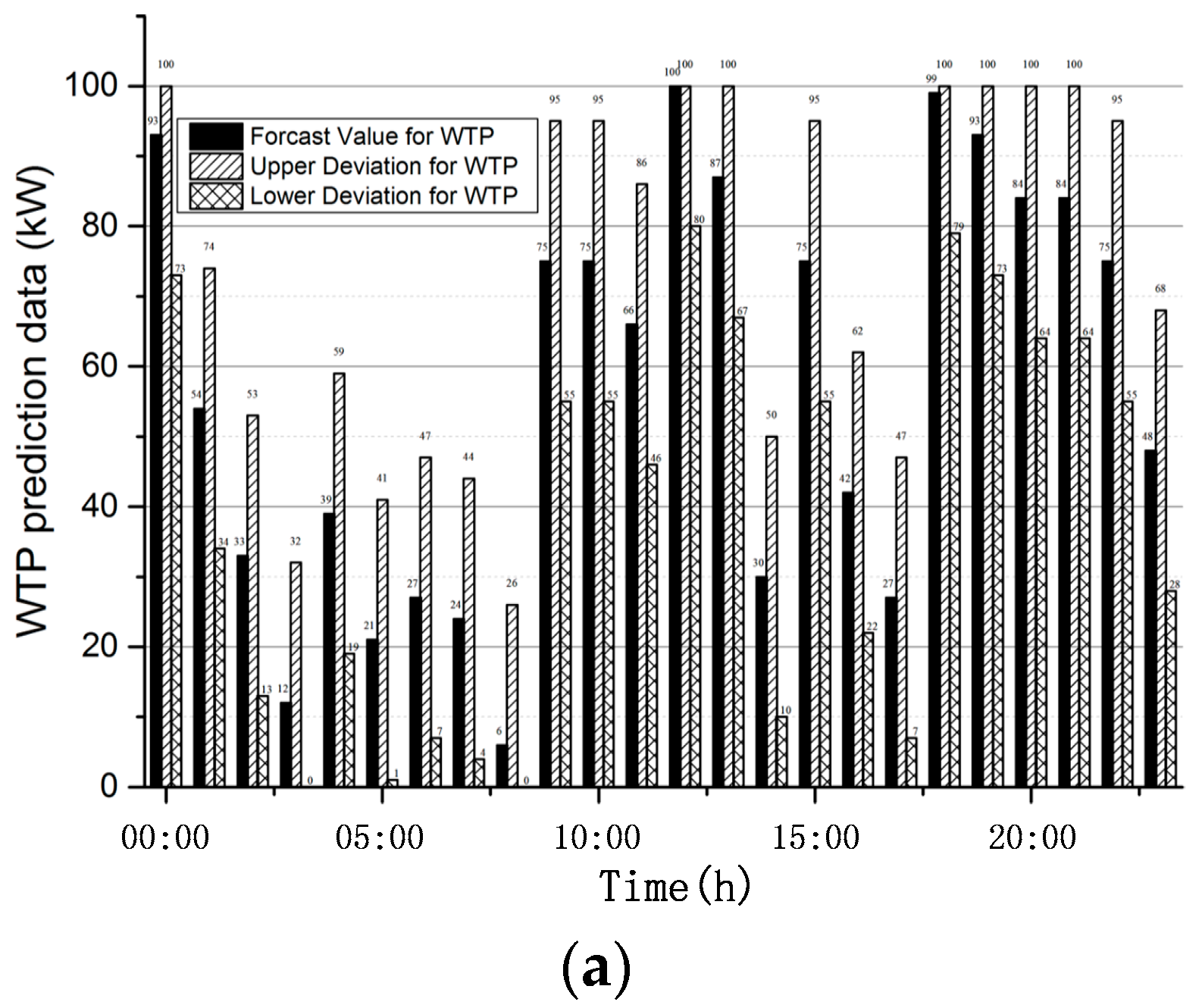
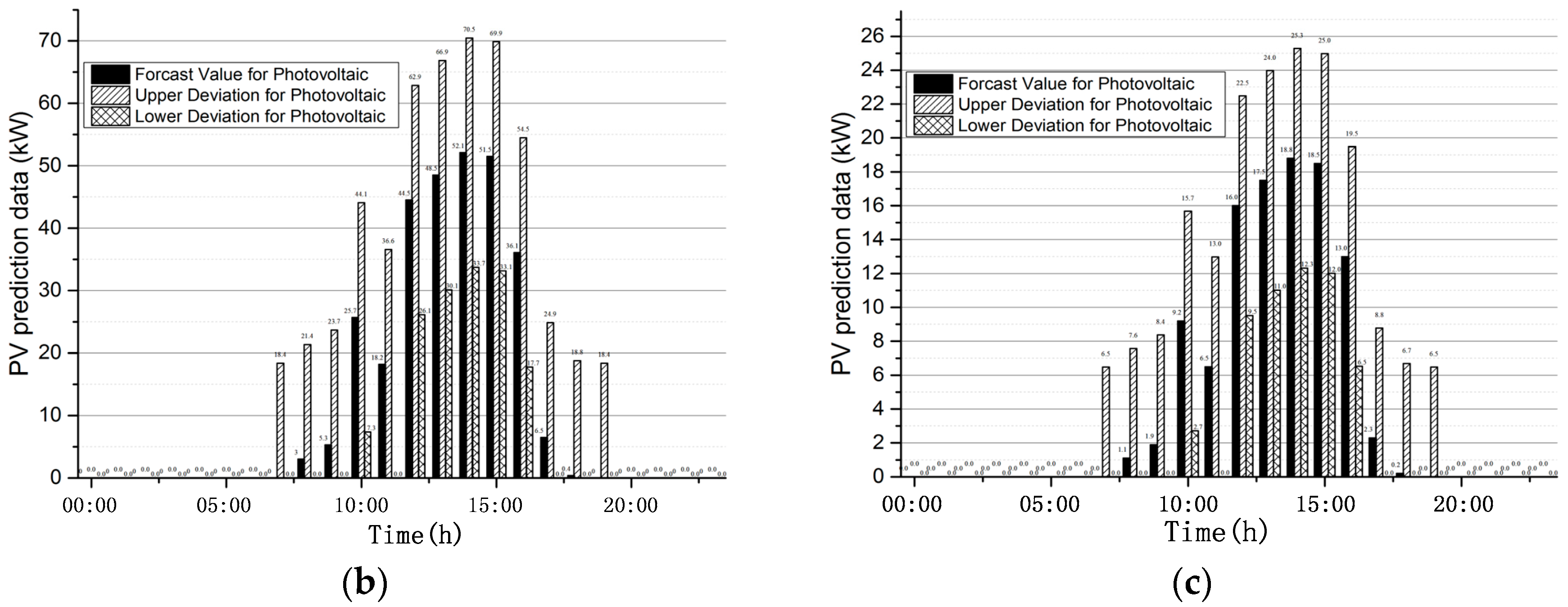
The upper and lower deviations for intermittent energies are shown in Figure 4. It should be noticed that the deviation for photovoltaic during the night is 0, as it is obvious that the photovoltaic system cannot generate electricity during the night.
4.1. Basic Optimization Scenario
The optimization effect for stochastic operation strategy of ADN is firstly discussed under the basic optimization scenario. The weight selection for objective function ( to ) is set as Table 2.
As the benefit brought by controllable devices is significantly higher than the network loss reduce benefit when is close to , we select the weights by the sensitivity of distributed power output to network loss to ensure both the distributed power supply gains and loss benefits are considered simultaneously.
The uncertainty for intermittent energy is set to 8. Table 3 showed the worst case after the solution for intermittent energy. It can be seen that the worst case for intermittent tend to have a negative deviation () when the load is relatively larger and have a positive deviation () when the load is relatively smaller.
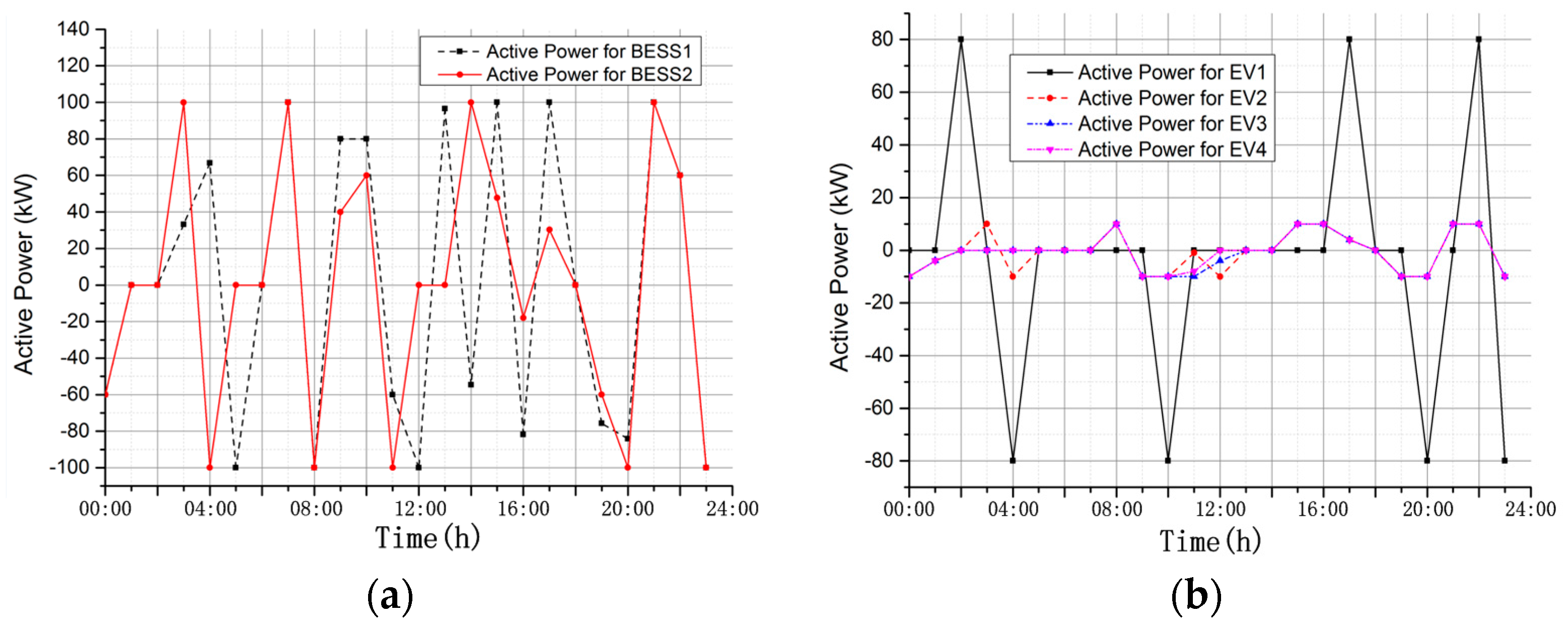
The optimization result for both energy storage devices and power regulation devices are shown in Figure 5 and Figure 6.
It should be noticed that CCHP is connected to the ShuiPei feeder. As the rated power for CCHP is relatively small compared to the load along the feeder, when the active power for CCHP is rising, the benefit for power regulation devices and the benefit for network loss are increasing at the same time, so the active power for CCHP rose to the upper limit as shown in Figure 6a.
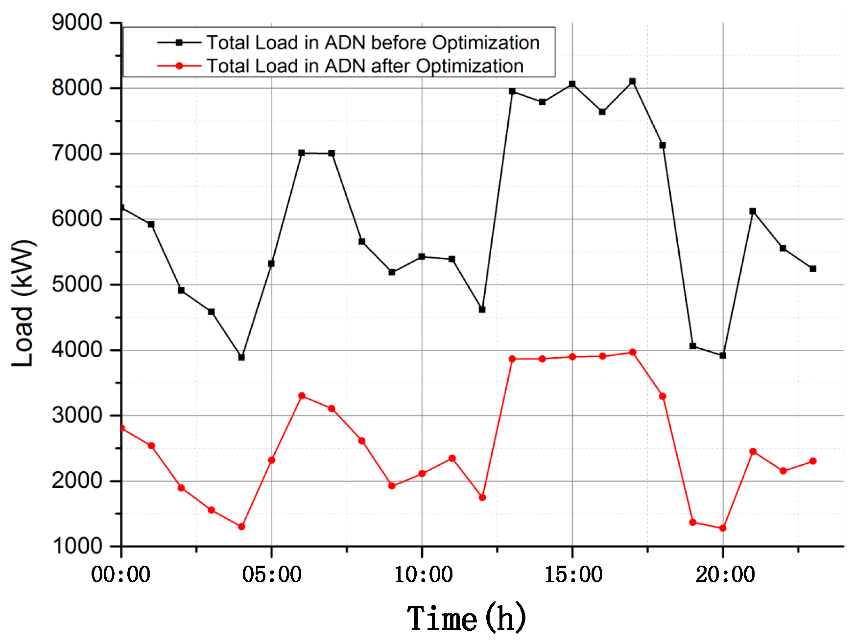
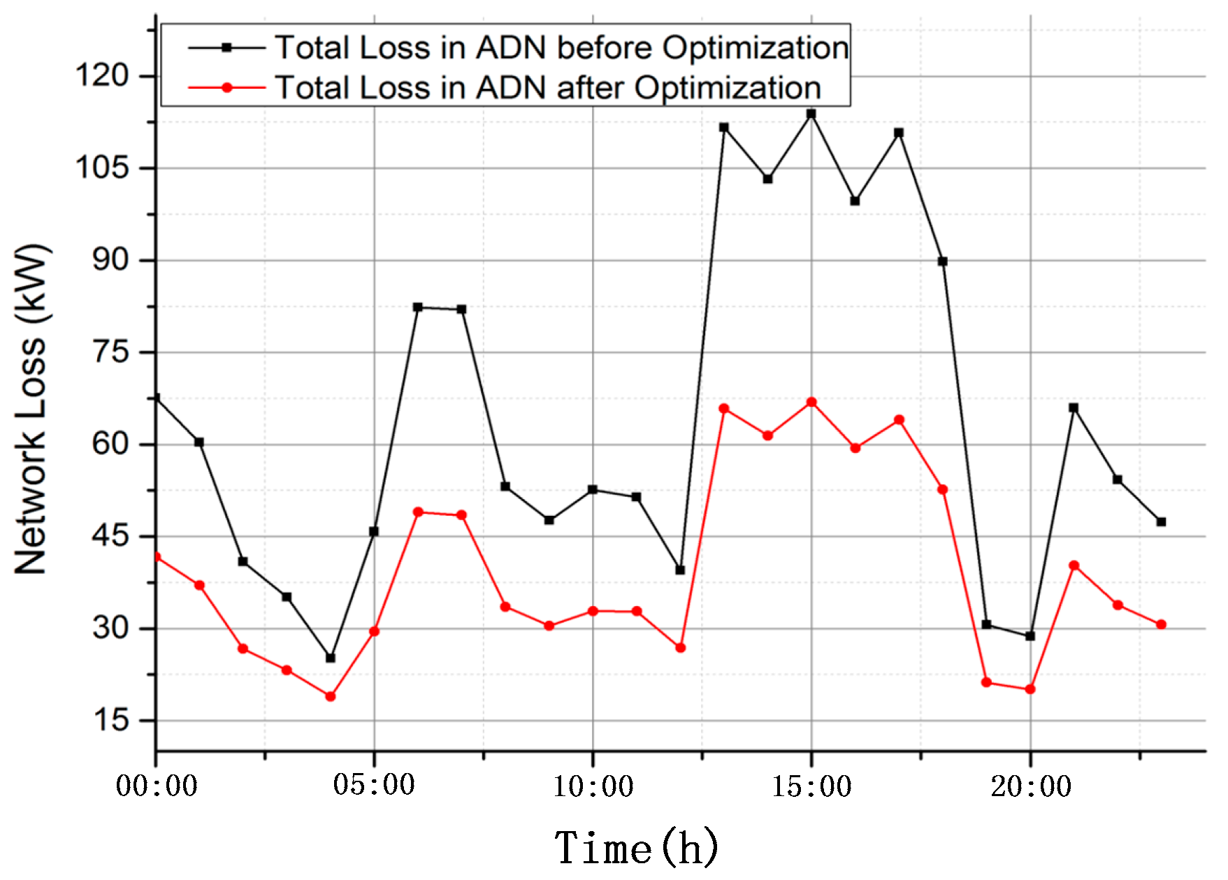
The optimization effects are shown in Figure 7 and Figure 8. The initial state before optimization is recorded as (22a) and (23a). The total load after the optimization is shown as the red line in Figure 7 that has already taken the worst intermittent energy case into consideration. The peak-valley difference has reduced by 1531.36 kW (from 4218.08 kW to 2686.72 kW). The network loss has reduced by 591.689 kW (from 1538.78 kW to 947.091 kW).
Then the influence of both intermittent energy power output uncertainty and the objective function weight selection to the optimization are discussed under different scenarios.
4.2. Different Intermittent Energy Uncertainty
In this part of the paper we select two more representative scenarios where and to discuss the influence of different uncertainty for intermittent energy . represents the number of time intervals when the intermittent energy output reaches the limits or .
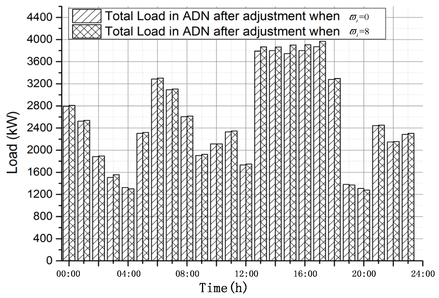
When the active power for all intermittent energy will be strictly the predicted value, which means there is no ‘worst scenario’ for the optimization equlation. Figure 9 shows the different optimization results in ADN when compared to the loads in ADN when . The peak-valley difference is reduced to 2561.18 kW when , which was better than .
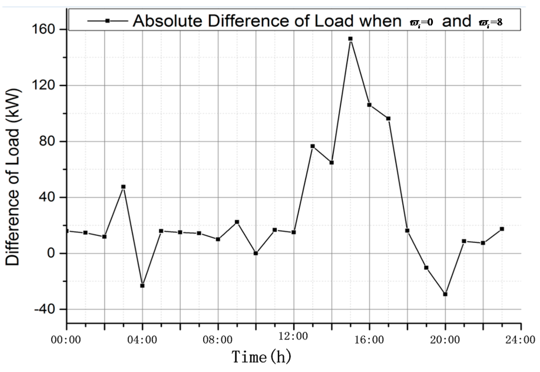
The absolute difference of load is shown in Figure 10 for a more explicit analysis. It can be observed that the time periods when the load difference is relatively large are basically the same periods of intermittent energy prediction uncertainty selection periods.
As the active power for intermittent energy is small, the network loss wouldn’t be influenced that much. The total network loss when is 949.29 kW, which is only a 0.23% difference compared to the network loss when .
When , the intermittent power supply uncertainty has more choices, which will lead to a worse scenario shown in Table 4.
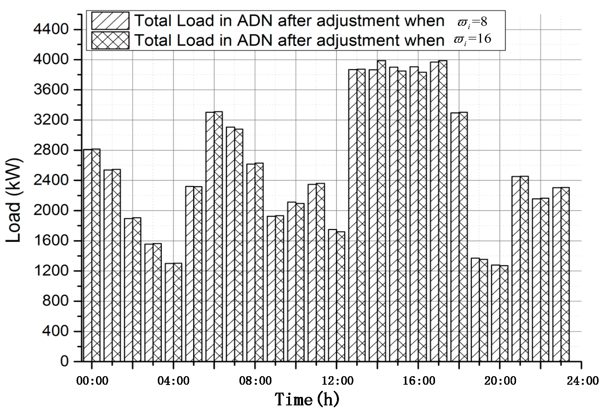
Figure 11 compares the optimization result when with the result when . The peak-valley difference increased to 2714.12 kW, which is the worst among all three scenarios, but the network loss is 945.74 kW, which has only a −0.14% difference compared to the network loss when .
4.3. Different Objective Function Weight Selection
In this part, we will discuss the influence of different objective function weight selections. In all scenarios of this part, is set to 8 to exclude the impact of intermittent energy uncertainty.
The first scenario is set to neglect the benefit of all controllable devices including both energy storage devices and power regulation devices. This scenario happens when all controllable devices are owned by the user, so the benefit of controllable devices does not affect the DSO’s choice of optimization strategy. The weight selection for the objective function is set as in Table 5.
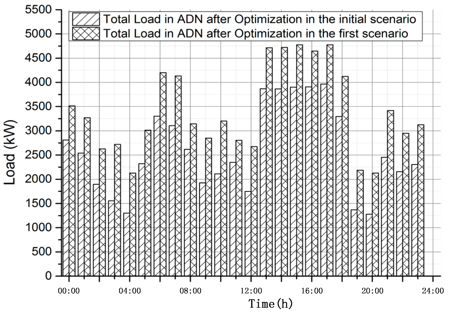
We take the basic optimization scenario discussed in the first part of this section as the initial scenario. The optimization results for total load in ADN is shown in Figure 12.
The peak-valley difference in this scenario is reduced to 2648.93 kW, which is better than the initial scenario. It can be seen from Figure 12 that the total load in ADN in the first scenario is larger than the total load in the initial scenario. That’s because as the benefit brought by controllable devices was neglected, the objective function wouldn’t encourage the output of controllable devices. The network loss comparison is shown in Figure 13. The total network loss reduced from 947.091 kW in the initial scenario to 834.38 kW in this scenario.
The second scenario is set to be more biased in favor of the benefit brought by controllable devices. The weight selection for both and are set to be higher as in Table 6.
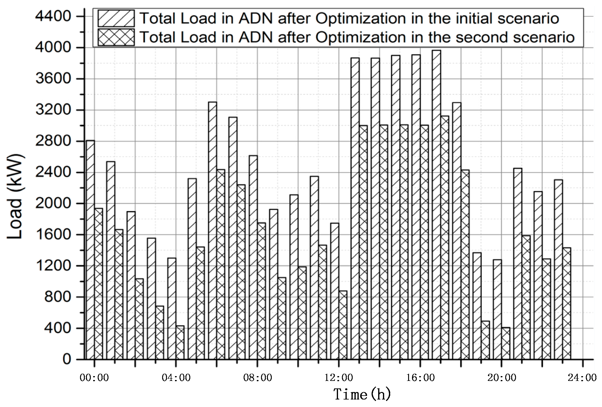
The optimization results for both load and network loss in ADN are shown in Figure 14 and Figure 15.
As the objective function was set to encourage the benefit brought by controllable devices, the active power for controllable devices appears to rise. The total load in ADN decreased as shown in Figure 14. The peak-valley difference in this scenario was increased to 2711.80 kW. The network loss was also increased to 1279.946 kW. The active power for different distributed generations are shown in Figure 16 and Figure 17. The total active power is larger than in the initial scenario.
Based on the former result and discussion, different weight selection will lead to a different optimization effect. In practice, we can flexibly adjust the weight as needed in order to obtain an optimized result.
4.4. Optimization Results Analysis
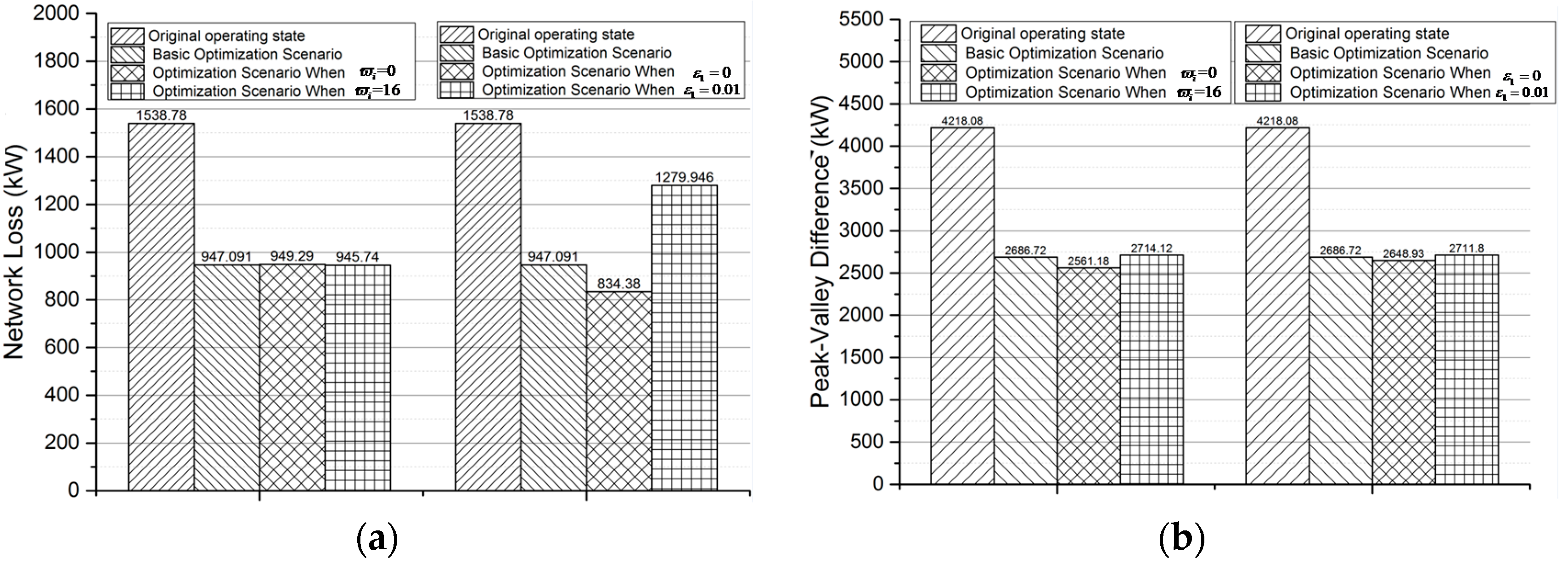
The summary of optimization results for the former scenarios is shown in Figure 18. The optimal operation strategy proposed in this paper realizes an efficient usage of all kinds of controllable resources. It can be seen from the figure that both network losses and the peak-valley differences are improved in all scenarios compared to the original operation state.
The left part of Figure 18a,b show the influence of the intermittent energy uncertainties on the optimization result. The increase of intermittent energy uncertainties will lead to the decrease of the optimization effect, while increasing the compatibility for intermittent energy fluctuations in ADN at the same time.
The right part of Figure 18a,b shows the influence of different objective function weight selection on the optimization results. By adjusting the objective function weight, we can choose to obtain better power grid operation effect or to encourage more distributed power supply.
5. Conclusions
In this paper, we have developed an optimal operation strategy to realize an efficient usage of all kinds of controllable resources in active distribution networks including distributed generations and flexible loads. To decrease the formulation complexity, the models for all resources are summarized as three kinds of devices: intermittent energy, energy storage devices and power regulation devices. Uncertainty for intermittent energy is taken into account in this paper to ensure a high utilization of intermittent energy even under the worst scenario. The prediction error can be flexibly adjusted according to the requirements. Then, we establish an objective function taking two main indicators reflecting the operation state of distribution network into consideration, the peak-valley difference and the network loss. We can set the weight of optimization objection to realize different objective function selection. The mathematical equations are reformulated to a two-stage max-min problem. The Benders decomposition algorithm is used in this paper to solve the nonlinear programming problem. Finally, the robustness of the strategy is verified in the demonstration application project for ADN located in Guizhou, China. The simulation is performed under different simulation settings to ensure an optimal operation for ADN. However, in all demand side loads only the controllable loads are taken into consideration in this paper. In further research we will take both demand responses (such as price incentives) and direct load control as responsible resources to realize comprehensive optimization for both active control resources and passive response resources.
Acknowledgments
This work was supported by the National Natural Science Foundation of China: 51677116.
Author Contributions
The paper was a collaborative effort between the authors. The authors contributed collectively to the theoretical analysis, modeling, simulation, and manuscript preparation.
Conflicts of Interest
The authors declare no conflict of interest.
Nomenclature
| ADN | Active Distribution Network |
| SUC | Stochastic Unit Commitment |
| MILP | Mixed-integer Linear Programming |
| HVAC | Heating, Ventilation and Air Conditioning |
| TCL | Thermostatically Controlled load |
| ESS | Energy Storage System |
| SOC | Status of Charge |
| V2G | Vehicle-to-Grid |
| DSO | Distribution System Operator |
| Sets | |
| Set of power regulation devices | |
| Set of energy storage devices | |
| Set of intermittent energy | |
| Set of all buses | |
| Set of all feeders | |
| Parameters | |
| Time periods in optimization horizon, in this paper the horizon is to be 24 h | |
| Time span for optimization, in this paper each time span is to be one hour | |
| Output for power regulation device in time period | |
| Output for energy storage device in time period | |
| Equivalent output for energy storage device in time period | |
| Output for intermittent energy in time period | |
| Rated capacity for energy storage device in time period | |
| Rated power for energy storage device in time period | |
| Rated power for power regulation device in time period | |
| Forecasted output for intermittent energy in time period | |
| Upper deviation for intermittent energy in time period | |
| Lower deviation for intermittent energy in time period | |
| , | Binary decision variables represent the status of deviation for |
| Ramp-up limit for power regulation device | |
| Ramp-down limit for power regulation device | |
| Minimum power limit for power regulation device | |
| Maximum power limit for power regulation device | |
| Initial state of charge (SOC) for energy storage device in optimization horizon | |
| Final state of charge (SOC) for energy storage device in optimization horizon | |
| State of charge (SOC) for energy storage device at the start of time period | |
| Maximum state of charge for energy storage device | |
| Minimum state of charge for energy storage device | |
| Electricity price in time period | |
| Profit for peak-valley regulation per kWh | |
| Peak-valley difference in optimization horizon | |
| , | Initial state and optimized state for peak-valley difference |
| Network loss in time period | |
| , | Initial state and optimized state for network loss in time period |
| Load in time period | |
| Voltage for bus in time period | |
| Transmission current for feeder in time period | |
| , | Extra variables for peak-valley difference calculation |
References
- Weng, J.; Liu, D.; Luo, N.; Tang, X. Distributed processing based fault location, isolation, and service restoration method for active distribution network. J. Mod. Power Syst. Clean Energy 2015, 3, 494–503. [Google Scholar] [CrossRef]
- Ling, W.; Liu, D.; Yang, D.; Sun, C. The situation and trends of feeder automation in China. Renew. Sustain. Energy Rev. 2015, 50, 1138–1147. [Google Scholar] [CrossRef]
- Yu, W.; Liu, D.; Huang, Y. Operation Optimization Based on the Power Supply and Storage Capacity of an Active Distribution Network. Energies 2013, 6, 6423–6438. [Google Scholar] [CrossRef]
- Siahkali, H.; Vakilian, M. Stochastic unit commitment of wind farms integrated in power system. Electr. Power Sys. Res. 2010, 80, 1006–1017. [Google Scholar] [CrossRef]
- Zheng, Q.P.; Wang, J.; Liu, A.L. Stochastic Optimization for Unit Commitment—A Review. IEEE Trans. Power Syst. 2015, 30, 1913–1924. [Google Scholar] [CrossRef]
- Wang, X.; Hu, Z.; Zhang, M.; Hu, M. Two-stage stochastic optimization for unit commitment considering wind power based on scenario analysis. In Proceedings of the 2016 China International Conference on Electricity Distribution (CICED), Xi’an, China, 10–13 August 2016; pp. 1–5. [Google Scholar]
- Hu, B.; Wu, L.; Marwali, M. On the robust solution to SCUC with load and wind uncertainty correlations. IEEE Trans. Power Syst. 2014, 29, 2952–2964. [Google Scholar] [CrossRef]
- Falsafi, H.; Zakariazadeh, A.; Jadid, S. The role of demand response in single and multi-objective wind-thermal generation scheduling: A stochastic programming. Energy 2014, 64, 853–867. [Google Scholar] [CrossRef]
- Mogo., J.B.; Kamwa, I.; Cros, J. Multi-area security-constrained unit commitment and reserve allocation with wind generators. In Proceedings of the 2016 IEEE Canadian Conference on Electrical and Computer Engineering (CCECE), Vancouver, BC, Canada, 15–18 May 2016; pp. 1–6. [Google Scholar]
- Zhao, C.; Guan, Y. Data-Driven Stochastic Unit Commitment for Integrating Wind Generation. IEEE Trans. Power Syst. 2016, 31, 2587–2596. [Google Scholar] [CrossRef]
- Xiang, H.; Ye, S.; Zhao, C.; Wu, M.; Ming, J.; Dai, C. Hierarchical multi-objective unit commitment optimization considering negative peak load regulation ability. In Proceedings of the 2016 China International Conference on Electricity Distribution (CICED), Xi’an, China, 10–13 August 2016; pp. 1–5. [Google Scholar]
- Bavafa, F.; Niknam, T.; Azizipanah-Abarghooee, R.; Terzija, V. A New Bi-Objective Probabilistic Risk Based Wind-Thermal Unit Commitment Using Heuristic Techniques. IEEE Trans. Ind. Inform. 2016, 13, 115–124. [Google Scholar] [CrossRef]
- Wu, Z.; Zeng, P.; Zhang, X.P.; Zhou, Q. A Solution to the Chance-Constrained Two-Stage Stochastic Program for Unit Commitment with Wind Energy Integration. IEEE Trans. Power Syst. 2016, 31, 4185–4196. [Google Scholar] [CrossRef]
- Arora, V.; Chanana, S. A modified approach to solution of Unit Commitment problem using Mendel’s GA method. In Proceedings of the 2016 2nd International Conference on Advances in Electrical, Electronics, Information, Communication and Bio-Informatics (AEEICB), Chennai, India, 27–28 February 2016; pp. 287–291. [Google Scholar]
- Datta, D.; Dutta, S. A binary-real-coded differential evolution for unit commitment problem. Int. J. Electr. Power Energy Syst. 2012, 42, 517–524. [Google Scholar] [CrossRef]
- Yuan, X.; Nie, H.; Su, A.; Wang, L.; Yuan, Y. An improved binary particle swarm optimization for unit commitment problem. Expert Syst. Appl. 2009, 36, 8049–8055. [Google Scholar] [CrossRef]
- El-Zonkoly, A.M. Multistage expansion planning for distribution networks including unit commitment. IET Gener. Transm. Distrib. 2013, 7, 766–778. [Google Scholar] [CrossRef]
- Castillo, A.; Laird, C.; Silva-Monroy, C.A.; Watson, J.P.; O’Neill, R.P. The Unit Commitment Problem with AC Optimal Power Flow Constraints. IEEE Trans. Power Syst. 2016, 31, 4853–4866. [Google Scholar] [CrossRef]
- Han, D.; Jian, J.; Yang, L. Outer approximation and outer-inner approximation approaches for unit commitment problem. IEEE Trans. Power Syst. 2014, 29, 505–513. [Google Scholar] [CrossRef]
- Zeng, B.; An, Y.; Kuznia, L. Chance constrained mixed integer program: Bilinear and linear formulations, and Benders decomposition. Mathematics 2014, 3, 1–30. [Google Scholar]
- Nasri, A.; Kazempour, S.J.; Conejo, A.J.; Ghandhari, M. Network-Constrained AC Unit Commitment under Uncertainty: A Benders’ Decomposition Approach. IEEE Trans. Power Syst. 2016, 31, 412–422. [Google Scholar] [CrossRef]
- Chen, F.; Liu, D.; Li, Q. Active Load Management Strategy Considering Fluctuation Characteristics of Intermittent Energy. In Proceedings of the 23rd International Conference on Electricity Distribution (CIRED’15), Lyon, France, 15–18 June 2015; pp. 1–5. [Google Scholar]
- Zhao, C.; Wang, J.; Watson, J.P.; Guan, Y. Multi-stage robust unit commitment considering wind and demand response uncertainties. IEEE Trans. Power Syst. 2013, 28, 2708–2717. [Google Scholar] [CrossRef]
- Santos, T.N.; Diniz, A.L. Feasibility and optimality cuts for the multistage Benders decomposition approach: Application to the network constrained hydrothermal scheduling. In Proceedings of the Power & Energy Society General Meeting, 2009 (PES’09), Calgary, AB, Canada, 26–30 July 2009; pp. 1–8. [Google Scholar]
- Zhang, J.; Cheng, H.; Wang, C.; Xia, Y.; Shen, X.; Yu, J. Quantitive assessment of active management of distribution network with distributed generation. In Proceedings of the Third International Conference on Electric Utility Deregulation and Restructuring and Power Technologies (DRPT 2008), Nanjing, China, 6–9 April 2008; pp. 2519–2524. [Google Scholar]
Figure 1.
Framework for computational algorithm based on Benders’ decomposition.

Figure 2.
Demonstration Project of ADN located in Guizhou, China.
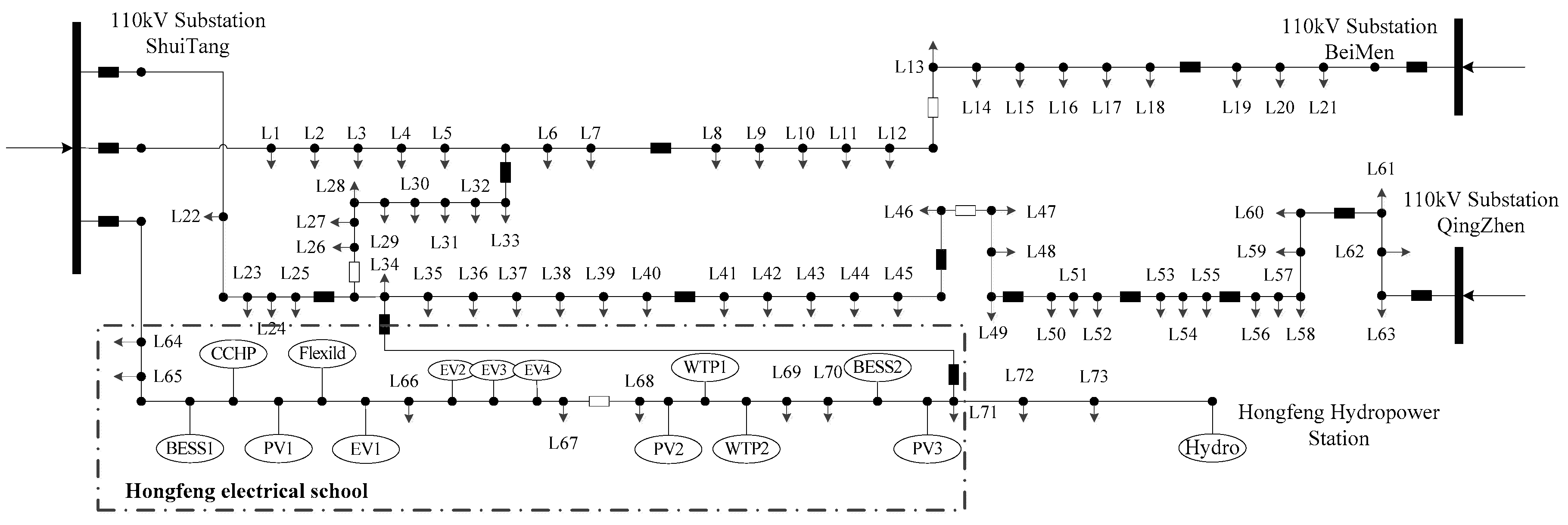
Figure 3.
Controllable Range for HVACs.
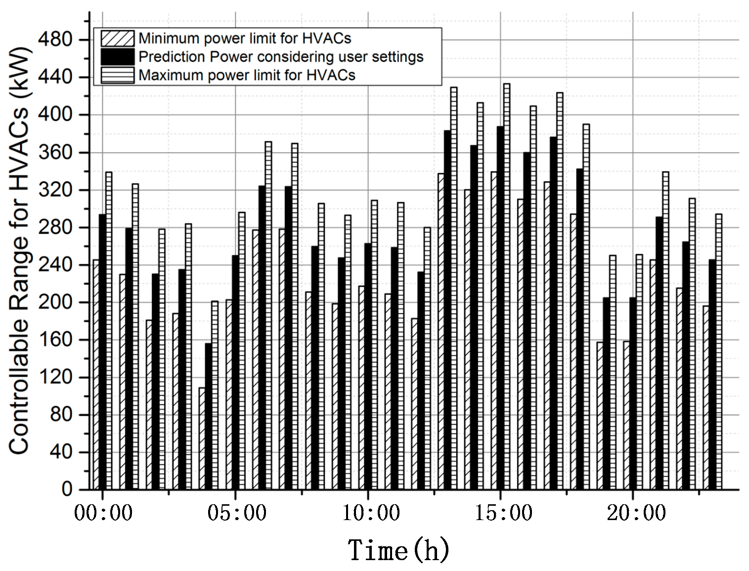
Figure 4.
Forecast Value Deviation for Intermittent Energies: (a) Power Deviation for WTP1 and WTP2; (b) Power Deviation for PV2&4; (c) Power Deviation for PV1&3.
Figure 4.
Forecast Value Deviation for Intermittent Energies: (a) Power Deviation for WTP1 and WTP2; (b) Power Deviation for PV2&4; (c) Power Deviation for PV1&3.


Figure 5.
Optimization result for energy storage devices: (a) Active Power for BESS; (b) Active Power for EV.
Figure 5.
Optimization result for energy storage devices: (a) Active Power for BESS; (b) Active Power for EV.

Figure 6.
Optimization result for power regulation devices: (a) Active Power for CCHP and Hydro; (b) Active Power for Flexild.
Figure 6.
Optimization result for power regulation devices: (a) Active Power for CCHP and Hydro; (b) Active Power for Flexild.
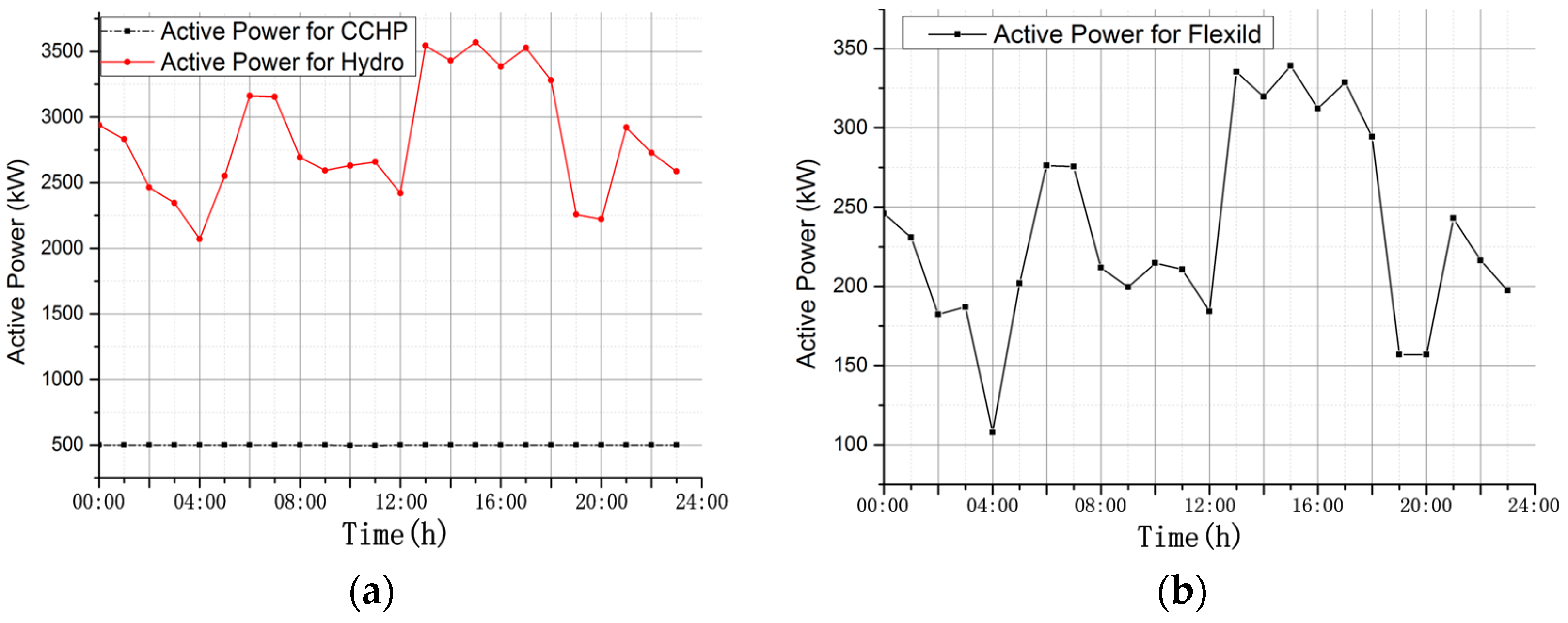
Figure 7.
Load comparison before and after optimization.

Figure 8.
Network loss comparison before and after optimization.

Figure 9.
Load comparison when and .

Figure 10.
Absolute error of load when and .

Figure 11.
Load comparison when and .

Figure 12.
Total load comparison for different scenarios.

Figure 13.
Total loss comparison for different scenarios.
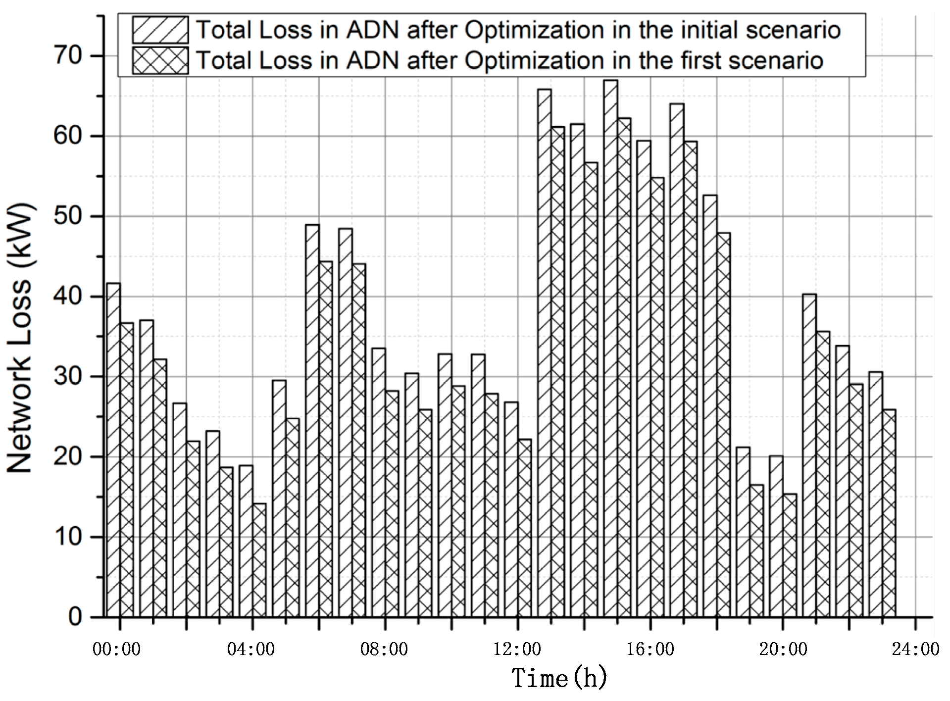
Figure 14.
Total load comparison for different scenarios.

Figure 15.
Total loss comparison for different scenarios.
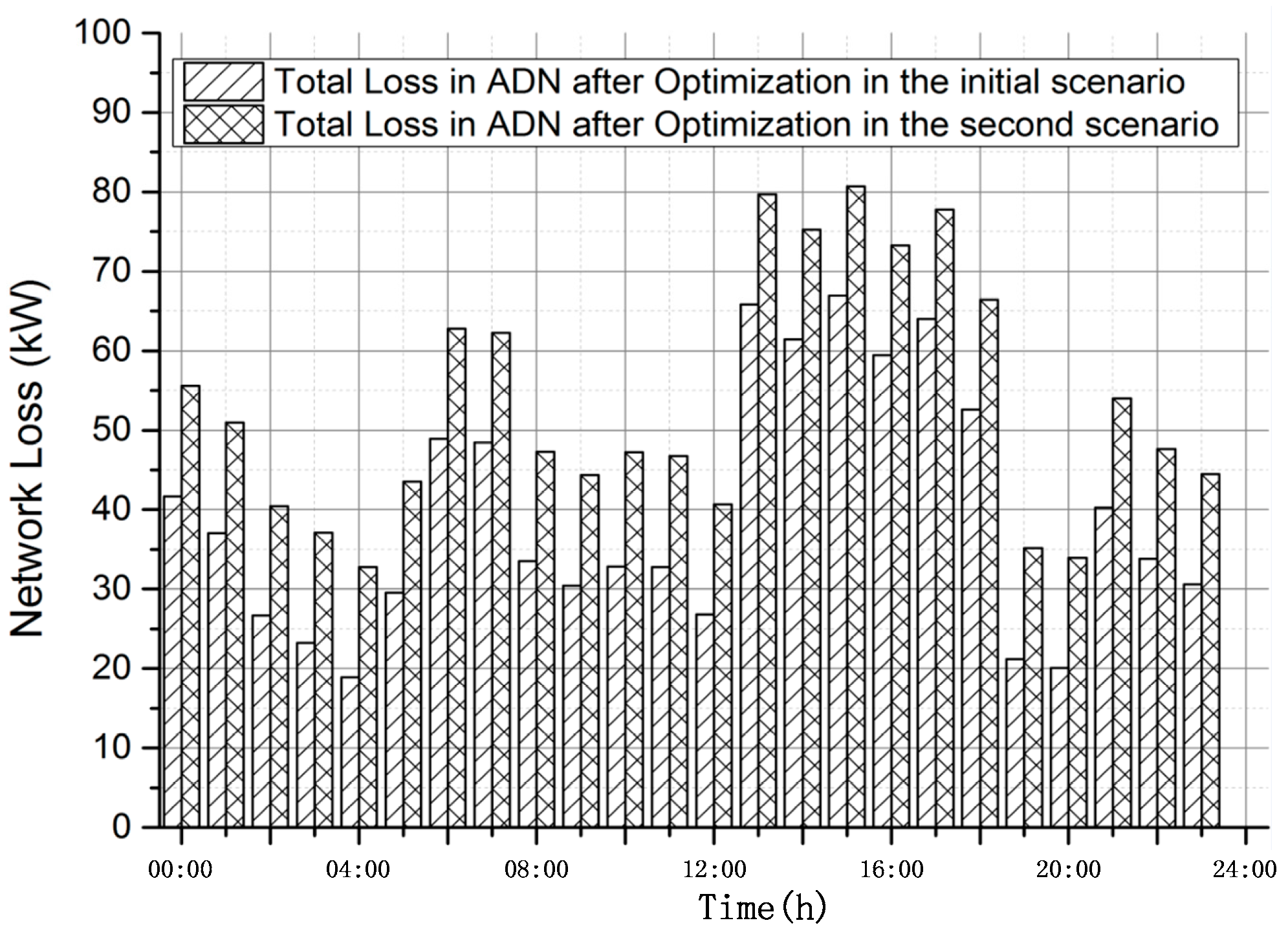
Figure 16.
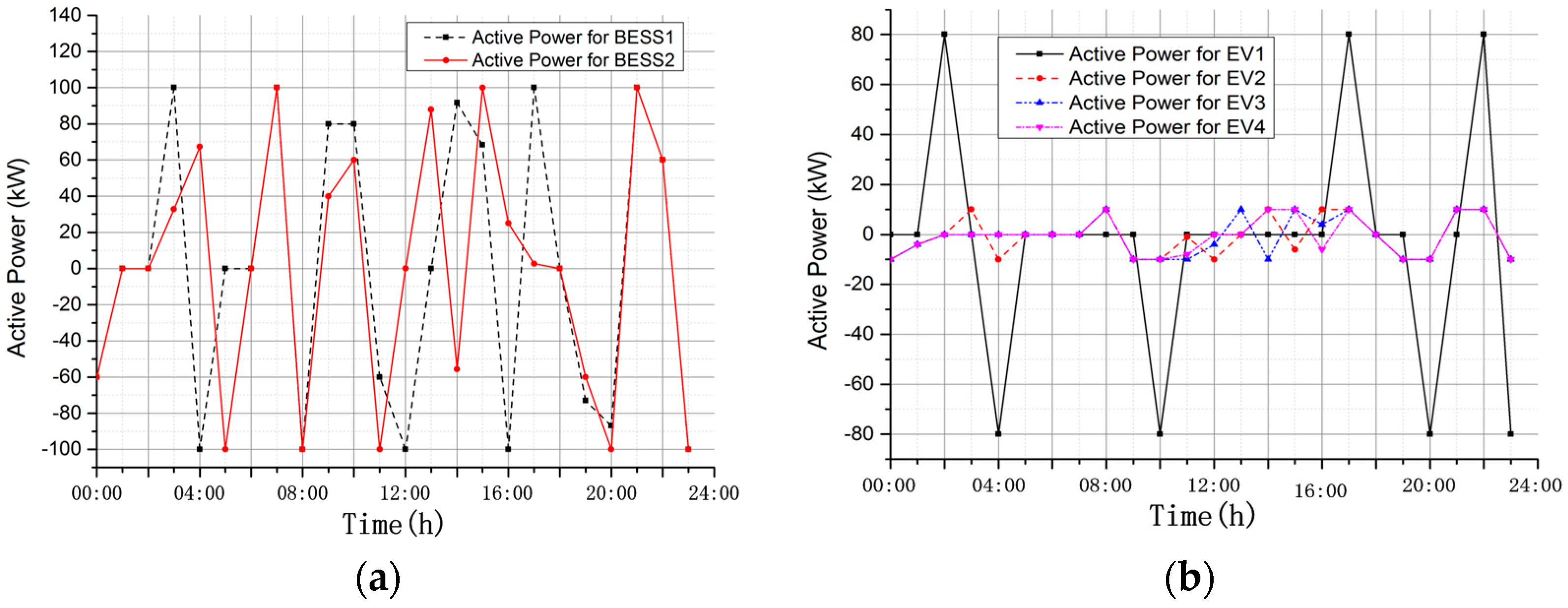
Optimization result for energy storage devices in the second scenario: (a) Active Power for BESS; (b) Active Power for EV.
Figure 16.
Optimization result for energy storage devices in the second scenario: (a) Active Power for BESS; (b) Active Power for EV.

Figure 17.
Optimization result for power regulation devices in the second scenario: (a) Active Power for CCHP and Hydro; (b) Active Power for Flexild.
Figure 17.
Optimization result for power regulation devices in the second scenario: (a) Active Power for CCHP and Hydro; (b) Active Power for Flexild.
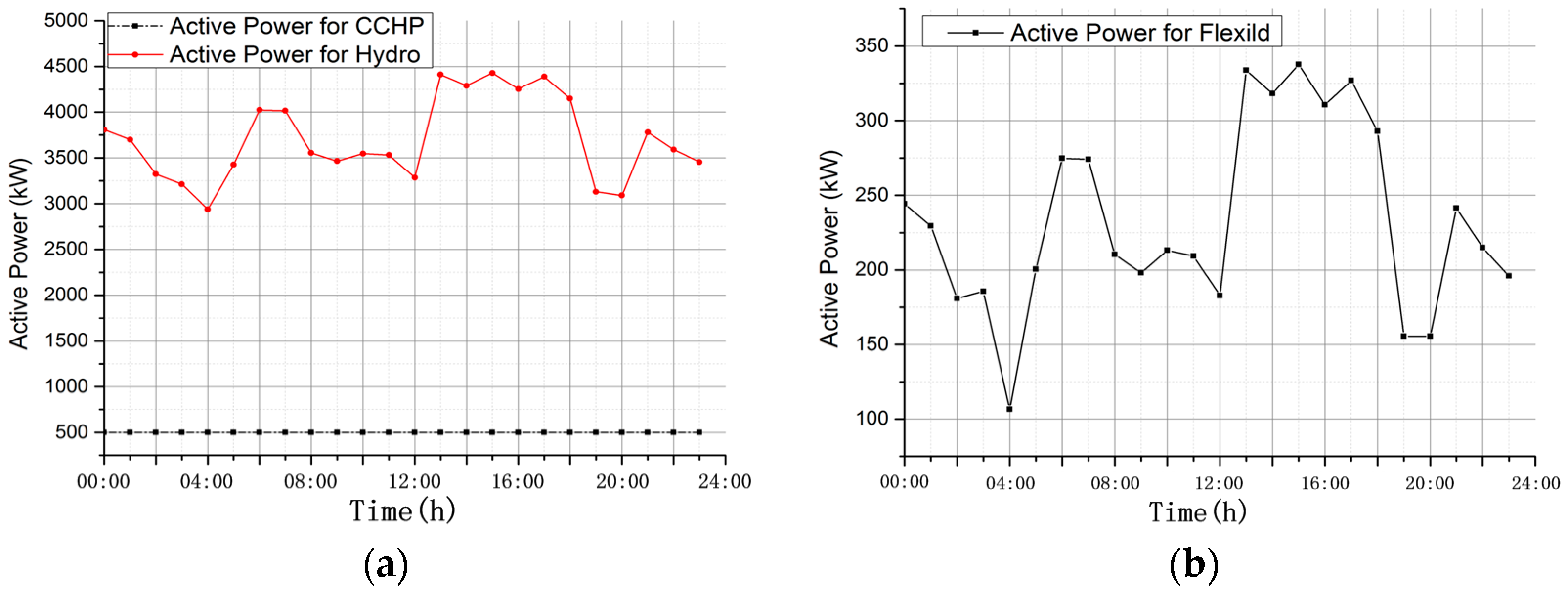
Figure 18.
Summary of Optimization Results. (a) Network Loss Comparison; (b) Peak-valley Difference Comparison.
Figure 18.
Summary of Optimization Results. (a) Network Loss Comparison; (b) Peak-valley Difference Comparison.

Table 1.
Condition for Distributed Generation and Flexible Load in Demonstration Project.
| Name | Types of Devices | Capacity of Devices | |
|---|---|---|---|
| PV1 | Photovoltaic | Intermittent energies | 32.4 kW |
| PV2 | 91.8 kW | ||
| PV3 | 32.4 kW | ||
| PV4 | 91.8 kW | ||
| WTP1 | Wind turbine | 100 kW | |
| WTP2 | 100 kW | ||
| BESS1 | Battery energy storage system | Energy storage devices | 100 kW/200 kWh |
| BESS2 | 100 kW/200 kWh | ||
| EV1 | Electric vehicle | 100 kW/200 kWh | |
| EV2 | 10 kW/30 kWh | ||
| EV3 | 10 kW/30 kWh | ||
| EV4 | 10 kW/30 kWh | ||
| Hydro | Hydropower | 10,000 kW | |
| CCHP | Cooling-heating-power supply | Power regulation devices | 500 kW |
| Flexild | HVAC | ||
Table 2.
Weight Selection for Optimization.
| Name | Weight Selection |
|---|---|
| 0.005 | |
| 0.495 | |
| 0.25 | |
| 0.25 |
Table 3.
Intermittent energy uncertainty when .
| Name | Intermittent Energy Uncertainty | |
|---|---|---|
| Time Period When | Time Period When | |
| PV1 | 19 | 14,15,16,17 |
| PV2 | 19,20 | 13,14,15,16,17,18 |
| PV3 | 19 | 14,16,17 |
| PV4 | 19,20 | 13,14,15,16,18 |
| WTP1 | 19,20 | 13,14,15,16,17 |
| WTP2 | 19,20 | 13,14,15,16,17 |
Table 4.
Intermittent Energy Uncertainty when .
| Name | Intermittent Energy Uncertainty | |
|---|---|---|
| Time Period when | Time Period when | |
| PV1 | 7,10,11,12,19 | 8,9,13,14,15,16,17,18 |
| PV2 | 7,10,12,19 | 8,9,13,14,15,16,17,18 |
| PV3 | 7,10,12,19 | 8,9,13,14,15,16,17,18 |
| PV4 | 7,10,12,19 | 8,9,13,14,15,16,17,18 |
| WTP1 | 19,20 | 13,14,15,16,17 |
| WTP2 | 19,20 | 13,14,15,16,17 |
Table 5.
Weight Selection for Optimization.
| Name | Weight Selection |
|---|---|
| 0 | |
| 0.5 | |
| 0 | |
| 0.5 |
Table 6.
Weight Selection for Optimization.
| Name | Weight Selection |
|---|---|
| 0.01 | |
| 0.49 | |
| 0.375 | |
| 0.125 |
© 2017 by the authors. Licensee MDPI, Basel, Switzerland. This article is an open access article distributed under the terms and conditions of the Creative Commons Attribution (CC BY) license (http://creativecommons.org/licenses/by/4.0/).
Share and Cite
MDPI and ACS Style
Chen, F.; Liu, D.; Xiong, X. Research on Stochastic Optimal Operation Strategy of Active Distribution Network Considering Intermittent Energy. Energies 2017, 10, 522. https://doi.org/10.3390/en10040522
AMA Style
Chen F, Liu D, Xiong X. Research on Stochastic Optimal Operation Strategy of Active Distribution Network Considering Intermittent Energy. Energies. 2017; 10(4):522. https://doi.org/10.3390/en10040522
Chicago/Turabian StyleChen, Fei, Dong Liu, and Xiaofang Xiong. 2017. "Research on Stochastic Optimal Operation Strategy of Active Distribution Network Considering Intermittent Energy" Energies 10, no. 4: 522. https://doi.org/10.3390/en10040522
Note that from the first issue of 2016, this journal uses article numbers instead of page numbers. See further details here.