An Optimized Home Energy Management System with Integrated Renewable Energy and Storage Resources

Abstract

Traditional power grid and its demand-side management (DSM) techniques are centralized and mainly focus on industrial consumers. The ignorance of residential and commercial sectors in DSM activities degrades the overall performance of a conventional grid. Therefore, the concept of DSM and demand response (DR) via residential sector makes the smart grid (SG) superior over the traditional grid. In this context, this paper proposes an optimized home energy management system (OHEMS) that not only facilitates the integration of renewable energy source (RES) and energy storage system (ESS) but also incorporates the residential sector into DSM activities. The proposed OHEMS minimizes the electricity bill by scheduling the household appliances and ESS in response to the dynamic pricing of electricity market. First, the constrained optimization problem is mathematically formulated by using multiple knapsack problems, and then solved by using the heuristic algorithms; genetic algorithm (GA), binary particle swarm optimization (BPSO), wind driven optimization (WDO), bacterial foraging optimization (BFO) and hybrid GA-PSO (HGPO) algorithms. The performance of the proposed scheme and heuristic algorithms is evaluated via MATLAB simulations. Results illustrate that the integration of RES and ESS reduces the electricity bill and peak-to-average ratio (PAR) by 19.94% and 21.55% respectively. Moreover, the HGPO algorithm based home energy management system outperforms the other heuristic algorithms, and further reduces the bill by 25.12% and PAR by 24.88%.

1. Introduction

In recent decades, energy demand around the globe has shown the increasing trend. In past, most of the power generation was being done from fossil fuels. However, to fulfil the increasing electricity demand with minimal emissions of green house gases scientists have worked on the new means of electricity generation: renewable and sustainable energy resources (RSERs). But, the penetration of renewable energy sources (RESs) significantly increased power system complexity and dynamics [1], and the existing power system is not capable of maintaining its stability if the integration of RESs and distributed generation (DG) is done at a large scale. In this context, one of the present solutions is the transformation of the existing power grid into the smart grid (SG) with cutting edge information and communication technologies (ICTs) [2]. These advanced ICTs not only enable SG to incorporate the DG and RESs but also enhance the stability and reliability of power system. European technology platform (European Commission, 2006) defines the SG as, “a smart grid is an electricity network that can intelligently integrate the actions of all users connected to it-generators, consumers and those that do both in order to efficiently deliver sustainable, economic and secure electricity supplies”. SG has different kinds of operational and energy measures like smart meters (SMs), smart appliances, renewable energy and electric energy storage resources. The vital aspect of SG is the control of power production, transmission and distribution through advanced ICTs. These ICTs enable SG to send control commands within the time limits defined by numerous international standards e.g., IEEE standards 1547 (i.e., the standards defined for the control and management of distributed energy resources) [3]. Moreover, SG makes possible the access of the power system operator and end-users at the same time intelligently and efficiently.

The key factors that make SG superior over traditional grids are: two-way communication, advanced metering infrastructure (AMI) and information management units (IMUs). They introduce intelligence, automation and realtime control to power system. The two-way communication in SG not only keeps the end-users well informed about the varying electricity prices, maintenance schedules of the distribution network and events/failures that come either due to equipment failures or natural disasters but also enables the operator to monitor and analyze the realtime data of energy consumption and makes realtime decision about the operation activities and standby generators. A comprehensive comparison of traditional grid and SG features is shown in

Table 1. A brief comparison of traditional grid and smart grid (SG).

Infrastructure	Traditional Grid	SG
Power system	Centralized generation. Uni-directional flow of energy from utility to the consumers.	Decentralized generation. Two-way flow of energy between the utility and the prosumers.
Power Losses	High power losses due to centralized structure and inadequate storage facilities.	Significantly reduces the power losses due to DG at distribution level (i.e., the DG eliminates the losses of transmission network).
Information system	Aged metering and monitoring system	Advanced metering and monitoring system: AMI and supervisory control and data acquisition system (SCADA)
Communication system	Wired technology	Both wired and wireless technologies
ESSs	Main storage facility is pump-hydro power plants.	Facilitate the distributed ESSs integration
RSERs	Mainly includes dispatchable RESs (Hydro-power plants)	Provides decentralized control for RSERs (solar, wind, tidal, geo-thermal and biomass energies etc.)
Self-healing	Reacts to stop further damage. Emphasis is on protection of assets following system faults.	Automatically senses and reacts to actual and emerging contingencies. Focus is on prevention.
Optimization of assets	Negligible incorporation of limited operational data with assets management processes and technologies. Time based maintenance.	Greatly expanded sensing and measurement of grid conditions, grid technologies deeply integrated with assets management processes to effectively manage assets and costs. Condition based maintenance.
Consumer engagement	No proper involvement of the consumers in DSM and DR activities (i.e., no mechanism to send the varying electricity prices to the consumers in realtime and forced load shedding is carried out to maintain the balance between demand and supply)	Provides dynamic pricing, net metering and other incentive based schemes.
Power Quality	Focus only on the reduction of failures and interruptions.	Ensure the quality of electricity for the smooth operations of sensitive electronics devices/equipments.

.

The SG makes the integration of RESs and DGs practicable and involves the residential and commercial users into demand-side management (DSM) and demand response (DR) activities [4]. DSM is the modification of consumer demand for energy through various methods such as financial incentives and behavioral change through education. Usually, the goal of DSM is to encourage the consumers to use less energy during peak hours, or to move the time of energy use to off-peak hours [5]. DSM techniques are used to optimize energy consumption pattern, to efficiently utilize the limited energy resources and to enhance the overall efficiency of the power system. The term DR is used for the programs designed to encourage end-users to make short-term reductions in energy demand in response to a price signal from the electricity hourly market, or a trigger initiated by the electricity grid operator. It is a change in the power consumption of an electric utility consumer to better match the demand for power with the supply. DR seeks to adjust the demand for power instead of adjusting the supply. However, it is totally impractical to ask the consumers to schedule their energy usage by compromising their comfort level. Therefore, an automatic home energy management system (HEMS) is required, however, a little awareness of consumers is required to know the benefits of various scheduling schemes. In this context, we present an OHEMS which not only integrates RES and ESS into residential sector but also incorporate residential consumers into DSM activities.

The common objectives of different DSM and DR strategies in SG are the reduction of the electricity cost and minimization of energy consumption in peak hours. To achieve these objectives numerous algorithms for an efficient HEMS have been proposed, such as integer linear programming (ILP) [6], mixed integer linear programming (MILP) [7], multi-parametric programming [8], etc. However, these techniques cannot tackle a large range of various household appliances having unpredictable, non-linear and complicated energy usage patterns.

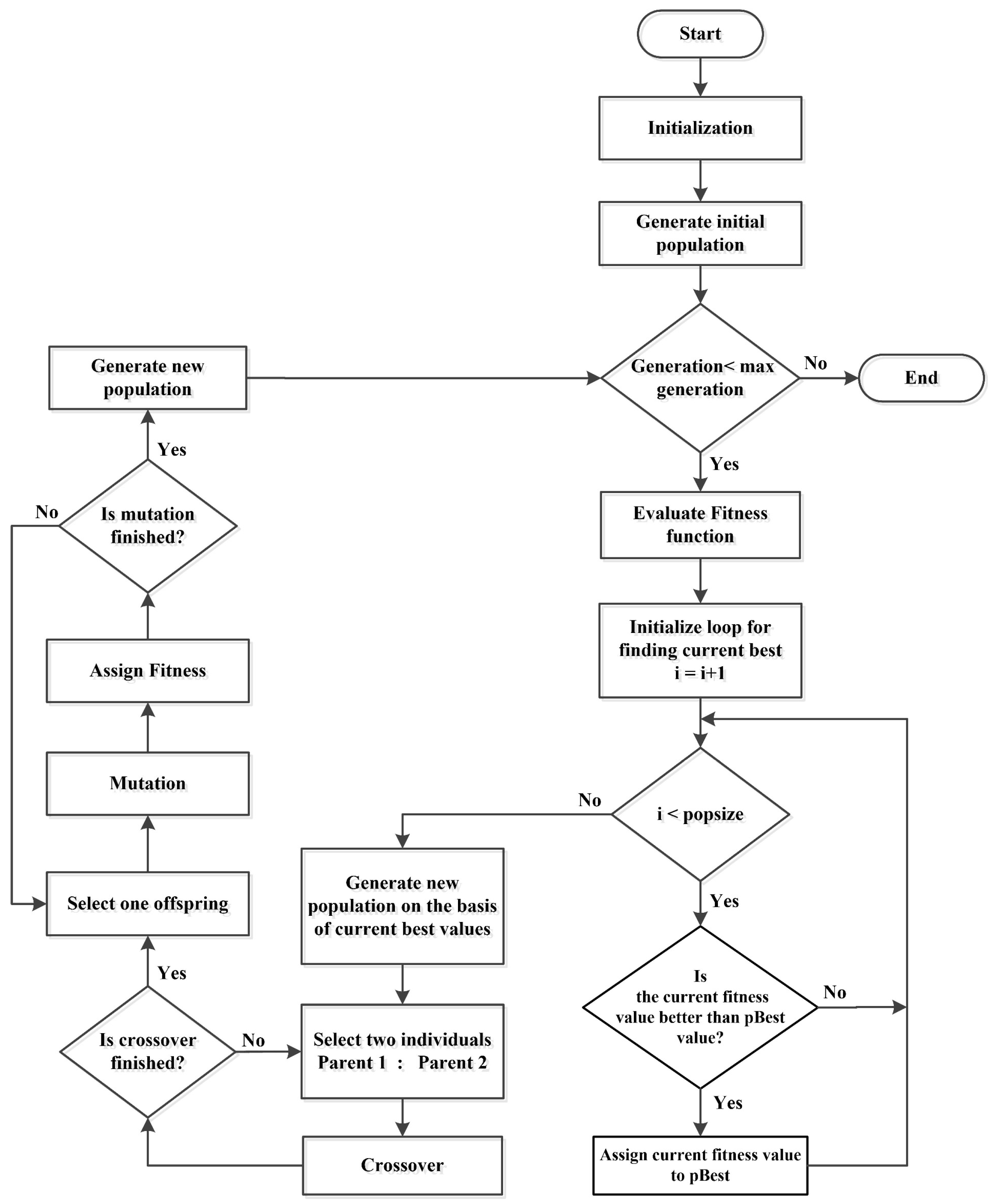
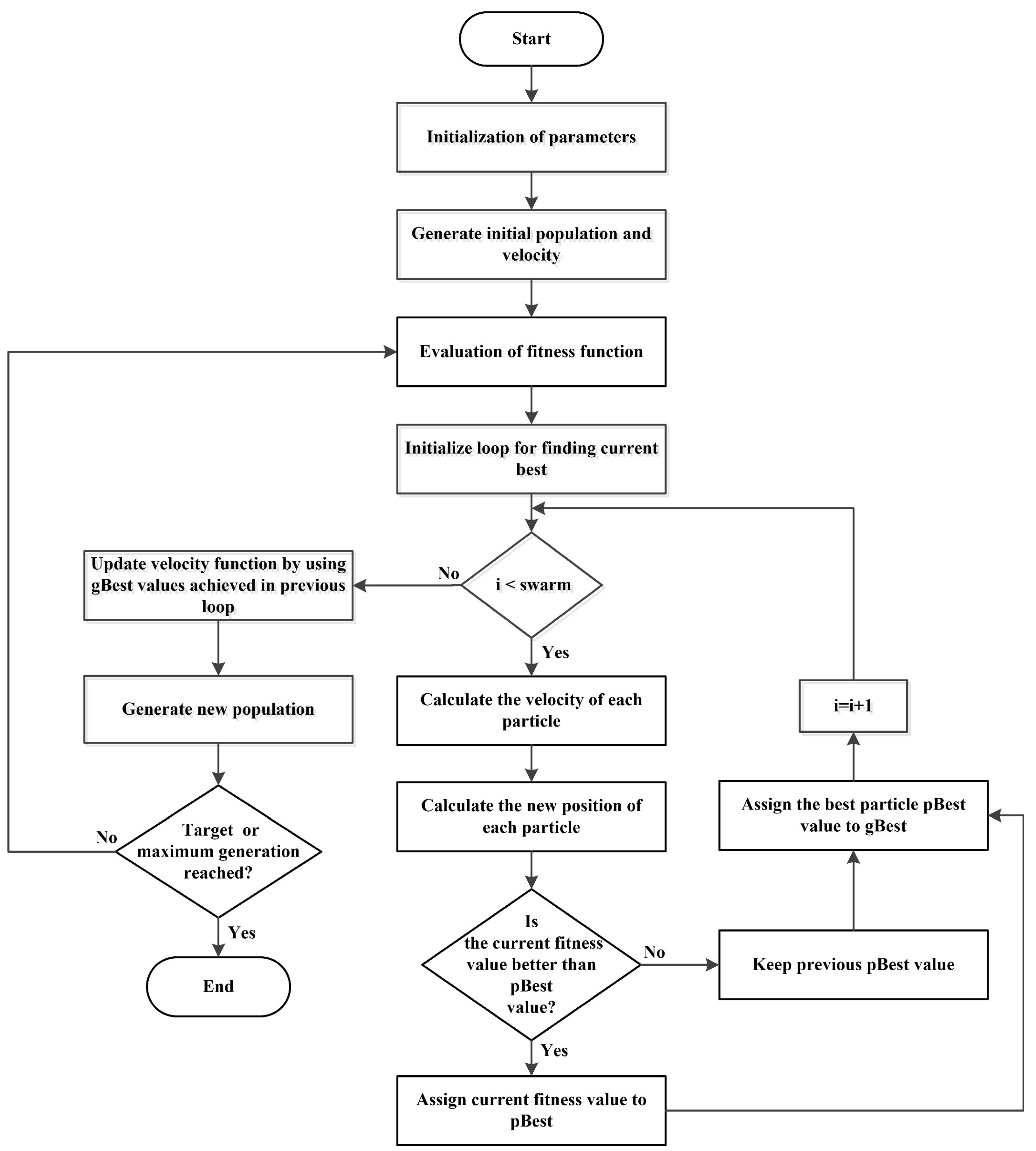
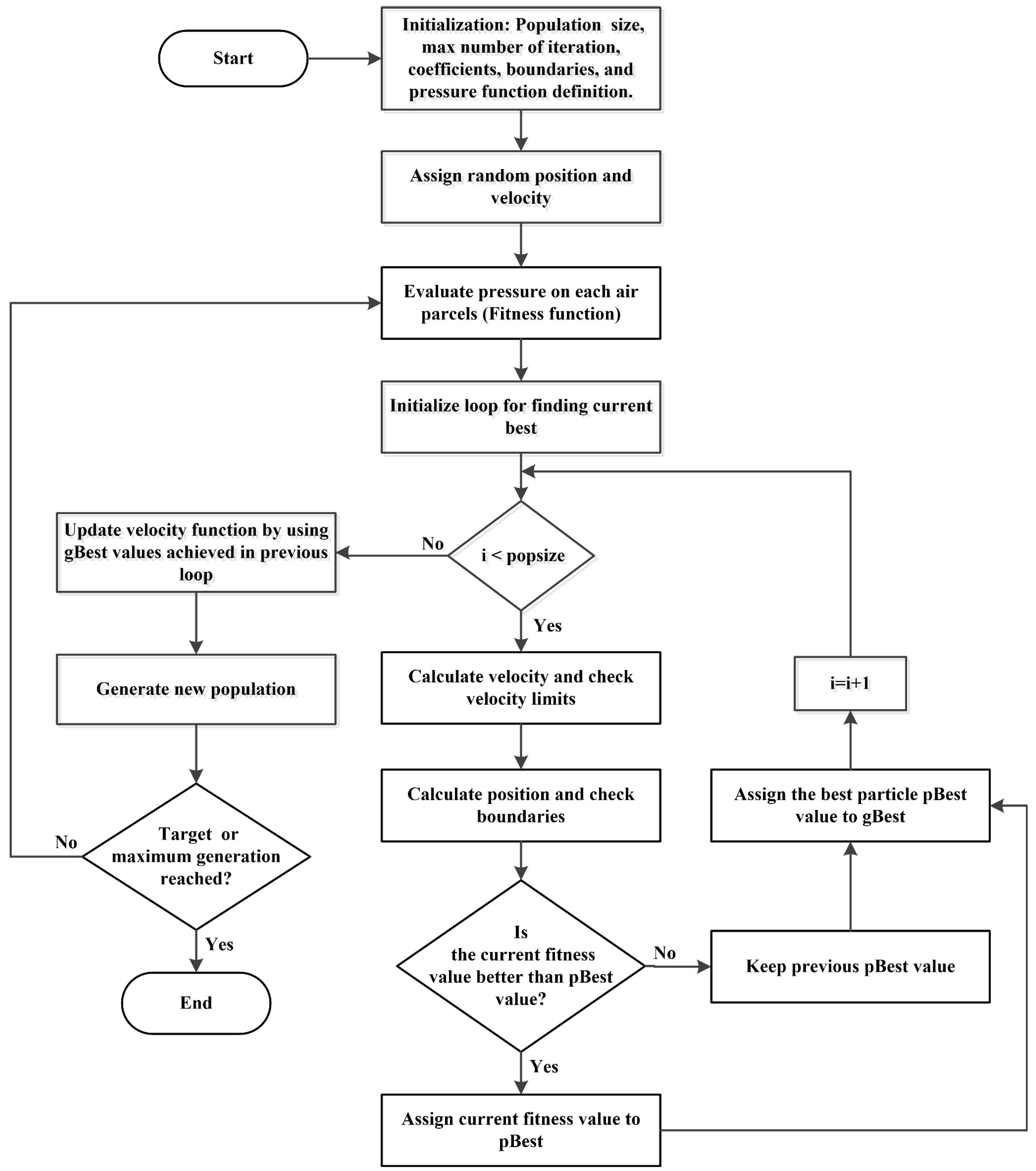
To overcome the deficiencies of the previously proposed HEMSs, this paper presents an optimized home energy management system (OHEMS). The proposed scheme not only facilitates the integration of RES and ESS into the residential sector but also reduces the prosumer’s electricity bill as well as the PAR. In addition, the performance of the heuristic algorithms: genetic algorithm (GA), binary particle swarm optimization (BPSO), wind driven optimization (WDO), bacterial foraging optimization (BFO) and hybrid GA-PSO (HGPO) are also evaluated in terms of energy consumption pattern, and electricity bill as well as PAR minimization. First, an energy management system (EMS) is designed using exogenous grid signals; day-ahead pricing (DAP) signal, ambient temperature, and solar irradiance. Then, the heuristic algorithms are applied to get an optimum solution for the formulated objective function. The adequacy of proposed OHEMS is validated via simulations. The simulations are conducted in two stages, in the first case, the benefits of RES and ESS integration are highlighted, while in the second case the performance of GA, BPSO, WDO, BFO and HGPO algorithms based HEMSs is compared in terms of electricity bill and PAR reduction, and uniform distribution of energy consumption patterns.

The rest of the paper is organized as follows. Section 2 and Section 3 briefly describe the related work and problem statement respectively. Section 4 deals with problem formulation. Section 5 and Section 6 present the proposed system architecture and algorithms respectively. Results and discussions are presented in Section 7, and the paper is concluded in Section 8.

2. Related Work

Recently, numerous DSM strategies have been proposed. Their common objectives are the minimization of electricity cost, reduction of PAR, mitigation of carbon emissions, and enhancement of power system efficiency. The appliances scheduling problem has been solved as an optimization problem by numerous classical and heuristics algorithms. In this context, some of the recent studies are given below, and a brief review of some state of the art trends is presented in

Table 2. Recent Trends: State of the art.

Technique	Domain	Desired Objective	Findings	Remarks
LP [16]	REMS	Reduction of electricity bill and PAR	Objectives are achieved via charging ESS from grid in off-peak hours and then discharging it in peak hours	RES has not been utilized
ILP [17]	Appliances scheduling and integration of RES	Reduction of electricity bill and peak load	A significant reduction bill and peak loads is achieved via RES integration and optimizing energy consumption pattern	UC and ESS is not considered
MILP [18]	HEMS, and integration as well as grid interconnection of RES	Reduction of cost and PAR via RES utilization	Cost reduction is achieved	Infeasible for small scale residential consumers
LSA-ANN, and PSO-ANN [19]	HEMS, and appliances scheduling	Cost reduction and comparison of LSA-ANN and PSO-ANN	LNA-ANN outperformed the PSO-ANN, and significantly reduce the electricity bill	UC and PAR reduction is not considered
PSO, WDO, and K-WDO [20]	Appliances scheduling	Minimization of electricity cost and maximization of UC	A favorable trade-off between the cost and UC is achieved, and K-WDO performs better than other algorithms	RES is not exploited
RL [21]	Fully-automated EMS	Optimization of appliances operating time, and reduction of PAR	Peaks formation is avoided, and cost reduction is achieved	UC and RES is not considered
GA [22]	REMS	Electricity cost and PAR reduction	New peaks formation is avoided by dividing the appliances into clusters	UC is compromised, and RES is not considered
GA, and PSO [23]	Appliances scheduling	Optimization of appliances operating time to pay minimum electricity bill	GA-based scheduling achieves the desired objectives with less computational cost and efforts	UC is compromised at achieving the minimum electricity bill
GA [24]	HEMS	Reduction of electricity bill and PAR	Hybrid of RTP and ToUP is ued to avoid the peaks formation	UC is not considered
Greedy iterative algorithm [25]	EMS, and optimization of grid operation	Optimization of consumers energy consumption pattern for grid station stability	RTP signal is used an invisible hand to optimized the energy consumption pattern	UC is compromised
IPSO [26]	Grid station stability	Reduction of load in peak hours	The desired objective is achieved by rejecting extra load requests in peak hours	Only passive appliances are considered, and UC is compromised.

.

In [9], the authors present a review of current trends in HEMS and DR in the residential sector. The importance of HEMS for relocating and curtailment of the load is also discussed. They give insights on existing optimization techniques: mathematical optimization, model predictive control and heuristics algorithms. The impact of forecasting uncertainty, devices heterogeneity, computational limitation and timing consideration in the design of optimization algorithms are also discussed. However, the user comfort (UC) and appliances waiting time have not been discussed. The authors in [10], present a compact survey of the current trends in HEMS. The challenges in the implementation of HEMS are discussed and give the insights on current literature regarding DR, DSM, appliance scheduling, and on single or multiple objective optimizations in HEMS. However, the integration of RESs and ESSs into residential sector, their impacts on electricity bill and PAR have not been addressed.

In [11], the authors discussed the importance of energy management and planning in smart cities (SC). The paper presents a review on the planning and optimization of SC energy system. Four areas of SC energy system: generation, storage, transportation and end user are addressed in detail. Although, an ESS is integrated to supports residential load in grid events. But, the scheduling of appliances or relocating of load and ESS in response to dynamic pricing of electricity market has not been discussed. The authors in [12], give insights regarding the ways and manners that facilitate the integration of RESs and DG in the SG and the concept of SCs have been comprehensively addressed. The obstacles to the integration of DG into the existing distribution network have been highlighted. The effect of DG on voltage stability and control at low and medium voltages are also discussed. Moreover, the impact of DG on power quality, power system stability, and related events of voltage sag and swell due to the failure of distributed sources are addressed in a comprehensive way. Although, the authors discussed the impact of DGs and RESs integration on power quality and power system stability. However, the integration of RESs and ESSs into residential sector and their role in DSM programs have been ignored.

In [13], the authors present a detailed review of evaluating trends in smart homes (SHs) and SG. They investigate the effectiveness of various communication technologies: Zig-Bee, Z-Wave, Wi-Fi and wired protocols. The authors point out the merits and demerits of existing technologies, and products available in the market. Moreover, the barriers, challenges, benefits, and future trends regarding the communication technologies and their role in the SG and SHs are also discussed. The authors in [14], demonstrate a residential energy monitoring system (REMS). Three SHs powered by an in-house RES (i.e., PV system) are considered for demonstration. The SH is equipped with data logger system to measure and record the electricity production and demand patterns. The internal and external temperature, as well as the humidity is recorded to accurately schedule the operation of heating ventilation and air conditioning (HVAC) system. However, this paper did not address the integration of ESS to utilize the RE more efficiently.

A. Mehmood et al. [15], present an in-depth review of load furcating (LF), current LF techniques in existing power system, future trends, and its importance for the implementation of future SG is discussed. They elaborate the two major types of LF: mathematical modelling and artificial intelligence based computational models and their subcategories as well. The authors also present a comparative study of various dynamic pricing schemes: realtime pricing (RTP), Time of Use pricing (ToUP) and critical peak pricing(CPP).

Lee et al. [16], present linear programming (LP) based REMS for reduction of electricity cost and PAR by charging the ESS from utility in off-peak hours and is discharged in peak hors. The integration of RESs into residential sector is not considered and the charging of ESS from utility is not an economical solution. In [17], the authors propose an ILP based HEMS with integrated RES for appliances scheduling to shift the shiftable appliances from peak hours to off-peak hours. However, the authors did not consider the UC and ESS integration. The authors in [18], discuss the scheduling of home appliances for designed objective of electricity cost minimization or optimization of electricity consumption pattern. MILP is used to schedule the household appliances and the RES. An in-house RES not only reduces the electricity bills but the surplus energy is also sold to the utility to generate revenue. Although, RES with HEMS is fruitful for both the utility and the prosumer, however, the installation of RES may not be feasible for a single/small domestic consumer.

In [19], the authors proposed a hybrid technique of lighting search algorithm (LSA) and artificial neural network (ANN) to generate an optimal operation patterns of the appliances. Four appliances are modeled and developed in MATLAB/SIMULINK, with pre-defined preferences of the consumer. To optimize the appliances ON/OFF time, and to complete the assigned tasks with minimum cost, a hybridization of LSA and ANN is used. The proposed technique significantly reduces the electricity cost and outperforms the hybrid of particle swarm optimization (PSO) based ANN. However, RES and ESS has not been taken into account to more efficiently minimize the electricity bill. In addition, the reduction of PAR and its impact on power system has not been discussed.

A comparative study of WDO and PSO is done in [20]. Household appliances are considered for scheduling with the objectives of cost minimization and UC maximization. Moreover, Knapsack-WDO (K-WDO) is also studied for the same objective functions. Results illustrate that K-WDO perform better than WDO and PSO. However, in the proposed model the integration of RES is not considered and an ESS is used to store energy from grid in off-peak hours which is not a viable solution.

Z. Weng et al. [21], demonstrate a fully automated energy management system (EMS) using reinforcement learning (RL) techniques. The energy management and appliance scheduling problem is solved by observe, learn and adapt (OLA) algorithm which adds more intelligence to EMS. The proposed mechanism significantly reduce the cost and PAR, but UC is compromised.

In [22], the authors discuss the problem of peak demand during certain hours. The concept of clustering and smart charging has been introduced to maximize the benefits in term of cost reduction and UC. A GA-based EMS is designed which efficiently utilizes energy within the clusters by scheduling the ESS and appliances. Results show that by appropriate scheduling of ESS and appliances in RTP environment customer can get maximum saving over electricity bill. The authors in [23] present the comparison of GA and PSO in terms of computational cost and computational efforts. Results show that PSO needs less computational effort and computational cost to reach an optimal solution as compared to GA. In [24], the authors demonstrate an efficient HEMS architecture for implementation of DSM in the residential sector. They combine RTP scheme with ToUP because the use of only RTP signal may shift the peak demand to off-peak hours. To eliminate the creation of new peaks, an objective function is properly formulated and solved by using GA. Results illustrate that the hybridization of RTP and ToUP schemes is effective for reduction of bill and PAR. Moreover, an acceptable trade-off between the UC and cost reduction is also achieved.

P. Chavali et al. [25], present a distributed mechanism for REMS and grid optimization using the greedy iterative algorithm. In the proposed technique, the electricity price is used as an invisible hand to optimize the appliances scheduling and energy consumption. The proposed scheme did not consider the user comfort in the problem formulation. In [26], the authors proposed an improved-PSO (IPSO) for the solution of cost minimization problem. Results illustrate that the proposed IPSO brings the user load curve near to the objective curve, where the objective curve and electricity price have an inverse relationship. One of the objective functions is power system stability, and the proposed scheme compromise on the UC by rejecting the load in peak hours.

3. Problem Statement

The rapid increase in household electronic appliances significantly increase the electricity demand of residential sector. Almost 40% of the generated electricity is consumed by the residential sector [27]. Currently, power generation is heavily dependent on fossil fuels and the hour of need is to fulfil the inevitably increasing electricity demand with minimal emissions of greenhouse gases. Therefore, scientists have worked to figure out new means of electricity generation i.e., RSERs. In this context, the integration of RSERs and ESSs become lucrative for the researchers. Moreover, the conventional power grid is already vulnerable to instability due to heavy loaded conditions and will be unable to maintain its stability if the integration of RESs is done at a large scale. So, the research is going on to implement the SG in a distributed manner, and HEMS is an integral part of SG to optimize the energy consumption of household appliances. Keeping this objective in mind, we seek to develop an OHEMS. Our objective is twofold: (i) integration of RES and ESS into residential sector; (ii) energy management through appliances and resource scheduling. In order to achieve the above-mentioned objectives, and to design an efficient HEMS, various algorithms such as LP [28], ILP [29], MILP [30], dynamic programming (DP) [31] and convex programming (CP) [32] have been proposed. However, these techniques have very slow convergence rate, and in some cases, they are unable to handle a large number of appliances. So, the heuristic algorithms such as GA [33], BPSO [34], WDO [35] and BFO [36] are introduced to overcome these problems. The heuristic optimizations are used where it is very difficult to find the exact optimal/feasible points. For example, in case of LP, it is understood that the optimal solution must lies within the solutions points in that pool. However, in heuristic optimization, there might be infinite or more solution points in that solution space and optimal solutions should be any one among those. Moreover, in the aforementioned techniques (LP, ILP, MILP, DP and CP) based HEMSs, the integration of RESs, maximization of UC and adaptability with dynamic pricing are ignored. Therefore, in this paper, not only the heuristic algorithms (GA, BPSO, WDO, BFO, and HGPO) are used to design an OHEMS but their performance is also evaluated in terms of energy consumption pattern, electricity bill and PAR reduction.

4. Problem Formulation

In this section, the mathematical models and constraints of photovoltaic (PV) system, ESS and appliances are presented. Based on these descriptions, the optimization problem is formulated.

4.1. Energy Generation Model of PV System

The house of our smart prosumer is equipped with a rooftop PV system (i.e., RES). Although, the RSERs mainly include solar, wind, tidal, geothermal, biomass, and biogass energies, however, among them the most abundant and almost free of cost (i.e., having small operation and maintenance costs) is solar energy and is available everywhere and to everyone. According to [37], the Earth receives 174,000 terawatts (TW) of incoming solar radiation at the upper atmosphere. Approximately 30% is reflected back to space while the rest is absorbed by clouds, oceans and land masses. Most of the world’s population live in areas with insolation levels of 150–300 watts/m${}^2$ or 3.5–7.0 kWh/m${}^2$ per day. In this regard, the proposed OHEMS tries to maximize the benefits from PV system and to minimize the electricity bill, carbon emissions and PAR. The output power $E^{PV}\left(t\right)$ of PV system in kW at time t is calculated by Equation (1) [38],

$$E^{PV}\left(t\right)={\eta }^{PV}·A^{PV}·I_r\left(t\right)·\left(1-0.005(T^a\left(t\right)-25)\right)\forall t$$

(1)

where, ${\eta }^{PV}$ is energy conversion efficiency of the PV system (%), $A^{PV}$ is the area of the generator $\left({\mathrm{m}}^2\right)$, $I_r\left(t\right)$ is the solar irradiance $(\mathrm{k}\mathrm{W}/{\mathrm{m}}^2)$ at time t, $0.005$ is temperature correction factor [39], $T^a\left(t\right)$ is the outdoor temperature (${}^{\circ }\mathrm{C}$) at time t and 25 is standard room temperature (${}^{\circ }\mathrm{C}$). The distribution of hourly sun irradiation usually complies with a bimodal distribution that can be considered as a linear blend of two unimodal distribution functions. The unimodal distribution functions could be modeled by Weibull probability density function as shown in Equation (2) [38,

$$f\left(I_r\left(t\right)\right)=\zeta \left(\frac{{\alpha }_1}{{\beta }_1}\right){\left(\frac{I_r\left(t\right)}{{\beta }_1}\right)}^{({\alpha }_1-1)}{e}^{-{\left(\frac{I_r}{{\beta }_1}\right)}^{{\alpha }_1}}+(1-\zeta )\left(\frac{{\alpha }_2}{{\beta }_2}\right){\left(\frac{I_r\left(t\right)}{{\beta }_2}\right)}^{({\alpha }_2-1)}{e}^{-{\left(\frac{I_r}{{\beta }_2}\right)}^{{\alpha }_2}},0<I_r\left(t\right)<\infty$$

(2)

where, $\zeta$ is a weighted factor, ${\alpha }_1$ and ${\alpha }_2$ are shape factors, together with ${\beta }_1$ and ${\beta }_2$ which are scale factors.

4.2. Energy Storage Model

A small capacity ESS is used to store a portion of electricity generated by PV system, it is mainly for exploiting the PV energy more efficiently. The ESS stores the energy only when its storage level is lower then upper charge level. Electricity stored in the ESS at time t is presented by Equation (3) [38], and the electricity charged, the electricity discharged and the self-discharging rate is taken into account. The charging and discharging of ESS would lose some electrical energy, so turn-around efficiency of ESS is considered.

$$ES\left(t\right)=ES(t-1)+\kappa ·{\eta }^{ESS}·E{P}^{Ch}\left(t\right)-\frac{\kappa ·E{P}^{Dch}\left(t\right)}{{\eta }^{ESS}}\forall t$$

(3)

where $ES$ is stored energy (kWh) at time t, $\kappa$ is time slot duration (hour), ${\eta }^{ESS}$ is ESS efficiency, $E{P}^{Ch}$ is the electric power (kW) supplied to ESS from RES at time and $E{P}^{Dch}$ is is the electric power (kW) supplied to the load from ESS at time t.

In order to maintain the storage and avoid overcharging/deep discharging, charge and discharge rate of electricity, and energy stored in ESS should not exceed the limits defined by the manufacturer.

$$E{P}^{Ch}\left(t\right)\le E{P}_{UB}^{Ch}$$

(4)

$$EP{\left(t\right)}^{Dch}\le E{P}_{LB}^{Dch}$$

(5)

$$ES\left(t\right)\le E{S}_{UB}^{Ch}$$

(6)

where $E{P}_{UB}^{Ch}$ is upper charge limit of ESS charge rate, $E{P}_{LB}^{Dch}$ is lower limit of ESS discharge rate and $E{S}_{UB}^{Ch}$ is upper limit of ESS stored energy.

4.3. Energy Consumption Model

Let us suppose that the smart prosumer has two sets of appliances i.e., M and N. The set of shiftable (i.e., can be shifted to low price slots) appliances $M=\{a_1,a_2,a_3,\dots ,a_m\}$ and the set of non-shiftable (i.e., will start operation on the time defined by the user) appliances $N=\{b_1,b_2,b_3,\dots ,b_n\}$ over a scheduling horizon of $t=\{1,2,3,4,5,\dots ,24\}$. The daily energy consumptions of shiftable and non-shiftable appliances are given by Equations (7) and (8) respectively,

$$E^a=\sum _{t=1}^{24}\left(\sum _{M=1}^m{E}_{t,mϵM}^a\right)=\{E_{t1,mϵM}^a+E_{t2,mϵM}^a+\dots +E_{t24,mϵM}^a\}$$

(7)

$$E^b=\sum _{t=1}^{24}\left(\sum _{N=1}^n{E}_{t,nϵN}^b\right)=\{E_{t1,nϵN}^b+E_{t2,nϵN}^b+\dots +E_{t24,nϵN}^b\}$$

(8)

where $E_{t1,mϵM}^a,E_{t2,mϵM}^a,\dots ,E_{t24,mϵM}^a$ denote the energy consumption of shiftable appliances and $E_{t1,nϵN}^b,E_{t2,nϵN}^b,\dots ,E_{t24,nϵN}^b$ represent the energy consumption of non-shiftable appliances at time t. The total daily energy consumption $E^{total}$ of the prosumer load is calculated as,

$$E^{total}=\sum _{t=1}^{24}\left(\sum _{M=1}^m{E}_{t,mϵM}^a+\sum _{N=1}^n{E}_{t,nϵN}^b\right)$$

(9)

4.4. PAR

PAR is a ratio of peak load consumed in a time slot t and the average of total load consumed over the scheduling horizon, i.e., from $t=1$ to $t=24$. PAR tells us about the energy consumption behaviour of the consumer and the operation of utility peak plants have a direct relationship with the consumers PARs. So, it is beneficial for the utility and consumer to reduce PAR so that power supply and demand balance can be maintained. For single user it is calculated as follow,

$$PAR=\frac{max\left(E_{total}\left(t\right)\right)}{\frac{1}{T}{\sum }_{t=1}^T{E}_{total}\left(t\right)}$$

(10)

For multiple users “N” it can be calculated as,

$$PAR=\frac{max\left(E_{total}(t,n)\right)}{\frac{1}{T}{\sum }_{n=1}^N\left({\sum }_{t=1}^T{E}_{total}(t,n)\right)}$$

(11)

4.5. Energy Pricing Model

Numerous electricity tariffs are available to define the energy pricing over a day. Such as ToUP, DAP, peak pricing (PP), CPP and RTP [40]. In most of the appliances scheduling schemes, the pricing of electricity is assumed to be DAP or ToUP, because the RTP increase the communication complexity. Moreover, in ToUP the pricing horizon is divided into different blocks and a fixed price is defined for each block. In this model, we use DAP in which the price of electricity changes on the hourly basis and remains constant in an hour. The daily electricity bill of shiftable appliances $E_P^a$ and non-shiftable appliances $E_P^b$ is calculated by Equations (12) and (13) respectively,

$$E_P^a=\sum _{t=1}^{24}\left(\sum _{M=1}^m\left(E_{mϵM}^a\left(t\right)\times X_{mϵM}^a\left(t\right)\times P^{DAP}\left(t\right)\right)\right)$$

(12)

$$E_P^b=\sum _{t=1}^{24}\left(\sum _{N=1}^n\left(E_{nϵN}^b\left(t\right)\times X_{nϵN}^b\left(t\right)\times P^{DAP}\left(t\right)\right)\right)$$

(13)

$$\begin{array}{c}\hfill E_P^{total}=E_P^a+E_P^b=\sum _{t=1}^{24}(\sum _{M=1}^m\left(E_{mϵM}^a\left(t\right)\times X_{mϵM}^a\left(t\right)\times P^{DAP}\left(t\right)\right)\\ \hfill +\sum _{N=1}^n\left(E_{nϵN}^b\left(t\right)\times X_{nϵN}^b\left(t\right)\times P^{DAP}\left(t\right)\right))\end{array}$$

(14)

$$X_{mϵM}^a\left(t\right)=\left\{\begin{array}{cc}1\hfill & \text{if shiftable appliance is ON}\hfill \\ 0\hfill & \text{if shiftable appliance is OFF}\hfill \end{array}\right.$$

(15)

$$X_{nϵN}^b\left(t\right)=\left\{\begin{array}{cc}1\hfill & \text{if non-shiftable appliance is ON}\hfill \\ 0\hfill & \text{if non-shiftable appliance is OFF}\hfill \end{array}\right.$$

(16)

where $X_{mϵM}^a\left(t\right)$ represent the $ON/OFF$ state of a shiftable appliance M , $X_{nϵN}^b\left(t\right)$ represent the $ON/OFF$ state of an non-shiftable appliance N and $P^{DAP}\left(t\right)$ is DAP in the particular time slot t. The electricity bill $E_P\left(t\right)$ an any time slot t after taking RES and ESS into consideration is calculated as,

$$\begin{array}{c}\hfill E_P\left(t\right)=\left(E^a\left(t\right)+E^b\left(t\right)-E^{PV}\left(t\right)-ES\left(\tau \right)\right)\times P^{DAP}\left(t\right))\end{array}$$

(17)

where, $\tau$ is a specific time slot between $t_{20}$ and $t_{24}$ that having highest bill. As shown in Figure 10 that the RE is not available in those slots, so, the ESS is discharged to reduce the prosumer’s electricity bill.

4.6. Appliance Scheduling Problem

The main objectives of this work are: to minimize the electricity bill and PAR of the prosumer by optimization the energy consumption pattern. The reduction in consumer PAR is beneficial for utility and all connected consumers, because it reduces the operations of utility peak plants: standby generators. Let us suppose that a utility grid provides supply to N number of users and all of them have HEMSs to optimize their energy consumption patterns and PARs which will definitely results in an optimized grid operation. In this paper, the appliances scheduling problem of a single prosumer is formulated as an optimization problem by using multiple knapsack problems (MKP). MKP is a combinational optimization problem: to select the appliances for a particular hour from a given set of appliances (M and N as defined in Section 4.3). Each appliance has a value X which represents the ON/OFF status of it, and a weight which shows the power rating of the appliance. The number of the appliances to be selected (remain ON) for a particular hour depends on the objective function and the constraints i.e., to pay as minimum electricity bill as possible and the total weight (energy consumption) of the appliances must satisfy the constraints given by Equations (19) and (20). The optimization problem is defined as,

Objective function:

$$min\left(\left(E^a\left(t\right)+E^b\left(t\right)-E^{PV}\left(t\right)-ES\left(\tau \right)\right)\times P^{DAP}\left(t\right)\right)$$

(18)

Subject to:

$$E^{total}\left(t\right)\le E_{grid}\left(t\right)+E^{PV}\left(t\right)+ES\left(\tau \right),\forall 1\le t\le 24$$

(19)

$$E^{total}\left(t\right)\ge E_{unsch}^{min}$$

(20)

$${\tau }_0\le {\tau }_{sch}\le {\tau }_{max}$$

(21)

where, $E_{grid}\left(t\right)$ is the sanction load that an end-user can import from the utility grid at time t, $E_{unsch}^{min}$ is the minimum energy consumed in unscheduled scenario, ${\tau }_0$ represents the lower limit of scheduling horizon, ${\tau }_{sch}$ indicates the scheduling time and ${\tau }_{max}$ shows the upper limit of scheduling horizon.

4.7. Feasible Region

An area enclosed by a specific set of points (constraints of optimization problem) is called feasible region of the solution. Here, the objective function of our optimization problem is the minimization of the electricity bill as given by Equation (18). It illustrates that the electricity bill depends on two factors: amount of scheduled load and electricity price in a particular time slot. As the price signal is defined by the utility and we have no control over it, therefore, to minimize the electricity bill we can only modify the shape of energy consumption pattern. The electricity price (DAP signal) we used has range from 8.1 to 27.35 cents/kWh, and the four possible cases of the electricity bill using this DAP signal and unscheduled load are as given in

Table 3. Possible cases.

Case	Discerption
1	$Loa{d}_{min}$, $Pric{e}_{min}$
2	$Loa{d}_{min}$, $Pric{e}_{max}$
3	$Loa{d}_{max}$, $Pric{e}_{min}$
4	$Loa{d}_{max}$, $Pric{e}_{max}$

.

Based upon the values given in Table 3 and maximum electricity bill in unscheduled scenario, the constraints of the feasible region are,

$$C_1:E_{Min\left(unschduled\right)}\le E_{total}\left(t\right)\le E_{Max\left(unschduled\right)}$$

$$C_2:E_{P\left(scheduled\right)}\left(t\right)\le E_{P(Max,unscheduled)}$$

$$C_3:{\sum }_{t=1}^{24}{E}_{P\left(scheduled\right)}^{total}\le {\sum }_{t=1}^{24}{E}_{P\left(unscheduled\right)}^{total}$$

where the constraint $C_1$ shows that in any time slot t the scheduled load must be greater than minimum unscheduled load and less than maximum unscheduled load, $C_2$ shows that in any time slot t the electricity bill must be less than maximum electricity bill in unscheduled scenario and $C_3$ represents that in scheduled scenario the total electricity bill must be less than the total electricity bill in unscheduled scenario.

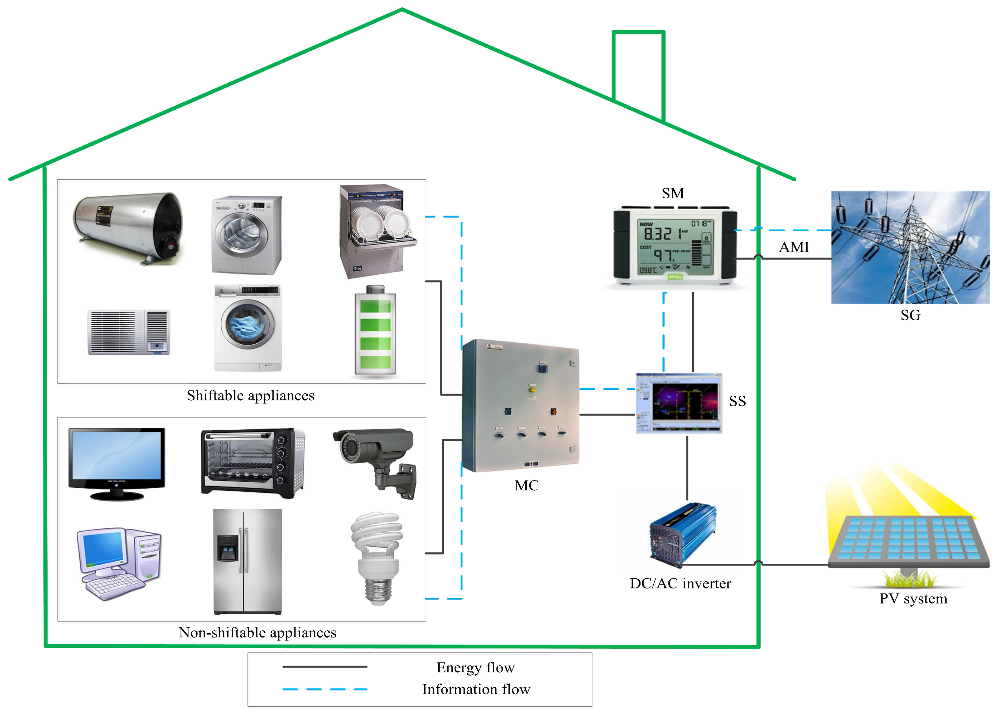
5. Proposed System Architecture

In SG, DSM and DR ensure more stable and reliable grid operation. The main objective behind the design and implementation of an HEMS is the reduction of electricity bill and PAR. From the utility point of view, its two main benefits are the management of energy resources and reduction of PAR. While from the consumers point of view, it minimizes the electricity bill. These objectives are achieved only with the modification in energy consumption pattern of shiftable appliances in response to DAP signal of electricity market defined and broadcasted by the utility.

In the proposed OHEMS, it is assumed that in future SG each prosumer will have a HEMS. To meet the energy demand with minimum electricity bill smart prosumer utilizes an in-house RES and an ESS along with grid energy. HEMS of the grid friendly prosumer schedules the appliances and the ESS to reduce the electricity bill and PAR in dynamic pricing environment of the electricity market. In this context, the prosumer’s appliances are divided into two categories: shiftable (i.e., their start time can be shifted to low price slots and would not be interrupted once they start operation) and non-shiftable (i.e., their start time can not be deferred and would not be interrupted during operation) appliances, as shown in

Table 4. Load categorization.

Shiftable Loads	Non-Shiftable Loads
Washing machine	Personal computers
Air conditioner	Security cameras
Clothes dryer	Microwave oven
Water heater	Refrigerator
Dish washer	Television
ESS	Lights

.

The proposed system architecture shown in Figure 1, mainly includes AMI, SM, smart scheduler (SS), master controller (MC), PV system, direct current (DC)/alternating current (AC) inverter, ESS, and appliances. In Figure 1 the energy flow is represented by solid lines while information flow is shown by dotted lines.

The integration of advanced ICTs into the conventional power grid for metering and communication is known as AMI. It works as a backbone of the SG and enables the two-way communication between the utility and the consumers. Furthermore, AMI is responsible for the collection and transmission of energy consumption data from SM to the utility as well as for the relaying of exogenous grid signals to the SM. The exogenous grid signals may be the price signal, ambient temperature, solar irradiance or DR signal. The SM works as a communication gateway between the SH and the utility. SM is typically installed between the AMI and EMC. The main functions of SM are reading, processing and sending of energy consumption data to the utility via AMI as well as the receiving and processing of DR and pricing signals from the utility. RSERs are considered as a real alternative to fossil fuel power generation. RSERs mainly includes PV system, wind turbines, small scale hydro-turbines and fuel cells. In the proposed scheme only PV system is utilized due to its easy installation and small capital investment. A DC/AC inverter is used to convert the PV system generated DC electricity into AC. An ESS works as a source and sink is regarded as a promising solution for the integration of RSERs into distribution networks/residential sector. Therefore, in the proposed OHEMS a small capacity ESS is used to efficiently exploit the PV system, and to reduce the electricity bill in peak hours. An SS installed between SM and MC is programmed using heuristic algorithms. The designed SS not only generates the optimal energy usage pattern for all appliances but also sends it to the MC for execution. MC is the core of proposed OHEMS and controls the operation of appliances and ESS according to the generated schedule by SS.

6. Scheduling Algorithms

The appliances scheduling problem formulated in Section 4 is solved by using GA, BPSO, WDO, BFO, and HGPO algorithms. Although, appliances scheduling problem has been solved by different classical optimization techniques: LP, ILP, MILP and DP. However, these techniques can not handle large number of appliances and face a lot of difficulties in convergence. Moreover, most of the classical algorithms do not have the global perspective and often converge at the local optimum solution. In contrast, the evolutionary algorithms: GA, BPSO, WDO, BFO, and HGPO algorithms give alternate methods to solve complex problems, and outperform the classical optimization techniques.

6.1. GA

GA is an iterative optimization algorithm inspired by the natural genetic process of the living organisms. Rather than working on a single solution, GA deals with different possible solutions in each iteration [41]. GA begins its search with randomly initialized binary coded chromosomes. The chromosomes pattern of GA represent the $ON/OFF$ state of appliances, and the length of chromosomes shows the number of appliances.

$$\mathit{Length}\mathit{of}\mathit{chromosomes}=\mathit{L}$$

(22)

where, L is the number of household appliances.

Once the population (a set of solutions that shows the status of each appliance in a particular time slot) is created, fitness function of each possible solution is evaluated according to the objective function of the optimization problem. Here, the fitness of each population is evaluated using Equation (18). Then, a new population is created by applying the natural genetic operators: crossover and mutation. The GA parameters with their values on which it gives optimal results are listed in

Table 5. Genetic algorithm (GA) parameters.

Parameters	Value
Number of iterations	500
Populationsize	200
$P_m$	0.1
$P_c$	0.9
n	11

.

The working flow of GA is shown in Figure 2. In each iteration, a new population is produced through crossover and mutation. In the crossover step, two binary strings are crossover to create a new off spring. Crossover probability says how often crossover will be performed. If there is no crossover, offspring is exact copy of parents. If there is a crossover, offspring is made from parts of parents’ chromosome. If crossover probability is 100%, then all offspring is made by crossover. If it is 0%, a whole new generation is made from exact copies of chromosomes from old population [42]. Moreover, a larger crossover rate avoids premature convergence to the sub-optimal solutions, so, the best crossover rate selected for optimization problems is 90% as given by,

$$P_c=0.9$$

(23)

To create randomness in the results so that the repetition of a population could be avoided we use mutation process. It changes one or more principles gene in a chromosome from its initial state. In natural genetic process, the probability of mutation is very low, so, an optimum mutation rate for optimization problems is,

$$P_m=1-P_c$$

(24)

Once crossover and mutation are done, again a population is generated and fitness is evaluated and compared with previous population.

6.2. BPSO

PSO is a nature-inspired optimization algorithm for finding an optimal solution within the search space. The PSO algorithm inherently exists in the continuous domain. However, it can be modified into the discrete domain, and its variants for the discrete domain is BPSO. The working flow of BPSO shown in Figure 3, mainly depends on four factors; initial position, initial velocity, particle own best position and global best position among all the particles. In this algorithm, a population is randomly initialized and scattered in the search space. The initial positions and velocities of the particles are represented by $x_i$ = $x_1+x_2+\cdots +x_I$ and $V_i$ = $V_1+V_2+\cdots +V_I$ respectively. The particles update their velocities in each iteration by using Equation (25) [43],

$$\begin{array}{c}\hfill \sum _{t=1}^{24}\sum _{i=1}^I{V}_i^{t+1}=\sum _{t=1}^{24}\sum _{i=1}^I(w{V}_j^t\left(j\right)+c_1{r}_1\left(X_{lbest,i}\left(j\right)\right)-x_i^t\left(j\right))+c_2{r}_2(X_{gbest,i}\left(j\right)-x_i^t\left(j\right))\end{array}$$

(25)

where $V_i^{t+1}$ is the velocity of particle (appliance) in upcoming time slot, w is inertia factor, $V_j^t$ is current velocity, $r_1$ and $r_2$ are random numbers, $c_1$ and $c_2$ are local and global pulls respectively, $x_i^t$ is the particle current position, $X_{lbest}$ is local best position and $X_{gbest}$ global best position. The velocities of the particles are mapped between 0 and 1 by using sigmoid function given by Equation (26),

$$sig\left(V_i^{t+1}\left(j\right)\right)=\frac{1}{1+exp(-V_i^{t+1}\left(j\right))}$$

(26)

The random values assigned to each particle in the population are compared with the sigmoid function to generate a binary coded population.

$$x_i^{t+1}=\left\{\begin{array}{cc}1\hfill & sig\left(V_i^{t+1}\left(j\right)\right)<r_{ij},\hfill \\ 0\hfill & otherwise.\hfill \end{array}\right.$$

(27)

In each iteration, particles record their positions with respect to neighbors. The local best positions found by the particles are represented as $X_{lbest}$ = $X_{lbest1}+X_{lbest2}+\cdots +X_{lbestN}$. The local best values are then compared with each other to find the global best position. The $g^{th}$ particle among the particles is said to be the global best position if it satisfy the objective function, and the global best positions are represented as $X_{gbest}$ = $X_{gbest1}+X_{gbest2}+\cdots +X_{gbestN}$. The main reason behind the use of global best value rather than local best value is its faster convergence to the optimal solution. The global best value is a binary coded string and represents the optimal $ON/OFF$ status of the appliances. The fitness function of each particle is evaluated and compared with the corresponding cost of global best value, and the string with minimum fitness function is selected. The BPSO parameters and their values on which BPSO gives optimal results are given in

Table 6. Binary particle swarm optimization (BPSO) Parameters.

Parameters	Values
Number of iterations	300
Swarmsize	200
$v_{max}$	4
$v_{min}$	−4
$w_i$	2
$w_f$	0.4
$c_1$	2
$c_2$	2
n	11

.

6.3. WDO

WDO is an another nature-inspired optimization algorithm based on the atmospheric motion of air parcels. In this algorithm, infinitely small air parcels move in N-dimensional search space. The major difference between the WDO and other heuristic algorithms is the use of four different forces to control the motion of air parcels in the atmosphere. These forces include pressure gradient force, friction force, gravitational force, and Coriolis force. The pressure gradient force moves the air parcels in the forward direction, while the frictional force resists their motion in the forward direction. Furthermore, the gravitational force is a vertical force in three-dimensional search space that attracts the air parcels towards the origin, and the deflection of air parcels in the atmosphere is due to the Coriolis force. Mathematically, all four forces are represented as [44].

$$F_{pg}=-\Delta \rho \delta \nu$$

(28)

$$F_C=-2\mathsf{\Omega }\times \mu$$

(29)

$$F_G=\rho \delta \nu \times g$$

(30)

$$F_F=-\rho \alpha \mu$$

(31)

where $F_{pg}$ is pressure gradient force, $\Delta$ is pressure gradient, $\rho$ is air density, $\delta \nu$ is finite volume of the air, $F_C$ is Coriolis force, $\mathsf{\Omega }$ represents the rotation of the earth, $\mu$ is velocity vector of the wind, $F_G$ vertical force directed toward the earth’s surface, g is acceleration of gravity, $F_F$ is friction force, and $\alpha$ is friction coefficient.

In each iteration, the position and velocity of the air parcels are updated by [44],

$$\begin{array}{c}\hfill {\nu }_{new}=((1-\alpha ){\nu }_{old}-g{x}_{old}+\left[\right|\frac{P_{max}}{P_{old}}\left|RT(x_{max}-x_{old})\right]-\frac{c{\nu }_{old}}{P_{old}}\end{array}$$

(32)

and

$$x_{new}=x_{old}+({\nu }_{new}\times \Delta t)$$

(33)

In Equation (32), the $\left((1-\alpha ){\nu }_{old}\right)$ represents the opposite force continuously pushing the air parcels towards their previous positions. Whereas the $g{x}_{old}$ shows the gravitational force which attracts the air parcels towards the center of the earth. The motion of the air parcels towards the high-pressure point/global best position is described by $\left[\right|\frac{P_{max}}{P_{old}}\left|RT(x_{max}-x_{old})\right]$ and $\frac{c{\nu }_{old}}{P_{old}}$ explains the Coriolis force which controls the motion of the air parcels.

WDO creates random solutions from the n number of air parcels. After evaluating the fitness function, and updating velocities a new population is generated. The fitness function of the new and old air parcels are compared to obtain an optimal appliance scheduling pattern. The pressure term used in WDO is just like fitness term used in GA, BPSO and HGPO. The WDO parameters and their values that give optimal results are given in

Table 7. Wind driven optimization (WDO) parameters.

Parameters	Values
Number of iterations	500
Populationsize	200
dimMin	$-5$
dimMax	5
$v_{min}$	$-0.3$
$v_{max}$	0.3
RT	3
n	11
g	0.2
$\alpha$	0.4

and the main steps involved in WDO algorithm are shown in Figure 4.

6.4. BFO

BFO is a new addition to the family of nature-inspired optimization algorithms. BFO algorithm is inspired by the social foraging behaviour of Escherichia coli. Since its inception, BFO has drawn the attention of researchers from diverse fields of knowledge. In the BFO algorithm, the bacteria swim in search of nutrients and select the best nutrients (solutions) to maximize its energy. The parameters used in BFO and the values on which it gives optimal results are listed in

Table 8. BFO parameters.

Parameter	Value
Maximungeneration	500
$N_e$	24
$N_r$	5
$N_c$	5
$N_p$	30
$N_s$	2
$C_i$	0.01
$P_{ed}$	0.5
$\theta$	0.5

.

BFO algorithm consists of four steps; Chemotaxis, Swimming, Reproduction, and Elimination-dispersal. BFO algorithm starts its search with parameters initialization, and after initialization of parameters, under the chemotaxis step, initial states of appliances are evaluated and then our system computes the new positions of bacteria (solution matrix). Mathematically the chemotaxis steps of a bacterium can be represented by Equation (34) [45],

$$\begin{array}{c}\hfill {\theta }^i(j+1,k,l)={\theta }^i(j,k,l)+C\left(i\right)\frac{\Delta \left(i\right)}{\sqrt{{\Delta }^T\left(i\right)\Delta \left(i\right)}}\end{array}$$

(34)

where ${\theta }^i$ ($j,k,l$) represents i-th bacterium at j-th chemotactic, k-th reproductive and l-th elimination-dispersal step. $C\left(i\right)$ is the size of step taken in the random direction specified by the tumble, and $\Delta$ indicates a vector in the random direction whose elements lie in [$-1$, 1].

In next step, swimming loop is initialized to find the current best state of appliances. The swimming step is represented by Equation (35) [46],

$$\begin{array}{c}\hfill J_{cc}(\theta ,P(j,k,l))=\sum _{i=1}^S{J}_{cc}({\theta }^i,\theta (j,k,l))=\sum _{i=1}^S[-d_{attractant}exp(-w_{attractant}\sum _{m=1}^n{({\theta }_m-{\theta }_m^i)}^2)]\\ \hfill +\sum _{i=1}^S[-h_{repellant}exp(-w_{repellant}\sum _{m=1}^n{({\theta }_m-{\theta }_m^i)}^2)]\end{array}$$

(35)

where $J_{cc}$ ($\theta$, P( j, k, l)) is the objective function, S is the total number of bacteria, n is the number of appliances, and $\theta$=[${\theta }_1$,${\theta }_1$,⋯,${\theta }_n$]${}^n$ is a n-dimensional search space. The $d_{attractant}$, $w_{attractant}$, $h_{repellant}$ and $w_{repellant}$ are different coefficients that should be selected properly [47].

When swimming steps complete, iterations of reproduction loop start in which only feasible solutions are recorded to produce next generation. Then, the elimination-dispersion steps discard the least feasible solutions, and new random samples are inserted with a low probability. This is a very important process because infeasible solutions are eliminated, and the chances of repetition are avoided. The working flow of BFO algorithm is shown in Figure 5.

6.5. HGPO

Our proposed HGPO algorithm combines the features of BPSO and GA to effectively reduce the electricity bill and PAR. The GA and BPSO are chosen for hybridization because the GA is good in PAR reduction, and BPSO is effective in bill reduction. Working procedure of HGPO consists of two stages, first, all steps of BPSO are followed, then, the crossover and mutation operators of GA are applied to the current global best position $X_{gbest}^t$ and the previous global best position $X_{gbest}^{t-1}$ found by BPSO algorithm. The application of crossover and mutation operators to the best positions give better results than their application to the random population. The proposed HGPO algorithm is shown in Figure 6.

7. Results and Discussions

In this section, simulation results of the proposed OHEMS are presented. In the proposed scheme, the integration of RES and ESS, as well as the performance of various heuristic algorithms (GA, BPSO, WDO, BFO, and HGPO), is evaluated via two stages simulations. In the first case, the integration of RES and ESS into the residential sector are evaluated in terms of energy consumption pattern, and electricity bill as well as PAR reduction. While in the second case, the same performance metrics (energy consumption pattern, and electricity bill as well as PAR minimization) are used to evaluate the effectiveness of GA, BPSO, WDO, BFO and HGPO algorithms for HEMSs. For simulations, we have used MATLAB installed on Intel(R) Core(TM) i3-2370M CPU @ 2.4GHz and 2GB RAM with Windows 7. The computational time of all heuristic algorithms is given in

Table 9. Computational time.

Algorithm	Computational Time (Sec)
GA	2.21
BPSO	1.86
WDO	2.84
BFO	3.59
HGPO	1.71

.

To demonstrate the proposed OHEMS, an end user with 11 passive appliances and an ESS which works as a source and sink is considered. The descriptions of the appliances are shown in

Table 10. Description of the appliances.

Load Type	Appliances	Power Rating (kW)	Daily Usage (Hours)
Shiftable	ESS	3	–
	Washing machine	0.8	5
	Air conditioner	1.3	10
	Clothes dryer	0.7	4
	Water heater	1	8
	Dish washer	0.2	3
Un-shiftable	Personal computers	0.2	18
	Security cameras	0.1	24
	Microwave oven	0.5	7
	Refrigerator	0.9	20
	Television	0.2	8
	Lights	0.1	6

, the column III shows the power rating of the appliances and column IV shows the length of operation time of the corresponding appliance. In this paper, the length of operation time is arbitrarily taken and remains the same in both scenarios (i.e., unscheduled and scheduled) to have a fair comparison. It is assumed that the utility power supply is available around the clock to support the prosumer’s load. Moreover, the utility has AMI to get the forecasted data of weather conditions, ambient temperature, and solar irradiance from the metrological department, and to broadcast it to the prosumers. The exogenous grid signals (DAP signal, forecasted ambient temperature, and solar irradiance) used in the proposed OHEMS are shown in Figure 7, Figure 8 and Figure 9 respectively. The DAP shown in Figure 7 is defined by the utility operator and the normalized form of solar irradiance and temperature data obtain from METEONORM 6.1 for Islamabad region of Pakistan is presented in Figure 8 and Figure 9.

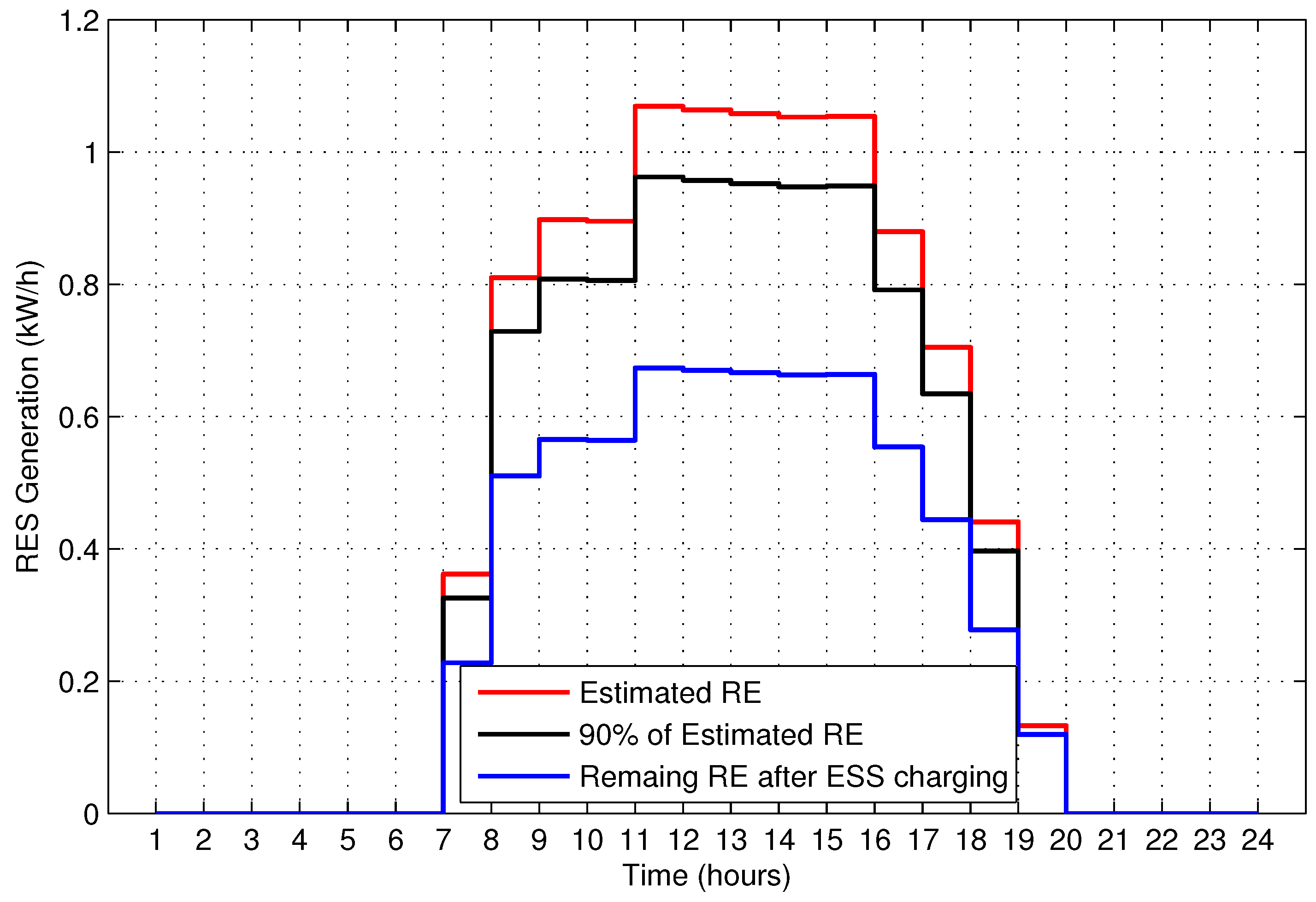
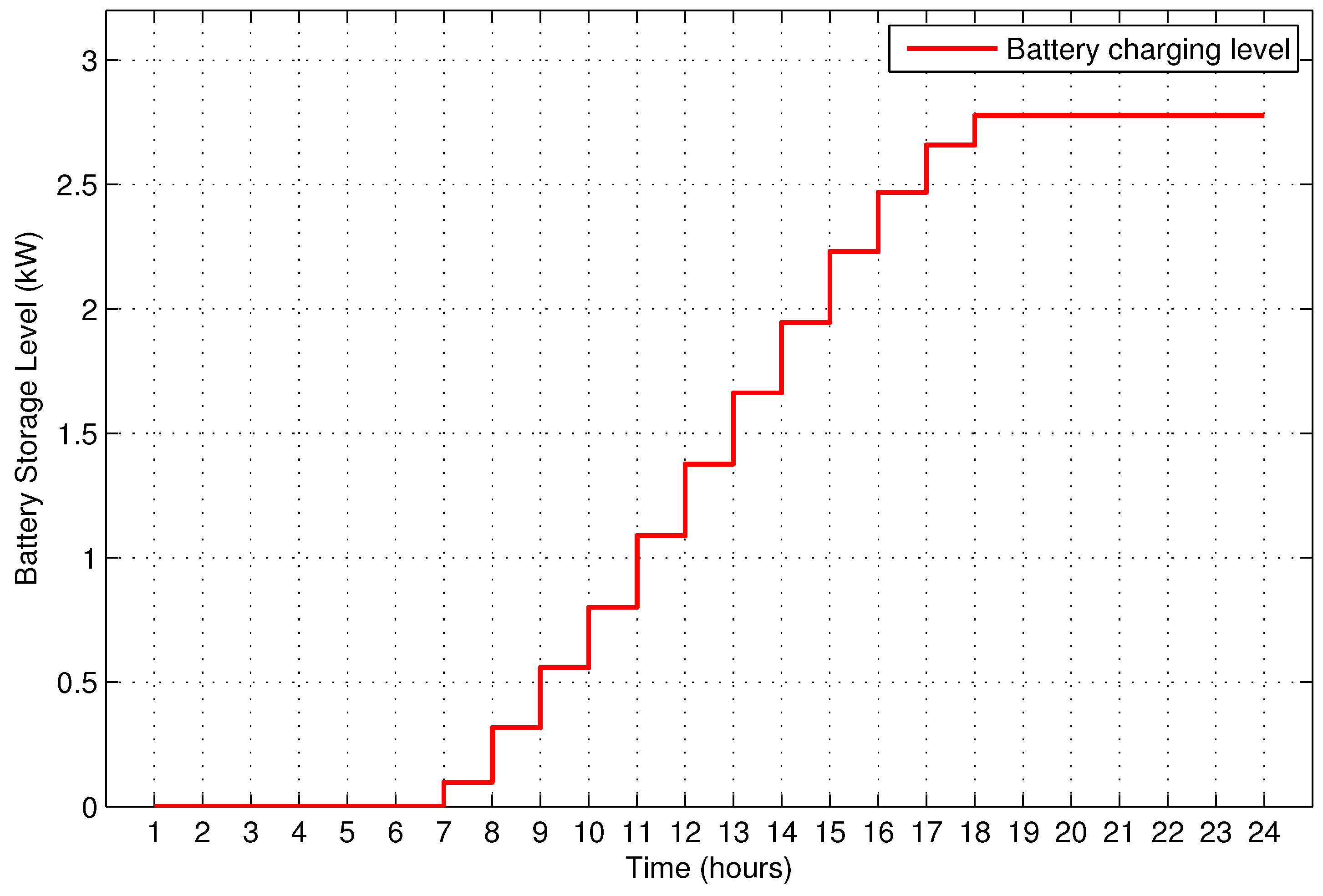
The electricity generation by PV system modeled in Equation (1) mainly depends on energy conversion efficiency of the solar generator, the effective area of the generator, solar irradiance, and ambient temperature. Ninety percent of the estimated RE in any time slot of the scheduling horizon is considered for consumption. This uncertainty of 10% is included to cater for the disparity between the estimated and the actual generation. Moreover, 30% of the 90% of estimated RE in each time slot is used for the charging of ESS as long as the charging level of ESS is between 10–90%. The estimated RE, RE after taking 10% uncertainty, remaining RE after the charging of ESS and charging level of ESS system are presented in Figure 10 and Figure 11 respectively. The ESS is charged only from the PV system in the day time. After the ESS charged fully, it is utilized in a high price time slot i.e., $\tau$ as given by Equation (17).

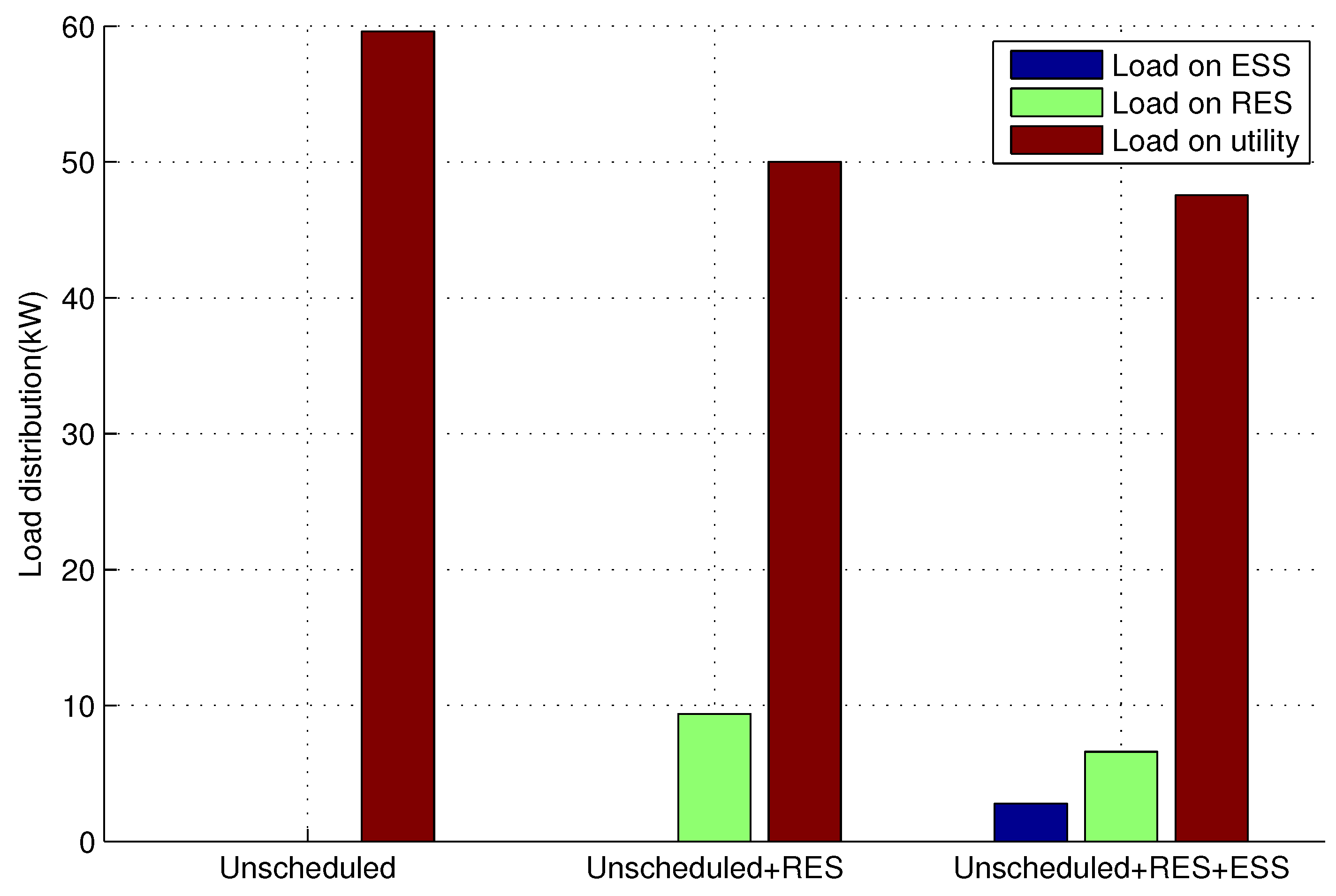
7.1. Case 1: Integration of RES and ESS

In this case, the benefits of RES and ESS integration into the residential sector are highlighted in terms of energy consumption pattern, and electricity bill as well as PAR reduction. The load distribution among the utility, RES and ESS is shown in Figure 12. It illustrates that in second scenario a portion of the prosumer load shifted from utility to RES, and in the third scenario an ESS is also integrated to support the prosumer’s load in peak hours.

7.1.1. Energy Consumption

To explain the behavior of the energy consumption pattern, we define some arbitrary thresholds. The descriptions of load and thresholds are given in

Table 11. Thresholds of energy consumption.

Load	Range (kW)
High peak	5 and above
Peak	4–4.9
Moderate	2–3.9
Minimum	1–1.9
Negligible	0.1–0.9

.

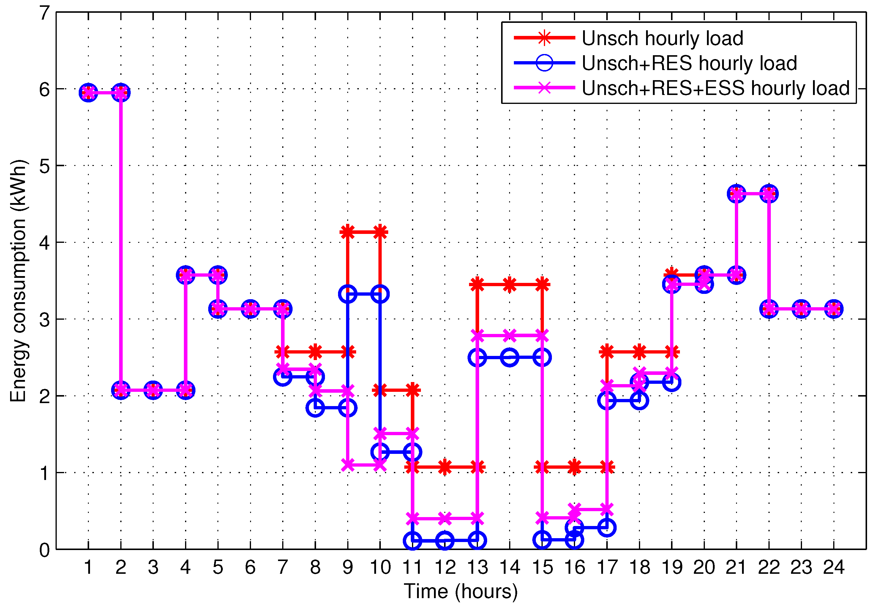
The energy consumption pattern of the prosumer load is shown in Figure 13. Results illustrate that in the first scenario (unscheduled load without RES and ESS), the energy consumption pattern has a high peak load of 5.95 kW in time slot 1, and peak loads of 4.7 kW and 4.2 kW in time slots 21 and 9 respectively. Moreover, the energy consumption pattern shows a moderate behaviour in time slots 2–8, 10, 13–14, 17–20 and 22–24, and minimum energy is consumed in time slots 11–12 and 15–16.

The energy consumption pattern of the second scenario (unscheduled load with RES), shows that the energy consumption remains the same in time slots 1–6 and 20–24. This is because the RE is available from the PV system as shown in Figure 10. This illustrates that the in-house RES generates electricity only in the time slots 7–19. Therefore, in time slots 7–19, the energy consumption is reduced by the corresponding amount of RE available in that time slot.

In the third scenario (unscheduled load with RES and ESS), we also integrate an ESS to the proposed SH. After the integration of ESS, energy consumption remains same in time slots 1–6 and 20–24; however, in time slots 7–8 and 10–19 the energy consumption becomes higher than the second scenario. This increase occurs because 30% of the RE available in time slots 7–19 is used for the charging of ESS. While, in time slot 9, the ESS is discharged and load on the utility is reduced by 73.60% and 67.16% as compared to first and second scenarios respectively.

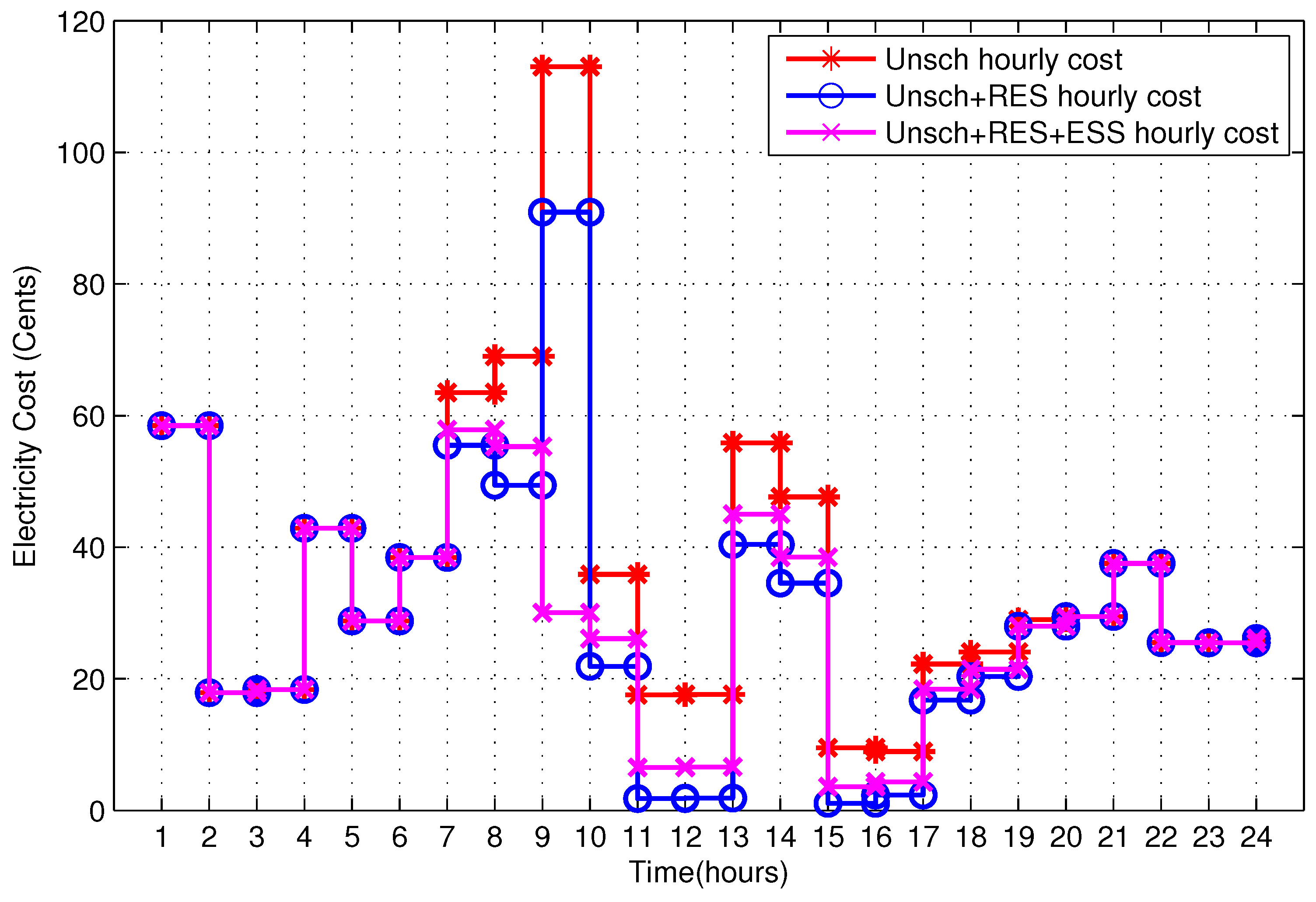
7.1.2. Electricity Cost

The corresponding electricity bill of the energy consumption is shown in Figure 14. Results illustrate that in time slots 1–6 and 20–24 the electricity bill of all the three scenarios remains the same. While, in time slots 7–19, the RE is available and significantly reduces the electricity bill. Particularly, in time slot 9, the RE reduces the electricity bill by 19.55%, and after the discharge of ESS, the total reduction of 71.41% is achieved in the electricity bill.

7.1.3. Total Cost

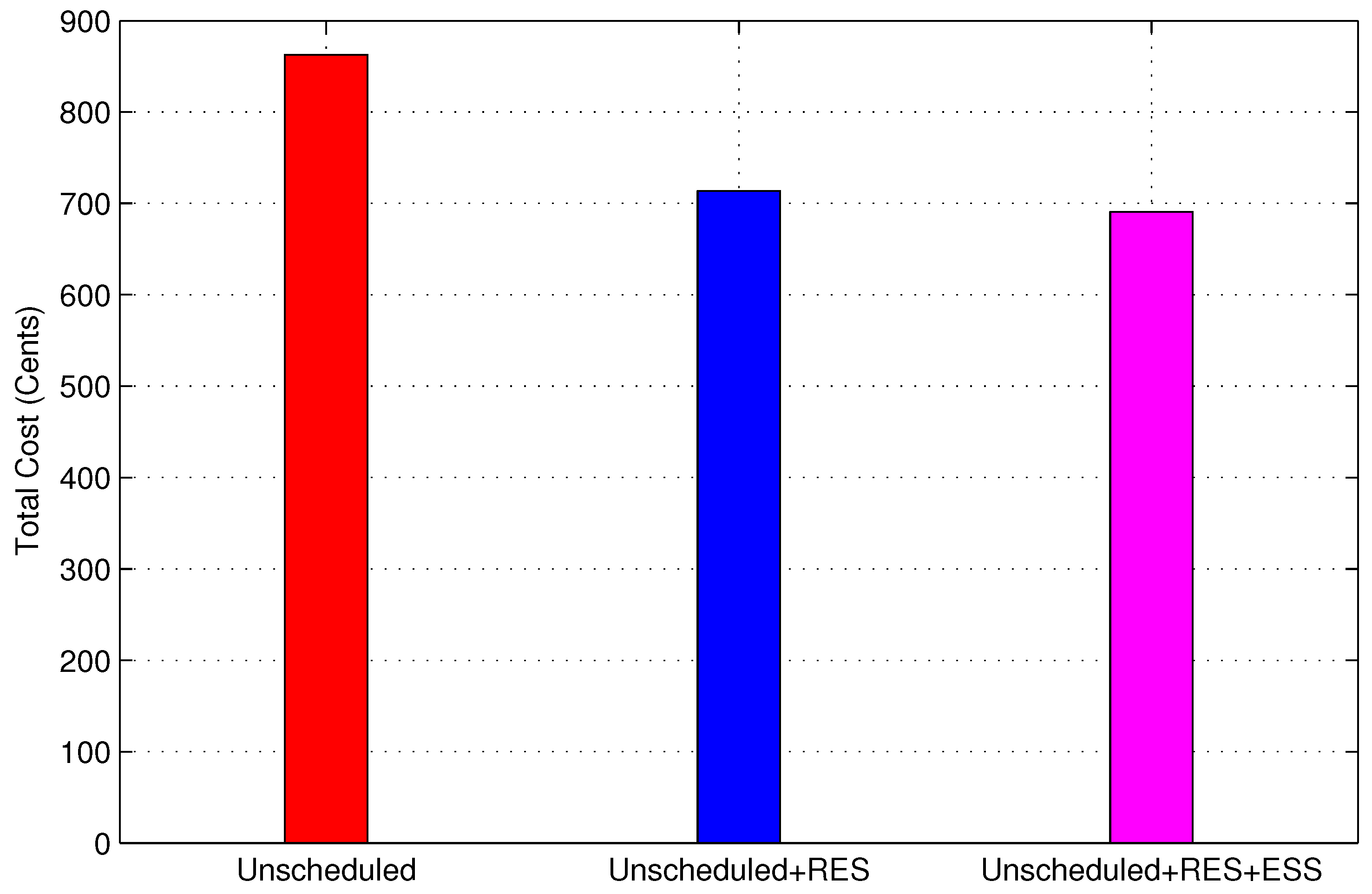
The total electricity bill of case 1 is shown in Figure 15. Results illustrate that the investment of a small capital cost on the integration of RES reduces the electricity bill by 17.25%, and after adding EES too, the bill is reduced by 19.94%. The reduction in electricity bill due to RES and ESS is summarized in

Table 12. Comparison of case 1 cost.

Scenario	Cost (Cents)	Difference (Cents)	Reduction (%)
Unscheduled	862.66	-	-
Unscheduled + RES	713.78	148.88	17.25%
Unscheduled + RES + ESS	690.63	172.03	19.94%

.

7.1.4. PAR

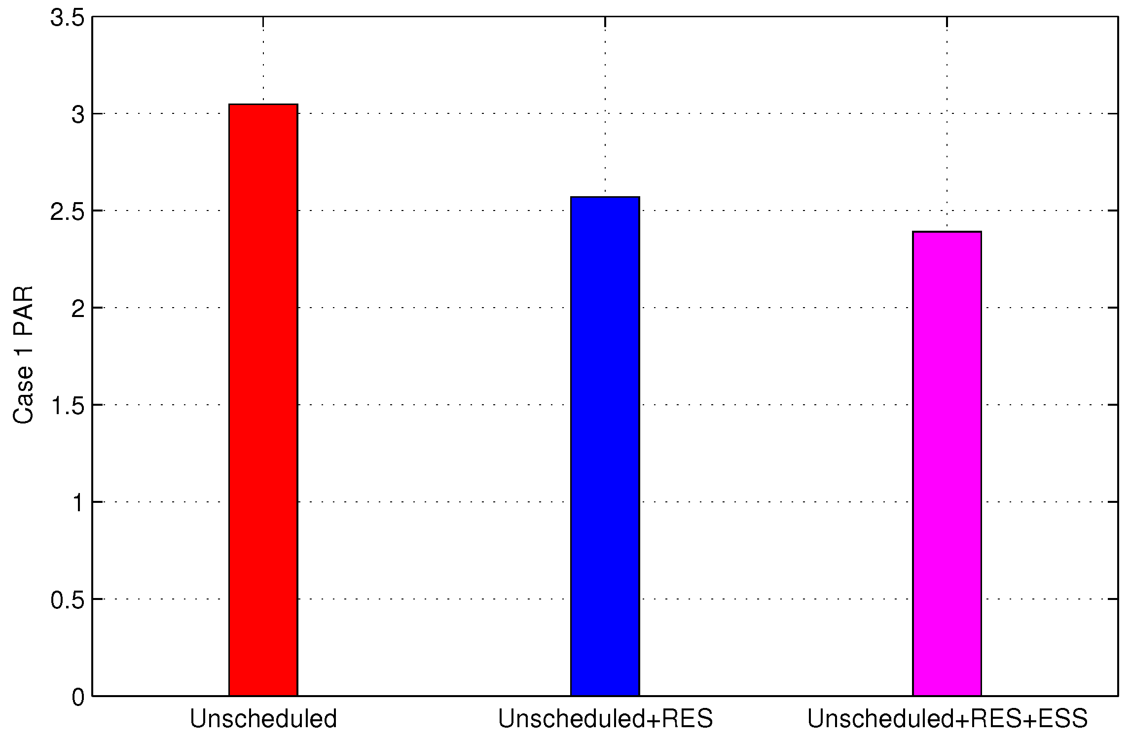
The PAR of the prosumer load is shown in Figure 16. Results illustrate that the integration of RES reduces the PAR by 15.68% and after incorporating the ESS as well, the PAR is reduced by 21.55%. The reduction in PAR in all three scenarios is shown in

Table 13. Comparison of case 1 PAR.

Scenario	PAR	Difference	Reduction (%)
Unscheduled	3.0482	-	-
Unscheduled + RES	2.5702	0.478	15.68%
Unscheduled + RES + ESS	2.3912	0.657	21.55%

. This reduction in PAR not only enhances the stability and reliability of the power system but also reduces the electricity bill of the prosumer.

7.2. Feasible Region of the Objective Function

The feasible region of the objective function (electricity bill) formulated in Equation (18) is shown in Figure 17. In Figure 17, the trapezoid of $P_1(0.1,0.81)$, $P_2(0.1,2.735)$, $P_4(6,48.6)$ and $P_6(6,164.2)$ represents the overall region of electricity bill. Where, the point $P_1(0.1,0.81)$ represents the electricity bill when minimum possible load (0.1 kW) is scheduled in minimum price slot (21) of RTP signal, and if the energy consumption is 0.1 kW in the maximum price slot (9) of RTP signal, the electricity bill will be represented by the point $P_2(0.1,2.735)$. Moreover, the points $P_4(6,164.2)$ and $P_6(6,48.6)$ represent the bill when all appliances are in ON status in minimum and maximum price slots of RTP signal respectively. Equation (18) shows that the objective function depends on two factors: amount of load and electricity price in that time slot. The price signal is defined by the utility and we have no control over it; therefore, to minimize the electricity bill we can only modify the shape of the energy consumption pattern. Furthermore, in scheduled load scenarios, the electricity cost in any time slot must not exceed the maximum cost of the unscheduled scenario, i.e., 59.5 cents. After applying the limit of 59.5 cents the feasible region of scheduled load electricity bill is shown by the pentagon of $P_1(0.1,0.81)$, $P_2(0.1,2.735)$, $P_3(2.13,59.5)$, $P_5(6,59.5)$ and $P_6(6,48.6)$. Where, the point $P_3(2.13,59.5)$ shows that in maximum price time slot of RTP signal the scheduled load must not exceed than 2.13 kW, and point $P_5(6,59.5)$ shows that the maximum possible load (6 kW) must not be scheduled in time slots having price greater than 9.92 cents.

7.3. Case 2: OHEMS with Integrated RES and ESS

The distribution of the prosumer load among the utility, RES and ESS is illustrated in Figure 12. It shows that in the second scenario of case 1, an RES is integrated to the SH while, in the third scenario, an ESS is also utilized to support the prosumer’s load.

Here, in this section, the simulation results of the heuristic algorithms (GA, BPSO, WDO, BFO and HGPO) based OHEMS are presented. In this case, the cost of unscheduled load with RES and ESS is taken as a reference to validate the effectiveness of the heuristic algorithms for HEMSs. The performance of heuristic algorithms (GA, BPSO, WDO, BFO and HGPO) is evaluated by using the same performance metrics (energy usage pattern, and electricity bill as well as PAR reduction) of case 1. The designed SS generates an optimal energy usage pattern for shiftable appliances in response to grid signals and a large portion of load is shifted toward off-peak hours. This relocating of load significantly reduces the electricity bill as well as the PAR. Simulation results of the proposed scheme are as follows:

7.3.1. Energy Consumption

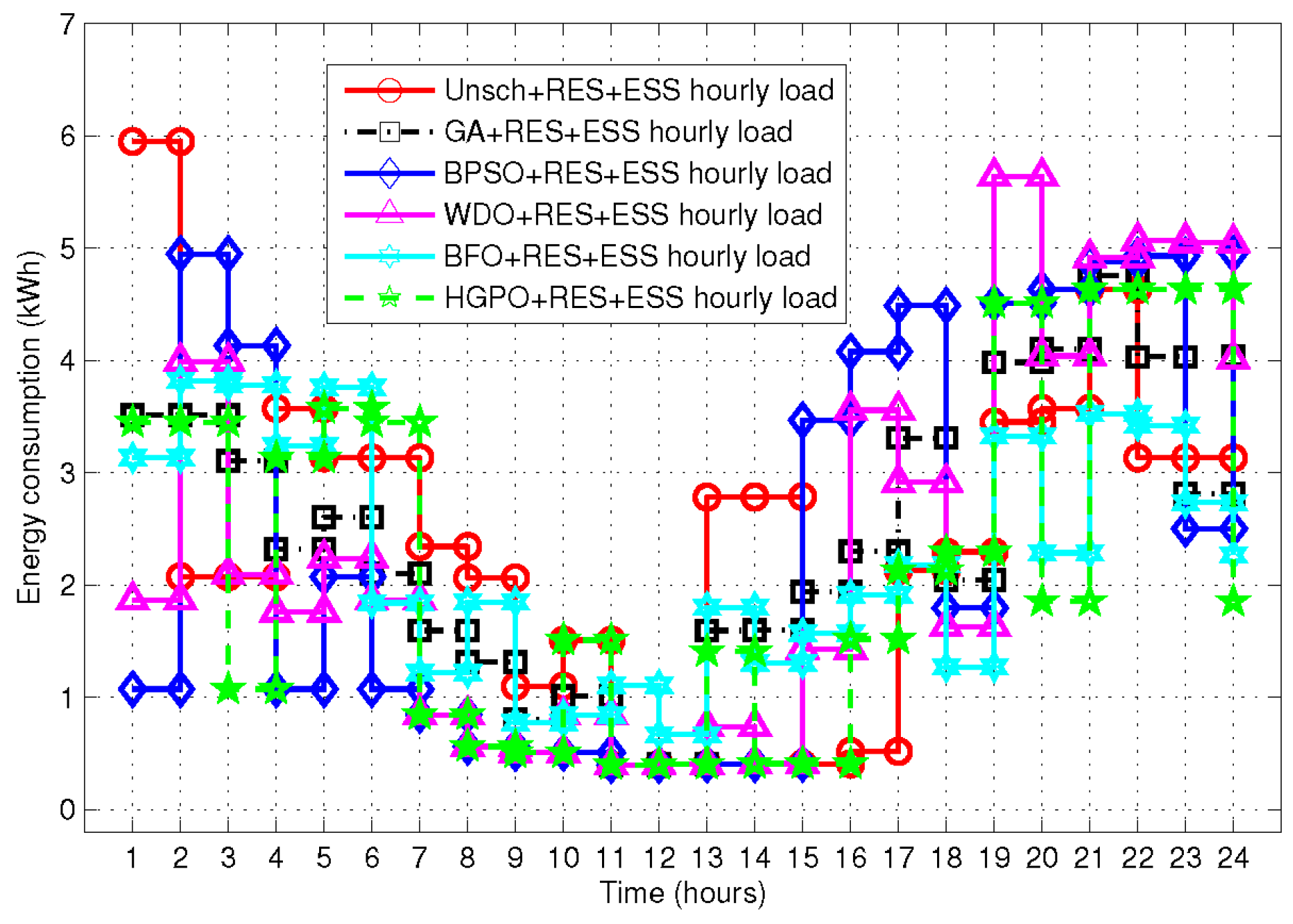
The energy consumption patterns of scheduled and unscheduled loads with RES and ESS are shown in Figure 18. In unscheduled load with RES and ESS scenario, the prosumer’s energy consumption pattern has a high peak of 5.95 kW in time slot 1 and followed by a peak load of 4.8 kW in time slot 21. A moderate behaviour of load is recorded in time slots 2–8, 13–14, 17–20, and 22–24. Moreover, the energy consumption is found to be minimum in time slots 9–10, and negligible in time slots 11–12 and 15–16.

GA-based scheduling creates no high peaks, and a peak load of 4.75 kW is consumed in time slot 21; 4.12 kW in time slot 20; 4.07 kW in time slot 22; and 4.01 kW in time slot 24. The energy consumption pattern is found to be moderate in time slots 1–6, 16–19 and 23. Furthermore, the energy consumption is minimum in time slots 7–8, 10 and 13–15, and negligible in time slots 9 and 11–12. The comparison of GA-based scheduled and unscheduled load shows that the maximum load in GA-based scheduling is 20.16% less than the maximum load in the unscheduled scenario.

BPSO-based scheduling also does not create high peaks, and the energy consumption pattern has peak load of 4.96 kW in time slots 2 and 22; 4.9 kW in time slot 21; 4.81 kW in time slot 20; 4.76 kW in time slot 19; 4.67 kW in time slots 17 and 19; 4.2 kW in time slot 3; and 4.12 kW in time slot 16. The energy consumption is found to be moderate in time slots 5, 15 and 23. Additionally, a minimum amount of energy is consumed in time slots 1, 4, 6 and 18, and negligible in time slots 7–14. The comparison of BPSO-based scheduled and unscheduled load shows that the maximum load in BPSO is 16.63% less than the maximum load in the unscheduled scenario.

In WDO-based scheduling, a high peak load of 5.75 kW is consumed in time slot 19 and 5.12 kW in time slots 22–23. The energy consumption pattern has peak load of 4.95 kW in time slot 21; 4.08 kW in time 20; and 4 kW in time slots 2 and 24. In addition, a moderate amount of energy is consumed in time slots 3, 5, 16 and 17. The energy consumption is minimum in time slots 1, 4, 6, 15 and 18, and negligible in time slots 7–14. The comparison of WDO-based scheduled and unscheduled load shows that the maximum load in WDO is 3.36% less than the maximum in the unscheduled scenario.

The BFO algorithm neither creates high peaks nor peaks in energy consumption pattern. The energy consumption is moderate in time slots 1–5, 17 and 19–24, and minimum in time slots 6–8, 11, 13–16 and 18. Moreover, the energy consumption is negligible in time slots 9–10 and 12. The comparison of BFO-based scheduled and unscheduled load shows that the maximum load in BFO is 36.13% less than the maximum load in the unscheduled scenario.

The proposed HGPO-based scheduling creates no high peaks, and a peak load of 4.7 kW is consumed in time slot 19 and 4.61 kW in time slots 21–23. The energy consumption is moderate in time slots 1–2, 4–6, 17 and 18. Moreover, minimum load is scheduled in time slots 3, 10, 13, 16, 20 and 24, and negligible in time slots 7–9, 11–12 and 14–15. The comparison of HGPO-based scheduled and unscheduled load shows that the maximum load in case of HGPO is 22.52% less than the maximum load in the unscheduled scenario.

Figure 18 illustrates that the load shifting pattern of HGPO is balanced, and uniformly distribute the load over the scheduling horizon. On the other hand, the other heuristic algorithms either completely shift the load towards off-peak hours or consume higher energy in peak hours. The HGPO outperforms the GA, BPSO, WDO and BFO algorithms by allowing the appliances to complete their tasks with minimum delay and avoids peak formation as well.

7.3.2. Electricity Cost

The corresponding electricity bill of unscheduled and scheduled load with RES and ESS is shown in Figure 19. Results illustrate that the electricity bill of heuristic algorithms (GA, BPSO, WDO, BFO and HGPO) based scheduled load remains within the feasible region. In GA-based scheduling, the maximum electricity bill is 39.7 cents in time slot 7. The electricity bill in case of BPSO has a maximum value of 43.6 cents in time slot 2 which is also less than the maximum bill (59.5) of unscheduled scenario. In the case of WDO, the maximum electricity bill is 47.3 cents in time slot 21, and the bill in all other slots also remains within the feasible region. The BFO-based scheduled load has maximum bill of 49.8 cents in a time slot 8. In the proposed HGPO algorithm, the electricity bill satisfies all the limits of the feasible region, and a maximum bill of 43.6 cents is recorded in time slot 6. Moreover, in peak hours the electricity bill of scheduled load is comparatively less than the unscheduled load, and the comparison of total electricity bills of the heuristic algorithms shows that the performance of HGPO-based HEMS in term of bill reduction is better than GA, BPSO, WDO and BFO based HEMS.

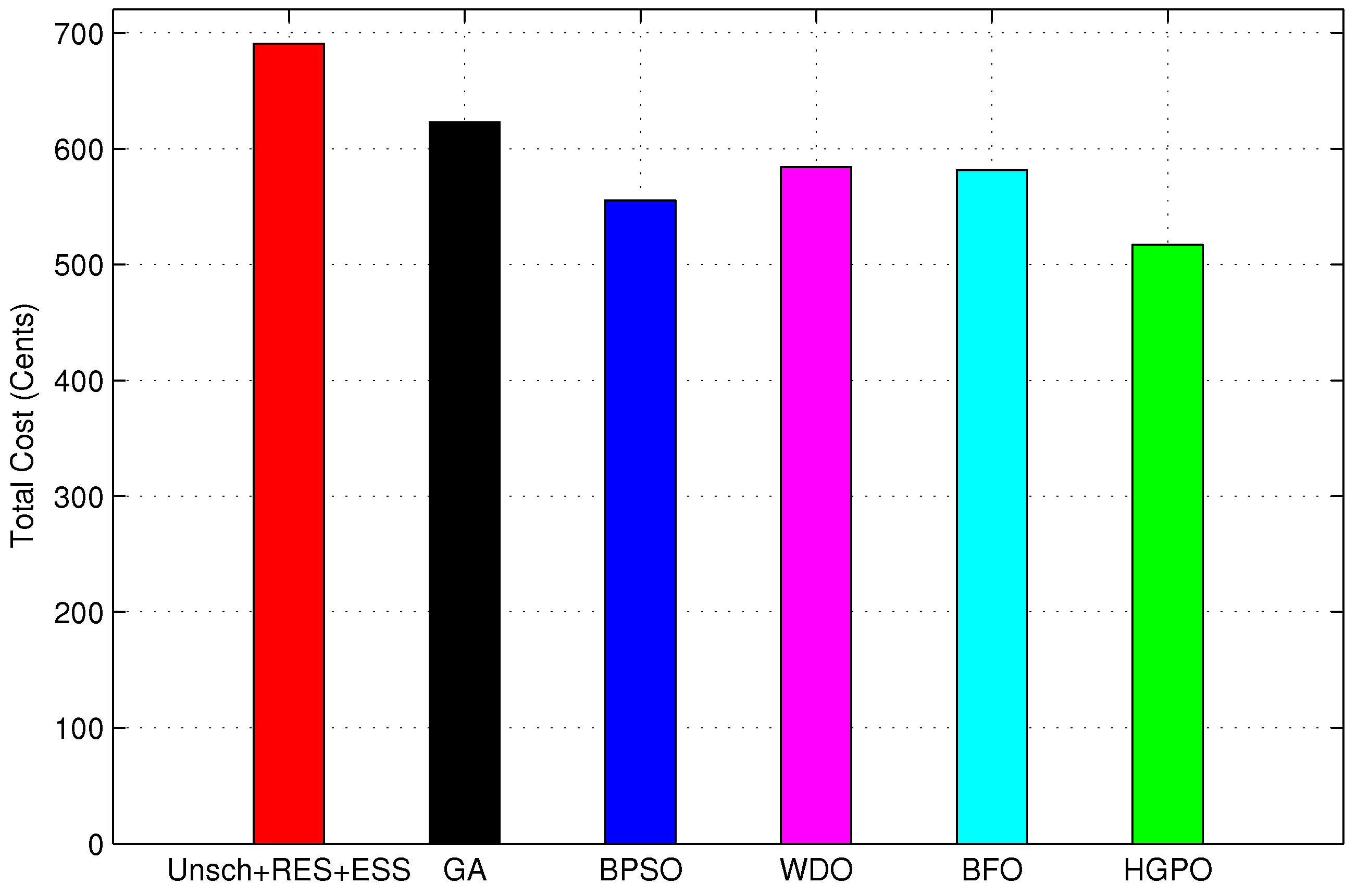
7.3.3. Total Cost

The comparison of overall electricity bill of the unscheduled and scheduled load with RES and ESS is shown in Figure 20. The total electricity bill in unscheduled, and in scheduled load scenarios using GA, BPSO, WDO, BFO and HGPO algorithms are 690.63, 622.97, 555.32, 584.24, 581.56 and 517.15 cents respectively. The comparison of total electricity bill shows that GA, BPSO, WDO, BFO and HGPO algorithms based HEMS reduces the electricity bill by 9.80%, 19.60%, 15.40%, 15.80%, and 25.12% respectively. The changes in electricity bill due to scheduling are listed in

Table 14. Comparison of case 2 cost.

Scheduling Technique	Cost (Cents)	Difference (Cents)	Reduction (%)
Unscheduled + RES + ESS	690.63	-	-
GA scheduled + RES + ESS	622.97	67.66	9.80%
BPSO scheduled + RES + ESS	555.32	135.31	19.60%
WDO scheduled + RES + ESS	584.24	106.39	15.40%
BFO scheduled + RES + ESS	581.56	109.07	15.80%
HGPO scheduled + RES + ESS	517.15	173.48	25.12%

. In peak hours the electricity charges of heuristic algorithms based scheduled load scenarios are significantly less than the unscheduled scenario. However, when the overall cost reduction is concerned the HGPO gives better results than the other optimization algorithms. Moreover, the electricity consumption pattern of HGPO is uniform, while the GA, BPSO, WDO and BFO algorithms create new peaks in off-peak hours that degrade their overall performance.

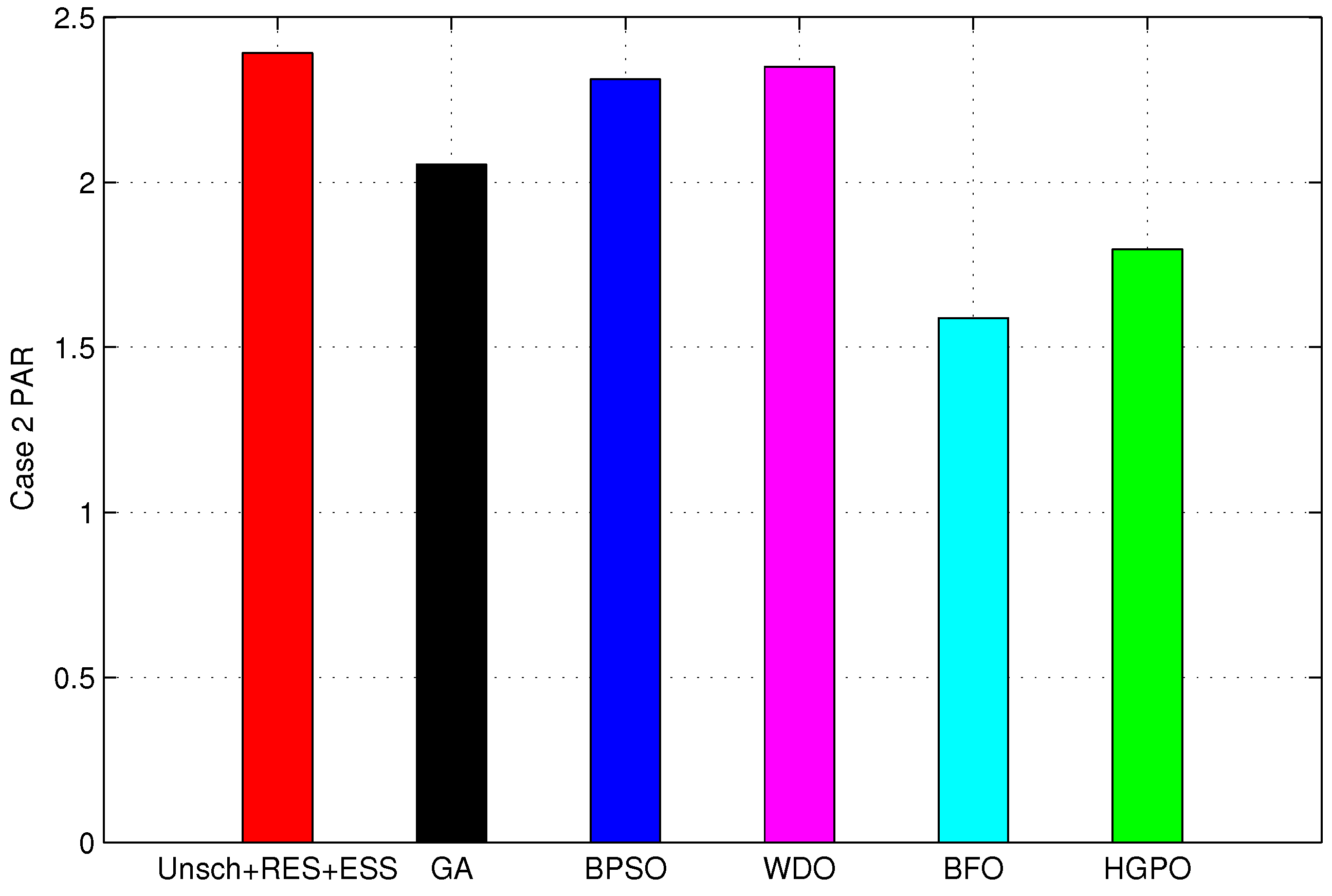
7.3.4. PAR

The PAR of unscheduled and scheduled load is shown in Figure 21. It illustrates that the proposed HGPO algorithm minimizes the PAR by 24.88%. The GA, BPSO, WDO and BFO algorithms also reduce the PAR by 14.09%, 3.30%, 22.10% and 33.54% respectively. The changes in PAR of the heuristic algorithms based scheduled load are shown in

Table 15. Comparison of case 2 PAR.

Scheduling Technique	PAR	Difference	Reduction (%)
Unscheduled + RES + ESS	2.391	-	-
GA scheduled + RES + ESS	2.054	0.337	14.09%
BPSO scheduled + RES + ESS	2.312	0.079	3.30%
WDO scheduled + RES + ESS	2.350	0.041	22.10%
BFO scheduled + RES + ESS	1.589	0.802	33.54%
HGPO scheduled + RES + ESS	1.796	0.595	24.88 %

. Although these algorithms are designed to reduce the PAR and avoid peaks formation, the BPSO and WDO algorithms shift most of the load to off-peak hours that creates new peaks. This new peaks formation disturbs the entire operation schedule of the utility peak plants and utility impose a penalty on the consumer. The HGPO and BFO based HEMS uniformly distributes the loads over the scheduling horizon and achieves the desired objective. The performance of the GA, BPSO and WDO algorithms may be enhanced by setting the proper thresholds of energy consumption in each slot; however, it will affect the UC and will increase the waiting time of the appliances.

8. Conclusions and Future Work

In this paper, an OHEMS is proposed, which incorporates the RES and ESS into the residential sector. Results illustrate that the integration of RES and EES minimizes the electricity bill by 19.94% and PAR by 21.55%. After the integration of RES and ESS, the constrained optimization problem is mathematically formulated by using MKP, and solved by heuristic algorithms: GA, BPSO, WDO, BFO and HGPO algorithms. The performance of the scheduling algorithms is evaluated in terms of uniform distribution of load over the scheduling horizon, and reduction of electricity bill as well as PAR. Simulation results show that, unlike GA, BPSO, WDO, and BFO, the HGPO algorithm uniformly distributes the load over the scheduling horizon, and further reduces the electricity bill by 25.12% and PAR by 24.88%. This reduction of PAR enhances the power system stability and ensures the stable and reliable grid operation. From the above discussion, it is concluded that the HGPO-based HEMS performs better than other heuristic algorithms and an overall reduction of 40.05% is achieved in cost and 41.07% in PAR as compared to the unscheduled load without RES and ESS.

In future, we are interested in the coordination among the distributed micro sources, i.e., RES and ESS to exploit the RSER utilization. This coordination of micro sources in a residential area will not only enable the exchange of surplus RE among the prosumers but will also reduce the load on utility.

References

1. Guo, Y.; Pan, M.; Fang, Y. Optimal power management of residential customers in the smart grid. IEEE Trans. Parallel Distrib. Syst. 2012, 23, 1593–1606. [Google Scholar] [CrossRef]
2. Agnetis, A.; de Pascale, G.; Detti, P.; Vicino, A. Load scheduling for household energy consumption optimization. IEEE Trans. Smart Grid 2013, 4, 2364–2373. [Google Scholar] [CrossRef]
3. Basso, T.S.; DeBlasio, R. IEEE 1547 series of standards: Interconnection issues. IEEE Trans. Power Electron. 2004, 19, 1159–1162. [Google Scholar] [CrossRef]
4. Maharjan, I.K. Demand Side Management: Load Management, Load Profiling, Load Shifting, Residential and Industrial Consumer, Energy Audit, Reliability, Urban, Semi-Urban and Rural Setting; LAP Lambert Academic Publishing: Saarbrucken, Germany, 2010; pp. 1–116. [Google Scholar]
5. Shao, S.; Pipattanasomporn, M.; Rahman, S. Demand response as a load shaping tool in an intelligent grid with electric vehicles. IEEE Trans. Smart Grid 2011, 2, 624–631. [Google Scholar] [CrossRef]
6. Hubert, T.; Grijalva, S. Realizing smart grid benefits requires energy optimization algorithms at residential level. In Proceedings of the IEEE PES Innovative Smart Grid Technologies (ISGT), Anaheim, CA, USA, 17–19 January 2011; pp. 1–8. [Google Scholar]
7. Tsui, K.M.; Chan, S.C. Demand response optimization for smart home scheduling under real-time pricing. IEEE Trans. Smart Grid 2012, 3, 1812–1821. [Google Scholar] [CrossRef]
8. Oberdieck, R.; Pistikopoulos, E.N. Multi-objective optimization with convex quadratic cost functions: A multi-parametric programming approach. Comput. Chem. Eng. 2016, 85, 36–39. [Google Scholar] [CrossRef]
9. Beaudin, M.; Zareipour, H. Home energy management systems: A review of modelling and complexity. Renew. Sustain. Energy Rev. 2015, 45, 318–335. [Google Scholar]
10. Zhou, B.; Li, W.; Chan, K.W.; Cao, Y.; Kuang, Y.; Liu, X.; Wang, X. Smart home energy management systems: Concept, configurations, and scheduling strategies. Renew. Sustain. Energy Rev. 2016, 61, 30–40. [Google Scholar] [CrossRef]
11. Calvillo, C.F.; Sánchez-Miralles, A.; Villar, J. Energy management and planning in smart cities. Renew. Sustain. Energy Rev. 2016, 55, 273–287. [Google Scholar] [CrossRef]
12. Ruiz-Romero, S.; Colmenar-Santos, A.; Mur-Pérez, F.; López-Rey, Á. Integration of distributed generation in the power distribution network: The need for smart grid control systems, communication and equipment for a smart city—Use cases. Renew. Sustain. Energy Rev. 2014, 38, 223–234. [Google Scholar] [CrossRef]
13. Lobaccaro, G.; Carlucci, S.; Löfström, E. A review of systems and technologies for smart homes and smart grids. Energies 2016, 9, 348. [Google Scholar] [CrossRef]
14. Wright, C.; Baur, S.; Grantham, K.; Stone, R.B.; Grasman, S.E. Residential energy performance metrics. Energies 2010, 3, 1194–1211. [Google Scholar] [CrossRef]
15. Khan, A.R.; Mahmood, A.; Safdar, A.; Khan, Z.A.; Khan, N.A. Load forecasting, dynamic pricing and DSM in smart grid: A review. Renew. Sustain. Energy Rev. 2016, 54, 1311–1322. [Google Scholar] [CrossRef]
16. Lee, J.Y.; Choi, S.G. Linear programming based hourly peak load shaving method at home area. In Proceedings of the 16th International Conference on Advanced Communication Technology (ICACT), Phoenix Park, PyeonhChang, Korea, 16–19 February 2014; pp. 310–313. [Google Scholar]
17. Qayyum, F.A.; Naeem, M.; Khwaja, A.S.; Anpalagan, A.; Guan, L.; Venkatesh, B. Appliance scheduling optimization in smart home networks. IEEE Access 2015, 3, 2176–2190. [Google Scholar] [CrossRef]
18. Yoo, J.; Park, B.; An, K.; Al-Ammar, E.A.; Khan, Y.; Hur, K.; Kim, J.H. Look-ahead energy management of a grid-connected residential PV system with energy storage under time-based rate programs. Energies 2012, 5, 1116–1134. [Google Scholar] [CrossRef]
19. Ahmed, M.S.; Mohamed, A.; Homod, R.Z.; Shareef, H. Hybrid LSA-ANN based home energy management scheduling controller for residential demand response strategy. Energies 2016, 9, 716. [Google Scholar] [CrossRef]
20. Rasheed, M.B.; Javaid, N.; Ahmad, A.; Khan, Z.A.; Qasim, U.; Alrajeh, N. An efficient power scheduling scheme for residential load management in smart homes. Appl. Sci. 2015, 5, 1134–1163. [Google Scholar] [CrossRef]
21. Wen, Z.; O’Neill, D.; Maei, H. Optimal demand response using device-based reinforcement learning. IEEE Trans. Smart Grid 2015, 6, 2312–2324. [Google Scholar] [CrossRef]
22. Adika, C.O.; Wang, L. Smart charging and appliance scheduling approaches to demand side management. Int. J. Electr. Power Energy Syst. 2014, 57, 232–240. [Google Scholar] [CrossRef]
23. Peyvandi, M.; Zafarani, M.; Nasr, E. Comparison of particle swarm optimization and the genetic algorithm in the improvement of power system stability by an SSSC-based controller. J. Electr. Eng. Technol. 2011, 6, 182–191. [Google Scholar] [CrossRef]
24. Deconinck, G.; Decroix, B. Smart metering tariff schemes combined with distributed energy resources. In Proceedings of the Fourth International Conference on Critical Infrastructures (CRIS), Linkoping, Sweden, 27–30 April 2009; pp. 1–8. [Google Scholar]
25. Chavali, P.; Yang, P.; Nehorai, A. A distributed algorithm of appliance scheduling for home energy management system. IEEE Trans. Smart Grid 2014, 5, 282–290. [Google Scholar] [CrossRef]
26. Yang, H.T.; Yang, C.T.; Tsai, C.C.; Chen, G.J.; Chen, S.Y. Improved PSO based home energy management systems integrated with demand response in a smart grid. In Proceedings of the IEEE Congress on Evolutionary Computation (CEC), Sendai, Japan, 25–28 May 2015; pp. 275–282. [Google Scholar]
27. Lior, N. Sustainable energy development: The present (2009) situation and possible paths to the future. Energy 2010, 35, 3976–3994. [Google Scholar] [CrossRef]
28. Üçtuğ, F.G.; Yükseltan, E. A linear programming approach to household energy conservation: Efficient allocation of budget. Energy Build. 2012, 49, 200–208. [Google Scholar] [CrossRef]
29. Zhu, Z.; Tang, J.; Lambotharan, S.; Chin, W.H.; Fan, Z. An integer linear programming based optimization for home demand-side management in smart grid. In Proceedings of the Innovative Smart Grid Technologies (ISGT), Columbia, SC, USA, 16–20 January 2012; pp. 1–5. [Google Scholar]
30. Sou, K.C.; Weimer, J.; Sandberg, H.; Johansson, K.H. Scheduling smart home appliances using mixed integer linear programming. In Proceedings of the 50th IEEE Conference on Decision and Control and European Control Conference (CDC-ECC), Orlando, FL, USA, 12–15 December 2011; pp. 5144–5149. [Google Scholar]
31. Tischer, H.; Verbic, G. Towards a smart home energy management system-a dynamic programming approach. In Proceedings of the Innovative Smart Grid Technologies Asia (ISGT), Jeddah, Saudi Arabia, 17–20 December 2011; pp. 1–7. [Google Scholar]
32. Mohsenian-Rad, A.H.; Wong, V.W.; Jatskevich, J.; Schober, R. Optimal and autonomous incentive-based energy consumption scheduling algorithm for smart grid. In Proceedings of the Innovative Smart Grid Technologies (ISGT), Gaithersburg, MD, USA, 19–21 January 2010; pp. 1–6. [Google Scholar]
33. Fernandes, F.; Sousa, T.; Silva, M.; Morais, H.; Vale, Z.; Faria, P. Genetic algorithm methodology applied to intelligent house control. In Proceedings of the 2011 IEEE Symposium on Computational Intelligence Applications in Smart Grid (CIASG), Paris, France, 10–16 April 2011; pp. 1–8. [Google Scholar]
34. Del Valle, Y.; Venayagamoorthy, G.K.; Mohagheghi, S.; Hernandez, J.C.; Harley, R.G. Particle swarm optimization: Basic concepts, variants and applications in power systems. IEEE Trans. Evol. Comput. 2008, 12, 171–195. [Google Scholar] [CrossRef]
35. Bayraktar, Z.; Komurcu, M.; Werner, D.H. Wind Driven Optimization (WDO): A novel nature-inspired optimization algorithm and its application to electromagnetics. In Proceedings of the Antennas and Propagation Society International Symposium (APS/URSI), Toronto, ON, Canada, 11–17 July 2010; pp. 1–4. [Google Scholar]
36. Ali, E.S.; Abd-Elazim, S.M. Bacteria foraging optimization algorithm based load frequency controller for interconnected power system. Int. J. Electr. Power Energy Syst. 2011, 33, 633–638. [Google Scholar] [CrossRef]
37. Solar Energy. Available online: https://en.wikipedia.org/wiki/Solarenergy (accessed on 9 March 2017).
38. Shirazi, E.; Jadid, S. Optimal residential appliance scheduling under dynamic pricing scheme via HEMDAS. Energy Build. 2015, 93, 40–49. [Google Scholar] [CrossRef]
39. Häberlin, H. Analysis of Loss Mechanisms in Crystalline Silicon Modules in Outdoor Operation. In Photovoltaics System Design and Practice; John Wiley & Sons: West Sussex, UK, 2012; pp. 538–542. [Google Scholar]
40. Javaid, N.; Khan, I.; Ullah, M.N.; Mahmood, A.; Farooq, M.U. A survey of home energy management systems in future smart grid communications. In Proceedings of the Eighth International Conference on Broadband and Wireless Computing, Communication and Applications (BWCCA), Compiegne, France, 28–30 October 2013; pp. 459–464. [Google Scholar]
41. Logenthiran, T.; Srinivasan, D.; Shun, T.Z. Demand side management in smart grid using heuristic optimization. IEEE Trans. Smart Grid 2012, 3, 1244–1252. [Google Scholar] [CrossRef]
42. VII. Parameters of GA. Available online: http://www.obitko.com/tutorials/genetic-algorithms/parameters.php (accessed on 11 March 2017).
43. Soares, J.; Silva, M.; Sousa, T.; Vale, Z.; Morais, H. Distributed energy resource short-term scheduling using Signaled Particle Swarm Optimization. Energy 2012, 42, 466–476. [Google Scholar] [CrossRef]
44. Bayraktar, Z.; Komurcu, M.; Bossard, J.A.; Werner, D.H. The wind driven optimization technique and its application in electromagnetics. IEEE Trans. Antennas Propag. 2013, 61, 2745–2757. [Google Scholar] [CrossRef]
45. Passino, K. M. Biomimicry of bacterial foraging for distributed optimization and control. IEEE Control Syst. 2012, 22, 52–67. [Google Scholar] [CrossRef]
46. Kumar, K.S.; Jayabarathi, T. Power system reconfiguration and loss minimization for a distribution systems using bacterial foraging optimization algorithm. Int. J. Electr. Power Energy Syst. 2012, 36, 13–17. [Google Scholar] [CrossRef]
47. Majhi, R.; Panda, G.; Majhi, B.; Sahoo, G. Efficient prediction of stock market indices using adaptive bacterial foraging optimization (ABFO) and BFO based techniques. Expert Syst. Appl. 2009, 36, 10097–10104. [Google Scholar] [CrossRef]
Figure 1. Proposed smart home (SH).
Energies 10 00549 g001
Figure 2. Working flow of GA.
Energies 10 00549 g002
Figure 3. Steps involved in BPSO algorithm.
Energies 10 00549 g003
Figure 4. Main steps of WDO algorithm.
Energies 10 00549 g004
Figure 5. Steps involved in BFO algorithm.
Energies 10 00549 g005
Figure 6. Steps involved in HGPO algorithm.
Energies 10 00549 g006
Figure 7. DAP signal.
Energies 10 00549 g007
Figure 8. Forecasted outdoor temperature.
Energies 10 00549 g008
Figure 9. Solar irradiance.
Energies 10 00549 g009
Figure 10. Estimated renewable energy.
Energies 10 00549 g010
Figure 11. Charging level of energy storage system (ESS).
Energies 10 00549 g011
Figure 12. Load distribution.
Energies 10 00549 g012
Figure 13. Energy consumption in case 1.
Energies 10 00549 g013
Figure 14. Electricity cost in case 1.
Energies 10 00549 g014
Figure 15. Total electricity cost of the prosumer in case 1.
Energies 10 00549 g015
Figure 16. Case 1 PAR.
Energies 10 00549 g016
Figure 17. Feasible region of objective function.
Energies 10 00549 g017
Figure 18. Hourly energy consumption in case 2.
Energies 10 00549 g018
Figure 19. Hourly electricity cost in case 2.
Energies 10 00549 g019
Figure 20. Case 2 total cost.
Energies 10 00549 g020
Figure 21. Case 2 PAR.
Energies 10 00549 g021