Frequency Control Ancillary Service Provided by Efficient Power Plants Integrated in Queuing-Controlled Domestic Water Heaters

Abstract

Frequency is an important parameter of a power system. It is of great significance to maintain its stability, especially in the current development scenario of large-scale interconnected power systems. Thermostatically controlled appliances (TCAs) are good controllable resources for demand response owing to their rapid response capabilities and relatively wide controllable ranges. In this study, domestic water heaters, which have wider deadbands compared with other typical TCAs, such as heat pumps, are used as frequency regulation resources. The main contribution of this paper is that it proposes a queuing-controlled strategy with lock-on and off constraints for controlling an efficient power plant consisting of water heaters (EPP-WH). The queuing-controlled strategy enables TCAs to provide frequency regulation ancillary service for the normal operation of the power system. The thermal dynamic process of the water heater and the formation of the EPP-WH are first discussed. Based on the developed model, a series of strategies are proposed, including load shedding calculation, top layer optimization, and improved temperature priority list (TPL) strategy with lock-on and off constraints. Finally, typical case studies are discussed to illustrate the frequency regulation effects and the effects of two characteristic parameters—users’ willingness and lock time limits. Reasonable targets are generated based on various consideration from top layer optimization module. The results indicate that using the model and proposed strategies, the EPP-WH has good frequency regulation performance.

1. Introduction

Frequency is a critical parameter that indicates the balance between power generation and load consumption in power systems. When there is a severe disturbance or a drastic change in loading conditions, the operating state of the system may change from the normal state to the emergency state. Traditionally, the frequency is primarily controlled by adjusting resources on the generation side, including extra capacity from large generators and interconnection [1]. If the system’s frequency is still out of the normal range, effective measures must be taken to maintain the frequency stability, such as load shedding and modifying demand response. In such conditions, load shedding is regarded as one effective emergency control method, which has been an established practice to bring systems back to their normal operating state. It is a long-term measure often used after the primary frequency regulation fails. The main objective of load shedding is to bring the system’s frequency back to an acceptable range. This type of scheme is called under frequency load shedding (UFLS), which is an effective control measure for preventing frequency collapse after a large disturbance occurs or for addressing power shortages. Many studies have been carried out in this field. There are mainly three categories of control methods in the traditional UFLS schemes: the maximum available capacity methods, the linear methods, and techniques to enable system frequency recovery. In addition, fuzzy and binary control methods have also been implemented in frequency regulation [2]. The study in [3] proposed a frequency-based control strategy, taking into account renewable energy resources and energy storage. The impacts of emulated inertia from wind power were studied in [4]. In addition, some dispatch strategies were proposed using the aggregated electric vehicles to participate in the ancillary frequency regulation [5,6,7,8,9]. With the development of advanced metering infrastructure (AMI) and automatic meter reading (AMR), the control center of the power system can acquire more detailed consumption information about the electrical loads. For example, a simple low cost smart socket was proposed to switch off household appliances such as fans in order to provide a primary frequency response [10].

With respect to load control, studies have been carried out on providing energy market and ancillary services, such as load shifting [11], primary frequency response [12], and voltage stability enhancement [13]. Frequency control ancillary service provided by a wind farm dual battery energy storage system was studied in [14]. A control strategy for V2G aggregators participating in frequency regulation was studied in [15]. In [16], an automatic generation control (AGC) algorithm with EVs was proposed and the dynamic power system characteristics due to a given load disturbance were analyzed. In addition, a comprehensive central DR algorithm for frequency regulation in a smart microgrid was presented in [17]. In [18], use of the electricity demand as frequency controlled reserve (DFR) has been investigated to provide frequency reserve to power systems. A dynamic demand-side control algorithm is presented to improve the frequency stability of the power system, and to reduce the demand for system reserve capacity in [19]. In [20], a multi-stage demand response technology is introduced to participate in the primary frequency regulation of the system through direct load control. An adaptive scheme is studied in [21] for coordination of demand response and system spinning reserves for quick frequency recovery. In [22], the frequency regulation of demand response and wind power on power system is discussed in single area power system.

Due to the presence of considerable thermal inertia in thermostatically controlled appliances (TCAs), their short-term operation changes will not have too much impact on users’ comfort. As a consequence, TCAs are good controllable load resources for frequency regulation in power systems. In [23], a direct load control algorithm was developed to aggregate the water heater load for the purpose of frequency regulation. In [24], a supplementary load frequency control algorithm considering a number of EVs and the heat pump water heaters as controllable loads was proposed. A dynamic frequency regulation algorithm which used residential TCAs to alleviate frequency deviations caused by high penetration of renewable energy sources in the power system was proposed in [25]. In [26], a novel decentralized demand control strategy for family-friendly controllable refrigerators considering customer comfort level is proposed to regulate the frequency of autonomous microgrid in coordination with the energy storage system (ESS). Combining smart demand response technology with under frequency load shedding measures is involved in the third line of defense specified in a technical guide for electric power system security and stability control, whereby coordinated control could be carried out by using quick response resources and the third line of defense, and a new under frequency load shedding scheme considering the response of smart household appliances was proposed in [27].

Traditionally, UFLS involves two main steps: relatively more load shedding at the beginning of power deficit and less load shedding when the frequency is close to the lower limit of the normal operating range. However, after the second step, the frequency may rise over the upper limit of the normal range. As a result, a long-term method aimed at maintaining the system’s frequency should be continuously implemented. Considering the time scale of control, TCAs are suitable resources for frequency regulation. Owing to the unique features of thermostatic inertia, TCAs have less influence on the users’ comfortable levels when they participate in frequency regulation.

In this paper, a type of adaptive UFLS scheme is proposed, which is established based on a frequency differential and system frequency response model. The required load shedding to be implemented was acquired according to the rate of change of frequency. Water heaters, as a typical example of TCAs, were selected as the load shedding resource. The proposed strategy takes full advantage of the thermostatic energy storage characteristic of TCAs, demonstrating the frequency regulation capability of water heaters.

This paper is organized as follows: models of water heaters, efficient power plants with and without considering lock-on and off constraints are presented in Section 2. Related control strategies are introduced in Section 3. Case studies and simulation results are discussed in Section 4. Conclusions and future work are summarized in Section 5.

2. Modeling Methodologies

A detailed understanding of the thermal dynamic process of water heaters is necessary to evaluate the impacts of different factors on water heaters’ potential controllability. This section will discuss the thermal model of water heaters developed based on the ETP approach.

2.1. Single Water Heater Model

A single water heater’s thermal dynamic process can be described by Equation (1). Assuming the water temperature in the tank is ${\theta }_{temp}^{t_1}$ at time $t_1$. After $\Delta t$, the water temperature in the tank at time $t_1+\Delta t$ is calculated by:

$$\{\begin{array}{ll}{\theta }_{temp}^{t_1+\Delta t}={\theta }_a^{t_1}+QR-\left({\theta }_a^{t_1}+u^{t_1}QR-{\theta }^{t_1}\right)e^{-\Delta t/RC}& u^{t_1}\in \{0,1\}\\ {\theta }_{temp}^{t_1+\Delta t}=\left[{\theta }_{temp}^{t_1}M-{\theta }_{set}^{t_1}{m}_n^{t_1}+{\theta }_a^{t_1}{m}_n^{t_1}\right]/M& {\theta }_{temp}^{t_1+\Delta t}>{\theta }_{set}^{t_1}\\ {\theta }_{temp}^{t_1+\Delta t}=\left[{\theta }_{temp}^{t_1}\left(M-m_n^{t_1}\right)+{\theta }_a^{t_1}{m}_n^{t_1}\right]/M& {\theta }_{temp}^{t_1+\Delta t}\le {\theta }_{set}^{t_1}\end{array}$$

(1)

In this paper, it is assumed that users can use hot water when water heaters are in both modes. When there is hot water demand from a household, hot water is drawn from the tank, and cold water is added to its bottom; its water temperature can be expressed by the last line of Equation (1). M is the tank volume, $m_n^{t_1}$ stands for water consumption at time $t_1$, ${\theta }_a^{t_1}$ is the ambient temperature. By fitting the observed performance data, including user’s water demand and water temperature, thermal parameters, such as R, C, and Q can be determined.

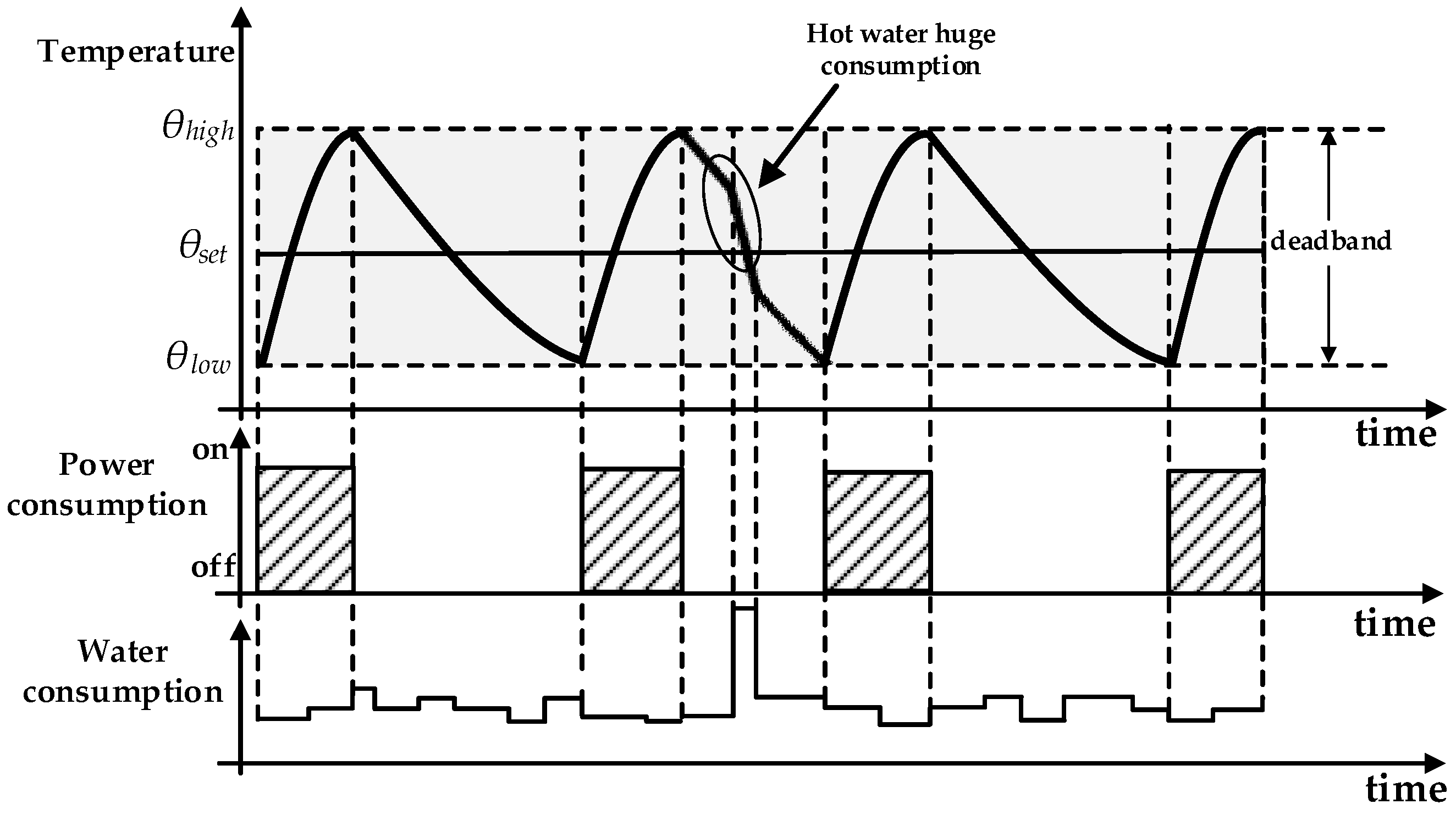
As shown in Figure 1, the temperature in the tank develops between ${\theta }_{high}$ and ${\theta }_{low}$. ${\theta }_{set}$ represents the setpoints of the water heater. When the water heater is on, the temperature increases along with power consumption, while when the water heater is off, it decreases. The curve in the ellipse simulates the temperature trend when the user demands a large quantity of hot water. The shaded rectangles below represent the power consumption. There is a unique correspondence between the temperature rising and the power consumption. The relationship of ${\theta }_{high}$, ${\theta }_{low}$, ${\theta }_{set}$, and $\delta$ can be defined as follows:

$$\{\begin{array}{c}{\theta }_{high}={\theta }_{set}+\frac{\delta }{2}\\ {\theta }_{low}={\theta }_{set}-\frac{\delta }{2}\\ \delta ={\theta }_{high}-{\theta }_{low}\end{array}$$

(2)

2.2. Efficient Power Plant Consisting of Water Heaters

Based on the single water heater’s thermal dynamic process, a group of water heaters can be regarded as an efficient power plant (EPP). Its output power limits $P_{min}^{t+\Delta t}$, $P_{max}^{t+\Delta t}$ at $t+\Delta t$, can be described as follows:

$$\{\begin{array}{l}{P}_{min}^{t+\Delta t}\le P_{EPP}^{t+\Delta t}\le P_{max}^{t+\Delta t}\\ P_{max}^{t+\Delta t}=P_{EPP}^t+{\displaystyle \sum P_{wh}^i}({\theta }^{i,t+\Delta t}\in ({\theta }_{low}^{i,t+\Delta t},{\theta }_{high}^{i,t+\Delta t}),u^{i,t}=0)\\ P_{min}^{t+\Delta t}=P_{EPP}^t-{\displaystyle \sum P_{wh}^i}({\theta }^{i,t+\Delta t}\in ({\theta }_{low}^{i,t+\Delta t},{\theta }_{high}^{i,t+\Delta t}),u^{i,t}=1)\end{array}$$

(3)

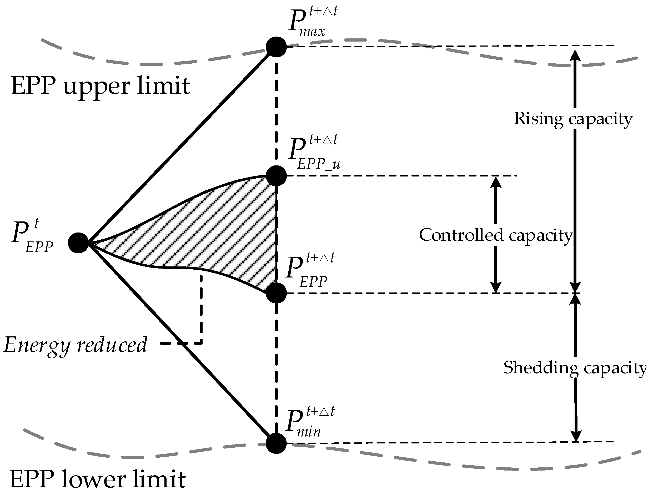
In Figure 2, the shaded triangle represents the energy reduced as a result of adopting control strategies during the period $\Delta t$, the gray dotted lines represent the EPP’s output limit, and the dark points are some possible operating status.

There are four main parameters: $P_{max}^t$ and $P_{min}^t$, which are logically equivalent to the users’ comfortable level constraints; uncontrolled EPP state $P_{EPP\_u}^t$; and controlled EPP state $P_{EPP}^t$. From Figure 2, it can be observed that if EPP-WH has a large feasibility range, and the operating point is near the upper limit, it has better conditions to become a good candidate for load shedding. Using these basic parameters, other main technical parameters can be defined as:

$$\{\begin{array}{l}\Delta P_{EPP}^{t+\Delta t}=P_{EPP}^{t+\Delta t}-P_{EPP\_u}^{t+\Delta t}\\ \Delta P_{up}^{t+\Delta t}=P_{max}^{t+\Delta t}-P_{EPP}^{t+\Delta t}\\ \Delta P_{down}^{t+\Delta t}=P_{min}^{t+\Delta t}-P_{EPP}^{t+\Delta t}\end{array}$$

(4)

The controlled capacity $\Delta P_{EPP}^{t+\Delta t}$ represents the capacity of the energy storage or the energy releasing capacity, that is to say that water heaters can absorb or release energy when the EPP-WH is under control; $\Delta P_{up}$ and $\Delta P_{down}$ represent the feasible regions of the EPP’s state, which are the feasible boundaries of the energy storage or the energy releasing capacity at this moment. In particular, the shedding capacity $\Delta P_{down}$ represents the EPP’s biggest power saving ability.

2.3. Lock On and Off Constraints

To prevent water heaters from being controlled too often, lock-on and off functions were included in the TPL [28] strategy. The basic logic of this constraint is to set minimum time limits $t_{limit}^{on}$ or $t_{limit}^{off}$. When a water heater is on or off, it should maintain its status for at least $t_{limit}^{on}$ or $t_{limit}^{off}$. The water heaters in lock-on and off status should not be controlled. Using parameter $l_{on}^{i,t}$ and $l_{off}^{i,t}$ as controlling index, using $t{r}_{on}^{i,t+1}$ and $t{r}_{off}^{i,t+1}$ as lock-on and off timer to record the lock time:

$$\{\begin{array}{ll}t{r}_{on}^{i,t+1}=t{r}_{on}^{i,t}+1& (l_{on}^{i,t}=1)\\ t{r}_{on}^{i,t+1}=0& (l_{on}^{i,t}=0)\\ t{r}_{off}^{i,t+1}=t{r}_{off}^{i,t}+1& (l_{off}^{i,t}=1)\\ t{r}_{off}^{i,t+1}=0& (l_{off}^{i,t}=0)\end{array}$$

(5)

$$l_{on}^{i,t}=\{\begin{array}{ll}1& t{r}_{on}^{i,t}<t_{limit}^{on},t{r}_{on}^{i,t}\ne 0\\ 0& t{r}_{on}^{i,t}\ge t_{limit}^{on}\end{array}$$

(6)

$$l_{off}^{i,t}=\{\begin{array}{ll}1& t{r}_{off}^{i,t}<t_{limit}^{off},t{r}_{off}^{i,t}\ne 0\\ 0& t{r}_{off}^{i,t}\ge t_{limit}^{off}\end{array}$$

(7)

If a water heater is being locked, the timer will keep counting, and during this period, EPP-WH cannot be controlled. After the timer reaches its time limits, the EPP-WH can be available again as shown in Equations (5)–(7). When calculating the limits of EPP-WH, Equation (3) needs to be updated:

$$\{\begin{array}{l}{P}_{min\_l}^{t+\Delta t}\le P_{EPP\_l}^{t+\Delta t}\le P_{max\_l}^{t+\Delta t}\\ P_{max\_l}^{t+\Delta t}=P_{EPP\_l}^t+{\displaystyle \sum P_{wh,i}}({\theta }^{i,t+\Delta t}\in ({\theta }_{low}^{i,t+\Delta t},{\theta }_{high}^{i,t+\Delta t}),u^{i,t}=0,l_{on}^{i,t}=0)\\ P_{min\_l}^{t+\Delta t}=P_{EPP\_l}^t-{\displaystyle \sum P_{wh,i}}({\theta }^{i,t+\Delta t}\in ({\theta }_{low}^{i,t+\Delta t},{\theta }_{high}^{i,t+\Delta t}),u^{i,t}=1,l_{on}^{i,t}=0)\end{array}$$

(8)

The controlled capacity $P_{EPP\_\mathrm{l}}^{t+\Delta t}$ represents the capacity of the energy storage or the energy releasing capacity, that is to say that water heaters can absorb or release energy when the EPP-WH is under control; $\Delta P_{up}$ and $\Delta P_{down}$ represent the feasible regions of the EPP’s state, which are the feasible boundaries of the energy storage or the energy releasing capacity at this moment. In particular, the shedding capacity $\Delta P_{down}$ represents the EPP’s biggest power saving ability:

$$\{\begin{array}{l}\Delta P_{EPP\_l}^{t+\Delta t}=P_{EPP\_l}^{t+\Delta t}-P_{EPP\_u}^{t+\Delta t}\\ \Delta P_{up\_l}^{t+\Delta t}=P_{max\_l}^{t+\Delta t}-P_{EPP\_l}^{t+\Delta t}\\ \Delta P_{down\_l}^{t+\Delta t}=P_{min\_l}^{t+\Delta t}-P_{EPP\_l}^{t+\Delta t}\end{array}$$

(9)

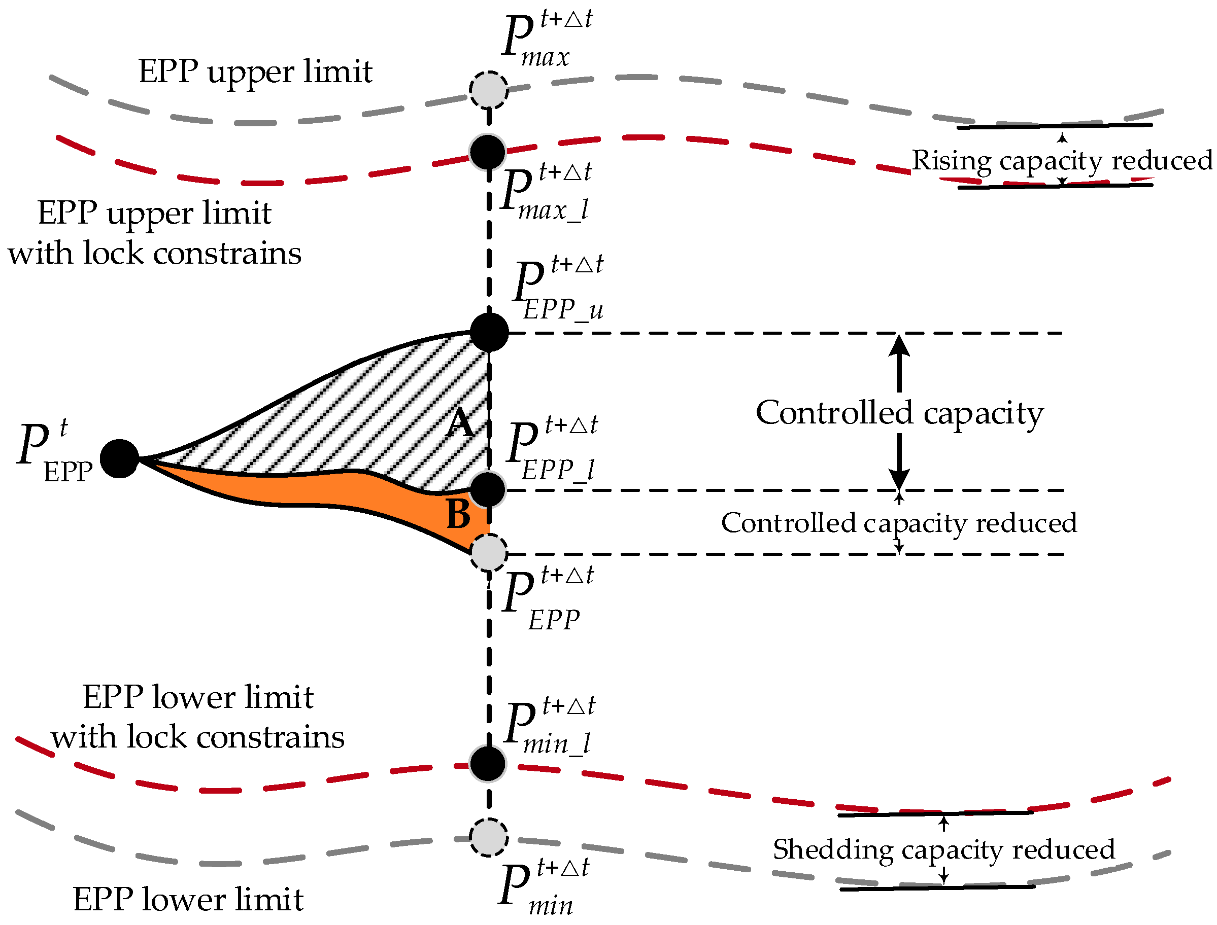
Figure 3 shows the operating points of the EPP-WH, where the gray points represent the state without lock-on and off constraints. The upper and lower limits of the EPP-WH have shrunk. Compared with the uncontrolled point $P_{EPP\_u}^t$, the total energy restored can be seen as Section A plus section B. Taking lock-on and off constraints into account, some water heaters cannot be controlled even if they are within reasonable temperature ranges. Therefore, the target generation of the EPP-WH is becoming “conservative”, leading to a higher operating point $\Delta P_{EPP\_l}^t$, and the energy restored decreased to only the area in section A. The load capacities of the rising, decreasing, and controlled were all reduced. But with this constraint, the users’ comfortable levels were maintained, which is a major advantage of this approach.

2.4. Users’ Willingness Model

Users’ willingness $\gamma$ can be defined as the degree of initiative for water heater users to participate into demand response. It is affected by many factors, like educational level, family income, family members’ age [29,30] and so on. Generally, family members having a college or above education level have stronger willingness to participate in demand response; families with higher income increase their initiative; if the average age of family members is between 35–45, it is more likely to have a strong willingness to participate in demand response. In this part, three factors—educational level, income influence and family members’ age—are taken into account. 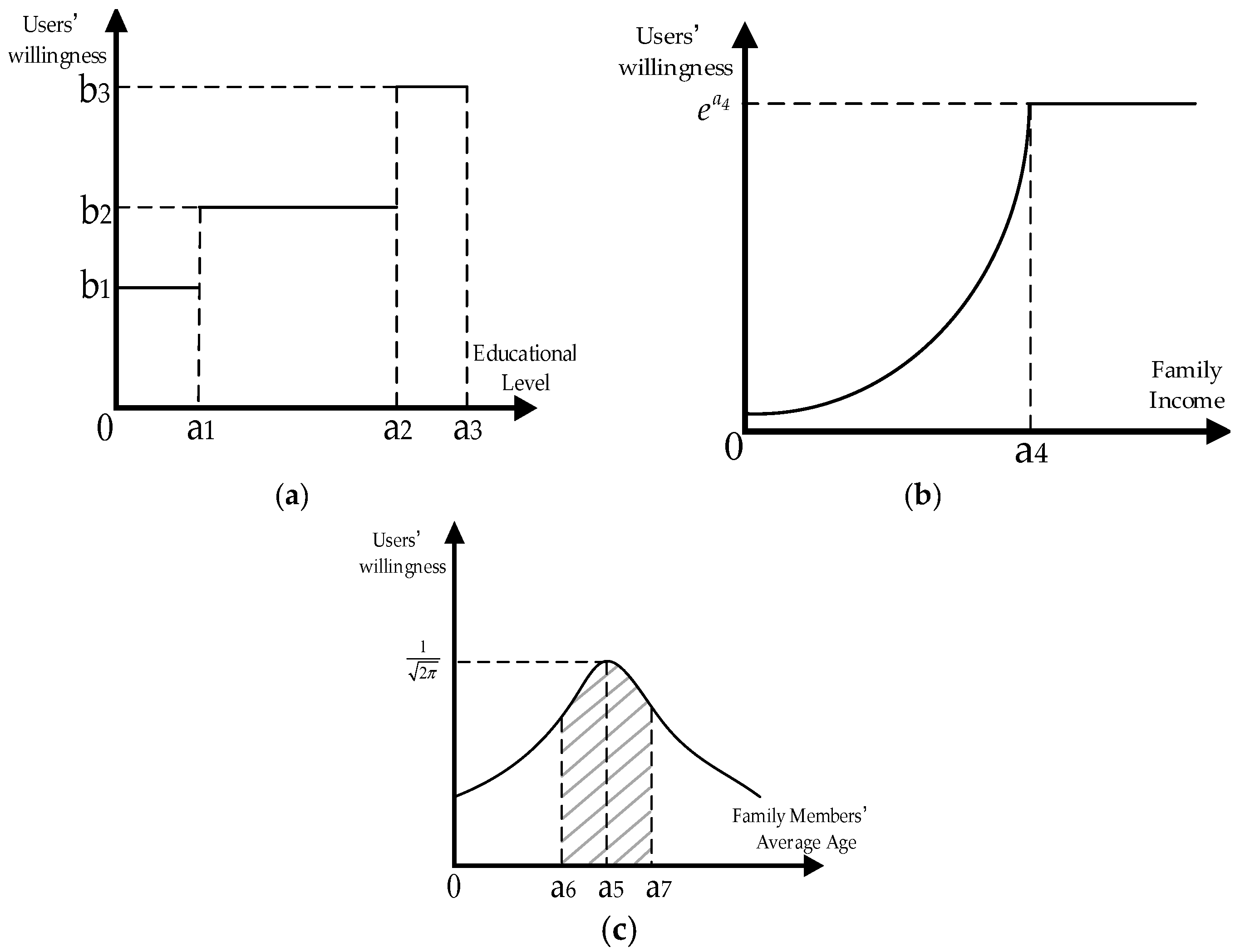Figure 4 shows the relationship of related factors and uses’ willingness. As the diversity of educational level is not as abundant as that of family income and family members’ age, three levels are set up to describe the influences of educational level on users’ willingness, $EL$ stands for the education level.

$$\begin{array}{l}{\gamma }_{EL}=\{\begin{array}{ll}{b}_1& 0<EL\le a_1\\ b_2& a_1<EL\le a_2\\ b_3& a_2<EL\le a_3\end{array}\end{array}$$

(10)

The low and middle income group account for the majority of the total group. This group of people have relatively weaker willingness to participate in demand response activities compared with the high income group, so an exponential model is set up to describe the influence of educational level on users’ willingness. Here $FI$ stands for the family income:

$$\begin{array}{l}{\gamma }_{FI}=\{\begin{array}{cc}{e}^{FI}\hfill & 0<FI\le a_4\\ e^{a_4}\hfill & FI>a_4\end{array}\end{array}$$

(11)

where $a_4$ stands for the maximum input, if $FI$ is more than $a_4$, the influence stays the same.

The influence of family members’ average age on users’ willingness can be described as follows:

$$\begin{array}{l}{\gamma }_{FA}=\frac{1}{\sqrt{2\pi }}{e}^{(-\frac{{(FA-a_5)}^2}{2{\sigma }^2})}\end{array}$$

(12)

The influences of family members’ average age obey a normal distribution with expectation $a_5$ and standard deviation $\sigma$, which means children and the aged are not the main participants in demand response programs. People aged between $a_6$ and $a_7$ (usually 35–45) will have more interest.

Based on the analysis above, an integrated users’ willingness model can be set up:

$${\gamma }_{wh}=\frac{{\gamma }_{EL}\cdot {\gamma }_{FI}\cdot {\gamma }_{FA}}{max({\gamma }_{EL}\cdot {\gamma }_{FI}\cdot {\gamma }_{FA})}$$

(13)

where ${\gamma }_{wh}$ has taken educational level, family income and family members’ average age into account. ${\gamma }_{wh}$ changes from 0 to 1 after normalization.

3. Optimization and Strategies

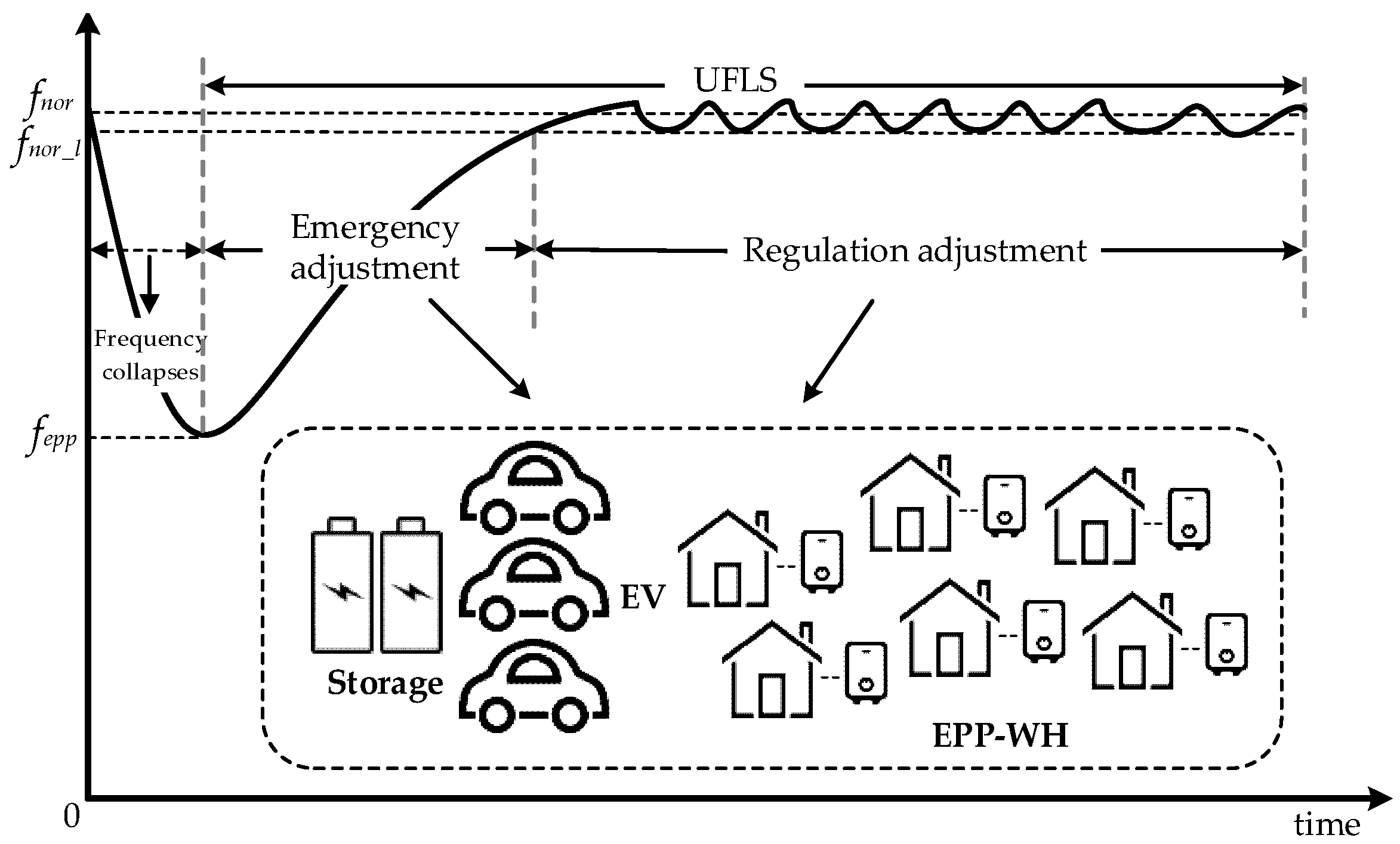
This section will discuss the main optimization methods and strategies. Figure 5 illustrates the different periods of frequency response and the corresponding resources. When the system is running normally, the frequency of the system is kept within a reasonable range, which is usually a ±0.2 Hz deviation of the system standard frequency (50 or 60 Hz). When there is a system disturbance, the frequency of the system may immediately drop out of the normal range. The first part of the UFLS will begin when the system frequency is below $f_{epp}$; this part can be regarded as “emergency adjustment”, which undertakes the most load shedding task, with the EPP-WH, EV, and storage (such as batteries) as the frequency response resources.

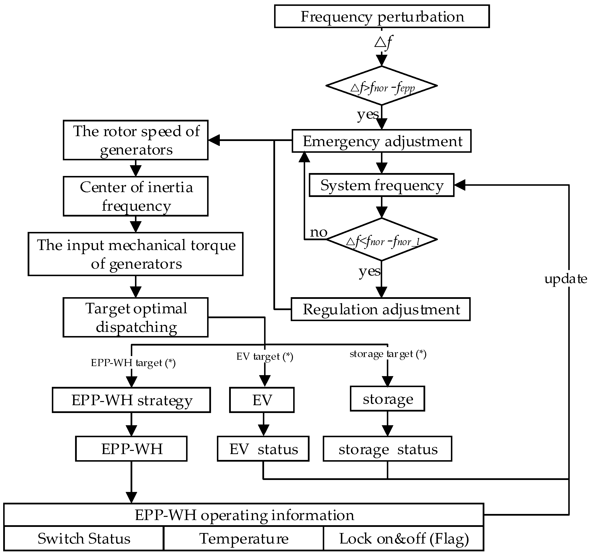
When the frequency changes back to $f_{nor\_l}$, which is the lower limit of the system frequency, regulation adjustment begins in order to maintain the system frequency. A long-term approach will be implemented, which includes load shedding and rising, different from the emergency adjustment. Figure 6 illustrates the control structure and strategies.

By analyzing the status of the generators, the frequency deviation of the system $\Delta f$ and the required load to be shed $\Delta P$ can be calculated. With the evaluation of $\Delta f$, the frequency response resource will be decided. Using information on the generator’s operating point, the total target $\Delta P$ can be calculated through a series of analyses which will be elaborated in more detail in the following section. The EPP-WH, EV, and storage receive their targets based on their percent power consumption in the system. In this study, we focused on the performance of the EPP-WH, assuming EV and storage has good and stable performance. To ensure that appropriate targets are dispatched, several elements were taken into account, including the EPP-WH “users’ willingness” and operating points. During the period of emergency adjustment, each type of resources decreases its power consumption to help pull the system frequency back to the normal range. While in the regulation adjustment period, response targets generated from the system includes both load increasing and load shedding.

3.1. Load Shedding Calculation

When a disturbance occurs in a multi-machine power system, with the measured dynamic system response, changes in rotor speed of synchronous generators can be detected first. In the process of dynamic frequency change, different generators have different influences on the system frequency. Therefore, the definition of the center of inertia (COI) frequency is put forward. In this paper, the rate of change of the COI frequency is regarded as the rate of change of the system frequency. Based on this, the rotor speed and the motion equation of the COI are expressed as follows:

$$\{\begin{array}{l}{\omega }_{COI}=\frac{1}{T_J}{\displaystyle \sum _{i=1}^N{T}_{J_i}{\omega }_i}\\ T_J\frac{\mathrm{d}{w}_{COI}}{\mathrm{d}t}=\Delta P\end{array}$$

(14)

where ${\omega }_{COI}$ is the rotor speed of the center of inertia (rad/s), $T_J={\displaystyle \sum _{i=1}^N{T}_{J_i}}$, $T_{J_i}$ is the input mechanical torque of the ith generator (kW·s·rad⁻¹), $f_{\mathrm{COI}}$ is the frequency of the center of inertia (Hz) based on the relationship ${\omega }_{COI}=2\pi f_{COI}$, in per unit value, ${\omega }_{COI}=f_{COI}$:

$$\{\begin{array}{l}{f}_{COI}=\frac{1}{T_J}{\displaystyle \sum _{i=1}^N{T}_{J_i}{f}_i}\\ T_J\frac{\mathrm{d}{f}_{COI}}{\mathrm{d}t}=\Delta P\end{array}$$

(15)

Using Equation (15), the target load shedding $\Delta P$ is achieved. Using information on water heater users’ willingness and the operating point, $f_{epp}$ can be obtained as:

$$\{\begin{array}{c}{f}_{epp}=f_{nor}-\gamma \times f_P\\ {\gamma }^i={\displaystyle \sum _{k=1}^{N^i}{\gamma }_{wh}^{i,k}}\times \frac{P_{wh}^{i,k}}{P_{EPP}^i}\\ \gamma ={\displaystyle \sum _{i=1}^m{\gamma }^i}\times \frac{P_{EPP}^i}{P_{EPP\_total}^i}\\ P_{EPP\_total}^i={\displaystyle \sum _{i=1}^m{P}_{EPP}^i}\end{array}$$

(16)

where ${\gamma }_{wh}^{i,k}$ stands for the kth water heater user’s willingness in the i-th EPP-WH, ranging from 0 to 1, $P_{wh}^{i,k}$ is the power consumption of the k-th water heater. ${\gamma }^i$ can be calculated through a method of weighting considering users’ actual power consumption, and $\gamma$ can be generated by weighting all the ${\gamma }^i$ in system. $f_P$ represents the maximum frequency range of the regulation frequency adjustment, which can be estimated by Equation (16). Using information from the system, appropriate targets can be identified to the execution units under different $\Delta f$ conditions. Equation (15) describes the relationship between the rate of frequency and the loads that need to be decreased or increased. Before the frequency returns back to $f_{nor\_l}$, $\Delta P$ is a negative parameter; during this emergency adjustment period, the system continues load shedding. While in the regulation adjustment process, $\Delta P$ may be a positive or negative parameter depending on the system operating status, the system has demands of shedding and increasing loads.

3.2. Target Assignment Method

Assuming there is a load shedding demand at time t, the EPP-WHs at higher operating points will be suitable to undertake more task, as they have larger $\Delta P_{down}$ to decrease their power consumption. Similarly, if one EPP-WH is operating at a lower point, it can be a good resource to response load rising target. To evaluate the influences of EPP-WH’s operating status, parameter $\lambda$ is defined to calculate the degree of suitability for an EPP-WH to participate into demand response. $\lambda$ can be obtained through analysis of the operating status of EPP-WH. Considering the lock-on effects and diversities of EPP-WHs, each EPP-WH has different operating status and power limits which are all time-varying, the degree of suitability for an EPP-WH to participate into demand response at time t can be defined as follows:

$${\lambda }^{k,t}=\{\begin{array}{ll}\Delta P_{up\_l}^t/(P_{max\_l}^t-P_{min\_l}^t)& \mathrm{load}\mathrm{shedding}\\ \Delta P_{down\_l}^t/(P_{max\_l}^t-P_{min\_l}^t)& \mathrm{load}\mathrm{rising}\end{array}$$

(17)

Conclusion can be drawn that the larger the value of ${\lambda }^{k,t}$ is, the more targets should be distributed to this EPP-WH, and the more ith EPP-WH is likely to be a good response resource. Based on the analysis above, the objective function and constraints can be written as follows:

$$\begin{array}{l}obj\min \{{\displaystyle \sum _{k=1}^m(1-{\lambda }^{k,t})|\Delta P^{*k,t}|}\}\\ st{\displaystyle \sum _{k=1}^m\Delta P^{*k,t}}=\Delta P_{total}^t\\ \{\begin{array}{ll}\Delta P_{down\_l}^{t+\Delta t}<\Delta P^{*k,t}<0& \mathrm{load}\mathrm{shedding}\\ 0<\Delta P^{*k,t}<\Delta P_{up\_l}^{t+\Delta t}& \mathrm{load}\mathrm{rising}\end{array}\end{array}$$

(18)

where $\Delta P^{*k,t}$ stands for the target distributed to ith EPP-WH, $\Delta P_{total}^t$ is the total target which can be generated by Equation (15). The equation constraint means all the EPP-WHs undertake the total target $\Delta P_{total}^t$. Besides, every EPP-WH should satisfy its upper and lower limits considering the lock-on and off effects. By using $1-{\lambda }^{k,t}$ as weighting factor, the target generated from objective function has considered the influences of users’ willingness ${\lambda }^{k,t}$ and the lock-on and off constraints. Using PSO method to solve this optimal problem, generating $\Delta P^{*k,t}$ for each EPP-WH.

3.3. EPP-WH Optimization Strategies

In this study, a new TPL method with lock-on and off constraints was used to control the EPP-WH.

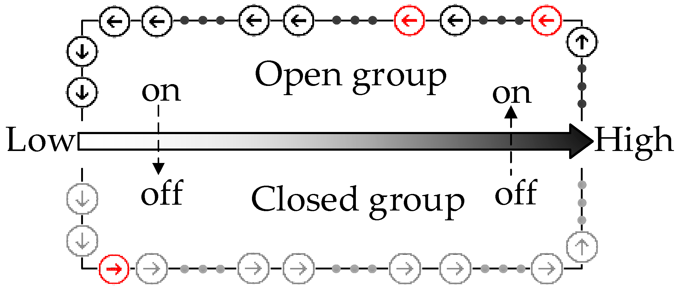
First, at each time step, taking into account the status of the water heaters, the controlled group were screened out, the upper and lower limits were calculated using Equation (3), the EPP-WH was developed, in which water heaters in “lock” status have been eliminated. Second, the water heaters were divided into two parts based on their switch’s status, making up two controlled groups as shown in Figure 7 and Equations (19)–(20):

$${\mathbf{O}}_{open}^t=(O_1^t,O_2^t,O_3^t,\dots ,O_{n_1}^t),$$

(19)

$${\mathbf{C}}_{closed}^t=(C_1^t,C_2^t,C_3^t,\dots ,C_{n_2}^t).$$

(20)

In ${\mathbf{O}}_{open}^t$, water heaters were sorted according to their temperature in descending order. While in ${\mathbf{C}}_{closed}^t$, water heaters were sorted according to their temperature in ascending order.

In Figure 7, the temperature increases from left to right, the dark arrows represent water heaters in the ${\mathbf{O}}_{open}^t$ at the time t, the gray arrows represent those in the ${\mathbf{C}}_{closed}^t$, and the red arrows represent water heaters eliminated from the EPP-WH. All the arrows move in the clockwise direction, the water heaters at the end of each group will switch their status automatically and step into the other group at the next time step.

Finally, a group of water heaters will be turned off or turned on, that is to say, the EPP-WH decreases or increases the power consumption by a certain amount based on the type of targets sent to it. When the EPP-WH has to decrease its power consumption, the exact number of the water heaters to be turned off can be calculated by:

$$\{\begin{array}{l}{\displaystyle \sum _{i=1}^{ko+1}{P}_{wh,i}}\ge P_{EPP\_l}^t-\Delta P^{k,t}\\ {\displaystyle \sum _{i=1}^{ko}{P}_{wh,i}}<P_{EPP\_l}^t-\Delta P^{k,t}\end{array}$$

(21)

Then the top $ko$ water heaters in the ${\mathbf{O}}_{open}^t$ will be closed, and the EPP-WH decreases its power consumption for $\Delta P^{k,t}$. Similarly, when the EPP-WH has to increase its power consumption, the exact number of the water heaters to be turned on can be calculated by:

$$\{\begin{array}{l}{\displaystyle \sum _{i=1}^{kc+1}{P}_{wh,i}}\ge P_{EPP\_l}^t-\Delta P^{k,t}\\ {\displaystyle \sum _{i=1}^{kc}{P}_{wh,i}}<P_{EPP\_l}^t-\Delta P^{k,t}\end{array}$$

(22)

Then the top $kc$ water heaters in the ${\mathbf{C}}_{closed}^t$ will be opened, and the EPP-WH increases its power consumption for $\Delta P^{k,t}$.

4. Simulation Results and Analysis

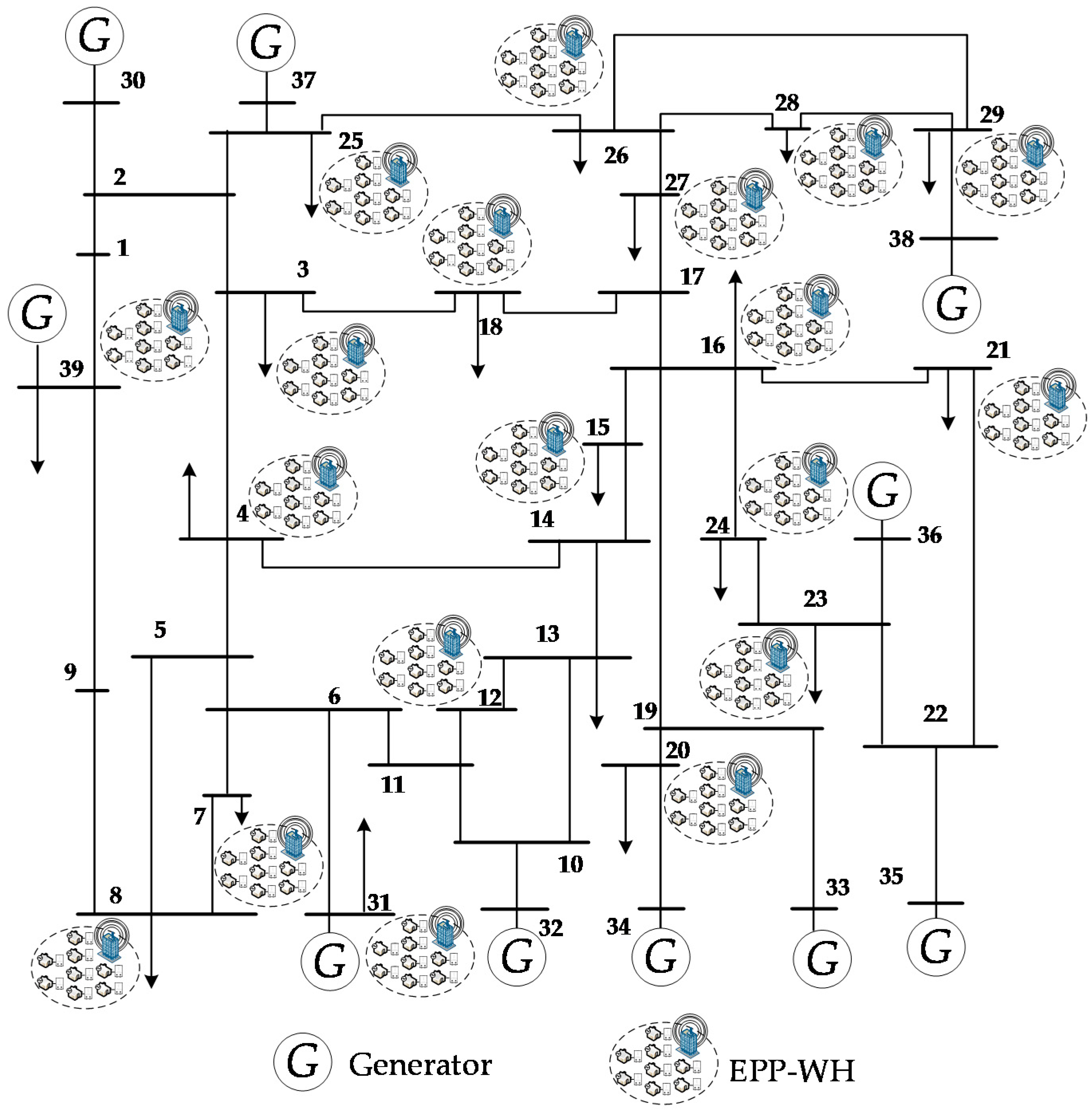
This section discusses the effects of several key parameters on the control methods. All the cases are based on the IEEE New England 10 generators 39 bus system. Figure 8 shows the topology of the system, while the active power of the load nodes are listed in

Table 1. Active power of load nodes.

Bus-ID	Active Power (MW)	Water Heater Number	Total Water Heater Power Capacity (MW)
3	322	5240	31.4
4	500	8180	49.1
7	233.8	3800	22.8
8	522	8490	50.9
12	8.5	140	0.84
15	320	5240	31.4
16	329	5350	32.1
18	158	2570	15.4
20	680	11,060	66.4
21	274	4450	26.7
23	247.5	4020	24.1
24	308.6	5020	30.1
25	224	3640	21.8
26	139	2260	13.6
27	281	4560	27.4
28	206	3350	20.1
29	283.5	4610	27.7
31	9.2	150	0.9
39	1104	17,870	107.2
Total	6150.1	100,000	600

. The total number of water heaters was 100,000 with an average power 6 kW. Assuming a smart controlling unit has been set, the control period of the EPP-WH was 10 s. A detailed description of the system is presented in the Appendix A. 3-order model was used to describe the status of the generators, the detailed parameters are presented in

Table A1. Generator parameters.

No.	${\mathit{x}}_{\mathit{d}}^{\prime }$ (pu)	${\mathit{x}}_{\mathit{q}}^{\prime }$ (pu)	${\mathit{x}}_{\mathit{d}}$ (pu)	${\mathit{x}}_{\mathit{q}}$ (pu)	${\mathit{T}}_{\mathit{d}0}^{\prime }$ (s)	${\mathit{T}}_{\mathit{q}0}^{\prime }$ (s)	${\mathit{x}}_{\mathit{l}}$ (pu)
1	0.006	0.008	0.02	0.019	7	0.7	0.003
2	0.0697	0.17	0.295	0.282	6.56	1.5	0.035
3	0.0531	0.0876	0.2495	0.237	5.7	1.5	0.0304
4	0.0436	0.066	0.262	0.258	5.69	1.5	0.0295
5	0.032	0.166	0.67	0.62	5.4	0.44	0.054
6	0.05	0.0814	0.254	0.241	7.3	0.4	0.0224
7	0.049	0.086	0.295	0.292	5.66	1.5	0.0322
8	0.057	0.0911	0.29	0.28	6.7	0.41	0.028
9	0.057	0.0587	0.2106	0.205	4.79	1.96	0.0298
10	0.091	0.008	0.1	0.069	10.2	0	0.0125

, the detailed slack generator parameters are listed below in

Table A2. Slack Generator data.

Data	Description	Unit
31	Bus number	int
100.0	Power rating	MVA
100.00	Voltage rating	kV
0.98200	Voltage magnitude	p.u.
0.00000	Reference Angle	p.u.
9999.00000	Maximum reactive power	p.u.
−999.90000	Minimum reactive power	p.u.
1.1	Maximum voltage	p.u.
0.9	Minimum voltage	p.u.
5.72835	Active power guess	p.u.
1	Loss participation coefficient	-
1	Reference bus	-
1	Connection status	-

.

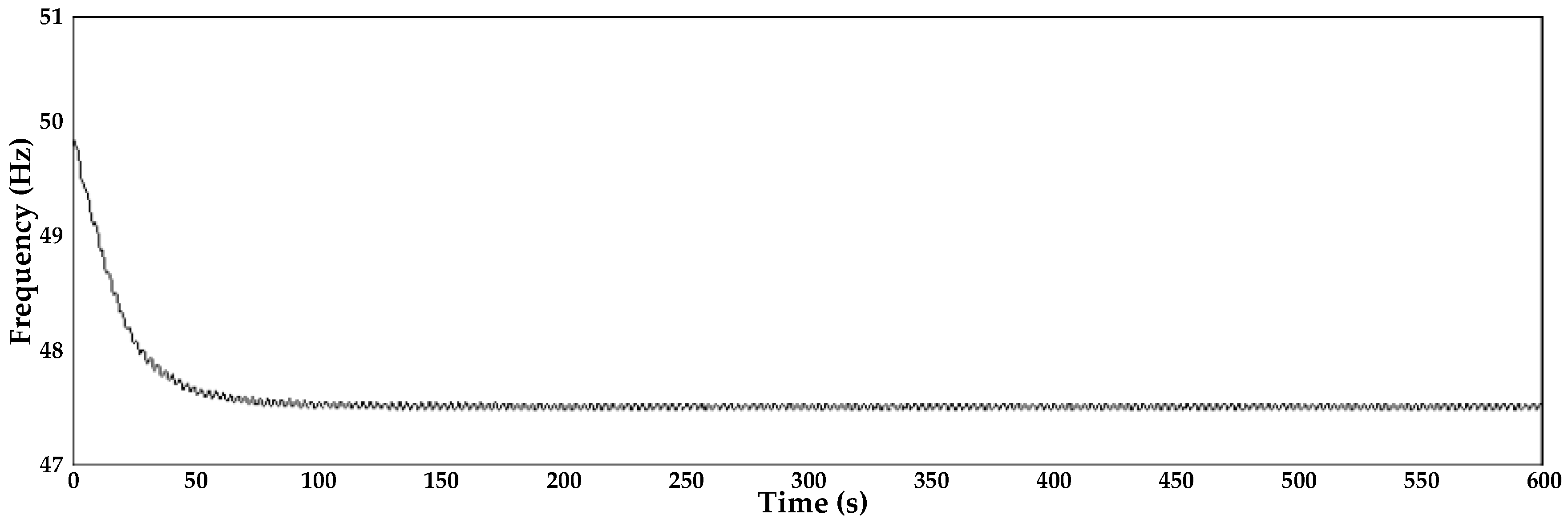
In this study, to achieve a drastic frequency change, the load level increased by 28% at the start of the simulation, and the system frequency quickly decreased to 47.6 Hz as shown in Figure 9.

4.1. Case 1-Principle of Traditional UFLS Method

The traditional method requires four or more rounds to undertake load shedding. During this period, different percentages of $\Delta P$ load shedding will be carried out. As the load shedding percent has been set previously, it cannot achieve accurate frequency adjustment. Besides, the multi-rounds schedule comes up with time delay, which should not be ignored. A typical load shedding schedule is presented in

Table 2. Load shedding schedule.

Round	Trigger Frequency (Hz)	Time Delay (s)	Load Shedding Percent (%)
1	49.25	0.2	30
2	49	0.2	30
3	48.75	0.2	20
4	48.5	0.2	20

.

4.2. Case 2-Comparision of Different UFLS Methods

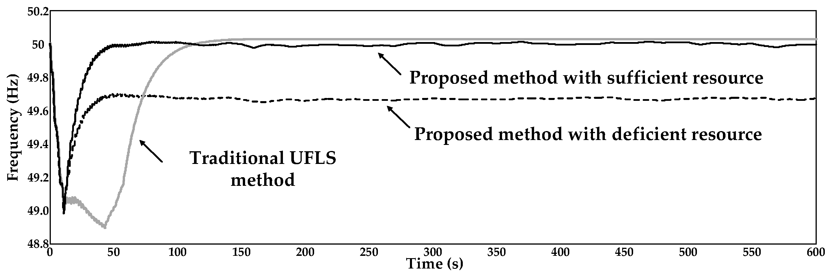
In this section, a comparison of different frequency adjustment strategies is presented to illustrate the advantages of the proposed method. The two strategies are under the same simulation conditions, three frequency curves are shown in Figure 10, which represent the traditional method, the proposed method with sufficient resource, and the deficient resource, respectively. It can be observed that the proposed method had a shorter reaction time and less frequency deviations from the $f_{nor}$. This is because using frequency response resources, such as the EPP-WH, EV, and storage, targets and commands are generated in real-time; therefore, the entire response process can be more generalized. As the EPP-WH has a quick response speed, the influences of time delay can be decreased. However, if the frequency adjustment resource is not sufficient, the response curve may remain in the lower level as shown in Figure 10.

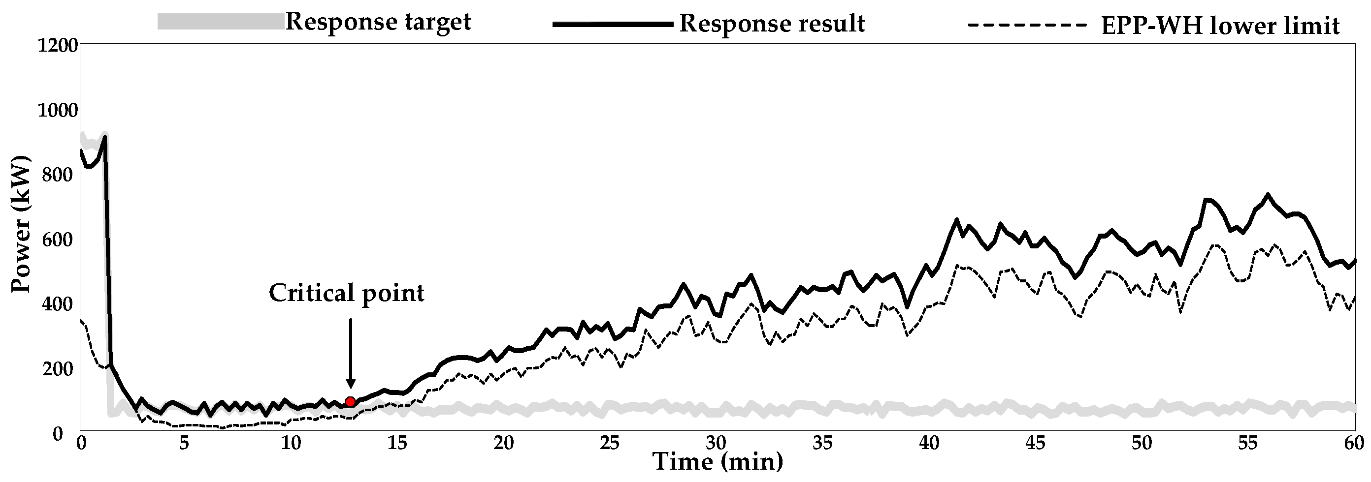
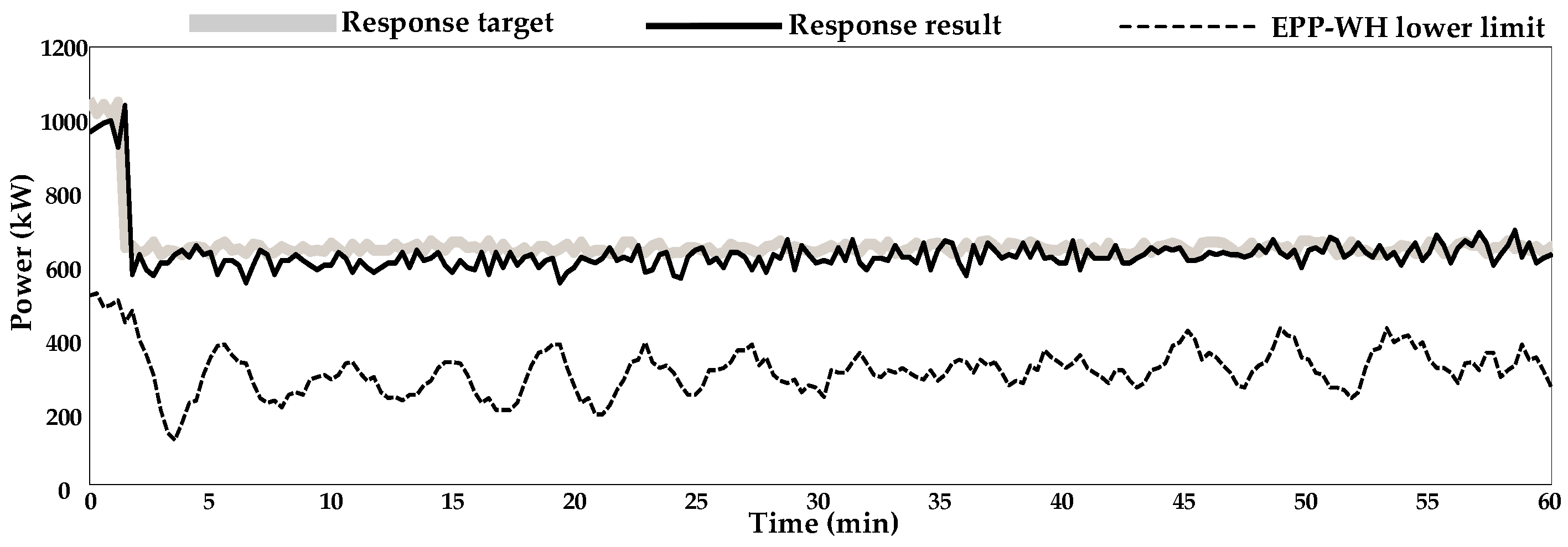
The EPP-WH power with deficient and sufficient resources are presented in Figure 11 and Figure 12. It was observed that only when the EPP-WH received a reasonable response target (within its response range), can the water heaters exhibit stable performance. If the target remains lower than the lower limit of the EPP-WH, a high number of water heaters will be switched on to maintain the users’ comfortable levels leading to a relatively large response error as shown in Figure 11. In this case, the critical point has divided the response process into two periods. In the beginning of a period of time, the EPP-WH had enough demand response resource to follow the target. While after the critical point, demand response resource decreased significantly. Since the number of water heaters in ${\mathbf{C}}_{closed}^t$ decreased over time, for a single water heater, being closed for a long time means that the water temperature will be continuously decreasing, more water heaters will switch on, and go into the ${\mathbf{O}}_{open}^t$ again to maintain the basic temperature demand. Therefore, a reasonable response target is of great importance for the comparison of Figure 11 and Figure 12.

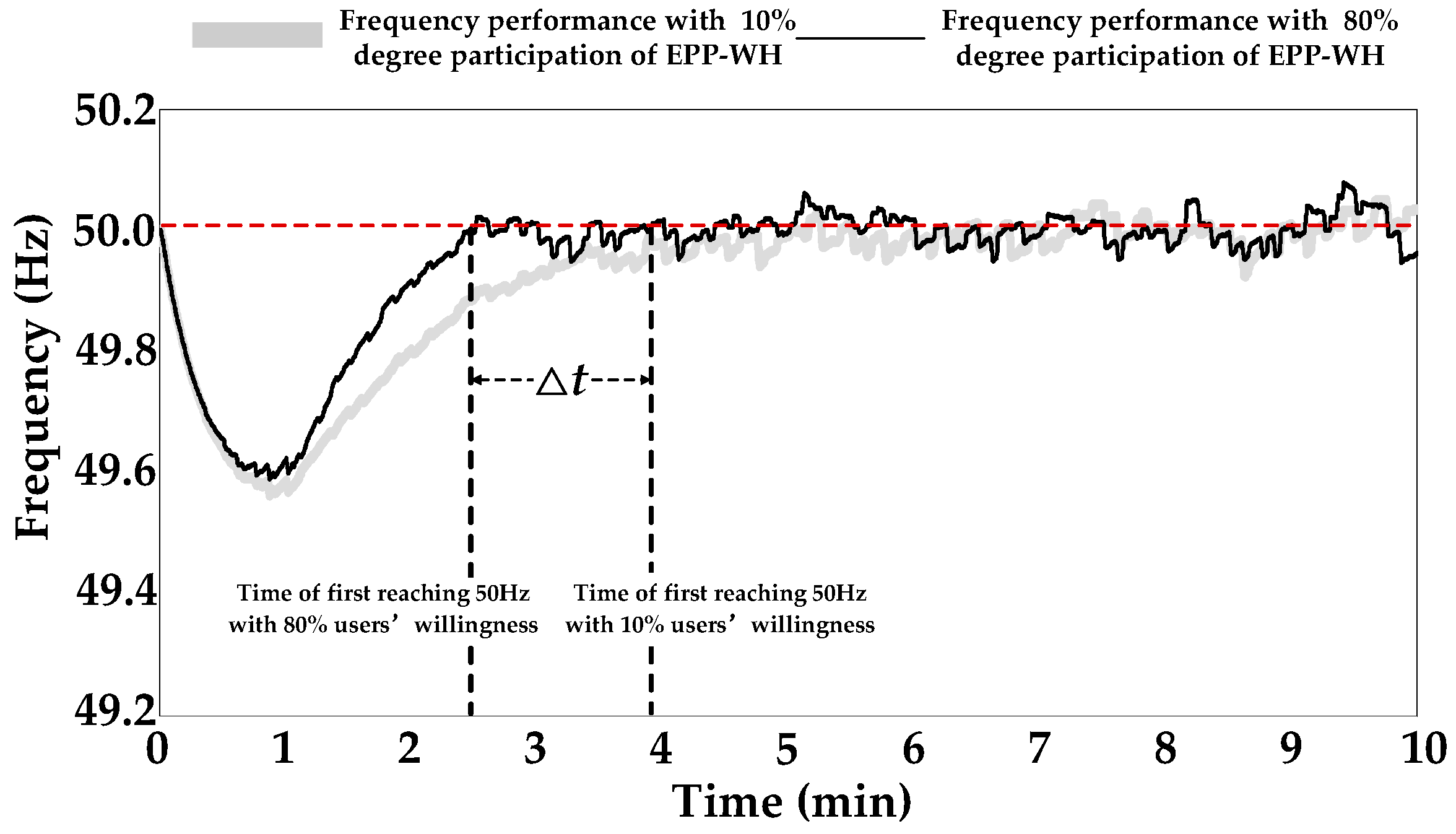
4.3. Case 3-Performance of EPP-WH Based on Different Water Heater Users’ Willingness

Figure 13 shows the EPP-WH’s performance of frequency regulation based on different users’ willingness: 10% and 80% degrees of participation of the EPP-WH were simulated. That is, 10% and 80% of all the water heater users agreed to be controlled during the period of demand response.

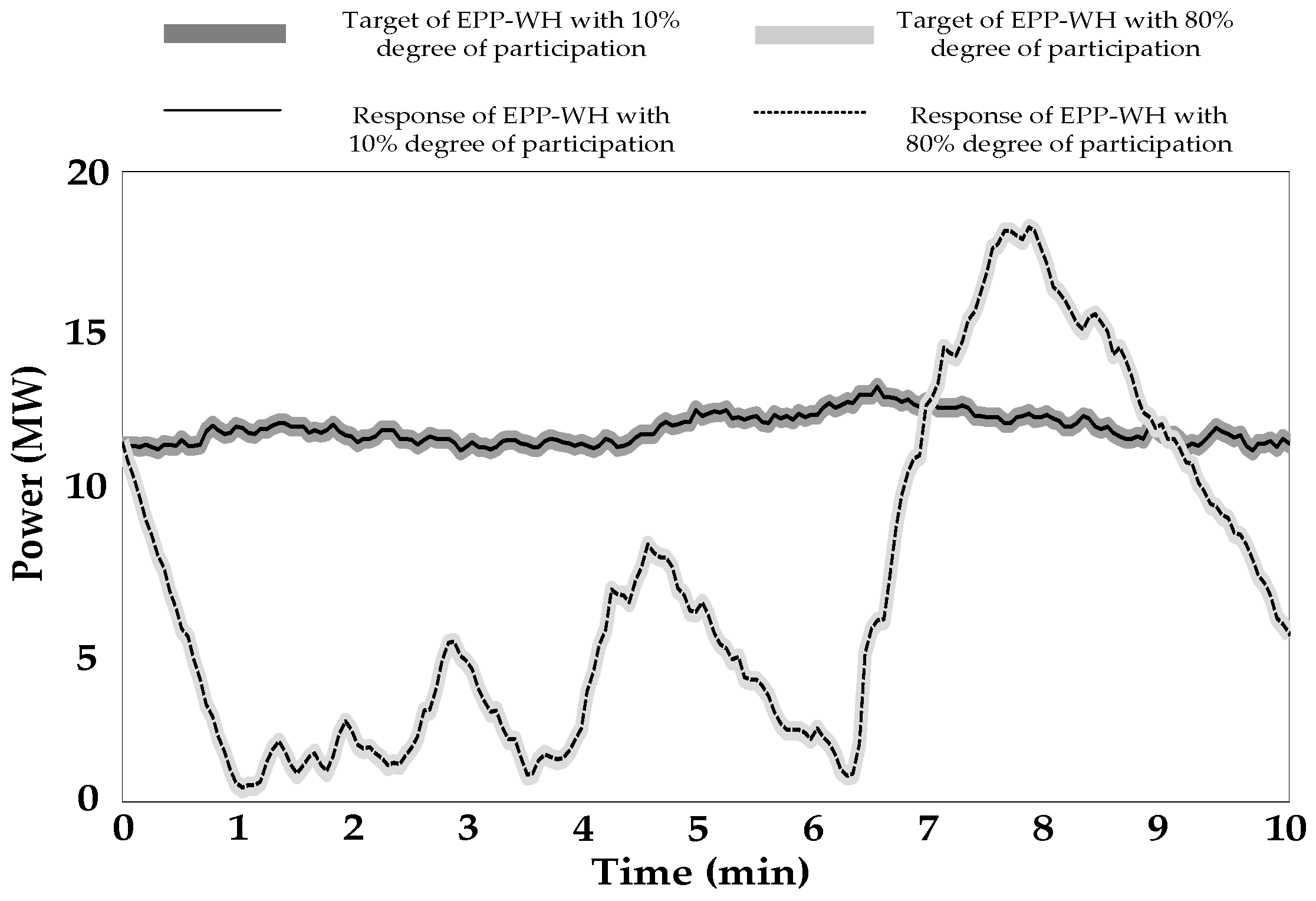
To study the effects of different users’ willingness independently, supplemental resources were forbidden. Considering the scale of the EPP-WH, appropriate targets were set. There is a time difference △t between the two curves first reaching a frequency of 50 Hz. It was observed that the more the users participate in the demand response, the less the time required for the recovery of system’s frequency. The normal range of frequency is 49.8–50.2 Hz in this case. At the beginning, a disturbance causes the frequency of the system to decrease from 50 Hz to approximately 49 Hz. After a time of 30 s, UFLS measures were implemented to prevent more severe frequency collapse. Targets were generated, and the EPP-WH responded to these targets by shedding a certain amount of loads. After a period of approximately 1 min, the trajectory of the frequency returned back to the normal range. Despite this, the willingness of the water heater users still had great effects on the targets sent to the EPP-WH as shown in Figure 14. From Figure 14, it can be observed that when the water heater users have stronger willingness to participate in load shedding, the top layer optimization module will send more targets to the EPP-WH. In the case of 80% degree of participation, the target increased after 6 min because most water heaters have already been turned off. To maintain the users’ comfortable levels, targets sent to the EPP-WH were adjusted, which also can be speculated, as the operating point was close to the lower limit of the EPP-WH.

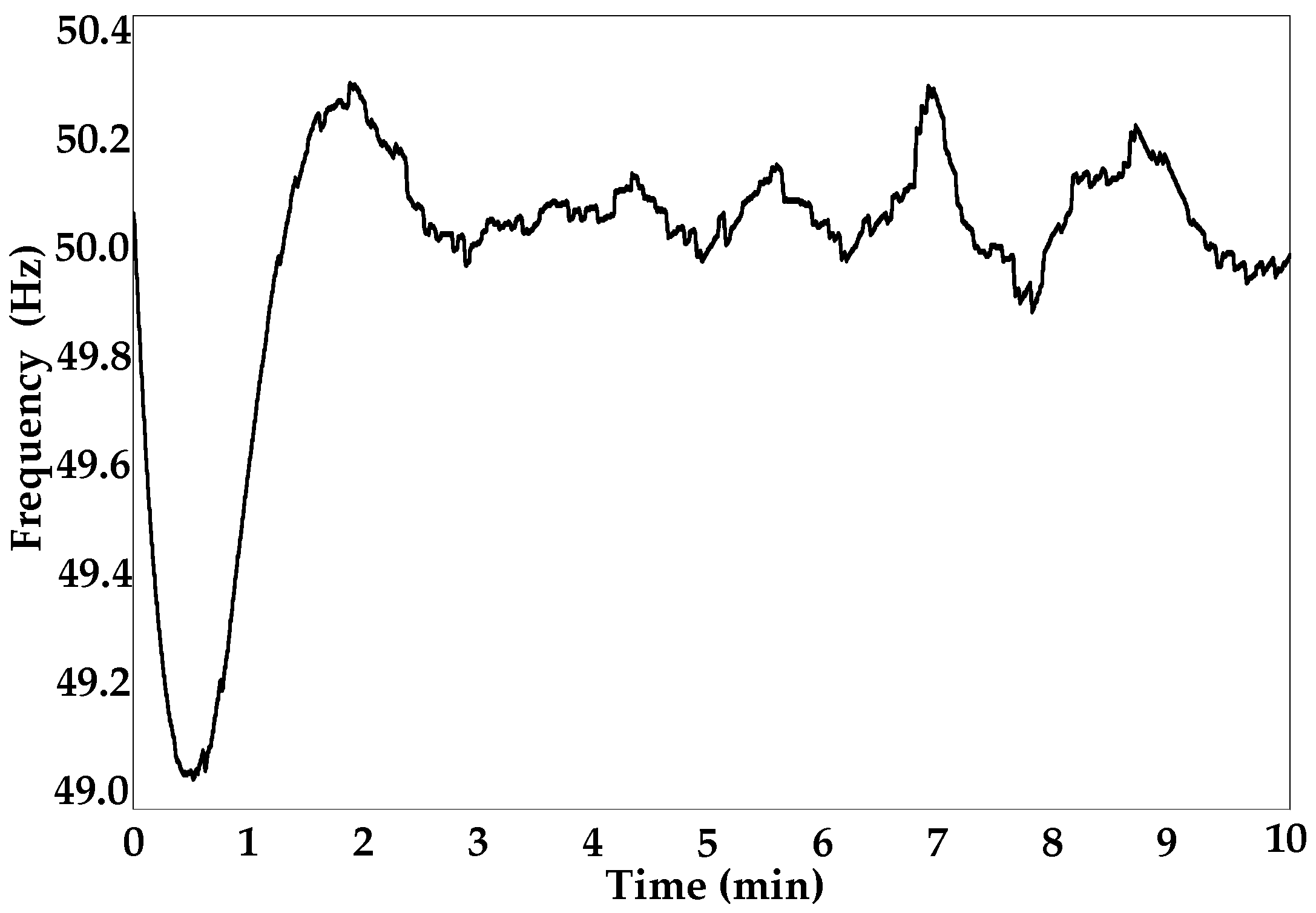
If the system does not have abundant supplemental resources, and the EPP-WH has a lower heater users’ willingness to participate in the demand response at the same time, the system will have little controllable resources, resulting in poor frequency performance as shown in Figure 15.

Therefore, a certain amount of supplemental resources are of great significance as the UFLS is not the only method for maintaining the system’s frequency. Therefore, alternative schemes should be anticipated.

4.4. Case 4-Influence of Lock-On and Off Constrains

On the one hand, the UFLS is a type of long-term method to maintain the normal status of power systems. On the other hand, water heaters should not be controlled too often when there are no urgent frequency regulation demand. The control period of the EPP-WH will be extended to 1 min after the normal period of system’s frequency. Figure 16 shows the EPP-WH’s operating in the upper and lower limits without lock-on and off constraints and the status taking constrains into consideration with a 5 min time limit.

The limits of the EPP-WH were significantly reduced due to the lesser availability of resources. Though the feasible region was smaller, this constraint was beneficial because the controlled time of each water heater per minute has decreased from 3.2 to 1.3, which improved the users’ comfortable levels. Therefore, appropriate lock-on and off constraints should be encouraged on the premise of acceptable response errors.

Figure 17 shows the frequency performance with and without the lock-on and off constraints. As presented above, with the support of supplemental resources, the system’s frequency has been maintained in a reasonable region.

4.5. Case 5-Temperature Changes of EPP-WH When Controlled

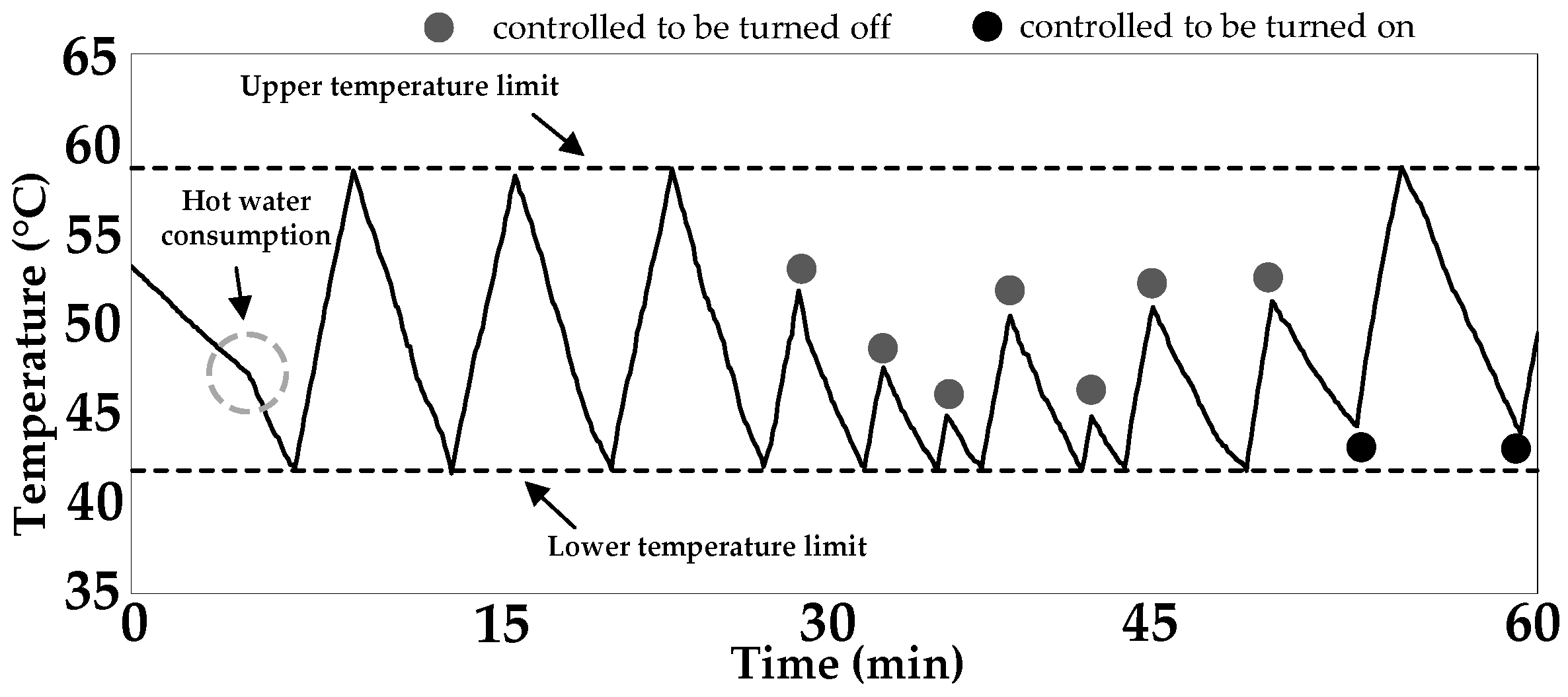
Figure 18 shows the behavior of a single water heater with 16 °C dead-band and 50 °C setpoint, according to Equation (2), the upper and lower temperature limits can be calculated. The circle with dashed line on the left highlights the obvious curve of the temperature trajectory indicating the moment when hot water was used, according to Equation (1). The gray points indicate the moment when the water heater received the command to be turned off, while the black points indicate the time measures were implemented to turn on the water heater.

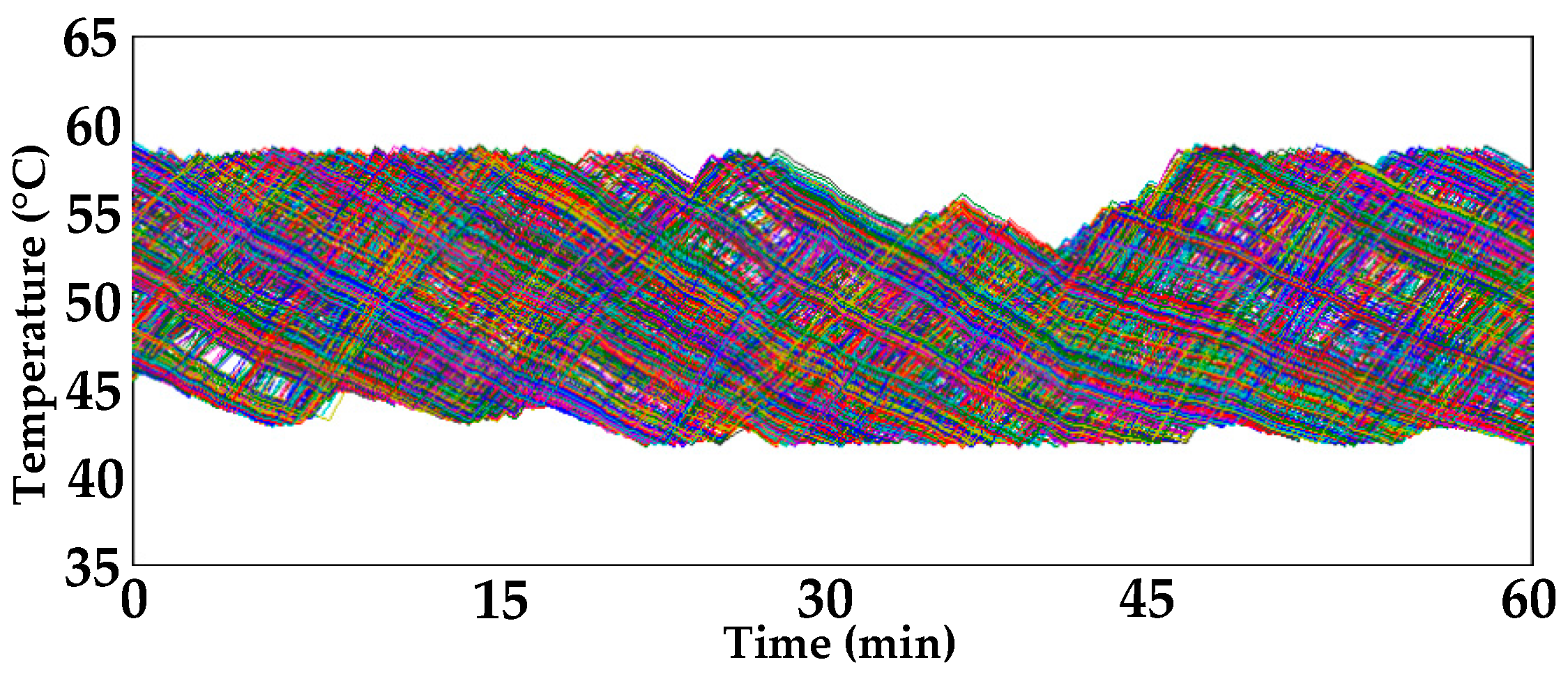
Figure 19 shows the results of the temperature trajectories of the EPP-WH with an average of 16 °C dead-band and 50 °C setpoint. Compared with Figure 1, it can be observed that a given number of water heaters have been controlled with some concaves left in the operating regions. As there is a unique correspondence between rising temperature and power consumption, the EPP-WH, which is integrated by TCAs, can produce good responses based on the targets sent from the control center.

5. Conclusions and Future Work

In this study, an efficient power plant was developed based on the thermostatic dynamic model of water heaters. A number of strategies, including load shedding calculation, top layer optimization, and improved TPL strategy with lock-on and off constraints, were proposed to establish the EPP-WH as a good candidate for frequency regulation. To evaluate the performance of the proposed method, case studies with different conditions were simulated under load control, and essential conclusions were drawn. The results showed that using the model and the proposed strategies, the EPP-WH had a good and stable frequency regulation performance. As a load-side solution, more types of TCAs, such as air-conditioners and heat pumps were recommended as frequency regulation resources. The optimization of lock-on and off time limits and price constraints will also be investigated in the future.