
Optimal Energy Scheduling and Transaction Mechanism for Multiple Microgrids


Department of Electronic Engineering, Sogang University, Seoul 04107, Korea
*
Author to whom correspondence should be addressed.
Energies 2017, 10(4), 566; https://doi.org/10.3390/en10040566
Submission received: 22 February 2017
/
Revised: 10 April 2017
/
Accepted: 18 April 2017
/
Published: 21 April 2017
(This article belongs to the Special Issue Smart Microgrids: Developing the Intelligent Power Grid of Tomorrow)
Abstract
:In this paper, we propose a framework for optimal energy scheduling combined with a transaction mechanism to enable multiple microgrids to exchange their energy surplus/deficit with others while the distributed networks of microgrids remain secure. Our framework is based on two layers: a distributed network layer and a market layer. In the distributed network layer, we first solve optimal power flow (OPF) using a predictor corrector proximal multiplier algorithm to optimally dispatch diesel generation considering renewable energy and power loss within a microgrid. Then, in the market layer, the agent of microgrid behaves either as a load agent or generator agent so that the auctioneer sets a reasonable transaction price for both agents by using the naive auction-inspired algorithm. Finally, energy surplus/deficit is traded among microgrids at a determined transaction price while the main grid balances the transaction. We implement the proposed mechanism in MATLAB (Matlab Release 15, The MathWorks Inc., Natick, MA, USA) using an optimization solver, CVX. In the case studies, we compare four scenarios depending on whether OPF and/or energy transaction is performed or not. Our results show that the joint consideration of OPF and energy transaction achieves as minimal a cost as the ideal case where all microgrids are combined into a single microgrid (or called grand-microgrid) and OPF is performed. We confirm that, even though microgrids are operated by private owners who are not collaborated, a transaction-based mechanism can mimic the optimal operation of a grand-microgrid in a scalable way.
1. Introduction
On 12 December 2015, in Paris, France, the 21st session of the Conference of the Parties (COP 21) to the United Nations Framework Convention on Climate Change (UNFCCC) adopted the Paris Agreement. Now, each country needs to achieve the submitted greenhouse gas (GHG) reduction targets and thus implements eco-friendly policies that encourage the use of eco-friendly energy such as renewable energy. Accordingly, conventional vertical energy industries based on fossil fuels are being gradually replaced by horizontal energy industries, and intensive studies on microgrids are ongoing these days. A microgrid is a power system that has distributed energy resources (DERs) to serve its internal load [1]. DERs include renewable energy such as photovoltaic (PV) and wind turbine (WT), distributed generators (DGs) and energy storage systems (ESSs) [2]. Microgrids are expected to maximize energy efficiency, be self-sufficient in electricity and thus be considered as one of the key technologies to resolve environmental problem concerns [3].
One of the most important problems in power systems is to supply high-quality power in a stable manner by matching supply and demand to sustain system reliability while minimizing operational cost. Note that it inevitably requires solving an optimal power flow (OPF) problem. However, acquiring a general solution of OPF for a large power system is very challenging because it is essentially a nonconvex optimization problem where some of equality constraints in the power balance equation are not affine. Previously, several algorithms such as mixed integer linear programming [4] and particle swarm optimization [5] were proposed but could not guarantee achieving optimality. Recently, the authors of [6,7,8] provided an optimal solution, which is computationally feasible and scalable, by relaxing the second order equality constraints into convex inequality constraints. They showed that the solution is exact, i.e., the solution is indeed on the boundary of the inequality constraints under some conditions [6,7].
Then, a series of their work focused on transmission networks [9] and also distribution networks [10]. However, careful consideration is required in applying the techniques into microgrids, which is the horizontal energy industry and thus there are more uncertainties from distributed, renewable generations and fluctuating loads. For example, PV generation may vary rapidly and load profile of small customers are less predictable or controllable [11]. Hence, to avoid additional difficulties in distribution networks, some of the existing works assume that all generators and loads are connected to one bus and ignore the associated power flow in distribution networks [12], i.e., just solving an economic dispatch problem. However, ignoring power flow in microgrids may lead to infeasible solutions in practice. In [13], the authors considered an energy management system (EMS) that performs load side management and schedules diesel generation as well as ESS charging/discharging. In doing this, they proposed a distributed optimization algorithm to effectively control local load and DG within a short time. Specifically, the distributed EMS consists of a microgrid controller and local controllers that jointly operate ESS, diesel generators and demand response in solving the OPF problem.
Besides power security issues, microgrids are being built in various facilities that need large power; complex buildings, hospitals, hotels, schools, unstable power supply areas, and military facilities require their own power sources [14]. With the proliferation of renewable generation and unbundling of the electrical power system industry, market-based energy management becomes more viable to meet their local objectives [15,16]. For example, transactive energy is introduced in New York state as an economic principle and control technique to manage the flow or exchange of energy. Consequently, one microgrid can sell its energy surplus to maximize its own profits by strategically bidding in a market. The other microgrid may also want to buy energy from another microgrid to minimize its operational cost by strategically bidding in the market. Designing a market mechanism for energy transaction among multiple microgrids is an active research area. For example, the work in [12] solved the problem by implementing an agent-based virtual market. They modeled energy transaction as a two-level problem. At an upper level, an auction agent (AA) solves a social welfare maximization problem, and at a lower level, microgrids try to minimize their operation costs. Thus, the upper level transaction problem is constrained by the lower level decision-agents. However, previous work assumed that all generators or loads in a microgrid are connected to a single bus and thus optimal power flow within the microgrid was not considered. In this regard, we investigate a transaction-enabled OPF problem to combine efficient energy transaction with optimal power flow. To the best of our knowledge, this is the first attempt to leverage energy transaction between microgrids considering OPF within a microgrid. Table 1 represents a comprehensive literature review that contrasts the previous approaches and the proposed one.
We summarize our key contributions as follows. We provide a framework for energy transaction combined with OPF. Each microgrid first solves its own OPF problem using a predictor corrector proximal multiplier (PCPM) algorithm and determines whether it is in the state of energy surplus or deficit, initially assuming that surplus/deficit energy can be balanced with the main grid/distribution system operator (DSO). In a market, a microgrid with energy surplus becomes a generator agent and a microgrid with energy deficit becomes a load agent. Then, energy transaction between microgrids is performed using the naive auction-inspired algorithm that indifferently determines the transaction price.
The agreed price incentivizes microgrids to exchange their energy with other microgrids so that distributed resources can be fully exploited. The virtue of employing the naive auction is that it maximizes the social benefits of all market participants. The proposed mechanism enables all microgrids to be better off by reducing operating cost within their own distributed network. To verify the transaction-enabled OPF algorithm, we compare four scenarios in case studies: (i) economic dispatch; (ii) OPF within microgrid; (iii) OPF combined with energy transaction; and (iv) finally all microgrids are assumed to be managed by a single owner, and thus OPF is solved across all microgrids, called grand-microgrid. Our results show that combining OPF with energy transaction, which is practical to preserve the privacy of each microgrid, achieves almost the same performance to the case of grand-microgrid; the gap of operational cost is only , which shows the effectiveness of the proposed mechanism.
The rest of the paper is constructed as follows. We present the system model in Section 2. In Section 3, we provide a framework to obtain optimal energy scheduling combined with negotiated transaction price. Then, we present the case studies with real topology of microgrids and evaluate the proposed mechanism in Section 4. Finally, we conclude the paper in Section 5.
2. System Model
We consider a system model for a multiple microgrids environment. In the proposed model, there are two layers as illustrated in Figure 1. The lower layer is a distributed network layer, which is responsible for energy management within each microgrid, and the upper layer is a market layer, which is designed to trade energy among microgrids. In Section 2.1, we first describe the distributed network layer, and in Section 2.2, we describe the market layer.
2.1. Distributed Network Layer Model for Energy Scheduling
We consider a microgrid energy management system (EMS) that has the objective of minimizing the operational cost of the microgrid while supplying reliable power. The distribution network layer is responsible for DG management within a microgrid. Note that there are two types of DG: dispatchable DG such as diesel generation and non-dispatchable DG such as renewable generation. To obtain optimum energy scheduling in the presence of the uncertain DG units, its prediction is crucial. The system model within a microgrid without considering transaction is based on the model of [13] as will be described shortly. Our model will be extended to the case of energy transaction across microgrids in Section 2.2. We assume that the prediction is reasonably accurate so we focus on the control of dispatchable DG in this paper. Indeed, the combination of two types of DGs is desirable to mitigate the uncertainties of non-dispatchable DG.
2.1.1. DG Model
A dispatchable DG unit such as diesel plays an important role in the power system connected with PV since it matches supply better than non-dispatchable PV. The cost function of diesel can be expressed in a linear form at each time as Equation (1):
where and are constants, and is a discrete time unit. The output power of diesel generator is constrained as follows:
where is the maximum generation. In order to consider the characteristics of the diesel generator, its maximum ramping rate is bounded by:
where is a ramping parameter, , and we have:
where , and denote active power, reactive power and apparent power of generator, respectively [6].
2.1.2. Distribution Network Model of a Microgrid
Consider a distribution network of a microgrid modeled by a connected graph , which is a tree topology for radial distribution systems where each node in represents a bus and each edge in represents a distribution line. Note that we use bus and node interchangeably and line and edge interchangeably. We denote a node by where and a line by . Bus 0 is usually used to denote a slack bus of which voltage is given, and power injection is variable. To emphasize that the slack bus of a microgrid is also responsible for energy transaction, we will denote the slack bus of the microgrid by e instead of 0 in the sequel. For each bus , let be the complex voltage and be the net complex power injection on bus i. For each line , let be the complex impedance on the line, be complex current from buses i to j and be the complex power flowing from buses i to j.
We assume that the complex voltage at the slack bus is given and the complex power injection is a variable. A set of generators and a set of loads connected to bus i are denoted by and , respectively. The net power at each bus i satisfies:
where , .
For power flow analysis of radial networks, voltages, currents and net powers satisfy the following three physical laws for all branches and all . Given , the variables where satisfy the Ohm’s law:
the power flow definition:
and power balance at each bus:
The following is referred to as the branch flow model (BFM) equations:
where and .
Equations (5)–(12) define a system with the variables , where will be used as optimization variables of OPF in Section 3. Delivering reliable and high-quality power is very important in the microgrids. However, the integration of DERs may increase the voltage significantly. In the microgrids, thus, we consider the following voltage tolerance constraint:
where and represents to the minimum and maximum voltage, respectively.
2.1.3. Net Power Model of a Microgrid
In the proposed EMS model, the microgrid is connected with the main grid. Hence, the microgrid is operated in a grid-connected mode. The microgrid can export/import power to/from the main grid in accordance with power surplus/deficit. If generated power is higher than load, the microgrid can sell its surplus power at a selling price. On the contrary, if load is higher than generated power, the microgrid can buy its deficit power at a buying price. Note that, throughout the paper, we use selling/buying terminology from the microgrid perspective, not the main grid. The cost function of trading is defined as follows:
where is trading power ( for importing and for exporting) and denotes transaction price, respectively. Note that this trading can be with the main grid or other microgrids. If this trading is with the main grid, is given by the time of use (TOU) of DSO. If this trading is with other microgrids, is determined at the market layer considering the bidding of all microgrids. The net power injected from the main grid to the microgrid is given by:
where e is the slack bus of the microgrid, and j is a bus connected to generators in the microgrid.
2.2. Market Layer Model for Energy Transaction
2.2.1. Three Agents in the Market Layer
The market layer of the proposed mechanism is responsible for maintaining fair market and power management among multiple microgrids. For this, we have load agent (LA), generator agent (GA) and an auction agent (AA). As noted above, the EMS of each microgrid determines whether to behave as LA or GA to minimize the cost of each microgrid. Then, as a market participant, the EMS discretizes the required export/import into energy units of equal size. Note that the minimum size of energy unit is arbitrary, and can be as small as possible unless it is a burden in the market layer. The details will be discussed in Section 3.2. The role of LA is to purchase energy units from the main grid or other microgrid. The role of GA is to sell energy units to the main grid or other microgrids. LA and GA submit this trading information reflecting supply–demand requirement to AA in the market. Upon receiving this information, AA runs an auction algorithm to determine transaction price as will be explained below.
2.2.2. The Naive Auction Mechanism
We introduce the naive auction mechanism, which is a well-known solution for the symmetric assignment problem [23]. The virtue of the naive auction is to maximize the total benefit of all market participants. Inspired by this mechanism, in Section 3.2, we will show that AA sets a reasonable transaction price for LA and GA so that microgrids can be better off. The general symmetric assignment problem is as follows. Suppose that there are X persons and Y objects that need to be matched on the one-to-one basis. It is called symmetric because . Then, there is benefit for matching a person with an object . The objective of the assignment problem is to find an assignment for all persons and all objects that maximizes the total benefit, i.e.,
In doing this, the persons compete for the objects. The price is associated with each object m and is updated by the bids of all persons during the auction. The actual value acquired by a person l allotted with an object m is the difference between the benefit and the price . Note that the actual value of a specific object m may be different depending on the person.
The bidding process for each person is to find an object that maximizes the value, e.g.,
Then, the person l updates a bid increment for the object m as follows:
where:
Note that and represent the best object value and the second best object value. Here, is required to avoid infinite iterations in case two or more objects provide the same maximum value to the same person. In each iteration, is updated by the maximum bidding for the object m, and the person who bids the highest acquires the object. When all objects are allotted, the auction ends.
3. Transaction-Enabled OPF in Microgrid Energy Management (EMS)
Now, we provide a general framework based on the distributed network layer, the market layer, and their interaction.
3.1. Solving OPF within an Individual Microgrid
To avoid unnecessary notational complexity, we do not use an additional notation to denote a specific microgrid, but the procedure in Section 3.1 should be done for all microgrids that want to participate in energy transaction.
EMS of the microgrid aims to minimize the cost of generation, the cost of energy transaction from the main grid/other microgrids, and power losses. EMS solves the following OPF problem at each time :
Problem: OPF
where , and are weighting parameters. EMS first considers the trading with DSO, so is initially given by TOU. We will see, however, that is updated in the market layer if energy transaction occurs at time . The OPF problem is nonconvex due to the quadratic equality constraint in Equation (12), and we relax the equality constraints to inequality constraints:
Then, EMS addresses the following convex relaxation problem,
Problem: OPF-r
In case the branch thermal limit constraint is required, one can explicitly add the following convex inequality constraint:
where is the branch thermal limit of branch [24]. Note that the problem of OPF-r in Equation (23) is still a convex optimization.
In order to solve the problem in a distributed way as a scalable solution that can incorporate many DGs, we use the PCPM algorithm. PCPM is an iterative algorithm, and DGs and EMS communicate to have an optimal scheduling. DG solves its optimal dispatch and EMS solves the power flow including power losses and energy transaction. The optimization of energy scheduling is to obtain DG output power and net power imported/exported to have the minimum cost. Let k be an iteration index. At , DGs set their initial schedules randomly and communicate them to EMS. and are the Lagrangian multipliers associated with the active and reactive power at bus i, respectively. At the kth iteration, EMS sends two control signals and to DGs where is a positive constant.
Then, each DG solves the following problem for each ,
Sub-Problem: DG
where and . The optimal and (which are the solution of Sub-Problem: DG) are set as and , respectively.
Then, EMS solves the following problem for each time ,
Sub-Problem: EMS
where and . The optimal and are set as and , respectively. At the end of the kth step, the generators communicate next schedules and to the EMS, and the EMS updates and for all . Set and repeat the process until convergence. When the difference between the optimal and the optimal converges to zero, the above algorithm converges to an optimal solution to OPF, and it determines the optimal energy scheduling for an individual microgrid.
3.2. Setting Transaction Price for Microgrids
Before microgrids exchange their surplus/deficit energy with each other, since individual microgrid is a price-taker of TOU from the main grid, its energy scheduling and operating cost highly depend on the buying and selling prices of TOU. Then, the key task of AA is to determine a reasonable price on which all selling/buying microgrids in the market layer can agree. For example, for those who have surplus energy, if a transaction price is set higher than the selling price of TOU, they are willing to sell to other microgrids rather than to the main grid, and thus microgrids can be better off at the corresponding price. Similarly, if a transaction price is lower than the buying price of TOU, microgrids with deficit energy can be incentivized by buying from other microgrids. In doing this, to determine their market positions, either a seller or a buyer, an individual microgrid first runs its EMS based on TOU and then reports its status of surplus/deficit energy to AA.
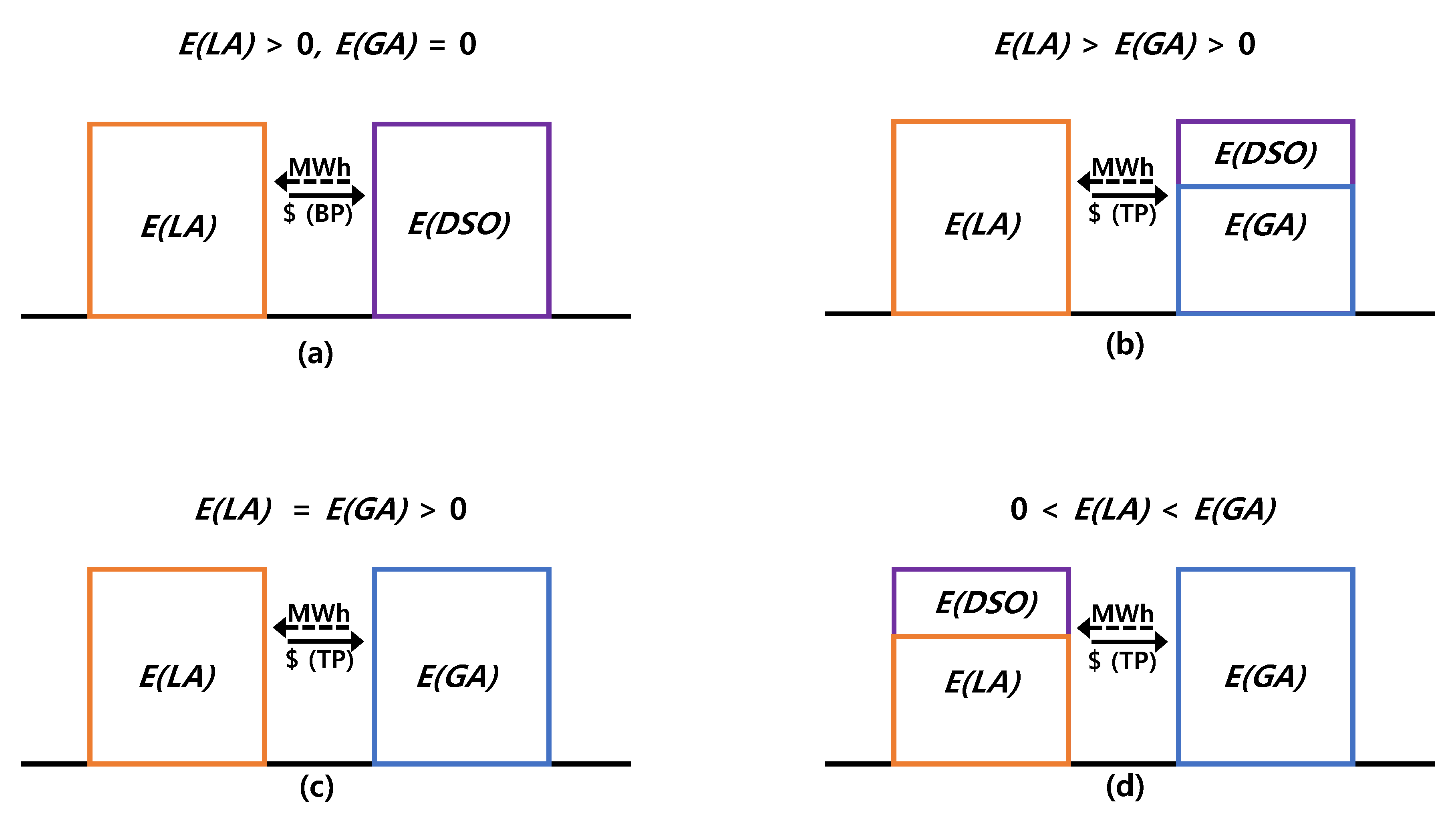
Once AA divides all microgrids into two groups of GA and LA, AA solves the symmetrical assignment problem based on the naive auction-inspired algorithm. Since the naive auction requires symmetric structure, i.e., the number of items and persons should be same [12,23]. Thus, the number of surplus energy units from GA and the number of deficit energy units from LA should be equal. If not, the main grid/DSO can fill the gap either as LA or GA according to the mismatch. For example, if the supply amount from GA is less than the demand amount from LA (see (a) and (b) in Figure 2), then AA allows DSO to supply the gap at TOU buying price, which is obviously much higher than the minimum selling price of GA. In (a) of Figure 2, a transaction price is simply the buying price with DSO because DSO only can provide LA with energy. In (b) of Figure 2, there are DSO and GA to supply LA with energy units. AA should guarantee the buying price with DSO as well as the marginal cost (or the initial selling price to DSO) of microgrids in GA. When the supply amount from GA is equal to the demand amount from LA (see (c) in Figure 2), any price between the buying and selling prices of TOU can reduce the total operating cost of microgrids. Finally, if the supply amount from GA is more than the demand amount from LA (see (d) in Figure 2), AA at least guarantees both the selling price with DSO and the marginal cost of microgrids. In this regard, AA sets a transaction price (TP) as follows:
where , denotes the energy of LA/GA, and BP, SP, and MC represent the buying and the selling prices with DSO, and marginal cost of microgrids in GA, respectively. Intuitively, as the surplus energy of GA increases, new transaction price decreases, which, in turn, implies that microgrids in LA can reduce operating cost by paying less than the buying price with DSO through energy transaction. By doing so, all microgrids are certainly incentivized and better off by accepting the energy transaction. It does not change the result of OPF as long as the marginal cost of DG is constant because, as long as the offered price by AA is higher than the marginal cost of DG, the GA would be fully utilized. Similarly, from an LA perspective, as long as the offered price by AA is lower than the buying price with DSO, the LA would be fully utilized. We summarize the procedure of interaction between solving OPF and setting prices in the Algorithm [TE-OPF]. In Section 4, we will demonstrate that the proposed combining approach successfully achieves operating cost reduction based on OPF and energy transaction.
| Algorithm [TE-OPF]: Transaction-enabled optimal power flow |
| Solving OPF within an individual microgrid (distributed network layer) |
| Require: The AA announces the initial buying and selling prices (TOU) to microgrids. Input: , and (randomly initialized).
|
| Setting prices for energy trading (market layer) |
Require: AA determines the status of microgrids, e.g., either GA or LA.
|
4. Case Studies
So far, we have described the two-layer mechanism that involves both energy transaction and OPF. In this section, we present case studies based on the realistic topology of microgrids and system parameters, and then evaluate performances of different scenarios.
Figure 3a shows that two microgrids are connected to the main grid to reliably balance their own load and power generation. For example, microgrid 1 consists of a diesel generator, load, and PV, and microgrid 2 has a diesel generator, load, and WT. The marginal cost of diesel generators for microgrid 1 and microgrid 2 are $80 and $100, respectively. In our simulations, the time step is one hour, and we operate microgrids during the day, e.g., . The maximum power of microgrid 1 and microgrid 2 are set to 4 MW and 1 MW, respectively. The ramping parameter is chosen to be 0.3 for all diesel generators in the microgrids. To be realistic, we use the DSO’s electricity tariff from the Korea Electric Power Corporation (KEPCO), which reflects a TOU electricity pricing model [25]. Microgrids can buy/sell their deficit/surplus energy directly from/to the main grid, and the buying and selling prices are shown in Figure 3b. Figure 3c shows detailed renewable generation information.
It should be noted that our paper focuses on stationary analysis on optimal power flow within each microgrid and energy transaction among microgrids. For real operation, extreme scenarios and transient behaviors need to also be considered such as renewable energy outage or diesel generations in maintenance stage, etc., which are beyond the scope of this paper.
Based on power system parameters, we have four case studies as follows. Although microgrids solve economic dispatch by trading power with the main grid (Case 1), economic dispatch, per se, may result in electric overloads or inadequate voltage levels at local buses because it ignores the distribution line limits. In this regard, we solve an OPF of the microgrid to reduce unnecessarily high operating costs by optimizing the generation, while the distribution networks are considered to combine economic dispatch with power flow (Case 2). Note that Case 1 and Case 2 serve as two baselines, which correspond to the previous methods; Case 1 is the simplest one (economic dispatch) and Case 2 only considers OPF within a microgrid. Furthermore, Case 4 provides the minimum operational cost, which will be compared with our proposed algorithm. The transaction-enabled OPF algorithm enables the microgrids to exchange their local power with each other instead of trading power only with the main grid, especially when the microgrids can achieve cost-efficient and privacy-preserving operation (Case 3). Finally, the distributed scheme in Case 3 will be compared with a centralized energy system management (Case 4) in terms of system operating costs where two microgrids are assumed to be merged and collectively controlled.
4.1. Case 1: Without OPF nor Energy Transaction in Microgrids
In this baseline case, since microgrids cannot exchange their local energy with each other, TOU of DSO plays a main role in operating microgrids. In addition, considering only economic dispatch may possibly cause less economic or unreliable power system operation. Figure 4 shows 24 h energy scheduling when the microgrids are connected to the main grid. As can be seen, both microgrids have similar load patterns during the day. Note, however, that the generations of two microgrids are economically dispatched in different ways because it depends on TOU as well as different marginal cost and different renewable generation. Microgrid 1 is with PV and microgrid 2 is with WT, and their active generation times are also different: during a day vs. a night. Table 2 represents the operating costs for both microgrids. Next, we solve OPF to microgrids and evaluate the performance in terms of operating cost.
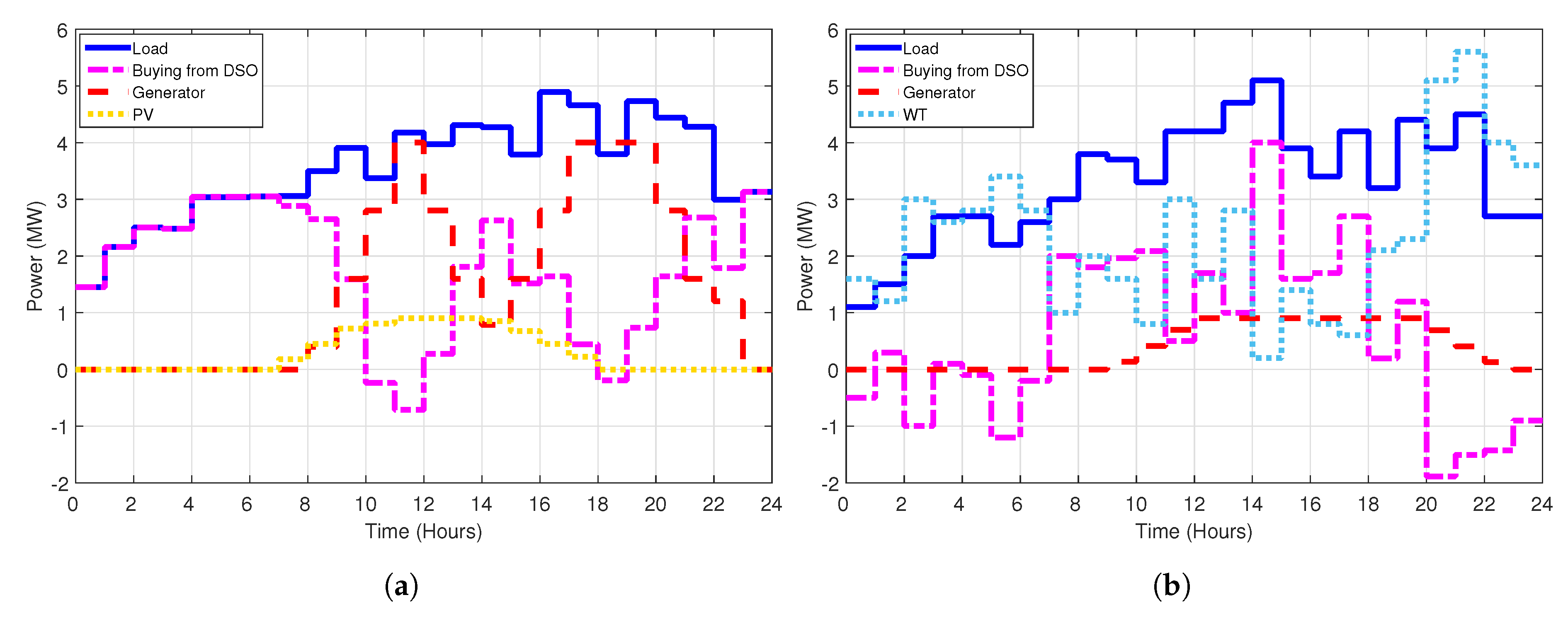
4.2. Case 2: Optimal Power Flow within Microgrids without Energy Transaction
In this case, microgrids consider the topological and electrical characteristics of power grid networks. Since energy transaction is not yet reflected between the microgrids, optimal energy scheduling is determined based on TOU of DSO. To consider the characteristics of a power distribution system, the voltage tolerance is set to be [0.95 p.u., 1.05 p.u.]. The parameters related to DG and power flow are chosen as , and . Figure 5 represents 24 h optimal energy scheduling based on the characteristics of the topology in Figure 3a. Microgrids utilize TOU of DSO and operate their internal network more efficiently and reliably, compared with Case 1. When the marginal cost of DG is more expensive than the buying price from DSO, the microgrid is willing to buy energy from DSO. When the microgrid has surplus renewable energy or the selling price of TOU is high, it optimizes power scheduling to minimize operating cost. Table 3 shows the operating cost of both microgrids. Compared with the baseline case, both microgrids reduce operating cost by $323.7 and $61.4, respectively, and total cost savings is $385.1. Next, we apply the transaction-enabled OPF algorithm to microgrids so that total cost can be reduced under a reliable system operation.
4.3. Case 3: Optimal Power Flow with Energy Transaction in Microgrids
Energy transaction between microgrids could lead to a considerable reduction of dispatch cost. In this case, we expect the synergy effect, which is achieved by combining OPF and energy transaction on microgrids. Given surplus/deficit generation in microgrids, we investigate energy transaction price between microgrids based on the naive auction-inspired algorithm. Figure 6 shows that the transaction prices incentivize microgrids to exchange their energy with each other instead of trading with the main grid/DSO. We notice that energy transaction between two microgrids occurs for 12 time slots during one day. For those slots that have no transaction record, we simply assign zero-prices for plotting purposes. Based on these transaction prices, the optimal energy scheduling for both microgrids is presented in Figure 7. Compared with Case 1 and Case 2, we can achieve further improvement of optimal energy scheduling for Case 3. This is possible because we not only consider diesel characteristics and voltage tolerance in the distributed network of microgrids, but also introduce a transaction process to reduce total operation cost. In the practical power system, Case 3 enables local microgrids to preserve their privacy information while securing power networks to avoid the voltage step change, which occurs on the sudden disconnection of a distributed generation or instantaneous over-current. Table 4 represents 24 h operating cost, which is certainly reduced compared with the previous cases.
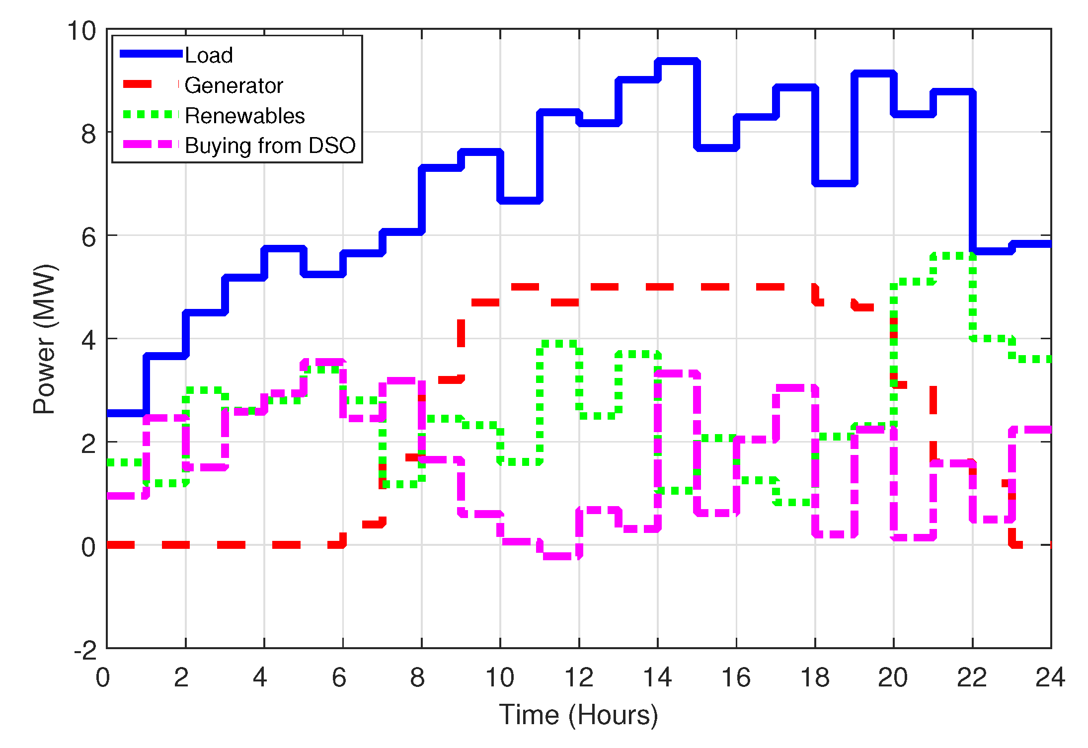
4.4. Case 4: Centralized Optimal Power Flow for All Microgrids
Suppose that an authorized entity has all information of components in microgrids to optimally balance load and generation while the distribution system is secured to combine economic dispatch with reliable power flow. Under the centralized OPF approach, Figure 8 shows 24 h optimal power scheduling, and Table 5 summarizes all the cases in terms of OPF, energy transaction, and total operating cost. Since the authorized entity does not necessarily need an additional transaction process, it can use information of marginal costs of microgrids as well as TOU of DSO. We notice that, although the centralized OPF is the ideal case, the proposed algorithm of Case 3 shows very close performance in terms of total operating cost, i.e., the gap is only 0.063%, which demonstrates the virtue of the proposed two-layer approach, i.e., transaction-based OPF operation.
5. Conclusions
In this paper, we proposed a novel framework for multiple microgrids, which is based on solving optimal power flow within a microgrid and energy transaction across microgrids. In doing this, we have used the PCPM algorithm for OPF and have proposed a naive auction-inspired algorithm for energy transaction. The transaction price is determined indifferently so that both microgrids can agree on the transaction price following the concept of the naive auction. To be realistic, we used a real topology of microgrids that have diesel generators, loads, and renewable generations such as solar and wind while considering TOU data from DSO. The transaction-enabled the OPF algorithm successfully reduced total operating cost while the distributed networks of microgrids remain secured. To validate the proposed approach, we compare the following cases: whether OPF is considered or not, whether energy transaction is considered or not, and, finally, all microgrids are combined into a single one (grand-microgrid). Our results showed that energy transaction based on the proposed transaction price successfully reduces the operational costs of both microgrids. Furthermore, the combined approach of OPF within a microgrid and energy transaction across microgrids achieve near-optimal performance compared to the case of the grand-microgrid; the performance gap is only 0.063%. This result is promising because while preserving the privacy of each microgrid, the total cost of microgrids can be kept as low as the ideal case. Our future work includes how to quantify the contribution of DSO in energy transaction and derive an appropriate transaction fee paid to DSO in order to acknowledge its role in balancing distribution networks.
Acknowledgments
This research was supported by the Korea Electric Power Corporation (KEPCO) (CX72166553-R16DA17) of the Republic of Korea.
Author Contributions
The paper was prepared by a collaborative effort of the authors. Boram Kim designed the algorithm, performed the simulations, and collectively prepared the manuscript. Sunghwan Bae designed the case study scenarios. Hongseok Kim led the project and research. All authors discussed the results and approved the publication.
Conflicts of Interest
The authors declare no conflict of interest.
References
- Kim, H.; Thottan, M. A two-stage market model for microgrid power transactions via aggregators. Bell Labs Tech. J. 2011, 16, 101–107. [Google Scholar] [CrossRef]
- Choi, Y.; Kim, H. Optimal scheduling of energy storage system for self-sustainable base station operation considering battery wear-out cost. Energies 2016, 9, 462. [Google Scholar] [CrossRef]
- Lasseter, R.H.; Paigi, P. Microgrid: A conceptual solution. In Proceedings of the IEEE 35th Annual Power Electronics Specialists Conference, Aachen, Germany, 20–25 June 2004; pp. 4285–4290. [Google Scholar]
- Morais, H.; Kadar, P.; Faria, P.; Vale, Z.A.; Khodr, H. Optimal scheduling of a renewable micro-grid in an isolated load area using mixed-integer linear programming. Renew. Energy 2010, 35, 151–156. [Google Scholar] [CrossRef]
- Abido, M. Optimal power flow using particle swarm optimization. Int. J. Electr. Power Energy Syst. 2002, 24, 563–571. [Google Scholar] [CrossRef]
- Low, S.H. Convex relaxation of optimal power flow, Part I: Formulations and equivalence. IEEE Trans. Control Netw. Syst. 2014, 1, 15–27. [Google Scholar] [CrossRef]
- Low, S.H. Convex relaxation of optimal power flow, part II: Exactness. IEEE Trans. Control Netw. Syst. 2014, 1, 177–189. [Google Scholar] [CrossRef]
- Lavaei, J.; Low, S.H. Zero duality gap in optimal power flow problem. IEEE Trans. Power Syst. 2012, 27, 92–107. [Google Scholar] [CrossRef]
- Madani, R.; Sojoudi, S.; Lavaei, J. Convex relaxation for optimal power flow problem: Mesh networks. IEEE Trans. Power Syst. 2015, 30, 199–211. [Google Scholar] [CrossRef]
- Gan, L.; Li, N.; Topcu, U.; Low, S.H. Exact convex relaxation of optimal power flow in radial networks. IEEE Trans. Autom. Control 2015, 60, 72–87. [Google Scholar] [CrossRef]
- Ryu, S.; Noh, J.; Kim, H. Deep neural network based demand side short term load forecasting. Energies 2016, 10, 3. [Google Scholar] [CrossRef]
- Nunna, H.K.; Doolla, S. Multiagent-based distributed-energy-resource management for intelligent microgrids. IEEE Trans. Ind. Electron. 2013, 60, 1678–1687. [Google Scholar] [CrossRef]
- Shi, W.; Xie, X.; Chu, C.C.; Gadh, R. Distributed optimal energy management in microgrids. IEEE Trans. Smart Grid 2015, 6, 1137–1146. [Google Scholar] [CrossRef]
- Ersal, T.; Ahn, C.; Hiskens, I.A.; Peng, H.; Stein, J.L. Impact of controlled plug-in EVs on microgrids: A military microgrid example. In Proceedings of the 2011 IEEE Power and Energy Society General Meeting, Detroit, MI, USA, 24–29 July 2011; pp. 1–7. [Google Scholar]
- Dimeas, A.L.; Hatziargyriou, N.D. Operation of a multiagent system for microgrid control. IEEE Trans. Power Syst. 2005, 20, 1447–1455. [Google Scholar] [CrossRef]
- Logenthiran, T.; Srinivasan, D.; Khambadkone, A.M. Multi-agent system for energy resource scheduling of integrated microgrids in a distributed system. Electr. Power Syst. Res. 2011, 81, 138–148. [Google Scholar] [CrossRef]
- Paschalidis, I.C.; Li, B.; Caramanis, M.C. Demand-side management for regulation service provisioning through internal pricing. IEEE Trans. Power Syst. 2012, 27, 1531–1539. [Google Scholar] [CrossRef]
- Lee, S.; Jin, Y.; Jang, G.; Yoon, Y. Optimal bidding of a microgrid based on probabilistic analysis of island operation. Energies 2016, 9, 814. [Google Scholar] [CrossRef]
- Liu, G.; Xu, Y.; Tomsovic, K. Bidding strategy for microgrid in day-ahead market based on hybrid stochastic/robust optimization. IEEE Trans. Smart Grid 2016, 7, 227–237. [Google Scholar] [CrossRef]
- Maity, I.; Rao, S. Simulation and pricing mechanism analysis of a solar-powered electrical microgrid. IEEE Syst. J. 2010, 4, 275–284. [Google Scholar] [CrossRef]
- Song, N.O.; Lee, J.H.; Kim, H.M. Optimal electric and heat energy management of multi-microgrids with sequentially-coordinated operations. Energies 2016, 9, 473. [Google Scholar] [CrossRef]
- Hussain, A.; Bui, V.H.; Kim, H.M. Robust optimization-based scheduling of multi-microgrids considering uncertainties. Energies 2016, 9, 278. [Google Scholar] [CrossRef]
- Bertsekas, D.P. Auction algorithms for network flow problems: A tutorial introduction. Comput. Optim. Appl. 1992, 1, 7–66. [Google Scholar] [CrossRef]
- Vovos, P.N.; Bialek, J.W. Direct incorporation of fault level constraints in optimal power flow as a tool for network capacity analysis. IEEE Trans. Power Syst. 2005, 20, 2125–2134. [Google Scholar] [CrossRef]
- Korea Electric Power Corporation (KEPCO). Available online: http://cyber.kepco.co.kr/ckepco/front/jsp/CY/E/E/CYEEHP00103.jsp (accessed on 20 April 2017).
Figure 1.
The overall structure of multiple microgrids. PCPM: predictor corrector proximal multiplier; TOU: time of use; and DSO: distribution system operator.
Figure 1.
The overall structure of multiple microgrids. PCPM: predictor corrector proximal multiplier; TOU: time of use; and DSO: distribution system operator.
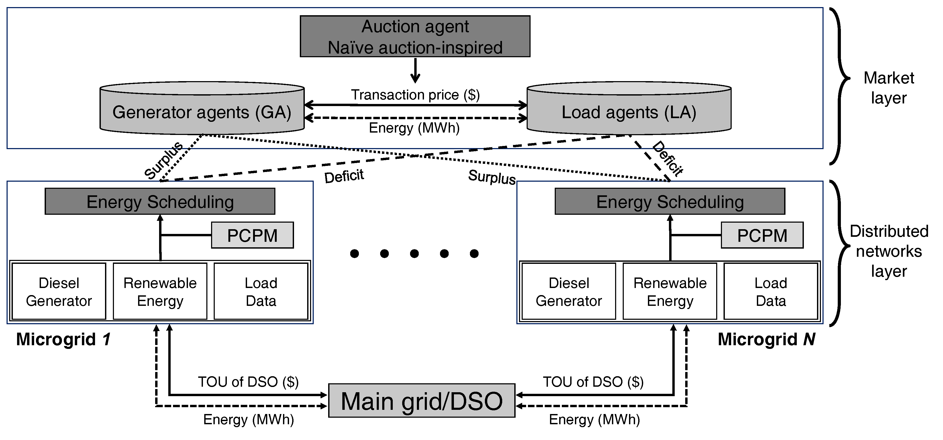
Figure 2.
Examples of balancing scenarios by auction agent. ( denotes the amount of energy of either LA, GA or DSO.)
Figure 2.
Examples of balancing scenarios by auction agent. ( denotes the amount of energy of either LA, GA or DSO.)

Figure 3.
(a) The topology of microgrids; (b) transaction price from the main grid; and (c) renewable energy profile.
Figure 3.
(a) The topology of microgrids; (b) transaction price from the main grid; and (c) renewable energy profile.
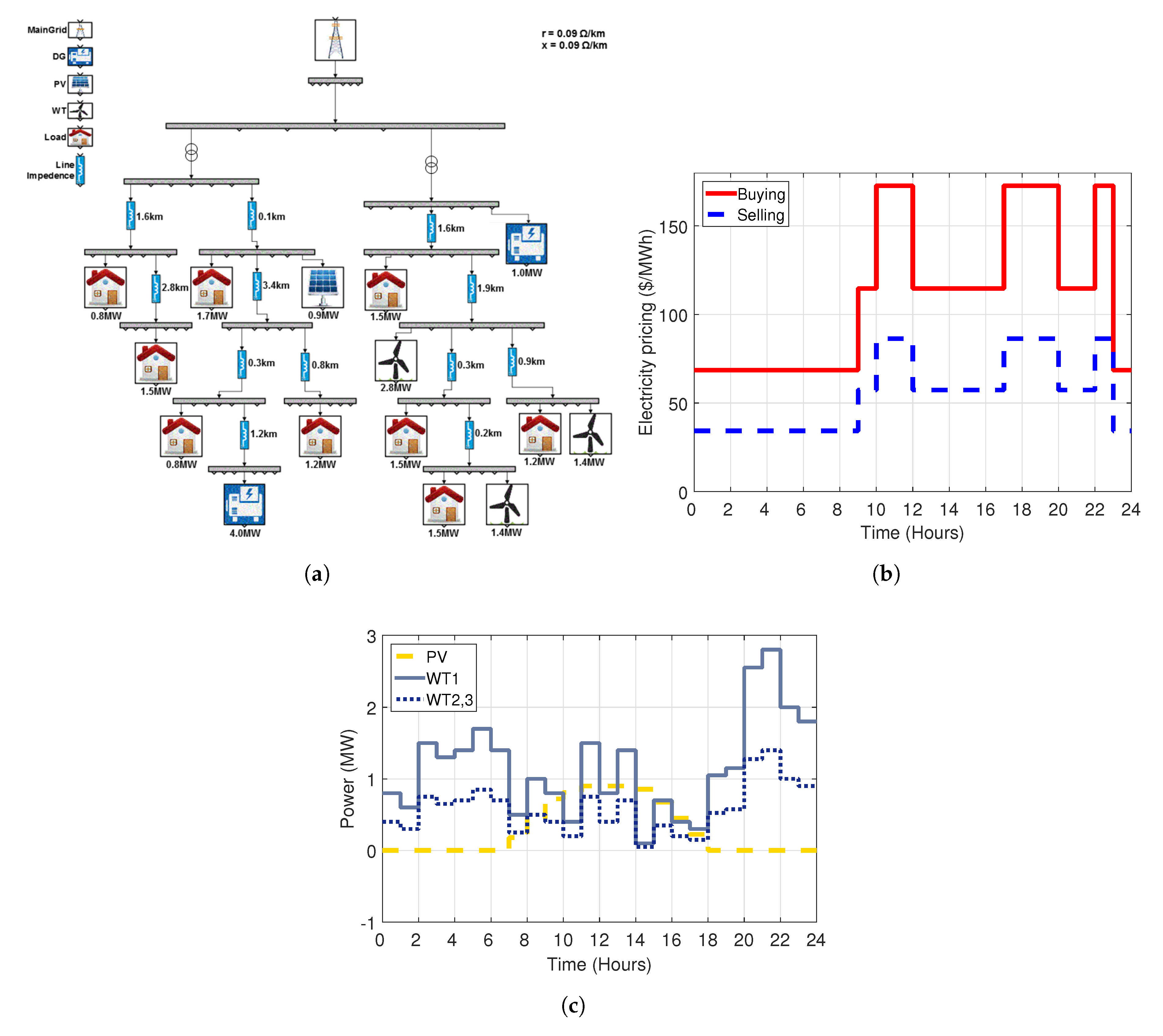
Figure 4.
Case 1: load profile and power scheduling based on non-OPF operation. (a) Microgrid 1; and (b) microgrid 2. OPF: optimal power flow.
Figure 4.
Case 1: load profile and power scheduling based on non-OPF operation. (a) Microgrid 1; and (b) microgrid 2. OPF: optimal power flow.
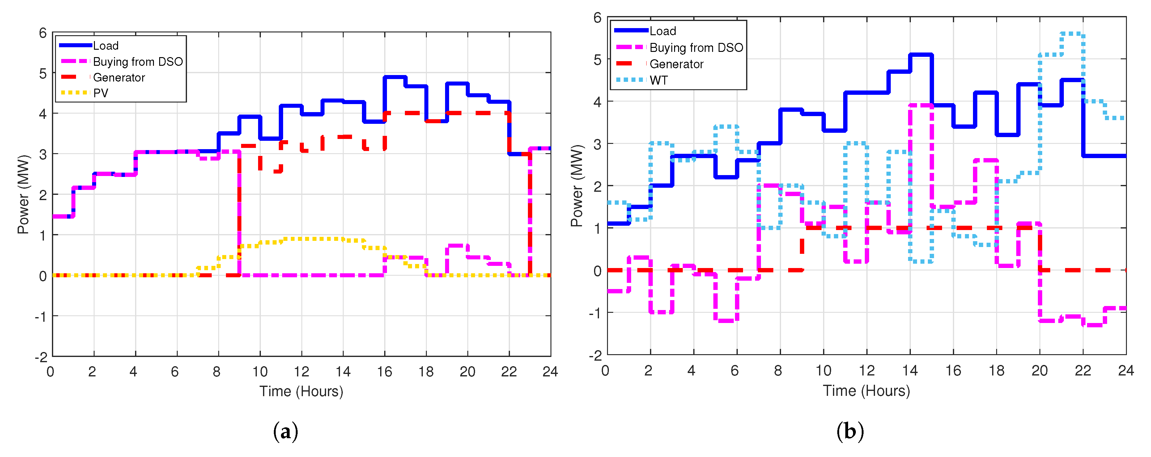
Figure 5.
Load profile and power scheduling based on OPF operation: (a) microgrid 1; and (b) microgrid 2.
Figure 5.
Load profile and power scheduling based on OPF operation: (a) microgrid 1; and (b) microgrid 2.

Figure 6.
Energy transaction price between microgrids.
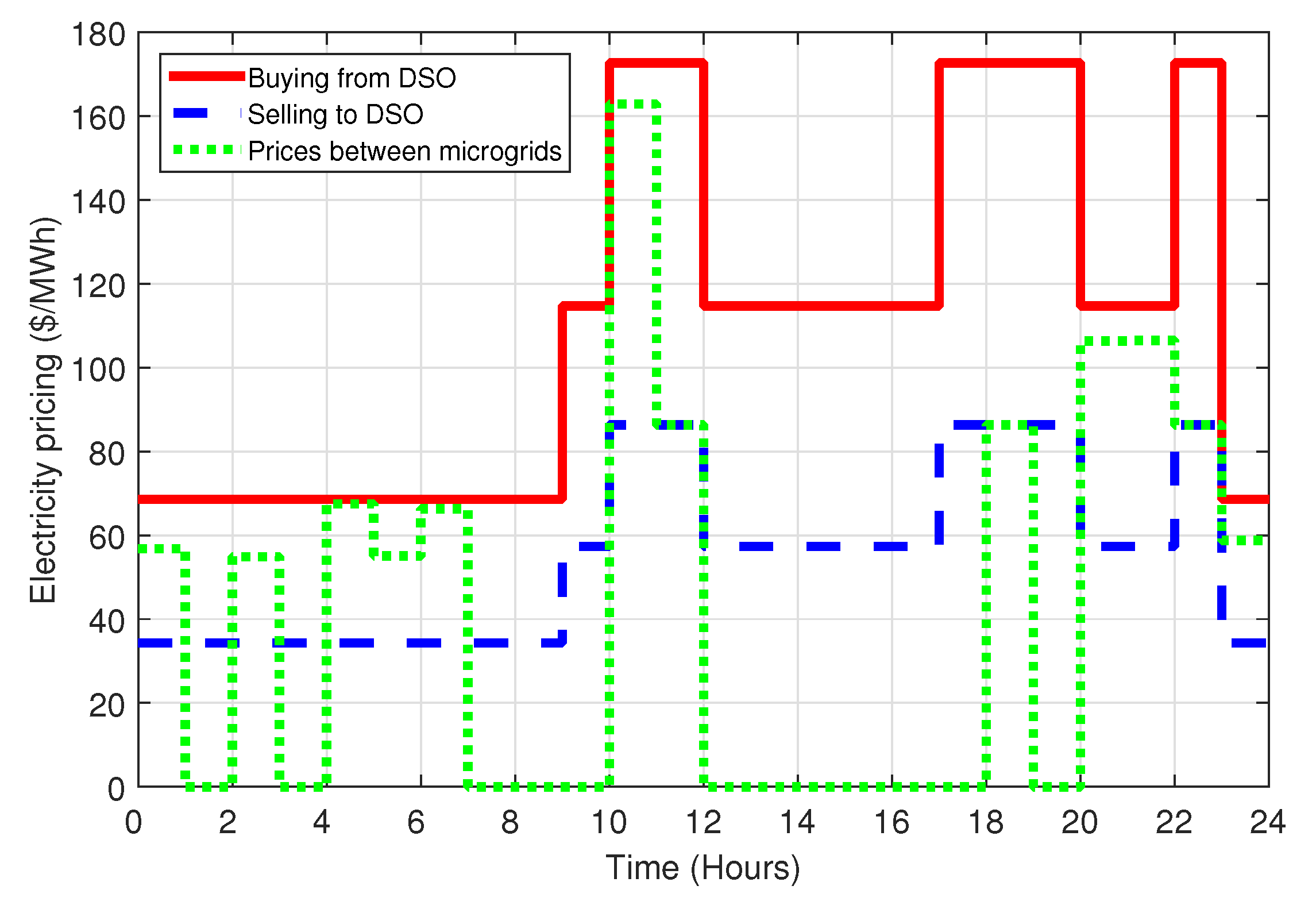
Figure 7.
Case 3: load profile and power scheduling based on the transaction-enabled OPF algorithm. (a) Microgrid 1; and (b) microgrid 2.
Figure 7.
Case 3: load profile and power scheduling based on the transaction-enabled OPF algorithm. (a) Microgrid 1; and (b) microgrid 2.
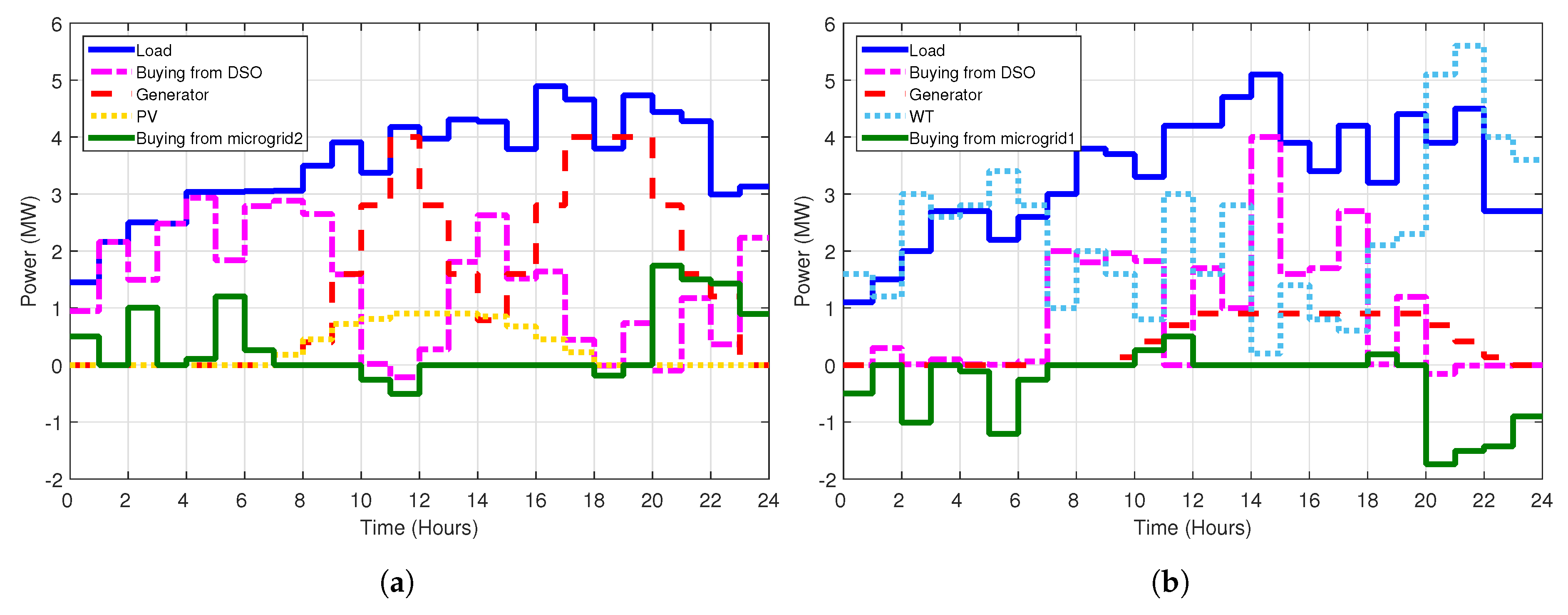
Figure 8.
Load profile and power scheduling based on the centralized optimal power flow.


Table 1.
Summary of optimal power flow and energy transaction algorithm in literature.
| References | Algorithm for Solving Optimal Power Flow |
| (This Paper) | Predictor corrector proximal multiplier |
| [4] | Mixed-integer linear programming |
| [5] | Particle swarm optimization |
| [6,7] | Uadratic program, semidefinite programming, second-order cone programming |
| [8] | Semidefinite programming, polynomial-time algorithm |
| [9] | Semidefinite programming relaxation |
| [10] | Second-order cone programming relaxation |
| References | Algorithm for Solving Energy Transaction |
| (This Paper) | Naive auction-inspired algorithm |
| [17] | Stochastic modeling, stochastic dynamic programming |
| [18] | Pattern search algorithm |
| [19] | Hybrid stochastic, robust optimization |
| [20] | Auction theory, weighted majority algorithmm |
| [21] | Sequentially coordinated operation |
| [22] | Robust optimization |
Table 2.
24 hour operating cost in Case 1.
| Microgrid 1 | Microgrid 2 | Total Cost | |
|---|---|---|---|
| Operating cost ($) |
Table 3.
24 h operating cost in Case 2.
| Microgrid 1 | Microgrid 2 | Total Cost | |
|---|---|---|---|
| Operating cost ($) |
Table 4.
24 h operating cost in Case 3.
| Microgrid 1 | Microgrid 2 | Total Cost | |
|---|---|---|---|
| Operating cost ($) |
Table 5.
Summary of all cases.
| Microgrid with OPF | Microgrid with Energy Transaction | Total Operating Cost ($) | |
|---|---|---|---|
| Case 1 | X | X | |
| Case 2 | O | X | |
| Case 3 | O | O | |
| Case 4 | - | - |
© 2017 by the authors. Licensee MDPI, Basel, Switzerland. This article is an open access article distributed under the terms and conditions of the Creative Commons Attribution (CC BY) license (http://creativecommons.org/licenses/by/4.0/).
Share and Cite
MDPI and ACS Style
Kim, B.; Bae, S.; Kim, H. Optimal Energy Scheduling and Transaction Mechanism for Multiple Microgrids. Energies 2017, 10, 566. https://doi.org/10.3390/en10040566
AMA Style
Kim B, Bae S, Kim H. Optimal Energy Scheduling and Transaction Mechanism for Multiple Microgrids. Energies. 2017; 10(4):566. https://doi.org/10.3390/en10040566
Chicago/Turabian StyleKim, Boram, Sunghwan Bae, and Hongseok Kim. 2017. "Optimal Energy Scheduling and Transaction Mechanism for Multiple Microgrids" Energies 10, no. 4: 566. https://doi.org/10.3390/en10040566
Note that from the first issue of 2016, this journal uses article numbers instead of page numbers. See further details here.