
Development of Novel Robust Regulator for Maximum Wind Energy Extraction Based upon Perturbation and Observation


School of Electric Power Engineering, South China University of Technology, Guangzhou 510640, China
*
Author to whom correspondence should be addressed.
Energies 2017, 10(4), 569; https://doi.org/10.3390/en10040569
Submission received: 6 January 2017
/
Revised: 31 March 2017
/
Accepted: 13 April 2017
/
Published: 21 April 2017
Abstract
:This paper develops a robust regulator design approach to maximum power point tracking (MPPT) of a variable-speed wind energy conversion system (WECS) under the concept of perturbation and observation. The proposed perturb and observe regulators (PORs) rooted on the sliding mode method employs the optimal power curve (OPC) to realize MPPT operations by continuously adjusting rotor speeds and the duty cycles, which can ensure control performance against system parameter variations. The proposed PORs can detect sudden wind speed changes indirectly through the mechanical power coefficient, which is used to acquire the rotor speed reference by comparing it with the optimal power constant. For the speed and duty cycle regulation, two novel controllers based on the proposed POR, i.e., an MPPT controller and a speed controller, are devised in this research. Moreover, by applying the small-signal analysis on a nonlinear wind turbine system, the convergence of the proposed speed controller is proven for the first time based on the Lyapunov theory, and meanwhile, a single-pole transfer function, to describe the effect of duty cycle variations on rotor speeds, is designed to ensure its stability. The proposed strategy is verified by simulation cases operated in MATLAB/Simulink and experimental results performed from a 0.5-kW wind turbine generator simulator.
1. Introduction
Wind energy conversion systems (WECSs) are widely used to convert wind energy into different forms of electrical energy through a wind turbine and a power conversion system [1]. To operate a WECS at an optimum power extraction point, the maximum power point tracking (MPPT) in variable-speed operation systems attracts much attention [2]. Generally, the current MPPT methods can be classified into three major types: power signal feedback (PSF) control, tip speed ratio (TSR) control and hill climbing searching (HCS) control.
A PSF method, designed based on a maximum power curve of a wind turbine, needs rotor speeds for yielding a power reference [3,4]. The optimal reference power curve is programmed in a microcontroller memory, working as a lookup table [2]. Due to the tracking speed being dependent on the rotor inertia of a wind turbine, a larger rotor inertia may lead to a slow tracking speed especially in low wind speed conditions [5]. Kim and Van adopted a proportional control loop to improve the fast performance of the MPPT control [6].
In TSR control, anemometers are usually required to measure wind speeds [7,8]. Although this method is simple in implementation, its performance highly depends on the reliability of anemometers, which is a challenge for such methods. Wind speed estimation methods were proposed to solve such a problem [9]. Using complex estimation algorithms, wind speeds can be captured with respect to the optimal tip speed radio, so that MPPT can be implemented.
Most practised wind energy control systems are based on the HCS algorithm due to its simplicity in hardware and software, which does not require any previous knowledge of the wind turbine and generator [4,10]. The idea of the method is the online measurement of the output power and observing the change rate of power with respect to speed, i.e., , to extract maximum power from a WECS [11]. MPPT is achieved when , through adjusting either the rotor speed or duty cycle of a converter [12]. This method relies on a large amount of online computation, and thus, it is difficult to achieve MPPT for fast-varying wind speeds, which considerably decreases its dynamic performance. In [4,10], an adaptive step size was adapted to keep up with rapid wind speed changes through a peak detection method under changing wind conditions. In [11,12], a constant step size was replaced by the rate of power change with respect to perturbing variables, e.g., the rotor speed. In [13], an improved hill climb searching (IHCS) was proposed to realize MPPT operations. The advantage of the method is that it can immediately search the optimal operating point, thereby reducing the searching procedure time. However, the performance of the method depends on the anemometer accuracy. Alternatively, an estimated wind speed can be utilized for this method [9].
In WECSs, the electrical and mechanical parts behave as a nonlinear system [14], where electromechanical parameter variations are a well-recognized problem [15]. To overcome this problem, different nonlinear control techniques were accepted, such as fuzzy logic control [4], fractional order control [7] and adaptive control [9]. Among robust control techniques, the sliding mode control (SM) methods [15,16] made plants more robust, invariant with respect to matched uncertainties, which were computationally simple with respect to other robust control approaches. In order to enhance the transient tracking capability of a traditional HCS algorithm in the presence of rapidly-changing wind speeds and model uncertainty, a perturb and observe regulator (POR) is first proposed in this research. Two novel controllers, e.g., the POR-based MPPT controller and speed controller, are proposed to estimate a rotor speed reference and an optimal duty cycle, respectively.
In [11], a traditional HCS algorithm required measurements of the output power and checking in real time, which was difficult to track the reference signal at fast-varying wind speeds. To overcome this problem, an optimal power coefficient (OPC) curve is for the first time proposed, which includes a fixed optimal power coefficient fitted for all of the wind speeds and the rotor speeds. For the sake of the proposed OPC curve, the control system has been integrated, from one side, with the proposed POR-based MPPT controller, so as to improve the efficiency and energy extraction just by tracking the OPC at all of the winds; from the other side, with techniques for estimating the mechanical power coefficient and reducing current sensors. Particularly, no current loop is used in the proposed MPPT control strategy because of the merits of the proposed PORs.
The rest of this paper is organized as follows: Section 2 presents the modelling of a WECS. An adaptive MPPT strategy is then developed in Section 3. Section 4 presents how to design the proposed PORs and analyse the stability of them based on the Lyapunov theory and the small-signal analysis. Simulation and experimental verifications are presented and discussed in Section 5 and Section 6, respectively. The conclusion is in Section 7.
2. Modelling of WECS and Linearization Analysis
The schematic from the studied system is shown in Figure 1. Through a diode rectifier, the output power from a permanent magnet synchronous generator (PMSG) is transferred to a speed-controlled DC/DC converter, which is used to control the speed of the studied WECS. In this research, the studied system adopts a resistor as the load representing a DC system, and the maximum power point (MPP) is reflected across the resistor [10,17].
The control block diagram of the proposed MPPT strategy presented in Figure 1 is composed of three parts, where Block A is the estimator for calculating defined as the mechanical power coefficient [4], Block B is the POR-based MPPT controller used to track the optimal power constant and Block C is the POR-based speed controller applied to track the estimated rotor speed reference .
2.1. Modelling of Wind Turbine and PMSG
The input mechanical power of wind turbine, , is given by [18]:
In this research, an approximate polynomial is used to represent the function, and it is illustrated by Equation (2) [19], which is a nonlinear expression of as a function of for the studied WECS.
= 0.304 is achieved at = 6.29 and = [20].
Furthermore, the wind turbine parameters, e.g., , , can be acquired by calculating the coordinate of extreme point in the function of (3). To clearly present the main idea of the research, is assumed to be a constant value, e.g., 1.205 at the temperature of 20 C. Nevertheless, the impact of temperature variations on is also discussed at the end of Case 3 in Section 5.
The dynamic voltage equations of a surface-mounted PMSG are represented in the rotational reference frame (d-q) as follows [7]:
The electrical parameters of a PMSG in Appendix A, i.e., the stator resistance per phase, the stator inductance per phase and the rotor PM flux linkage, are measured using standard tests, i.e., an open-circuit test, a blocked-rotor test and a load test [21].
2.2. Linearization Analysis of WECS
The mechanical torque with one-mass modelling of WECS and the generator torque are expressed as below [4,6]:
For the small-signal analysis, applying a small perturbation at the operating point () of the mechanical torque and generator torque in (6) and (7), respectively:
Based on (6) to (9), the mechanical torque and generator torque are rewritten applying the Laplace transform as:
The duty cycle to the DC-DC boost converter is expressed as [22]:
As reported in [10], the rotor speed cannot be changed instantly as it is limited by the system inertia. In [4], taking into account that is proportional to for PMSG,
According to the proposed analysis, is changed instantly while the DC-link voltage associated with in (13) is changed slowly, and can be regarded as a constant value . Based on this analysis, can be expressed with the corresponding d in a sampling period of switch according to (12):
where .
For the small-signal analysis, at an operating point can be linearized by Taylor series, which is expressed as:
where is the duty cycle at the operating point.
Based on (15), it is deduced that:
It shows that is linearly proportional to around an operating point. Based on the analysis, the studied WECS is linearized around an operating point as a function of the duty cycle as the input and the inductor current as the output.
3. A New MPPT Strategy Based on the Optimal Power Constant Curve
3.1. Detailed Analysis of the Proposed MPPT Strategy
The traditional PSF method, using the characteristic curve of power versus rotor speed, needs to first calculate the mechanical power reference by measuring or estimating the optimal rotor speeds , second acquire the real time mechanical power by measurement or estimation and, finally, make track in order to realize MPPT operation [6]. In this research, the proposed MPPT strategy based on the OPC curve just needs to calculate the real-time mechanical power coefficient instead of and , owing to the help of the optimal power constant [4], which has a relationship with the optimal tip speed ratio and maximum wind turbine power coefficient of the studied WECS. In order to realize the MPPT operation, just needs to be controlled to track . The detailed operational principle of the proposed MPPT strategy is explained as follows.
For any given wind speed, there is an optimal rotor speed , which ensures and consequently . When the rotor speed is adjusted to maintain , the maximum power can be gained as:
where is defined by [4,12]:
In this research, has a unique value, i.e., , for all wind speeds in the studied WECS.
The relationship between and illustrated in (18) is shown in Figure 2. It is noticed from Figure 2 that there is a consistent one-to-one match between each rotor speed and each at every wind speed curve (e.g., 8 to 12 m/s), and meanwhile, the optimal operation points displayed on the OPC curve (where ) are the same as the maximum power points shown in the MPPT curve at the wind speeds between 8 and 12 m/s, respectively. In order to simplify the process of tracking MPP curve and increase the dynamic performances, the relationship of - is adopted instead of the whole - relationship in this research.
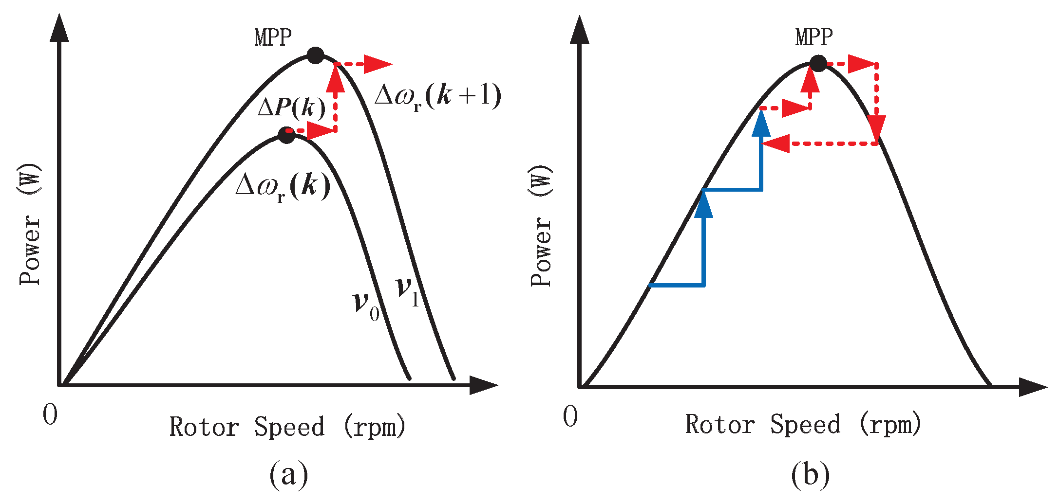
To explain the proposed MPPT strategy, more discussions are given as the following. The power maximization process is shown in Figure 3. It is supposed that the point is a MPP of a certain wind velocity (e.g., ). In this case, , , and are the four operating points, which are randomly chosen around the point . Figure 3 shows the positions of the proposed five operating points in the MPPT curve depicted in Figure 3a and OPC curve depicted in Figure 3b, respectively. It is seen that the value shown in Figure 3b is increased in the high-speed side of the OPC curve, resulting in the rotor speed reduction and power increase illustrated in Figure 3a, until (that is MPP) is reached illustrated in Figure 3b. Similarly when the operating point is starting in the low-speed side, following results in the reduction and the subsequent convergence at (that is MPP) illustrated in Figure 3b, since the rotor speed is progressively increased. Table 1 lists the values of and () for the five observed operating points. If is negative, it means that is less than the optimal rotor speed as shown in Figure 1 and the direction of a perturbation process is continued in the same direction. While, if is positive, it means that is greater than , and the direction of a perturbation process should be reversed.
As known, the model of WECS is a strictly proper real system with unmodeled disturbances and parameter uncertainties [24]. With the nonlinear uncertainty due to the movement of the operating points and disturbances, adequate transient performance cannot be guaranteed using a PI controller as discussed in [9]. Therefore, a novel perturb and observe regulator (POR) is designed to achieve a trade-off between the transient performance and the stability of the MPPT control strategy under disturbances. In order to realize the proposed MPPT strategy, two novel controllers based on the proposed POR, e.g., MPPT controller and speed controller, are proposed in this paper. According to the calculated , it can be found in Figure 1 that the MPPT controller generates the rotor speed reference as the inputs to the speed controller. The objective of the speed controller is to generate the duty cycle reference in order to regulate rotor speed by tracking the reference .
3.2. Estimator of Mechanical Power Coefficient
In practice, the wind turbine power is a quantity that is difficult to measure directly [4]. Additionally, most of the reported MPPT algorithms use the generator power as the feedback power signal input to realize MPPT operations [4,25]. can be calculated by an approximation expression based on (7):
Substituting (21) into (17):
where can be written in terms of the generator rectification current [10]:
Based on (22) and (23), the mechanical power coefficient estimator is designed as shown in Figure 4. As a result, it only requires one current sensor to measure instead of at least two current sensors to measure .
It can be found that the estimator contains, on one side, the information of real-time inductor current and, on the other side, the rotor speed providing the real-time speed information of the studied WECS.
4. Design and Analysis of POR-Based MPPT and Speed Controllers
4.1. Design of POR-Based MPPT and Speed Controllers
A traditional HCS algorithm is commonly based on calculating the gradient of the wind turbine power and rotor speed [10,12], that is . It is required to determine the direction of the next perturbation variable within a sampling time, which is given by:
Based on (24), there is a major drawback of the traditional HCS algorithm that the direction of the perturbation variable can be misled, owing to the fact that the HCS algorithm is blind to a change of wind speed [10]. This scenario is shown in Figure 5a that the misled direction of the HCS algorithm under wind speed changes ( to ). Figure 5b also shows the other problems, e.g., the steady-state oscillations around an MPP and a slow tracking speed.
To solve the tracking direction error under changing wind speeds and decrease the steady-state oscillations around an MPP in an HCS algorithm, a perturb and observe regulator (POR) based on perturbation and observation has been proposed as shown in Figure 6. Two new controllers based on POR, e.g., an MPPT controller and a speed controller, are first proposed in this research. With the concept of the perturb and observe, the MPPT and speed controllers are adopted for estimating the rotor speed reference and the optimal duty cycles , respectively, which can enhance the tracking capabilities of the proposed MPPT strategy by controlling the real-time signals ( or ) to track the signal references ( or ).
Under wind-gust disturbances, the perturbation process of a classic HCS algorithm easily leads to wrong tracking directions as shown in Figure 5a, because the sampling time is generally smaller than the mechanical time constant of a WECS. The main difference between the proposed PORs and a classic HCS algorithm is that the latter is based on calculating the gradient of the wind turbine characteristics (i.e., ), while the former just needs to estimate the signal references ( or ) instead of considering . The control diagrams of the proposed POR-based MPPT and speed controllers, which share the same structure, are shown in Figure 6a,b, respectively.
At first, the input variables ( or ) are first calculated and compared with the reference one ( or ) as the following:
where is the power coefficient difference and is the rotor speed difference.
The two POR-based controllers work in two subsequent processes: an observation process and a perturbation process. Based on the comparisons between (or ) and (or ), the size of the observation is determined according to the following:
where and are the pre-determined thresholds; and are the weight factors, which are positive values used to adjust perturbation step sizes; is the step size determined by and a factor ( or ) designed based on system characteristics.
It can also be found in the observation process that has two kinds of values, (or ) and zero. When is equal to zero in the observation process, the perturbation process is terminated in order to avoid oscillations around operating power points and to decrease overshoots under fast wind speed variations.
The second process is the perturbation process, which is responsible for bringing the operating point to the vicinity of MPP during fast wind speed changes. The perturbation process makes use of (26) and (27) to track the signal reference ( or ) by continuously adjusting the perturbation variable ( or ) to reach the MPP. The process is terminated until is equal to zero.
where .
where .
According to (26) and (27) the direction of the next perturbation step size depends on the sign of (or ).
It should be noted that the duty cycle and inductor current are inherently coupled by the presence of MPPT [26]. This makes the overall coordination of the entire control system challenging. However, owing to the POR-based speed controller designed to include the information of the duty cycle and the estimator for mechanical power coefficient including the inductor current shown in (22), the studied system in this research is particularly simplified without a current loop, and it is just controlled by only one speed loop. Additionally, the corresponding convergence and stability are analysed in the next section.
4.2. Convergence Analysis of the Proposed Speed Controller
A sliding mode (SM) control scheme is typically based on high frequency switching of control signals as discussed in [27,28], which is suitable for power converters [15]. Essentially, the proposed POR-based speed controller has the switch operation mode as shown in (27), which is in agreement with the characteristics discussed in the SM control theory [16,29].
Owing to the nonlinear characteristic of the proposed POR-based speed controller based on the switch operation mode, a duty cycle control law of the SM control is devised to validate the POR-based speed controller, which is capable of driving the studied system to reach a predetermined stable hyperplane. As a result, the convergence of the proposed speed controller can be proven based on the Lyapunov theory as follows.
The hyperplane of the sliding mode designed for the POR-based speed controller is taken as the following:
The constant speed reaching law in (32) is used to get a fast response for reaching the designed hyperplane:
4.3. Stability Analysis of the Proposed Speed Controller
The generator torque of the PMSG can be linearized at the operating point, which is expressed as (11). Additionally, based on (11), (14) and (23), it is concluded that:
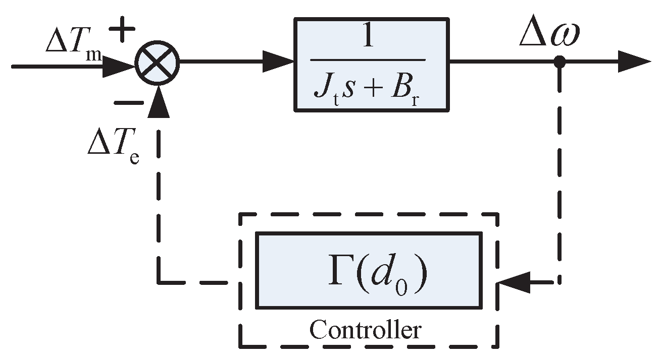
Hence, the wind turbine model linearized at the operating point in (10) with the relationship in (36) is shown in Figure 7.
From Figure 7, the transfer function between the turbine torque and the rotor speed is derived as:
From (37), it can be seen that the studied system has a pole at . Therefore, the duty cycle should be controlled to satisfy the condition in order to stabilize the system dynamics. In this research, is controlled to satisfy the condition of stability.
5. Simulation Verification
In order to verify the POR-based controllers, their performances are compared with a classic HCS-based control strategy of [10], an improved hill climbing searching (IHCS) [13] and a PI-based control strategy (all briefly reviewed in Appendix A). A simulation model based on MATLAB/Simulink is designed and established to implement the four control strategies (the corresponding parameters are displayed in Appendix B).
5.1. Case 1: Step Response of POR-MPPT Control
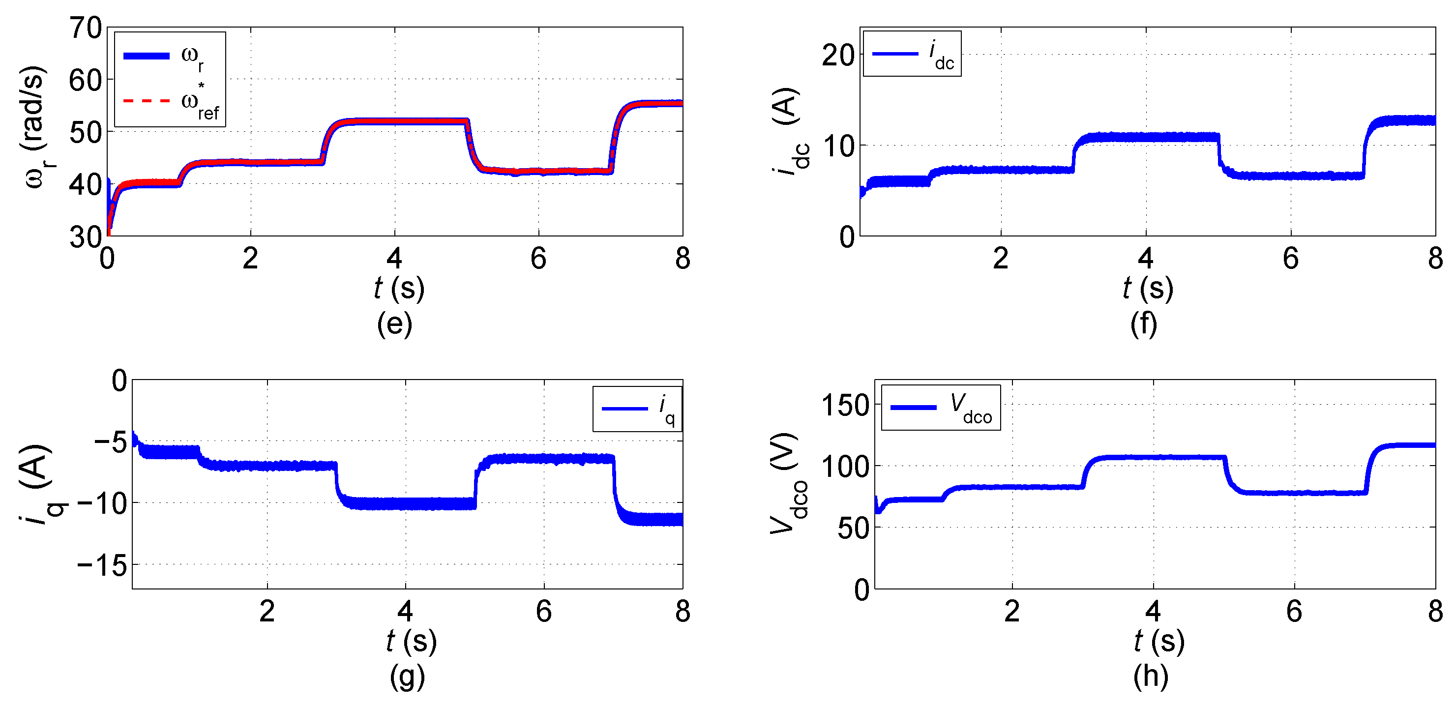
The proposed POR-MPPT control strategy is tested under different step changes of wind speeds shown in Figure 8a. This case study shows the effects of a sudden change of wind speed, similar to the wind shear and tower shadow effects in real operations [9]. The step responses of and are shown in Figure 8b,c respectively. Due to the step change of wind speed, there is a sudden change of , and drops accordingly. Then, is regulated to return to its optimal value quickly (less than 0.3 s) even for large step changes (from 8 to 11 m/s). The reference rotor speed is estimated by means of the proposed MPPT controller shown in Figure 1 described in Section 2. The comparison between the estimated rotor speed and the optimal one is shown in Figure 8d. Also in Figure 8e, the actual rotor speed tracks the estimated one well using the proposed speed controller. Both the proposed POR-based controllers demonstrate superior capabilities of tracking the corresponding reference signals. The inductor current and q axis current waveforms of the studied WECS are also depicted on Figure 8f,g, respectively, to show the relationship between the two currents as described in (23). Moreover, it can be clearly observed that the output voltage curve shown in Figure 8h and the step change wind speeds are in good agreement, which shows that the POR-based controllers can achieve the tracking goals under rapid wind speed variations.
5.2. Case 2: Comparison of the POR-MPPT with HCS and IHCS in Transient Performance
In order to investigate the transient capabilities of the proposed POR-MPPT control strategy under step changes of wind speed conditions, the classic HCS and IHCS methods [13] are compared with the proposed POR-MPPT control strategy.
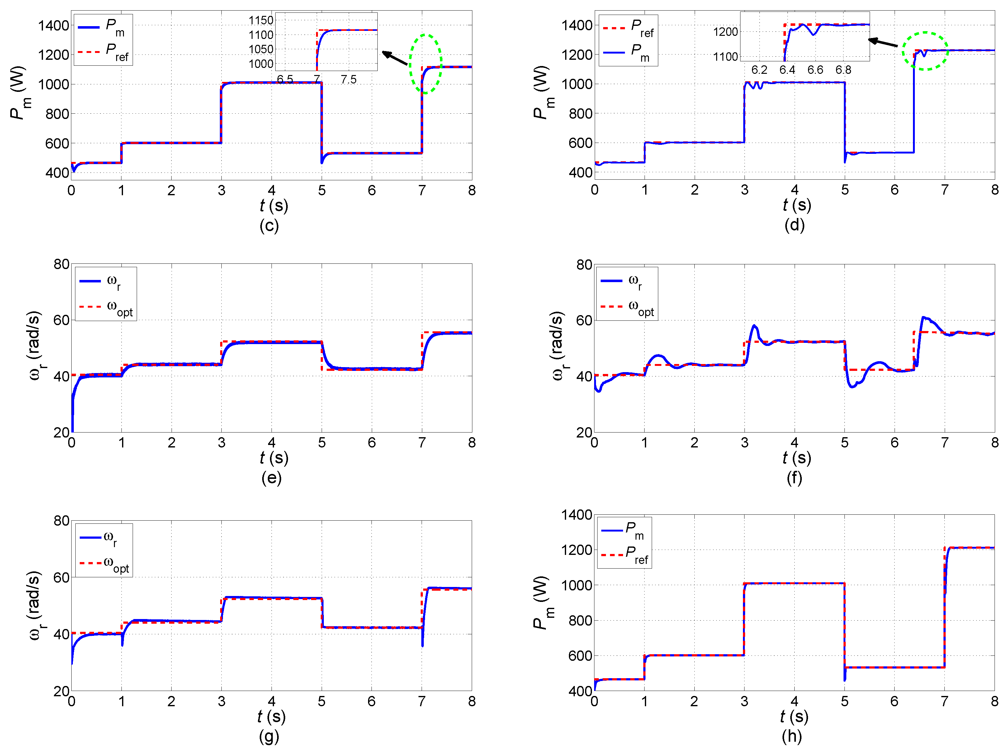
Figure 9a–f shows, respectively, the mechanical power coefficient , the mechanical power , the rotor speed of the proposed POR-MPPT and the classic HCS method. It illustrates that in the two control strategies is controlled to around showing that the MPPT operation is achieved, while the POR-MPPT illustrates a better capability of tracking than that of classic HCS as in Figure 9a,b due to the robust design method included in the former strategy. Figure 9c,d shows, respectively, the dynamic performance of under rapid wind speed changes between the proposed two methods. Compared with the classic HCS method, the variations in the proposed POR-MPPT control strategy show better response during the stepwise change of the wind speed, due to the super tracking performance of , as shown in Figure 9e.
Figure 9g,h shows, respectively, the rotor speed and the mechanical power of the IHCS method. As can be seen in Figure 9g, the rotor speed can barely reach the reference one when the wind speed is changed sharply. However, in the case of the proposed POR-MPPT control method shown in Figure 9e, the rotor speed not only follows its reference well, but also shows faster performance than that of the IHCS method. It can be seen that the dynamic tracking performance of in the POR-MPPT control strategy provides less deviations between references and actual model outputs than that of HCS and IHCS methods, due to the robust design method used in the research.
5.3. Case 3: Model Parameters Uncertainty Verification
With the model uncertainty due to the ageing phenomenon of PMSG and wind harmonics [7] and high temperatures, the model output parameters, e.g., , and , may be changed. Moreover, the parameters , may be changed because of changed temperatures. Accurate transient performance cannot be guaranteed using a traditional PI controller [9]. Therefore, the proposed robust controllers are employed to tackle such problems.
To model the wind harmonics, the wind speed variation is modelled by a trapezoidal pattern shown in Figure 10b as given by [7],
where is the wind speed base function, as shown in Figure 10a.
To model the ageing phenomenon, the tracking performance of the system is studied for the flux strength of 85% of the rated value and compared with the tracking performance under the rated flux . Figure 10c,d shows the simulation results of both the PI and POR control systems with respect to errors in the PM flux using the reference wind speed in Figure 10b. As Figure 10d shows, the POR control system accurately tracks the reference input in the case of , while in Figure 10c, the PI control system fails to track the reference during the time of 4 to 12 s and 17 to 26 s under the same conditions. These study results also confirm the robustness capabilities of the POR-based controller compared with PI.
To model the impact of high temperature on the PMSG parameters, the values of resistance and inductance applied to the studied PMSG are, respectively, adjusted to and . Figure 11a,b shows the simulation results of both the proposed POR-based and PI controllers with respect to variations in , when the wind speed changes from 9 m/s to 14 m/s at 5 s and back to 10 m/s at 20 s. Figure 11b shows that the POR-based controller accurately tracks the reference input for and . However, the PI controller fails to achieve the tracking goals for and in Figure 11a.
To model the impact of changed temperature on , the value of is produced by a random signal generator as shown in Figure 11c. According to (19) and (20), the mechanical power reference is changed according to the different value of . Figure 11d shows the simulation results that the POR-based controller can achieve the tracking goals even during variation of the reference signal, which displays an excellent tracking performance of the proposed POR-based controller.
5.4. Case 4: Maximum Power Extraction under Random Wind Speeds
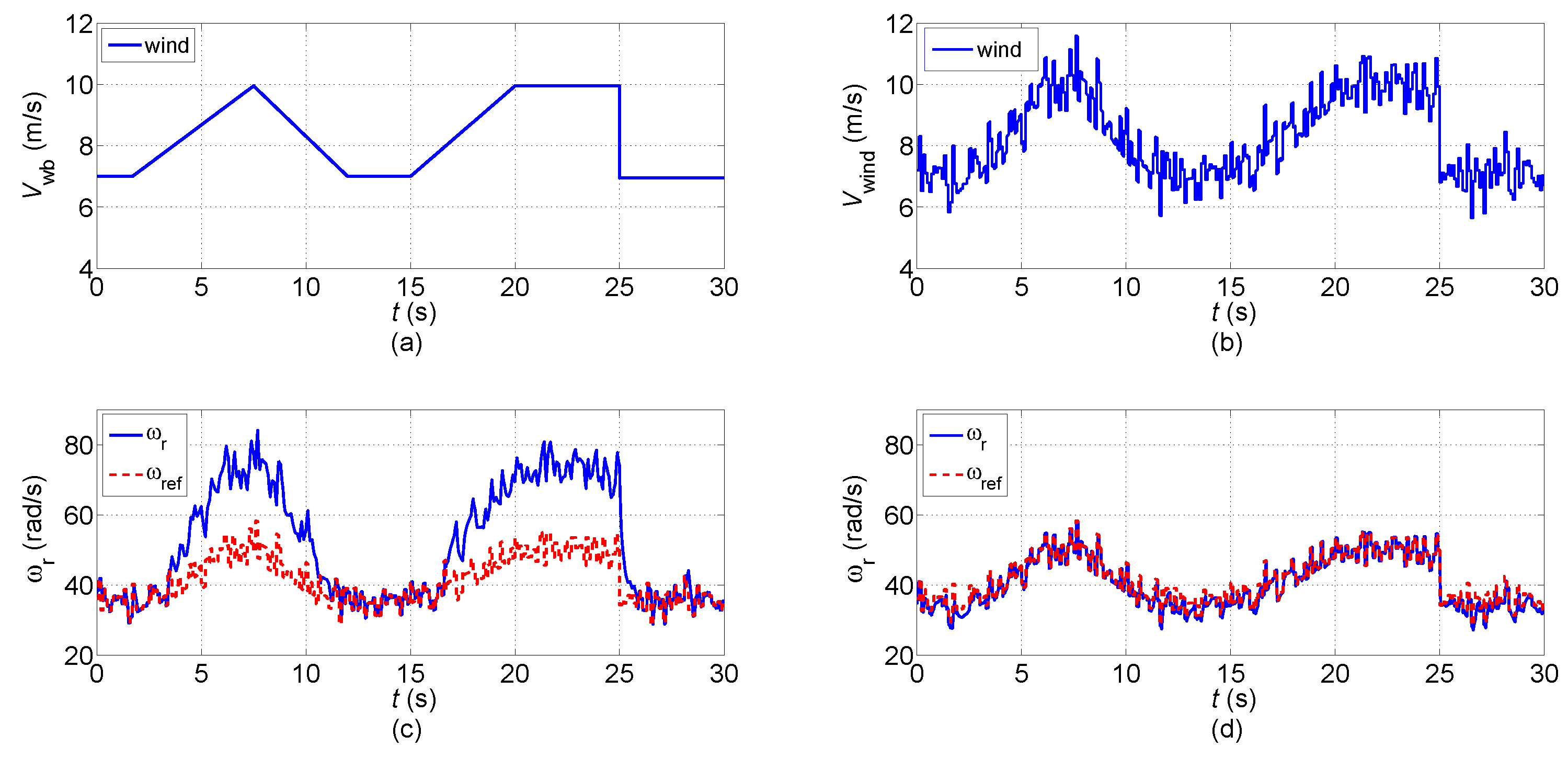
The objective of this section is to validate the capability of the proposed POR-MPPT for maximum power extractions. This case is divided into Scenarios 1 and 2 based on the different turbulence intensities of wind profiles as shown in Figure 12a,e, respectively. In the simulation, wind speed profiles with a frequency of 3 Hz (wind speeds change three times per second) and 6 Hz are adopted in Scenario 1 and 2, respectively. Considering the time-varying viscous coefficients and disturbances, the wind profiles are randomly generated to simulate actual wind speeds. The mean and variance of wind speeds are set as 9 m/s and 1 m/s, respectively. In this research, the percentage absolute average power deviations defined as AAPD% for Case 4 are computed by (39) and listed in Table 2.
where is the optimal mechanical power, .
Time-domain simulations are carried out for the studied WECS in Figure 12 among the proposed four control methods, e.g., the proposed POR-MPPT, the classic HCS, IHCS and PI methods. Figure 12b–d shows the mechanical power loss among the four methods under the 3-Hz random wind speed conditions (Scenario 1), while Figure 12f,g,h displays, respectively, among the four methods under the 6-Hz random wind speed conditions (Scenario 2). Specially, Figure 12d,h illustrates the detailed comparison results between the POR-MPPT and IHCS methods under the two scenarios. The POR-MPPT has a superior dynamic tracking performance than that of other three methods, as shown in Figure 12. It can be clearly observed that the POR-MPPT method can acquire the largest maximum power extractions among the proposed four methods in Table 2.
6. Experimental Verification
To demonstrate the validity of the proposed POR-MPPT algorithm, an experiment is carried out for a 0.5-kW PMSG wind turbine simulator. The experimental setup in the laboratory is shown in Figure 13. The squirrel-cage induction motor (SCIM) is driven by an alternating current (AC) drive inverter, where the demand is given by the wind turbine simulator (WTS). A controlled DC/DC converter is used to realize the proposed POR-MPPT algorithm based on a TMS320F28335 digital signal processor (DSP) controller. The parameters of the turbine and PMSG are listed in Appendix C, respectively.
Figure 14 shows, respectively, the stable responses of inductor current , the line current of PMSG and the line voltage of PMSG by the POR-MPPT control method, when the wind speed is a constant value of 16 m/s. It is obvious that the waveforms of and are affected by harmonic distortion due to the function of an uncontrolled rectifier diode.
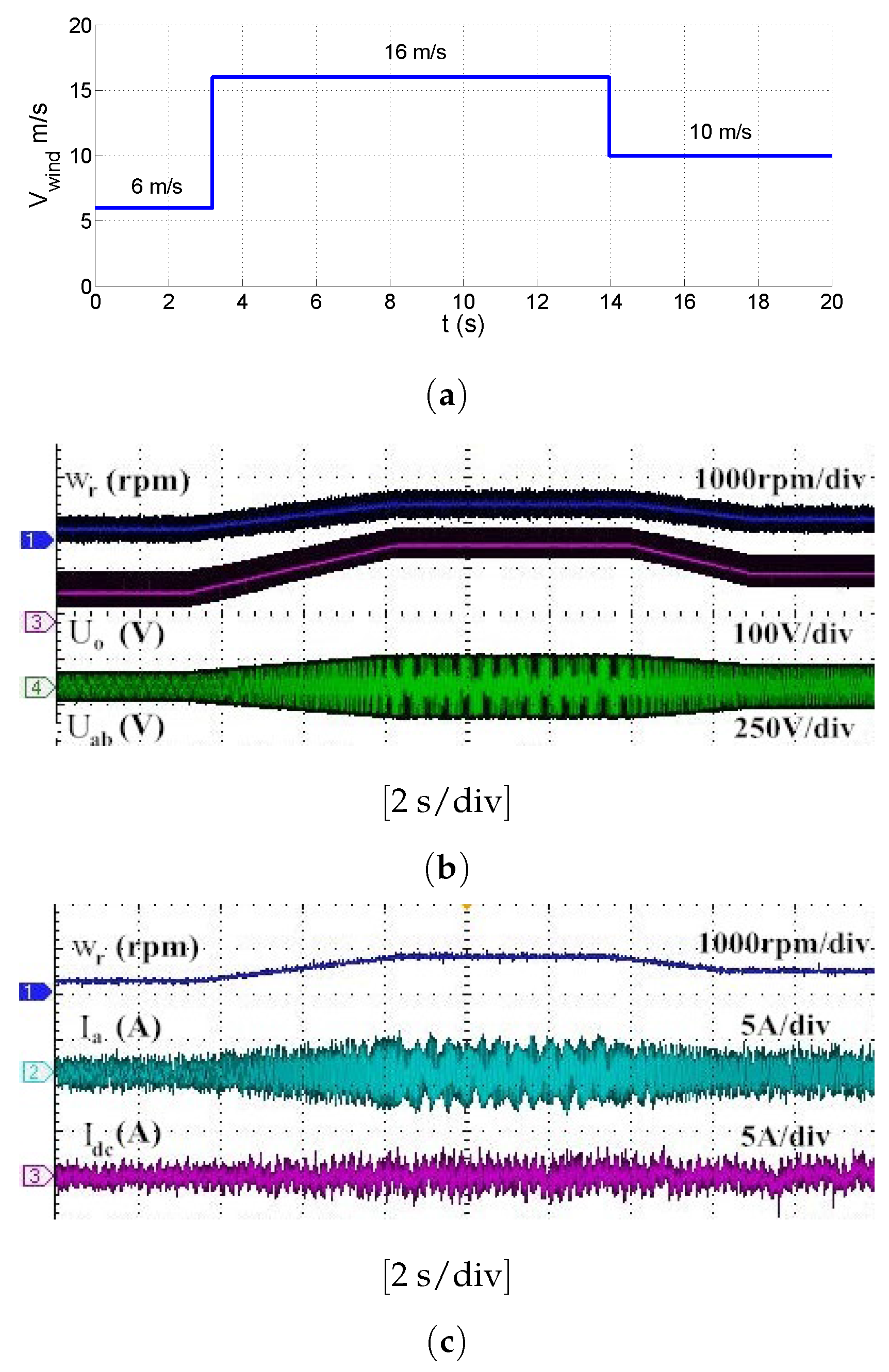
Figure 15 illustrates the dynamic responses of the POR-MPPT control method when the wind speed changes from 6 to 16 m/s and back to 10 m/s. According to optimal tip speed ratio described in (3), the optimal rotor speeds of 6 m/s, 16 m/s, 10 m/s are 30.2 rad/s (equal to 288.4 revolutions per minute (rpm)), 80.5 rad/s (equal to 768.8 rpm) and 50.3 rad/s (equal to 480.4 rpm), respectively. In terms of the scale of rpm shown in Figure 15b,c, it can be calculated that the actual rotor speed (rpm) can track the corresponding optimal rotor speed, which shows that the POR-based controllers can achieve the tracking goals under rapid wind speed variations. The load voltages , , and are also shown in Figure 15b,c, as well. It can be clearly observed that curve and rotor speed changes shown in Figure 15b are in good agreement in terms of (13), which demonstrates the validity of Figure 8d,h in Section 5.1.
7. Conclusions
By combining the perturbation and observation method with the theory of SM, the proposed POR-based controllers are designed based on the linearized WECS model in order to achieve a trade-off between the transient performance and the stability of the MPPT under disturbances. The proposed control system is particularly simplified without a current loop and is just controlled by a speed loop because of the proposed estimator designed to include the information of inductor current. This research proposes a novel OPC instead of the traditional MPPT curve to realize the MPPT operation. It dramatically improves the tracking performance of control system based on the OPC. Compared with the PI, HCS and IHCS methods, the proposed POR-based controllers demonstrate an excellent tracking performance and robustness with fast adaptation to uncertainties and disturbances, as shown in simulation and experimental cases.
Acknowledgments
The project is supported by the National Natural Science Foundation of China (No. 51477054).
Author Contributions
Bo Li designed the proposed robust regulator, performed the analysis and simulation results. Wenhu Tang, Kaishun Xiahou and Qinghua Wu were the advisors of Bo Li. All authors have contributed significantly to this work.
Conflicts of Interest
The authors declare no conflict of interest.
Nomenclature
Air density () | |
| A | Effective area swept by wind turbine () |
Wind turbine power conversion coefficient | |
Maximum value of wind turbine power conversion coefficient | |
| r | Turbine radius () |
Rotor speed of turbine () | |
Tip speed ratio | |
Optimal value of tip speed ratio | |
Pitch angle | |
components of the stator voltage () | |
components of the stator current () | |
components of the stator inductances () | |
Stator resistance () | |
| p | Number of machine poles |
Permanent magnet flux linkage () | |
Wind turbine torque () | |
Generator torque () | |
Rotor inertia () | |
Damping coefficient | |
Generator rectification voltage () | |
Inductor current () | |
| d | Duty cycle |
Generator rectification voltage constant | |
Mechanical power coefficient | |
Optimal power constant | |
Power coefficient difference | |
Rotor speed difference () | |
Pre-determined thresholds | |
Weight factors | |
Step size | |
Optimal mechanical power () | |
| R | Load resistance () |
Appendix A. Conventional PI-Based, HCS-Based and IHCS-Based Control Strategies
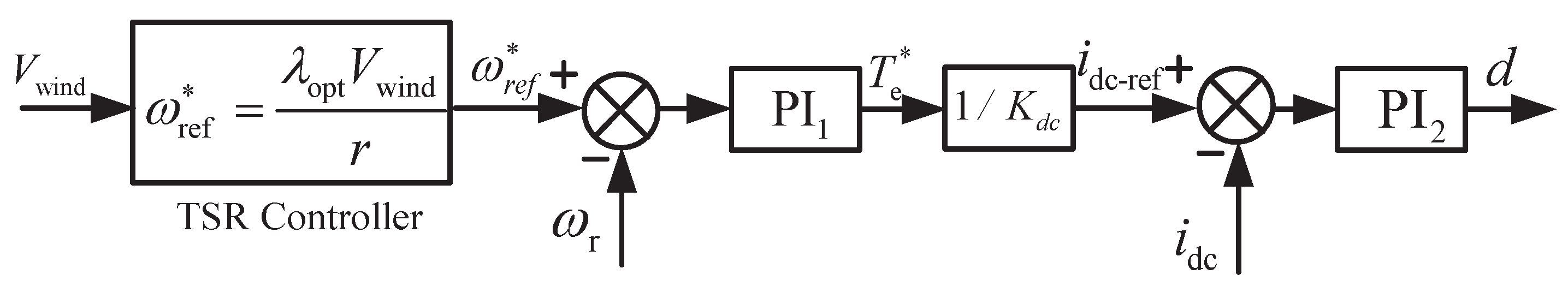
Appendix A.1. PI-Based Control Strategy
The conventional PI-based control strategy consists of a rotor loop to generate the torque reference by the controller, and a current loop to generate an optimal duty cycle d by the controller, as shown in Figure A1. The rotor speed reference is calculated by a TSR controller by measuring wind speeds .
Figure A1.
Block diagram of the PI-based control strategy.
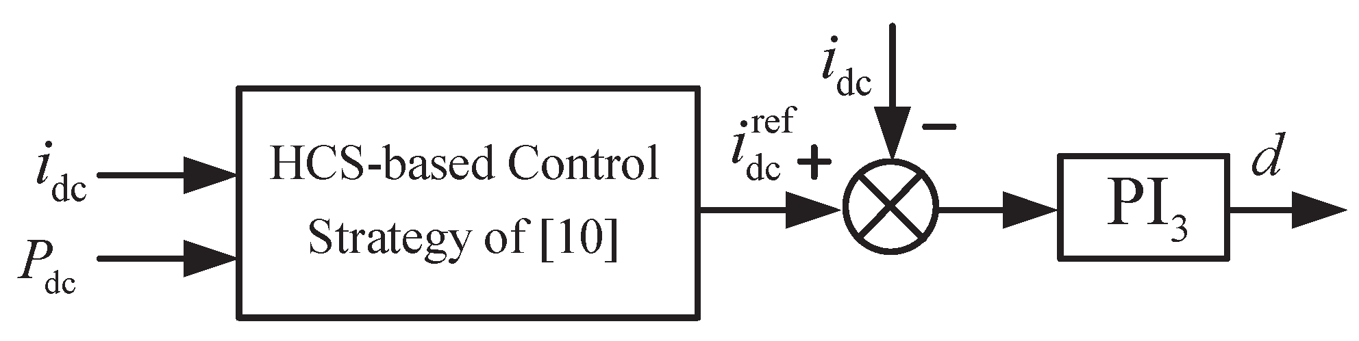
Appendix A.2. HCS-Based Control Strategy
The HCS-based control strategy is shown in Figure A2. It consists of a classic HSC-based control strategy designed for MPPT operations and the current loop controlled by the controller to generate an optimal duty cycle d.
Figure A2.
Block diagram of the HCS-based control strategy.
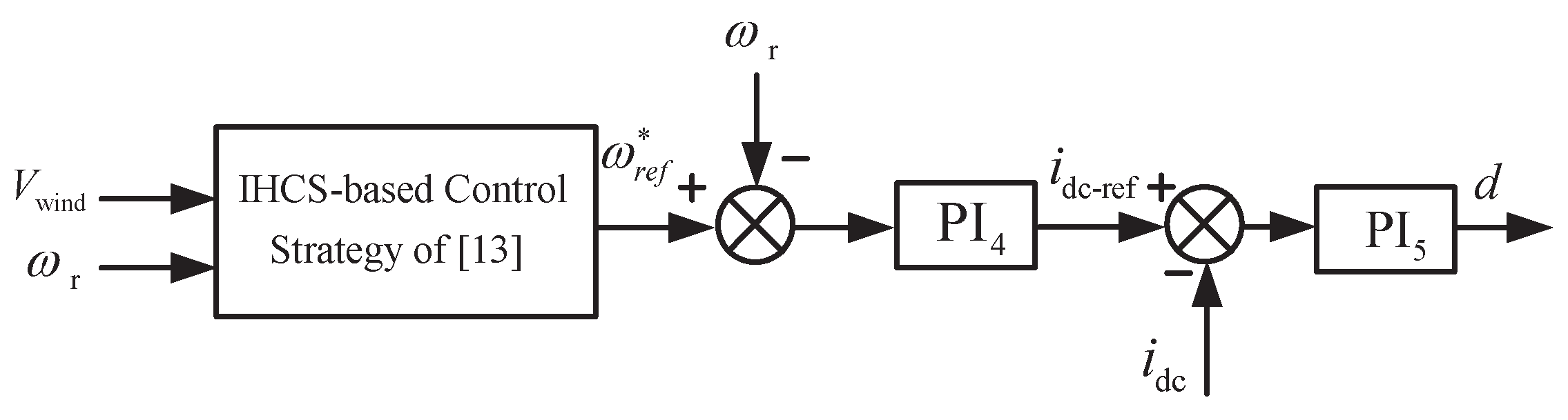
Appendix A.3. IHCS-Based Control Strategy
The IHCS-based control strategy is shown in Figure A3. It consists of an IHCS-based control strategy designed for MPPT operations and the rotor loop controlled by the controller to generate an optimal duty cycle d.
Figure A3.
Block diagram of the IHCS-based control strategy.
Appendix B. Parameters of the Studied WECS for Simulation
(1) Wind turbine parameters in [20]: , , , , , , , .
(2) PMSG parameters in [20]: , , , , .
(3) Converter parameters in [20]: , , , , , d = 0.02.
(4) POR-based control strategy parameters: , , , .
(5) PI-based control strategy parameters: , , , , .
(6) HCS-based control strategy parameters: , , .
Appendix C. Parameters of the Studied WECS for Experiment
(1) Wind turbine parameters: , , , , , .
(2) PMSG parameters: , , , , .
(3) Converter parameters: , , , , .
References
- Liserre, M.; Cardenas, R.; Molinas, M.; Rodriguez, J. Overview of multi-MW wind turbines and wind parks. IEEE Trans. Ind. Electron. 2011, 58, 1081–1095. [Google Scholar] [CrossRef]
- Zou, Y.; Elbuluk, M.E.; Sozer, Y. Stability analysis of maximum power point tracking (MPPT) method in wind power systems. IEEE Trans. Ind. Appl. 2013, 49, 1129–1136. [Google Scholar] [CrossRef]
- Ramasamy, B.; Palaniappan, A.; Yakoh, S. Direct-drive low-speed wind energy conversion system incorporating axial-type permanent magnet generator and Z-source inverter with sensorless maximum power point tracking controller. IET Renew. Power Generat. 2013, 7, 284–295. [Google Scholar] [CrossRef]
- Chen, J.; Chen, J.; Gong, C. New overall power control strategy for variable-speed fixed-pitch wind turbines within the whole wind velocity range. IEEE Trans. Ind. Electron. 2013, 60, 2652–2660. [Google Scholar] [CrossRef]
- Kim, K.H.; Lee, D.C.; Kim, J.M. Fast tracking control for maximum output power in wind turbine systems. In Proceedings of the 2010 20th Australasian Universities Power Engineering Conference (AUPEC), Sydney, Australia, 5–8 December 2010. [Google Scholar]
- Kim, K.H.; Van, T.L.; Lee, D.C.; Song, S.H.; Kim, E.H. Maximum output power tracking control in variable-speed wind turbine systems considering rotor inertial power. IEEE Trans. Ind. Electron. 2013, 60, 3207–3217. [Google Scholar] [CrossRef]
- Ghasemi, S.; Tabesh, A.; Askari-Marnani, J. Application of fractional calculus theory to robust controller design for wind turbine generators. IEEE Trans. Energy Convers. 2014, 29, 780–787. [Google Scholar] [CrossRef]
- Satpathy, A.S.; Kishore, N.; Kastha, D.; Sahoo, N. Control scheme for a stand-alone wind energy conversion system. IEEE Trans. Energy Convers. 2014, 29, 418–425. [Google Scholar]
- Zhao, H.; Wu, Q.; Rasmussen, C.N.; Blanke, M. L1 Adaptive speed control of a small wind energy conversion system for maximum power point tracking. IEEE Trans. Energy Convers. 2014, 29, 576–584. [Google Scholar] [CrossRef]
- Dalala, Z.M.; Zahid, Z.U.; Yu, W.; Cho, Y.; Lai, J.S.J. Design and analysis of an MPPT technique for small-scale wind energy conversion systems. IEEE Trans. Energy Convers. 2013, 28, 756–767. [Google Scholar] [CrossRef]
- Koutroulis, E.; Kalaitzakis, K. Design of a maximum power tracking system for wind-energy-conversion applications. IEEE Trans. Ind. Electron. 2006, 53, 486–494. [Google Scholar] [CrossRef]
- Datta, R.; Ranganathan, V.T. A method of tracking the peak power points for a variable speed wind energy conversion system. IEEE Trans. Energy Convers. 2003, 18, 163–168. [Google Scholar] [CrossRef]
- Heo, S.Y.; Kim, M.K.; Choi, J.W. Hybrid intelligent control method to improve the frequency support capability of wind energy conversion systems. Energies 2015, 8, 11430–11451. [Google Scholar] [CrossRef]
- Zhang, D.; Wang, Y.; Hu, J.; Ma, S.; He, Q.; Guo, Q. Impacts of PLL on the DFIG-based WTG’s electromechanical response under transient conditions: Analysis and modelling. CSEE J. Power Energy Syst. 2016, 2, 30–39. [Google Scholar] [CrossRef]
- Corradini, M.L.; Ippoliti, G.; Orlando, G. Robust control of variable-speed wind turbines based on an aerodynamic torque observer. IEEE Trans. Control Syst. Technol. 2013, 21, 1199–1206. [Google Scholar] [CrossRef]
- Beltran, B.; Benbouzid, M.E.H.; Ahmed-Ali, T. Second-order sliding mode control of a doubly fed induction generator driven wind turbine. IEEE Trans. Energy Convers. 2012, 27, 261–269. [Google Scholar] [CrossRef]
- Zhu, Y.; Cheng, M.; Hua, W.; Wang, W. A novel maximum power point tracking control for permanent magnet direct drive wind energy conversion systems. Energies 2012, 5, 1398–1412. [Google Scholar] [CrossRef]
- Phan, D.C.; Yamamoto, S. Maximum energy output of a DFIG wind turbine using an improved MPPT-curve method. Energies 2015, 8, 11718–11736. [Google Scholar] [CrossRef]
- Pan, C.T.; Juan, Y.L. A novel sensorless MPPT controller for a high-efficiency microscale wind power generation system. IEEE Trans. Energy Convers. 2010, 25, 207–216. [Google Scholar]
- Mahadi, A.; Tang, W.H.; Wu, Q.H. Derivation of a complete transfer function for a wind turbine generator system by experiments. In Proceedings of the 2011 IEEE Power Engineering and Automation Conference (PEAM), Wuhan, China, 8–9 September 2011; pp. 35–38. [Google Scholar]
- Tang, W.H.; Wu, Q.H.; Mahdi, A.J. Parameter identification of a PMSG using a PSO algorithm based on experimental tests. In Proceedings of the 2010 1st International Conference on Energy, Power and Control (EPC-IQ), Basra, Iraq, 30 November–2 December 2010. [Google Scholar]
- Kotti, R.; Shireen, W. Maximum power point tracking of a variable speed PMSG wind power system with DC link reduction technique. In Proceedings of the 2014 IEEE PES General Meeting, Conference & Exposition, Washington, DC, USA, 27–31 July 2014. [Google Scholar]
- Jeong, H.G.; Seung, R.H.; Lee, K.B. An improved maximum power point tracking method for wind power systems. Energies 2012, 5, 1339–1354. [Google Scholar] [CrossRef]
- Billy, P.; Muhando, E.; Senjyu, T.; Uehara, A.; Funabashi, T. Gain-Scheduled H∞ control for WECS via LMI techniques and parametrically dependent feedback Part I: model development fundamentals. IEEE Trans. Ind. Electron. 2011, 58, 48–56. [Google Scholar]
- Kazmi, S.M.R.; Goto, H.; Guo, H.J.; Ichinokura, O. A novel algorithm for fast and efficient speed-sensorless maximum power point tracking in wind energy conversion systems. IEEE Trans. Ind. Electron. 2011, 58, 29–36. [Google Scholar] [CrossRef]
- Pucci, M. Induction machines sensors-less wind generator with integrated intelligent maximum power point tracking and electric losses minimisation technique. IET Control Theory Appl. 2015, 9, 1831–1838. [Google Scholar] [CrossRef]
- Utkin, V.; Guldner, J.; Shi, J. Sliding Mode Control in Electro-Mechanical Systems; CRC Press: Boca Raton, FL, USA, 2009. [Google Scholar]
- Bartolini, G.; Orani, N.; Pisano, A.; Usai, E. Higher-order sliding mode approaches for control and estimation in electrical drives. In Advances in Variable Structure and Sliding Mode Control; Springer: Berlin/Heidelberg, Gemany, 2006; pp. 423–445. [Google Scholar]
- Feng, Y.; Zheng, J.; Yu, X.; Truong, N.V. Hybrid terminal sliding-mode observer design method for a permanent-magnet synchronous motor control system. IEEE Trans. Ind. Electron. 2009, 56, 3424–3431. [Google Scholar] [CrossRef]
Figure 1.
Block diagram-system configuration of the proposed MPPT algorithm.
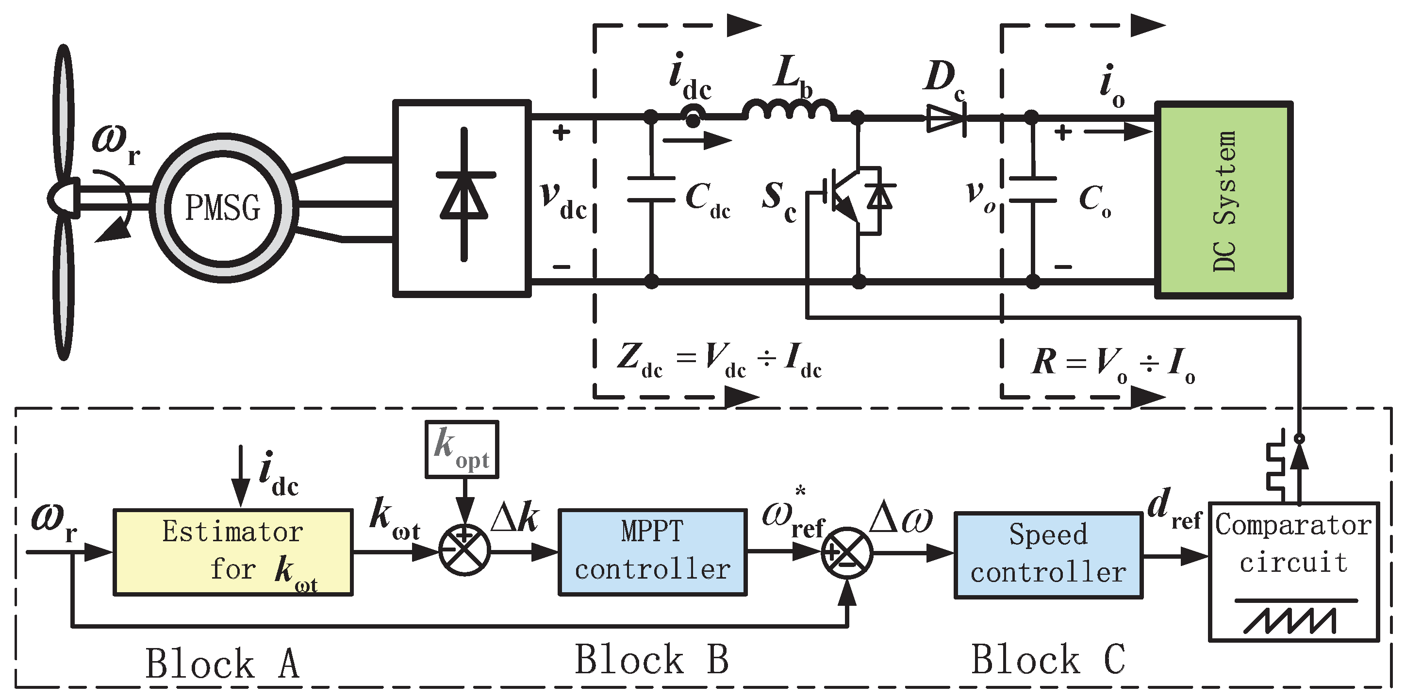
Figure 2.
Mechanical power coefficient as a function of the rotor speed at various wind speeds.
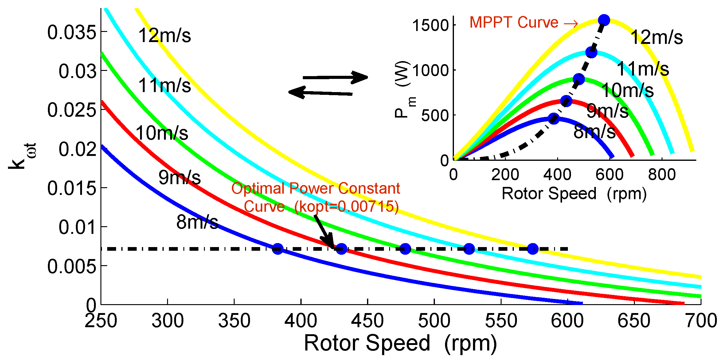
Figure 3.
Operational principle of the proposed MPPT strategy: (a) Operating points in MPPT curve; (b) Operating points in OPC curve.
Figure 3.
Operational principle of the proposed MPPT strategy: (a) Operating points in MPPT curve; (b) Operating points in OPC curve.
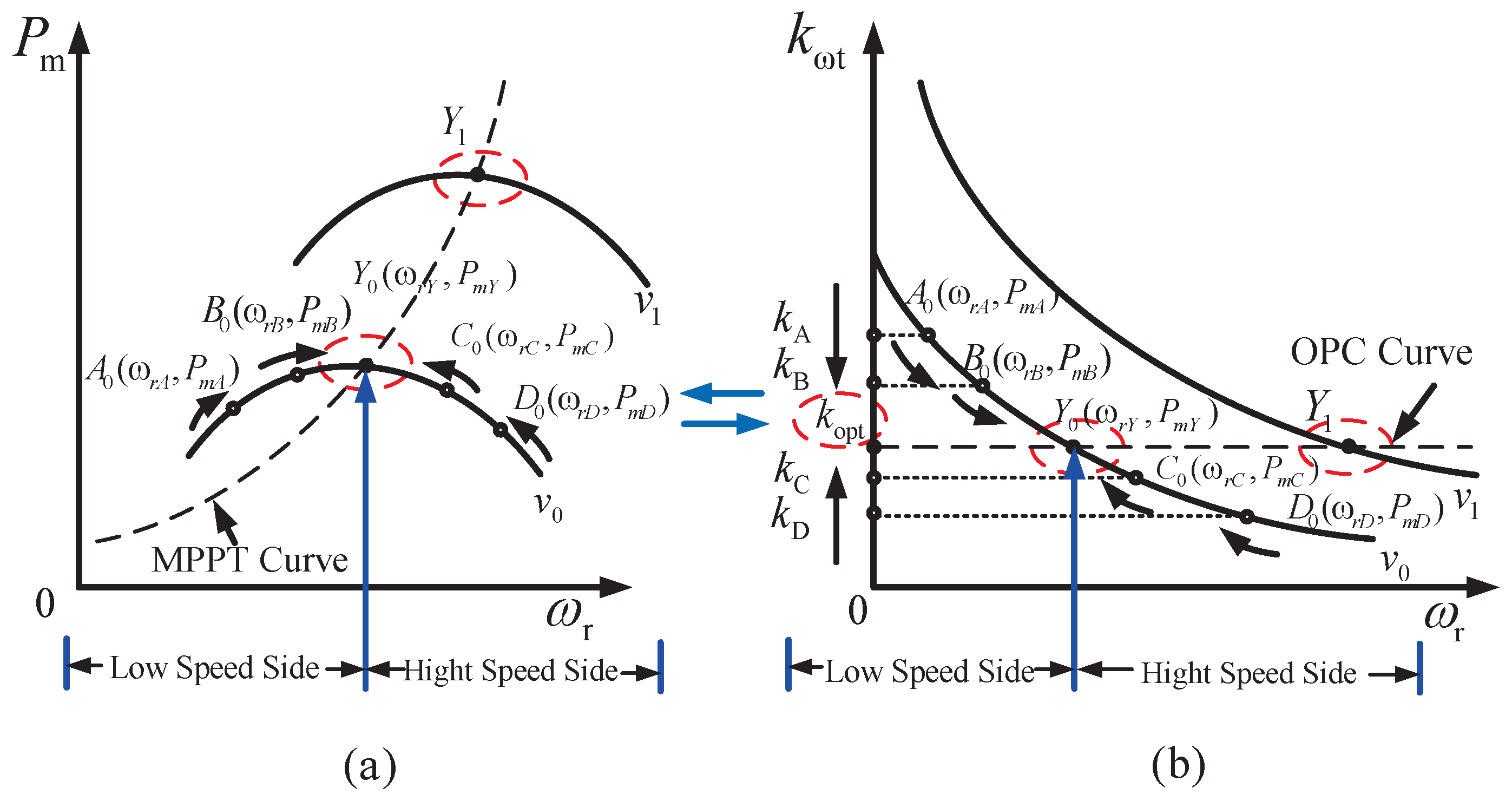
Figure 4.
Estimator of mechanical power coefficient.
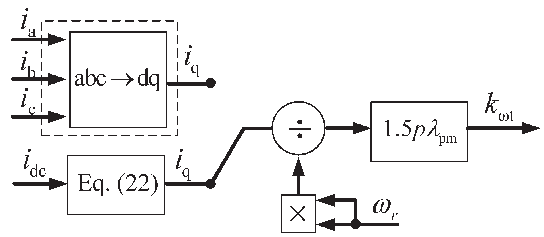
Figure 5.
(a) HCS algorithm direction misled under wind speed changes; (b) HCS algorithm oscillates around the MPP.
Figure 5.
(a) HCS algorithm direction misled under wind speed changes; (b) HCS algorithm oscillates around the MPP.

Figure 6.
(a) Flowchart of the POR-based MPPT controller for estimating ; (b) Flowchart of the POR-based speed controller for estimating .
Figure 6.
(a) Flowchart of the POR-based MPPT controller for estimating ; (b) Flowchart of the POR-based speed controller for estimating .
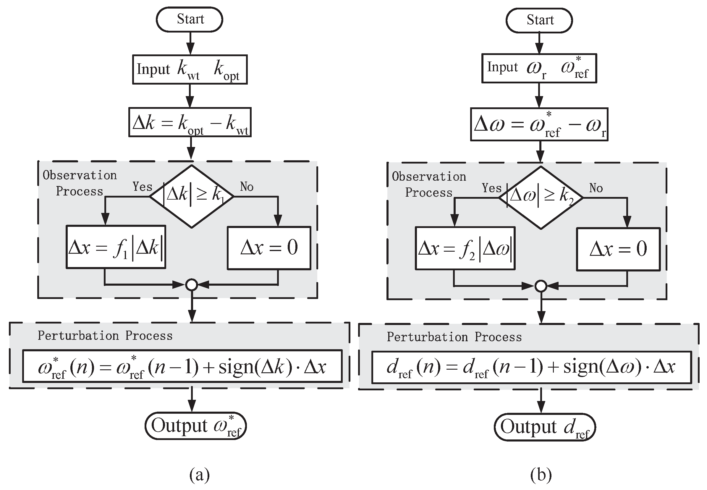
Figure 7.
Small signal analysis of generator torque including the speed controller.

Figure 8.
Dynamic responses of the PORs under step changes of wind speeds: (a) Wind speed; (b) Power coefficient; (c) Tip speed ratio; (d) Rotor speed; (e) Rotor speed; (f) Inductor current; (g) q axis current; and (h) Output voltage.
Figure 8.
Dynamic responses of the PORs under step changes of wind speeds: (a) Wind speed; (b) Power coefficient; (c) Tip speed ratio; (d) Rotor speed; (e) Rotor speed; (f) Inductor current; (g) q axis current; and (h) Output voltage.
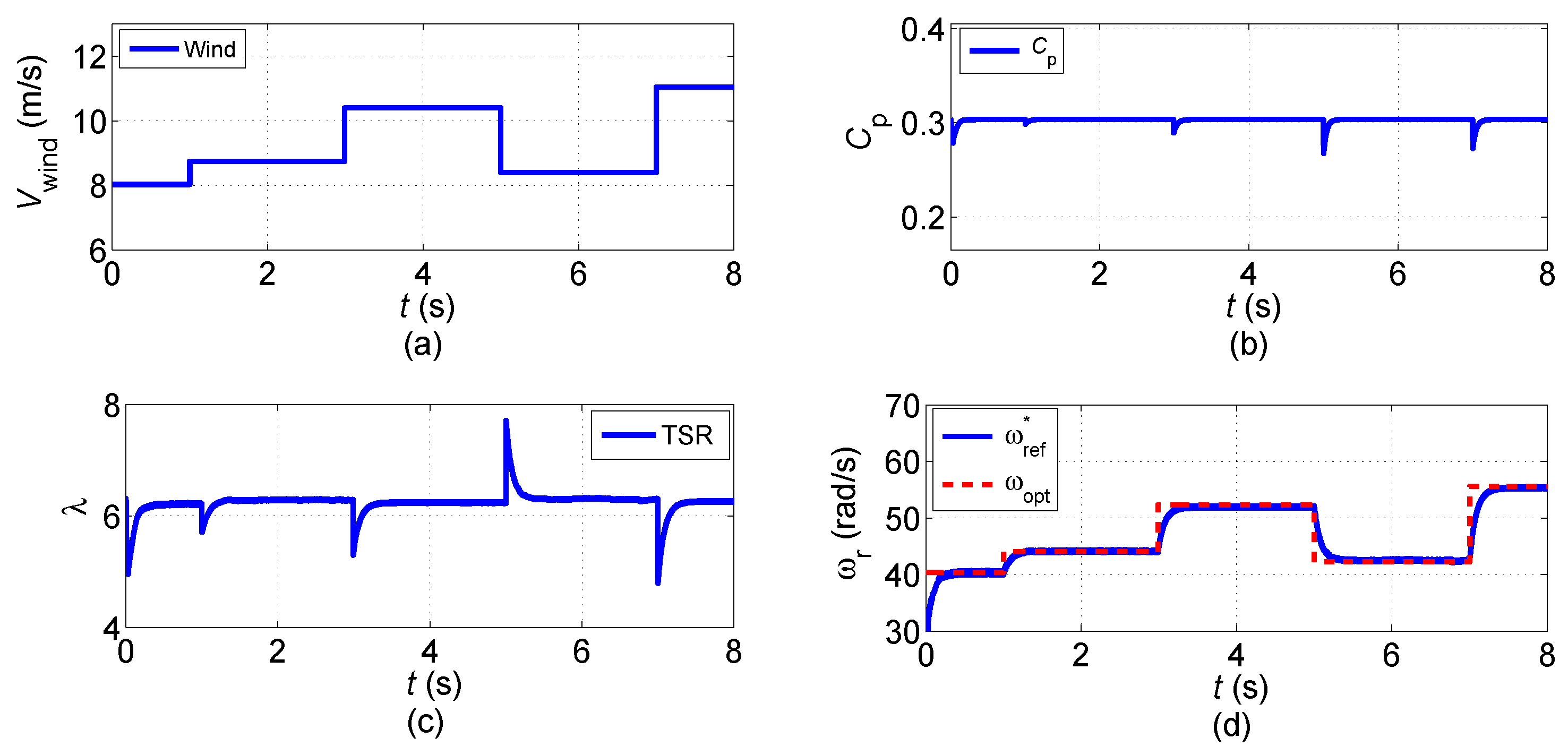

Figure 9.
Dynamic performances compared among the POR-MPPT, classic HCS and IHCS methods under step changes of wind speeds: (a) in POR-MPPT; (b) in HCS; (c) in POR-MPPT; (d) in HCS; (e) in POR-MPPT; (f) in HCS; (g) in IHCS; and (h) in IHCS.
Figure 9.
Dynamic performances compared among the POR-MPPT, classic HCS and IHCS methods under step changes of wind speeds: (a) in POR-MPPT; (b) in HCS; (c) in POR-MPPT; (d) in HCS; (e) in POR-MPPT; (f) in HCS; (g) in IHCS; and (h) in IHCS.


Figure 10.
Robustness of the controllers against wind harmonics, PM aging phenomenon: (a) Wind speed; (b) Wind speed; (c) With 85% errors in PI; and (d) With 85% errors in POR.
Figure 10.
Robustness of the controllers against wind harmonics, PM aging phenomenon: (a) Wind speed; (b) Wind speed; (c) With 85% errors in PI; and (d) With 85% errors in POR.

Figure 11.
Robustness of the controllers against changed temperature under step wind speeds: (a) With −15% and +15% errors in PI; (b) With -15% and +15% errors in POR; (c) Random changed ; and (d) With random changed in POR.
Figure 11.
Robustness of the controllers against changed temperature under step wind speeds: (a) With −15% and +15% errors in PI; (b) With -15% and +15% errors in POR; (c) Random changed ; and (d) With random changed in POR.

Figure 12.
Maximum power extraction under random wind speeds: (a) 3 Hz wind speed variations; (b) under 3 Hz variations between POR-MPPT and HCS; (c) under 3 Hz variations between POR-MPPT and PI; (d) under 3 Hz variations between POR-MPPT and IHCS; (e) 6 Hz wind speed variations; (f) under 6 Hz variations between POR-MPPT and HCS; (g) under 6 Hz variations between POR-MPPT and PI; and (h) under 6 Hz variations between POR-MPPT and IHCS.
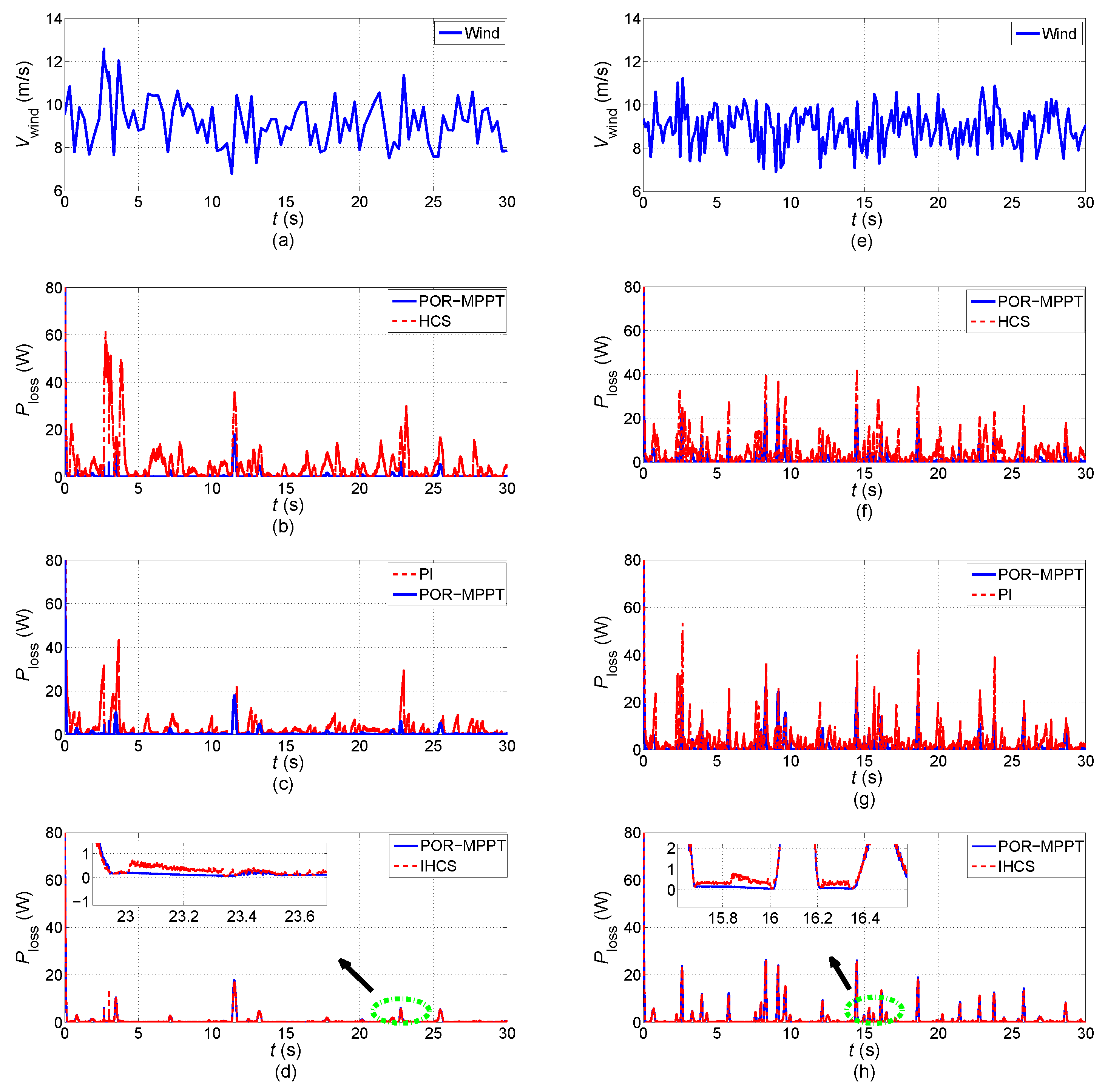
Figure 13.
Layout of the experimental equipment. SCIM: squirrel-cage induction motor.
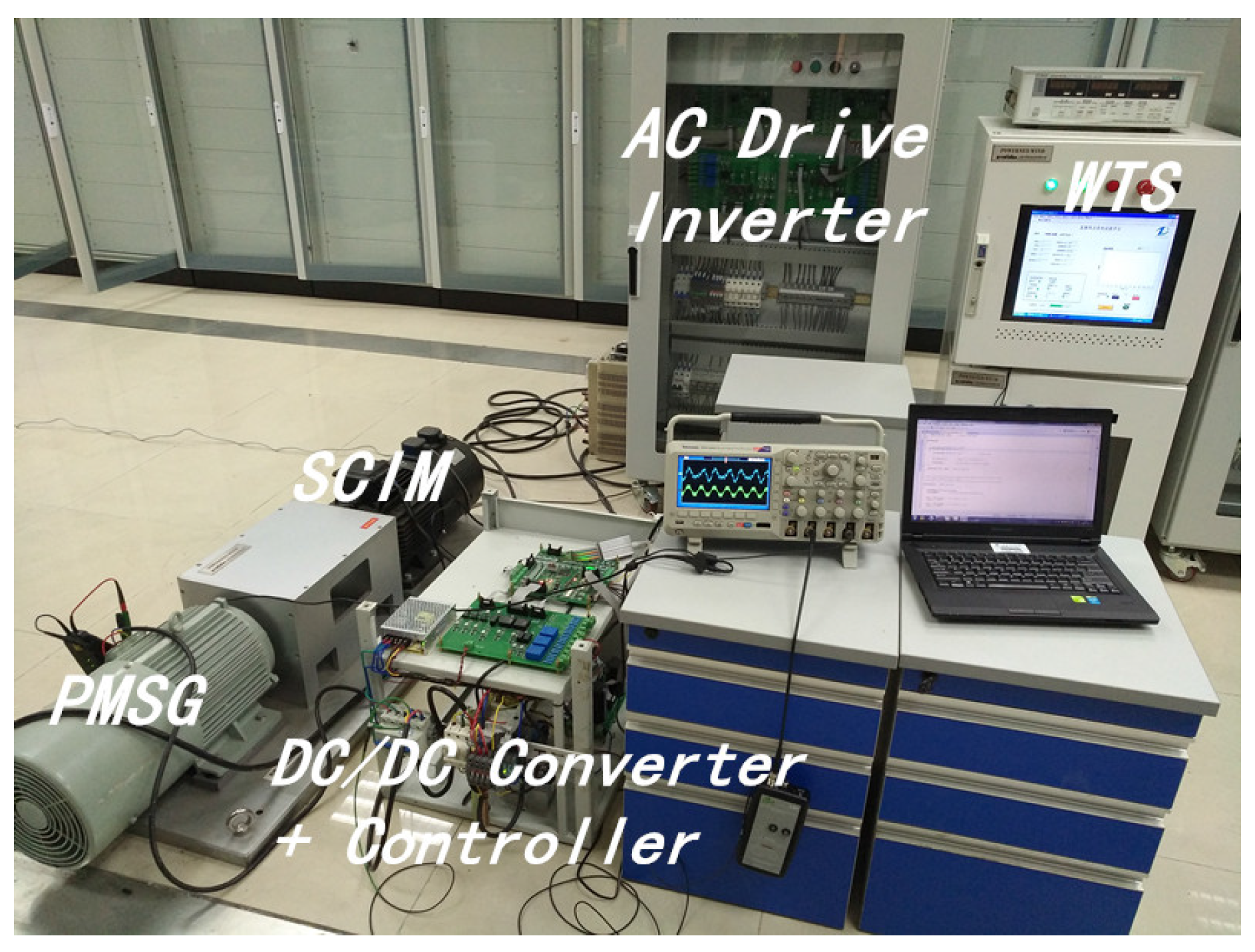
Figure 14.
Responses of POR control in 16-m/s wind speed. (a) Inductor current; (b) Line current and line voltage.
Figure 14.
Responses of POR control in 16-m/s wind speed. (a) Inductor current; (b) Line current and line voltage.
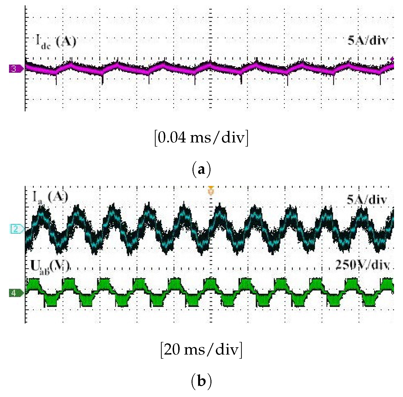
Figure 15.
Responses of POR control in stepwise wind speed variation. (a) Wind speed; (b) Rotor speed, output voltage and line voltage; and (c) Rotor speed, line current and inductor current.
Figure 15.
Responses of POR control in stepwise wind speed variation. (a) Wind speed; (b) Rotor speed, output voltage and line voltage; and (c) Rotor speed, line current and inductor current.

Table 1.
Values of the proposed five power points at the rated wind speed of 10 m/s.
| Power Point | (rad/s) | (W) | ||
|---|---|---|---|---|
| A (Left side) | 37 | 700 | 0.0138 | <0 |
| B (Left side) | 45 | 800 | 0.0088 | <0 |
| (MPP) | 52 | 828 | 0.00705 | =0 |
| C (Right side) | 60 | 800 | 0.0037 | >0 |
| D (Right side) | 66 | 700 | 0.0024 | >0 |
Table 2.
Percentage absolute average power deviations (AAPD%) of mechanical power under random wind speeds.
Table 2.
Percentage absolute average power deviations (AAPD%) of mechanical power under random wind speeds.
| Rate of Change (Hz) | AAPD% of Mechanical Power | |||
|---|---|---|---|---|
| POR | PI | HCS | IHCS | |
| 3 | 1.32% | 2.69% | 3.93% | 1.45% |
| 6 | 1.57% | 3.77% | 4.31% | 1.65% |
© 2017 by the authors. Licensee MDPI, Basel, Switzerland. This article is an open access article distributed under the terms and conditions of the Creative Commons Attribution (CC BY) license (http://creativecommons.org/licenses/by/4.0/).
Share and Cite
MDPI and ACS Style
Li, B.; Tang, W.; Xiahou, K.; Wu, Q. Development of Novel Robust Regulator for Maximum Wind Energy Extraction Based upon Perturbation and Observation. Energies 2017, 10, 569. https://doi.org/10.3390/en10040569
AMA Style
Li B, Tang W, Xiahou K, Wu Q. Development of Novel Robust Regulator for Maximum Wind Energy Extraction Based upon Perturbation and Observation. Energies. 2017; 10(4):569. https://doi.org/10.3390/en10040569
Chicago/Turabian StyleLi, Bo, Wenhu Tang, Kaishun Xiahou, and Qinghua Wu. 2017. "Development of Novel Robust Regulator for Maximum Wind Energy Extraction Based upon Perturbation and Observation" Energies 10, no. 4: 569. https://doi.org/10.3390/en10040569
Note that from the first issue of 2016, this journal uses article numbers instead of page numbers. See further details here.