
Automatic Tracking of the Modal Parameters of an Offshore Wind Turbine Drivetrain System


1
Department of Mechanical Engineering, Vrije Universiteit Brussel, Brussels 1050-B, Belgium
2
Department of Mechanical Design, Helwan University, Cairo 11975, Egypt
*
Author to whom correspondence should be addressed.
Energies 2017, 10(4), 574; https://doi.org/10.3390/en10040574
Submission received: 20 February 2017
/
Revised: 13 April 2017
/
Accepted: 19 April 2017
/
Published: 22 April 2017
(This article belongs to the Collection Wind Turbines)
Abstract
:An offshore wind turbine (OWT) is a complex structure that consists of different parts (e.g., foundation, tower, drivetrain, blades, et al.). The last decade, there has been continuous trend towards larger machines with the goal of cost reduction. Modal behavior is an important design aspect. For tackling noise, vibration, and harshness (NVH) issues and validating complex simulation models, it is of high interest to continuously track the vibration levels and the evolution of the modal parameters (resonance frequencies, damping ratios, mode shapes) of the fundamental modes of the turbine. Wind turbines are multi-physical machines with significant interaction between their subcomponents. This paper will present the possibility of identifying and automatically tracking the structural vibration modes of the drivetrain system of an instrumented OWT by using signals (e.g., acceleration responses) measured on the drivetrain system. The experimental data has been obtained during a measurement campaign on an OWT in the Belgian North Sea where the OWT was in standstill condition. The drivetrain, more specifically the gearbox and generator, is instrumented with a dedicated measurement set-up consisting of 17 sensor channels with the aim to continuously track the vibration modes. The consistency of modal parameter estimates made at consequent 10-min intervals is validated, and the dominant drivetrain modal behavior is identified and automatically tracked.
1. Introduction
There is a trend to increase the power produced by each individual turbine in order to reduce the cost of wind energy by the so-called upscaling trend. Bigger wind turbines have the advantage that they can harvest wind at higher altitudes, resulting in bigger wind speeds and allowing the turbine to be equipped with bigger blades. Moreover, it is assumed that by decreasing the number of machines per megawatt the operations and maintenance costs of the wind park will decrease. Bigger wind turbines and corresponding blades impose higher loads on the wind turbine components, amongst others on the drive train. Moreover, these loads cannot be assumed to be quasi-static as in most industrial applications. Wind turbine loading includes aerodynamic loads at variable wind speeds, gravitational loads and corresponding bending moments, inertial loads due to acceleration, centrifugal and gyroscopic effects, operational loads such as generator torque, and loads induced by certain control actions like blade pitching, starting up, emergency braking, or yawing [1,2,3,4]. These dynamic loads are significantly influencing the fatigue life of the wind turbine structural components. In addition to the tower and blades, the drivetrain has several structural components for which the design is fatigue driven, such as for example the torque arms of the gearbox. In addition to turbine reliability, noise and vibration (N & V) behavior is becoming increasingly important for onshore turbines [5]. Since aerodynamic noise is decreasing by means of improved blade designs, the problem is shifting towards drivetrain tonalities. Accurate insights into the dynamic behavior of wind turbines are necessary to avoid these tonalities. This is because bigger turbines imply that the resonance frequencies of the drivetrain are decreasing towards the excitations coming from the wind turbine rotor and gears of the gearbox [2]. Therefore, the flexibility of the structural components of the drivetrain is becoming increasingly influential on the dynamic design of the drivetrain [6]. Accurate knowledge about the resonance behavior of the drivetrain is as such essential for improved design both for fatigue and reliability as for noise. If resonances are coinciding with harmonic excitation frequencies, there is potential for increased fatigue life consumption and tonal excitation. Operational modal analysis (OMA) has proven its use in aerospace and automotive and is increasingly used nowadays in the wind energy domain. There are different frequency ranges of interest for the wind turbine. The lower frequency range contains more global modes of the wind turbine, such as the blade modes, tower modes, and general drivetrain modes. For the drivetrain, the higher frequency ranges contain more localized modes of the gearbox and generator.
This paper discusses a preliminary study for characterizing the challenges for the use of OMA for characterizing the dynamic behavior of the wind turbine drivetrain and by extension the other main components of the turbine. The potential for OMA techniques to characterize the eigenfrequencies value, damping ratios, and mode shape for these resonances will be shown through the presented results. We want to take the initial step towards the full dynamic characterization of the wind turbine by means of accelerometers mounted on the drivetrain. This article has two main objectives. The first objective is to validate the correctness of long-term vibration data sets acquired from 17 accelerometers positioned on the drivetrain (gearbox and the generator) of an offshore wind turbine (OWT). The second objective is to introduce the first results of the automatic tracking of some vibration modes of the drivetrain system. In this study, we investigate the low frequency range (<2 Hz) with the objective to detect some tower and blade modes and compare the results with published ones that were obtained using acceleration signals measured from sensors located directly on the tower of the same wind turbine. In the high frequency range (>2 Hz), the first results of an automatic tracking of some drivetrain modes will be given.
2. Data Acquisition
A long-term measurement campaign lasting six months was performed on an OWT. Instrumentation was limited to the drivetrain. The structure of the instrumented wind turbine and a rough layout of the drivetrain system are represented in Figure 1. Figure 1 also illustrates the measurement locations on the drivetrain unit, and it shows a simple geometry that represents the locations of the sensors on the different stages of the drivetrain unit. The distance between the sensors (black and blue boxes) and the horizontal bar represents the real distance between the sensors and the axis of the drivetrain rotor. In total, 17 accelerometer channels were acquired. Fourteen channels were originating from accelerometers on the gearbox. This consisted of four tri-axial sensors and two uni-axial sensors. In Figure 1, it is indicated which ones of the sensors are tri-axial and which ones are uni-axial. One tri-axial accelerometer was placed on the generator unit. All accelerometers used were integrated circuit piezoelectric (ICP) accelerometers and have a sensitivity of 100 mV/g. Three accelerometers had a high sensitive frequency range between 2 Hz and 5000 Hz, whereas the other sensors were tailored for a range between 0.5 Hz and 5080 Hz. It can therefore be stated that the measurement set-up was tailored towards higher frequency range identification. In addition to detailed accelerometer measurements, the speed of the wind turbine rotor is measured by means of an encoder at the low speed shaft with 128 pulses per revolution. All data is sampled at 5120 Hz. Since there is the chance with OMA techniques that harmonics can be misinterpreted as resonances, we want to avoid these conditions. Therefore, a subset of the measured data where the wind turbine was in a standstill condition is used for the analysis done in this article. In this case, harmonics do not dominate the frequency spectrum and modal parameter estimation can be done in a reliable way. The selected subset of the data consists of 120 min (i.e., 12 data records of 10 min each).
3. Data Validation: Low Frequency-Band Analysis
Since detailed knowledge about the specifics of the drivetrain itself is not available, it is advisable to first validate the correctness and the quality of the measured data. To do so, a short-term tracking of the modal parameters of the vibration modes in a low frequency-band (i.e., 0–2 Hz) will be done over the different 12 datasets, and the results from this analysis will be compared to published ones [7,8] for the same turbine. The modes in this band are basically the dominant vibration modes of both the tower and the turbine’s blades.
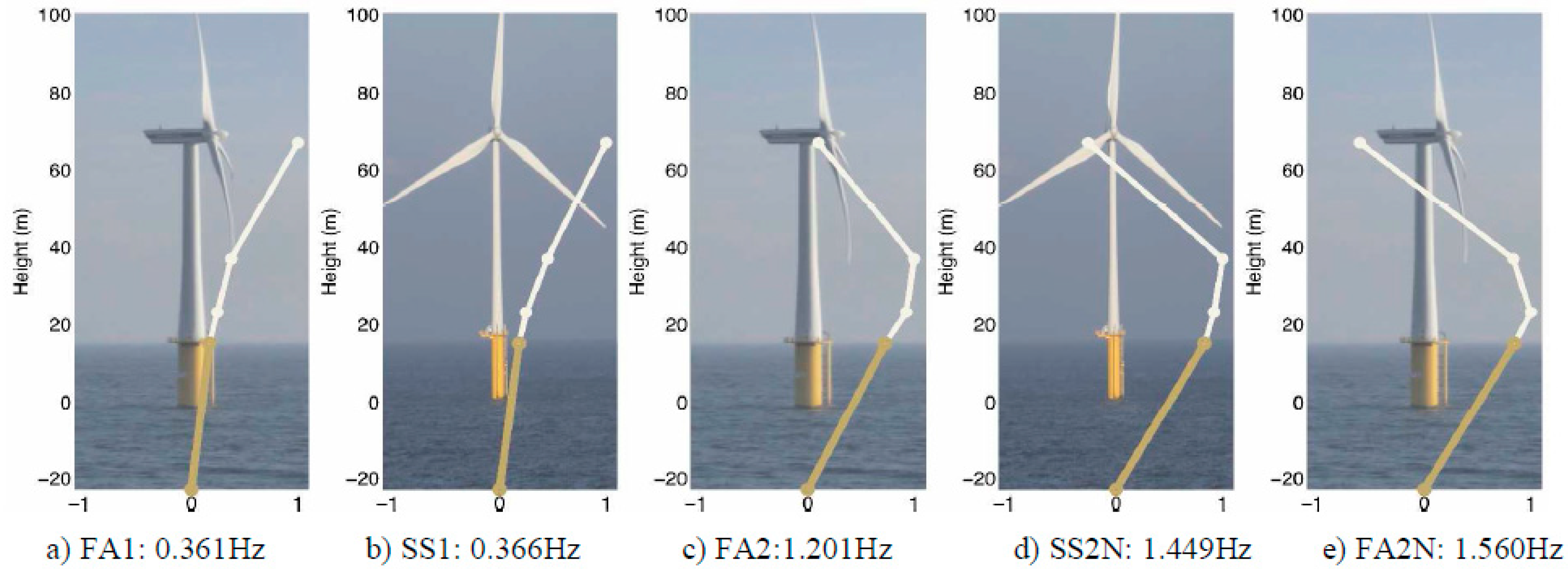
According to the results of some previous intensive studies [7,8,9,10,11,12] on the identification of the physical vibration modes of the tower, foundation system, and the blades of the instrumented OWT, it can be concluded that the most dominant vibration modes of those structures can be detected in a frequency range of 0–2 Hz. For the tower and the foundation system, the most dominant modes are named as follows according to [7]:
- First for-aft bending tower mode (FA1)
- First side-side bending tower mode (SS1)
- Second for-aft bending mode tower component (FA2)
- Second side-side bending mode tower and nacelle component (SS2N)
- Second for-aft bending mode tower and nacelle component (FA2N)
The mode shapes together with the resonance frequency values of those modes are shown in Figure 2. Based on the work done in [8], some other modes related to the blades and the drivetrain can be detected in the frequency band 0–2 Hz. Those modes are the first drivetrain torsional mode (DTT1), the first blade asymmetric flapwise pitch (B1AFP) mode, the first blade asymmetric flapwise yaw (B1AFY) mode, the first blade collective flap (B1CF) mode, and the first blade asymmetric edgewise yaw (B1AEY) mode.
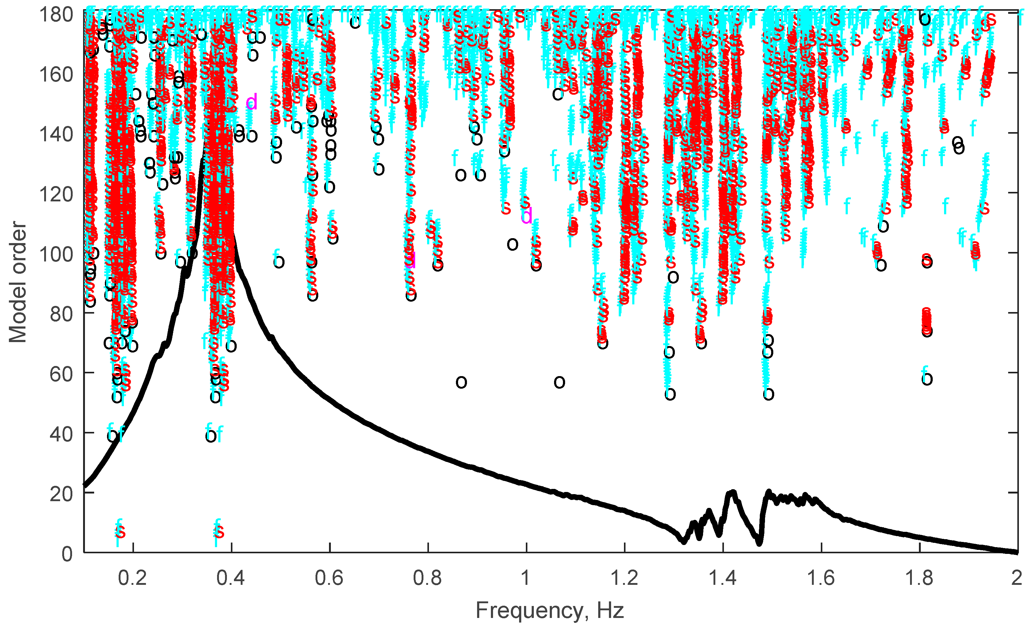
The selected 12 data records are consecutively processed in frequency domain for a frequency band goes up to 2 Hz, and the most dominant in-band modes are estimated and manually tracked based on the frequency values presented in [7,8]. The auto and cross power spectra are estimated using the Correlogram approach [13,14] as it was used in the reference article (i.e., [7]) to estimate the frequency-domain data. The polyreference linear least-squares complex exponential (pLSCE) estimator [15,16] is used to estimate the modes within the selected frequency band, and a stabilization chart is built for each data record to facilitate the selection of the physical vibration modes. The stabilization chart is a very well-known mode selection tool in the modal analysis community. In this chart, the resonance frequencies of the identified poles are visualized for different model orders. The frequency is presented on the x-axis; the vertical axis shows the model order for which the poles are identified. The model order is the polynomial order which the modal parameter estimator uses to fit the measured data. A symbol is associated to each pole corresponding to the degree of the stabilization of the pole in terms of frequency and damping when compared to the analysis at the previous model order. An “o” corresponds to a new identified pole, “f” indicates that the estimated pole is stable in terms of frequency value (i.e., the variation on the frequency value is within for instance 5% when the model order changes), “d” implies that the identified pole is stable in terms of the damping value (i.e., the variation on the damping value is within for instance 10% when the model order changes), “s” corresponds to a pole that is stable in terms of frequency and damping values. In the stabilization chart, the physical modes show relatively consistent behavior when the model order changes. Therefore, they show up in the stabilization chart as vertical lines with a lot of “s” symbol. Figure 3 shows a typical stabilization chart for one of the analyzed data records in the low frequency range. It is found that the dominant tower and blade modes appear consistently at the same locations in the stabilization chart constructed over the different data records. Those modes are selected manually from the stabilization chart based on the values published in [7,8].
In Table 1 and Table 2, the mean value of the resonance frequencies of the tower, blades, and low-frequency drivetrain mode are summarized and compared to the reference values [7,8]. One can see from Table 1 that the dominant tower’s modes are successfully detected except the third mode, i.e., FA2 at 1.20 Hz. This can be explained by the fact that this mode is mostly characterized by a tower motion rather than a nacelle motion (see Figure 2 for the FA2 mode). That is why this mode is not well detectable from signals measured from the drivetrain system.
From Table 1 and Table 2, one can see that the mean value of the resonance frequencies of the global tower modes, the blade modes, and the first torsional drivetrain mode obtained from the signals measured from sensors mounted on the drivetrain agrees very well with the results obtained from signals measured from sensors mounted on the tower itself. The small differences in the values are acceptable, taking into account the following facts: First, the published results in [7] were obtained using datasets of two weeks measured from sensors directly mounted on the tower itself. Second, the ambient conditions were different from the conditions of the drivetrain measurements campaign. Third, the sensors used on the drivetrain measurements campaign are aimed towards higher frequency region.
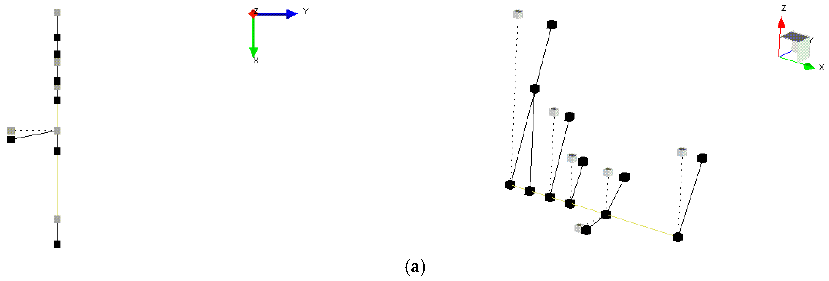
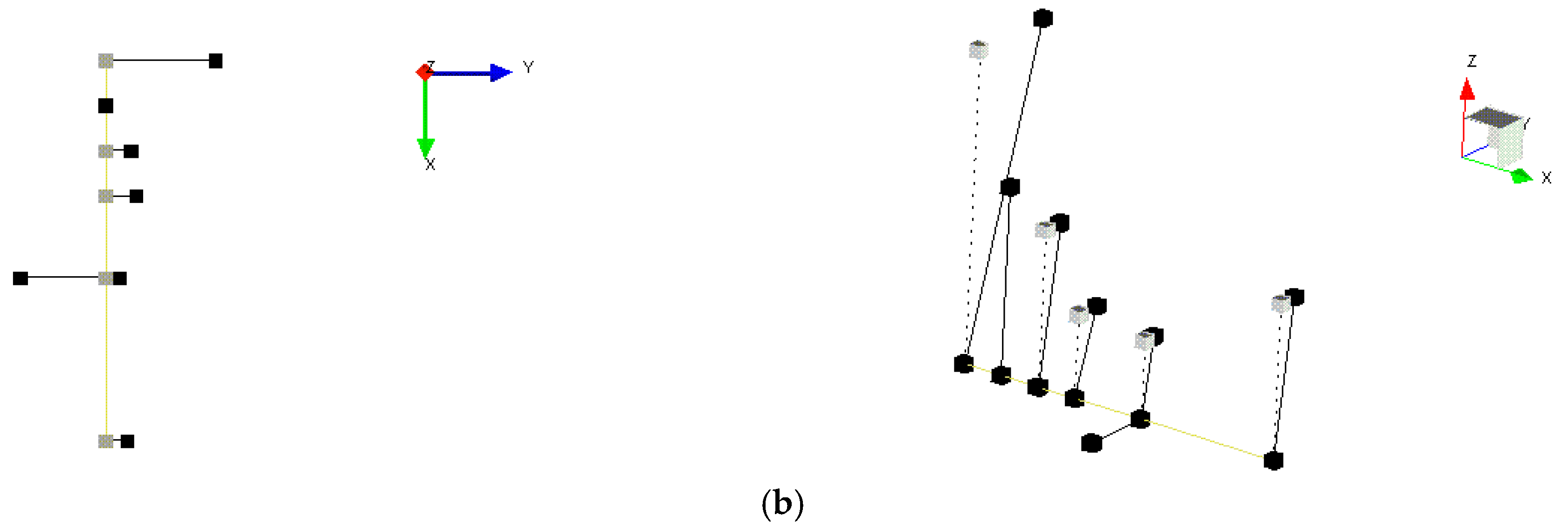
Since no sensors were mounted on the tower, it was not possible to plot the mode shapes of the tower modes. However, in Figure 4 the mode shapes of the drivetrain system at the FA1 and SS1 frequencies are shown. The figure shows 2D and 3D representations for the mode shapes. For the FA1 mode the components of the mode shape in X-direction, which are the dominant ones in comparison to the y-components at that frequency, are plotted. For the SS1 mode, the components in Y-direction, which are the dominant ones in comparison to the x-components at that frequency, are plotted. In that figure, the grey boxes represent the undeformed model, while the black ones represent the deformed model. From these mode shapes, one can see that the movement of the drivetrain system resembles the tower movement where it goes in the for-aft direction (X-dir.) at 0.359 Hz (the tower FA1) and in the side-side direction (Y-dir.) at 0.371 Hz (the tower SS1 mode). The consistency of the obtained results in the low frequency-band with the previously published ones on the same turbine confirms the correctness of the measured data considering that the sensors that have been used on the drivetrain are aimed towards the higher frequency region for dynamic analysis of the drivetrain system.
4. Automatic Tracking of Drivetrain Modes: High Frequency-Band Analysis
In this section, the first results of the short-term automatic tracking of some drivetrain modes will be presented and discussed. The automatic tracking procedure consists of four main steps:
- Loading and reading the time-domain measured acceleration signals;
- Automatic tracking of the modes of interest based on the Modal Assurance Criterion (MAC), frequency value, and damping ratio value.
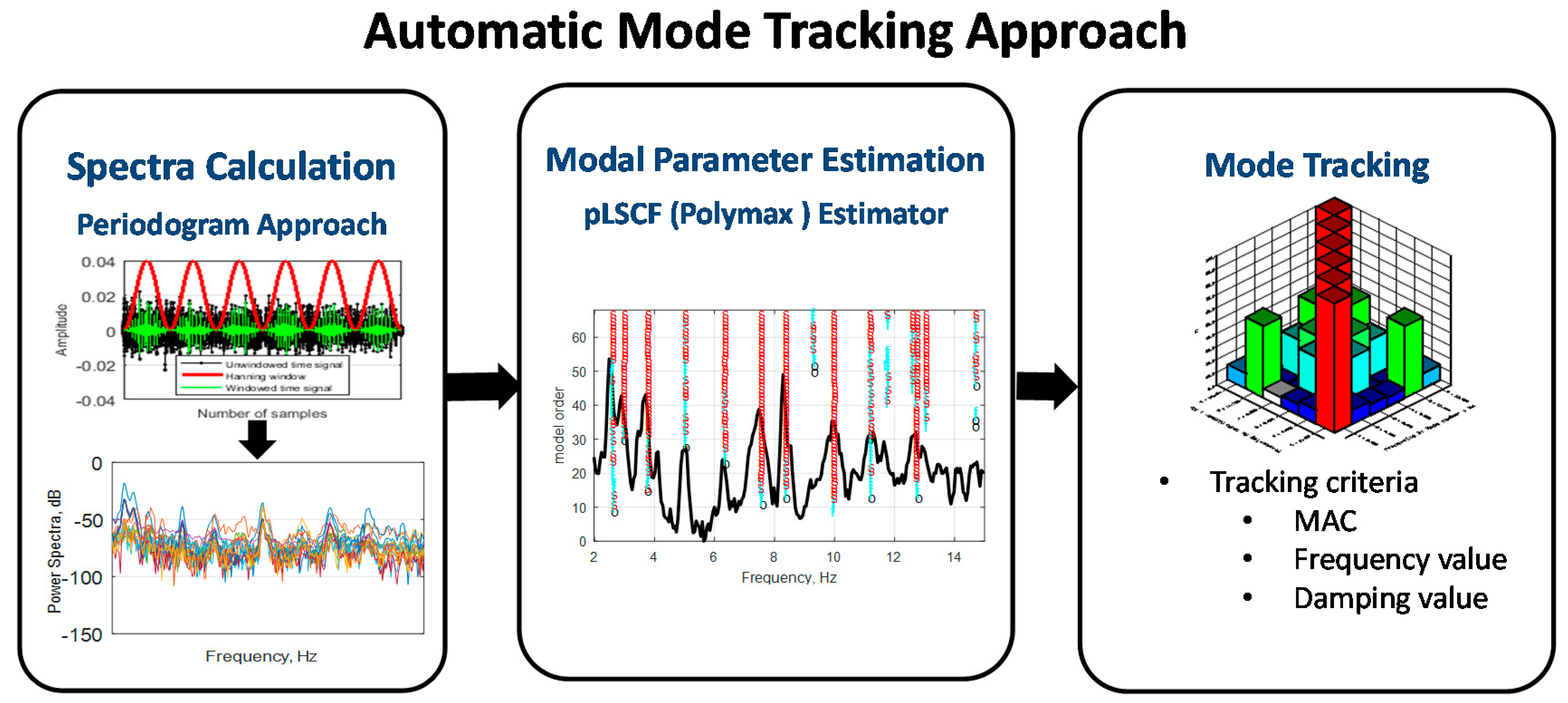
Figure 5 shows a schematic description of the proposed tracking approach. In the following subsections, a brief explanation of the main steps is given.
4.1. The Periodogram Approach
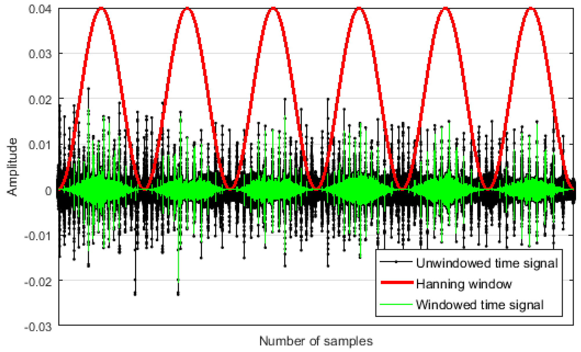
The periodogram approach [17,18] applied to one record of the analyzed dataset is shown in Figure 6. In the Periodogram approach, a time-domain signal record for an output is divided into overlapped sub-records . Then, each sub-record is weighted using a Hanning window to decrease the leakage effects (). Next to that, the discrete Fourier transform (DFT) of each windowed sub-record is calculated and the average of all these sub-record is taken to decrease the random errors. A subset of the output responses is selected to be taken as reference signals to calculate the cross-power spectra. At each frequency line , a full power spectra matrix with dimensions will be estimated with the number of the measured outputs and the number of the channels taken as reference. The following Equations (1) and (2) show how the averaged auto and cross power spectra are estimated:
where is the circular frequency in , stands for the complex conjugate of a complex number, and . An example of the obtained power spectra is shown in Figure 7.
4.2. The Polyreference Least-Squares Complex Frequency-Domain (pLSCF) Estimator
The pLSCF estimator [19,20], which is normally applied to the frequency response functions (FRFs) data, can be applied to the output power spectra in case of OMA under the assumption of white noise input. In the pLSCF method, the following so-called right matrix fraction description model is assumed to represent the measured power spectra matrix of the outputs:
where are the numerator matrix polynomial coefficients, are the denominator matrix polynomial coefficients, is the model order, is the number of measured outputs, and is the number of response DOFs taken as references. The pLSCF estimator uses a discrete time frequency domain model (z-domain model) with ( is the circular frequency in and is the sampling time).
Equation (3) can be written for all the values of the frequency axis of the power spectra data. The unknown model coefficients and are then found as the least squares solution of these equations. Once the denominator coefficients are determined, the poles and the modal operational reference factors are retrieved as the eigenvalues and eigenvectors of their companion matrix. An order right matrix-fraction model yields poles. For a displacement output quantity, the full power spectrum can be written as a function of the modal parameters (pole , modal operational reference factors , mode shapes ) as [21,22]:
with the number of estimated modes, and are the lower and upper residual terms to model the effects of the out-of-band modes. After the poles and the operational reference factors are estimated from Equation (3), the mode shapes and the lower and upper residual terms are the only unknowns in Equation (4). They are readily obtained by solving Equation (4) in a linear least-squares sense. The goal of OMA is to identify the right-hand side terms of Equation (4) based on measured output data pre-processed into output spectra (). From the pole value , the damped resonance frequency and the damping ratio are calculated.
4.3. Automatic Mode Tracking Criteria
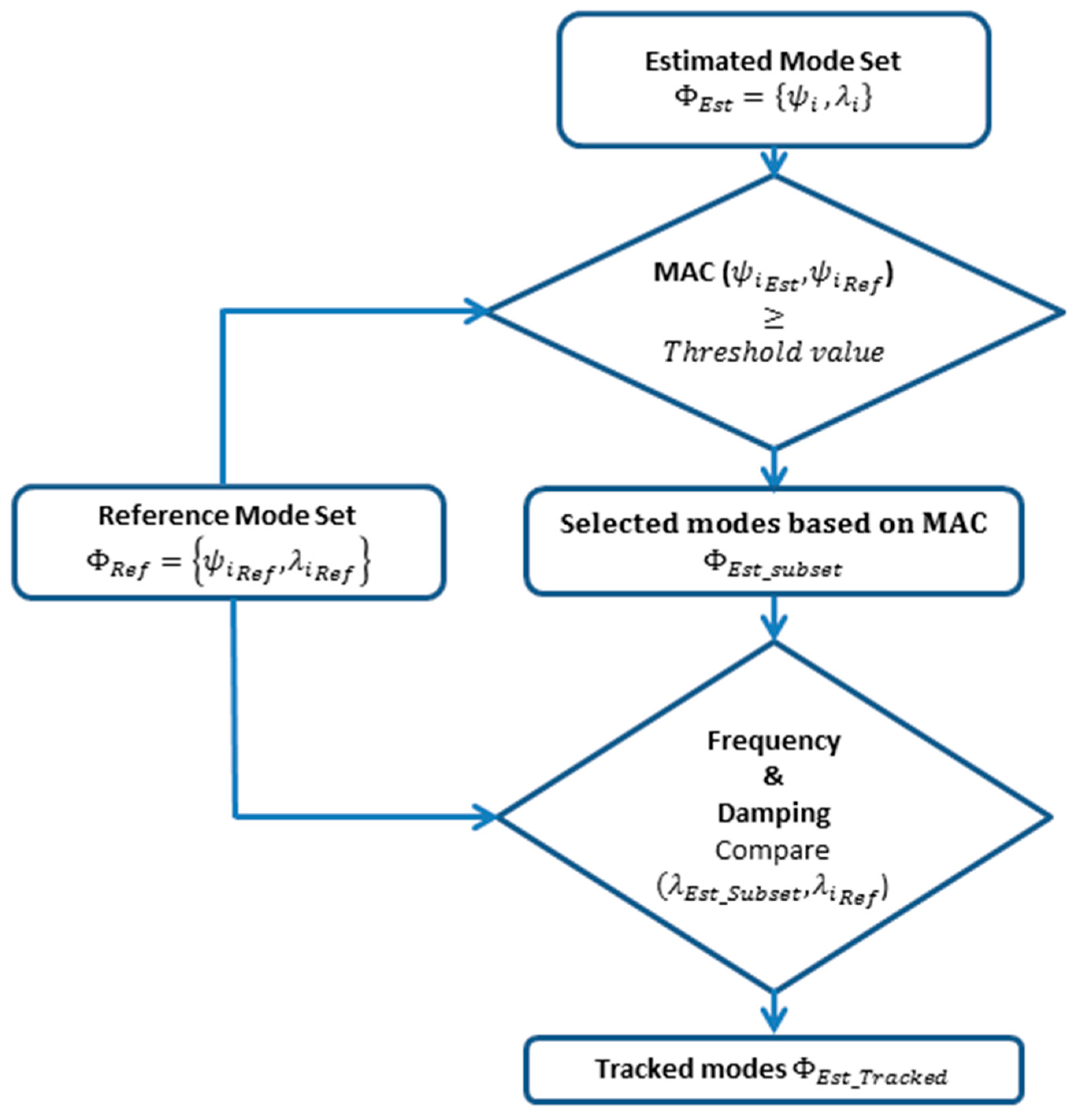
In this step, the modal parameters estimated from the pLSCF step for a data record are compared to the modal parameters of the reference modes set. Figure 8 shows a flowchart that represents the criteria that have been used for the mode tracking. A comparison between the estimated modes and the reference mode set is done in terms of the Modal Assurance Criterion (MAC) and the pole value. The MAC value measures how coherent is the estimated mode with respect to the reference one in terms of the mode shapes, while the pole value indicates how close is the estimated mode to the reference one in terms of frequency and damping values. First, a subset of the estimated modes that show a MAC value with respect to the reference mode higher than a user defined threshold value (e.g., ≥60%) are selected. Then, the closest mode to the reference one in terms of frequency and damping values is selected from this subset.
5. Discussion on the First Results of the Automatic Tracking of the Drivetrain Modes
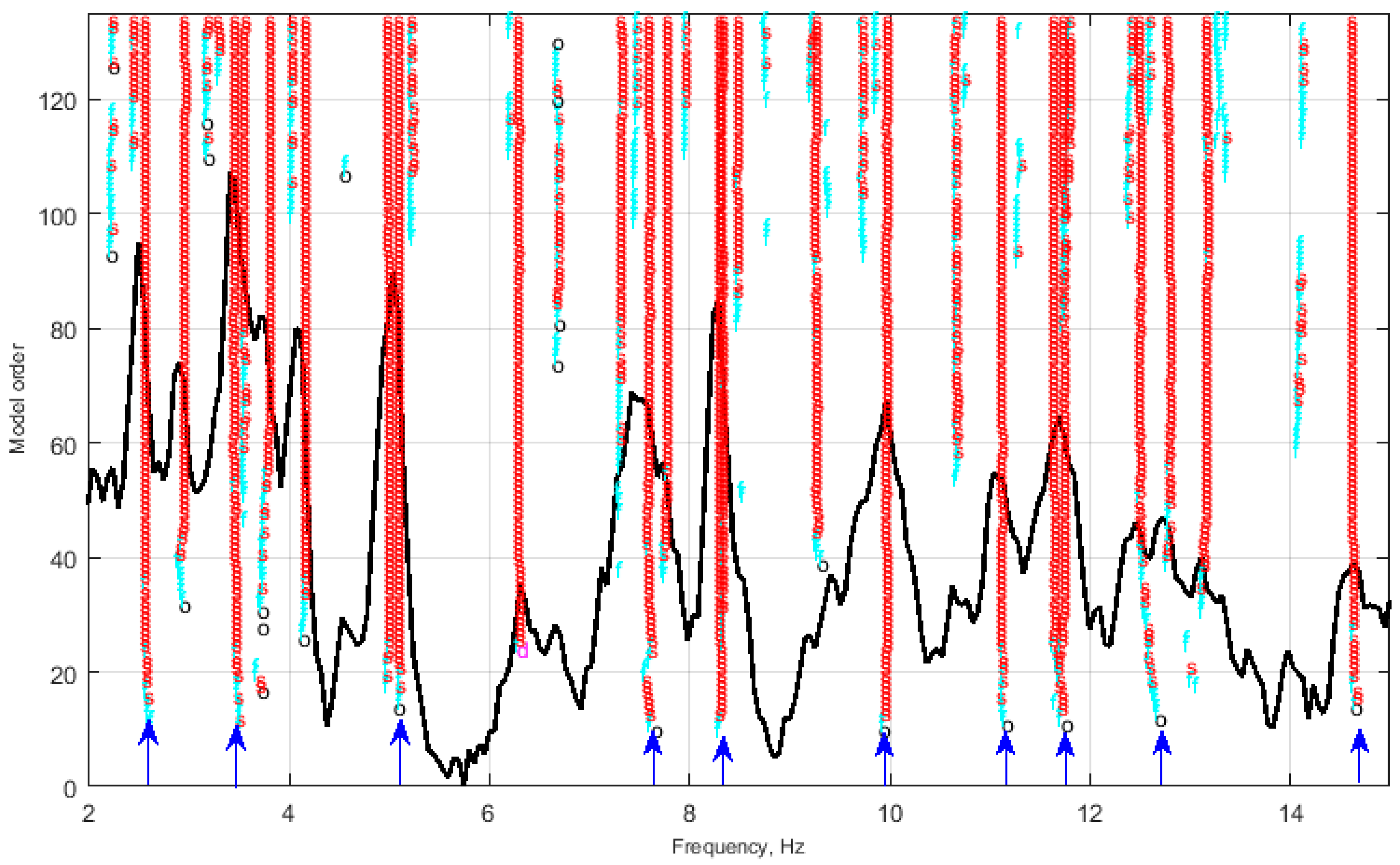
This paper investigates the turbine modal behavior while it is not producing energy. This specific operating condition will have an impact on the modal behavior observed in the drivetrain, since the teeth can be out of contact during these conditions; whereas this is necessarily the case for nominal power production [23]. Moreover, the damping properties of the wind turbine will change according to the operating conditions [24]. The different steps described in Section 4 are implemented in MATLAB (Version 2016a, MathWorks, Eindhoven, Netherlands) , and they are applied to the different time-domain data records. The modal parameter estimation is done in a frequency band goes from 2 Hz to 15 Hz. In this frequency band, the pLSCF modal parameter estimator finds many modes that are related to the drivetrain dynamics. Figure 9 shows a typical stabilization chart constructed by the pLSCF estimator when applied to the power spectra matrix of the first data record. It can be seen from that figure that there are many modes in the analysis band. Some of these modes show up even if a low model order is used (indicated by the blue arrows), while some other modes are stabilized at a relatively higher model order. The model order is the polynomial order that the pLSCF estimator uses to fit Equation (3) to the measured data (see Section 4.2 for more details). For those modes that are detected at low model order, they are considered as the most dominant and physical modes for the structure under test since their observability is relatively high (i.e., can be detected at very low model order). Therefore, since a detailed knowledge about the specifics of the drivetrain itself and its vibration modes is not available, we selected those 10 most dominant modes, i.e., the ones indicated by the blue arrows in Figure 9, to be tracked. The mode shapes and the pole values of those 10 dominant modes estimated from the first data record are taken as reference modes set. The mode shapes of those 10 modes are represented in Figure 10.
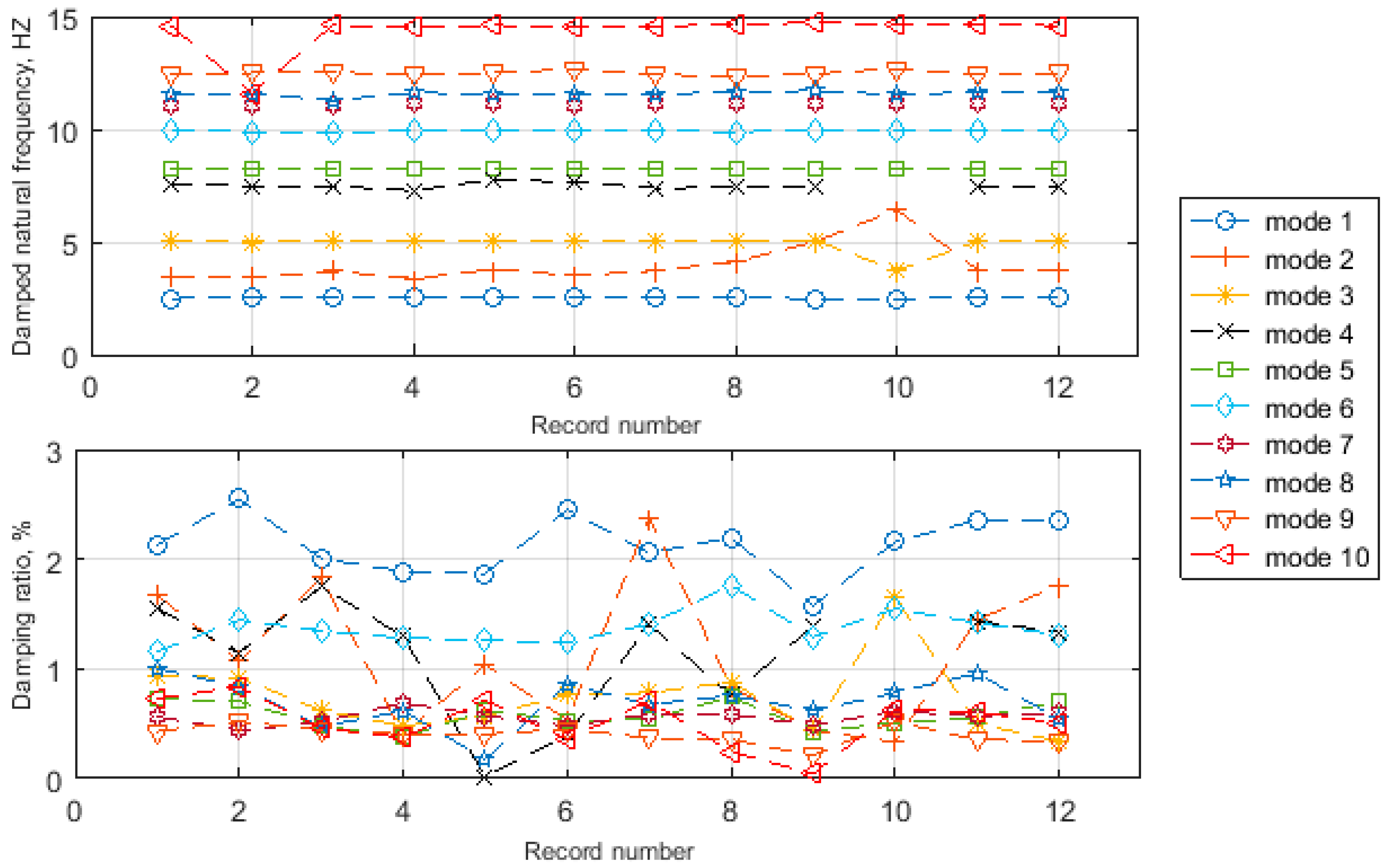
Figure 11 represents the evolution of the natural frequencies and the damping ratios of the 10 most dominant drivetrain modes identified in the analysis band, while Figure 12 represents the evolution of the MAC calculated between the estimated mode shapes of the 10 most dominant modes and the reference ones over the tracking period. It can be seen that the frequency values are more consistent in comparison to the damping estimates, which is normal since the damping is highly affected by the ambient conditions (e.g., wind speed). The effect of the ambient conditions on the consistency of the damping estimates can be explained by the fact that the wind turbine is a multi-physical machine with significant interaction between their subcomponents, and for the instrumented wind turbine the rotor is directly connected to the gearbox. Therefore, it is normal that the damping estimates for the drivetrain modes will be affected by the external ambient conditions. This can be also noted from the boxplots of the frequencies and damping ratios shown in Figure 13. This figure illustrates one box and whisker plot per frequency and damping value of each tracked mode. The results in this figure show that, for all the modes, the resonance frequency values show a good level of consistency over the different data blocks except for the second mode.
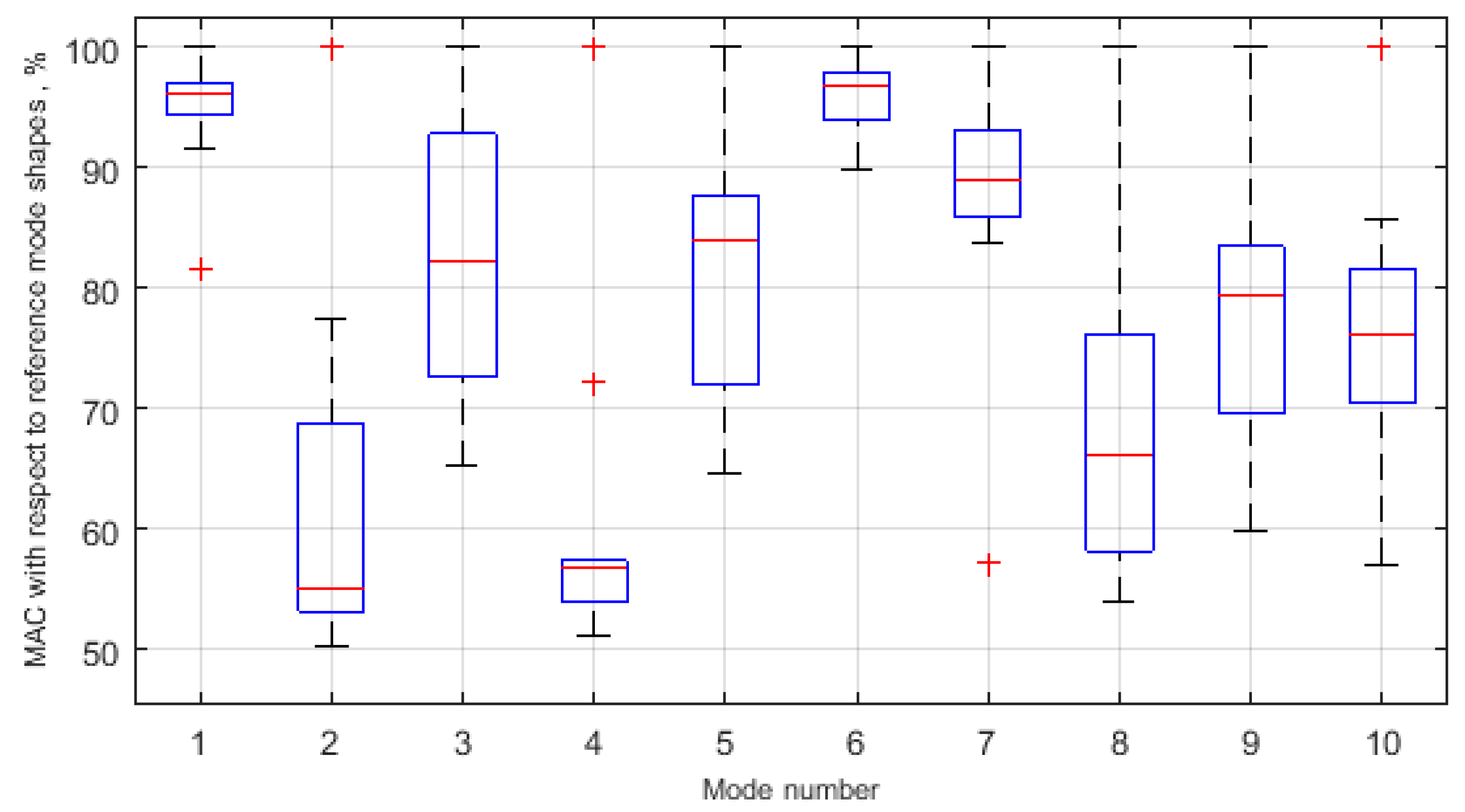
In Figure 11, it can be seen that it could happen that the second and the third modes are crossing each other. In terms of damping value, the second and the fourth modes have the highest level of scatter in comparison to the other modes. In terms of the mode shapes, one can see from Figure 12 and Figure 14 that most of the identified modes show a consistent behavior in term of the mode shapes where the median of the MAC value is above 60%. The second and the fourth modes show the lowest MAC over the tracking period in comparison with the other modes, and this agrees with their behavior in terms of frequency and damping (see Figure 13).
This level of the consistency of the results over the tracking period (i.e., the 12 different processed data records) shows the repeatability of the analysis and underpins the applicability of the measurements and the modal estimation approach for the characterizing drivetrain model behavior.
In the case where the turbine is in operating conditions, the presence of the rotating components and their corresponding harmonics force contributions that do not comply with the OMA assumption (i.e., the input forces are white noise) will make the modal parameter estimation process difficult. In this case, special care must be taken to avoid mistaken harmonic components for true structural modes. Harmonics removal techniques [25] can be used to clean the data from the harmonic components before doing the modal parameter estimation step. Therefore, the automatic mode tracking approach described in Section 4 can be used when the wind turbine is in operating conditions provided that a harmonics-removing technique is used in advance to separate the true structural modes from the harmonic components. The analysis in this paper is focused on wind turbines in a standstill condition to ensure that the harmonics do not dominate the frequency spectrum and accurate estimates for the modal parameters of the drive train system will be obtained. These modal parameter estimates can be used as reference values when analyzing the wind turbine in operating conditions.
6. Conclusions
The modal behavior of an OWT is investigated while the OWT was in a standstill condition. The investigation is done by performing a short-term tracking of the modal parameters of the different components of the turbine, e.g., tower, blades, and drivetrain system. The signals used to estimate the modal parameters are 17 acceleration signals acquired from 5 tri-axial and 2 uni-axial accelerometers mounted on the drivetrain system (i.e., gearbox & generator) of the turbine. The good agreement between the obtained results in the low frequency band (mainly the tower and blade modal parameters) and the published ones confirms the validity of the measurements considering that the sensors that have been used on the drivetrain are aimed towards higher frequency region for dynamic analysis of the drivetrain system. An automatic tracking approach has been introduced to track some of the drivetrain modes in the high frequency bands. This tracking approach is an initial step towards the full dynamic characterization of the modal behavior of the drivetrain system. The results obtained from this tracking approach show the repeatability of the analysis and confirm the applicability of the used technique for characterizing the drivetrain modal behavior in a standstill condition. Further investigations for the modal behavior of the drivetrain will be continued, and tracking modes in operational condition will be done.
Acknowledgments
The authors would like to acknowledge the VLAIO SBO HYMOP and Proteus Project, as well as the farm owner and the original equipment manufacturer OEM for facilitating the measurement campaign.
Author Contributions
Jan Helsen and Christof Devriendt designed and performed the experiments; Mahmoud El-kafafy analyzed the data and wrote the paper; Patrick Guillaume conceived the data analysis procedure and tools.
Conflicts of Interest
The authors declare no conflict of interest.
References
- Mann, J. Wind field simulation. Probab. Eng. Mech. 1998, 13, 269–282. [Google Scholar] [CrossRef]
- Peeters, J.; Vandepitte, D.; Sas, P. Analysis of internal drive train dynamics in a wind turbine. Wind Energy 2006, 9, 141–161. [Google Scholar] [CrossRef]
- Peeters, J. Simulation of Dynamic Drive Train Loads in a Wind Turbine. Ph.D. Thesis, Katholieke Universiteit Leuven, Leuven (Heverlee), Belgium, 2006. [Google Scholar]
- Veers, P.S. Three-Dimensional Wind Simulation; SAND-88-0152C, CONF-890102-9-ON: DE89003171; Sandia: Albuquerque, New Mexico 87185; Livermore, CA, USA, 1988.
- Goris, S.; Vanhollebeke, F.; Ribbentrop, A.; Markiewicz, M.; Schneider, L.; Wartzack, S.; Hendrickx, W.; Desmet, W. A validated virtual prototyping approach for avoiding wind turbine tonality. In Proceedings of the Wind Turbine Noise, Denver, CO, USA, 28–30 August 2013. [Google Scholar]
- Helsen, J. The Dynamics of High Power Density Gearboxes with Special Focus on the Wind Turbine Application. Ph.D. Thesis, Katholieke Universiteit Leuven, Leuven (Heverlee), Belgium, 2012. [Google Scholar]
- Devriendt, C.; Weijtjens, W.; El-Kafafy, M.; De Sitter, G. Monitoring resonant frequencies and damping values of an offshore wind turbine in parked conditions. IET Renew. Power Gener. 2014, 8, 433–441. [Google Scholar] [CrossRef]
- Shirzadeh, R.; Weijtjens, W.; Guillaume, P.; Devriendt, C. The dynamics of an offshore wind turbine in parked conditions: A comparison between simulations and measurements. Wind Energy 2015, 18, 1685–1702. [Google Scholar] [CrossRef]
- Devriendt, C.; El-Kafafy, M.; De Sitter, G.; Cunha, A.; Guillaume, P. Long-term dynamic monitoring of an offshore wind turbine. In Proceedings of the IMAC-XXXI, Garden Grove, CA, USA, 11–14 February 2013. [Google Scholar]
- Devriendt, C.; El-Kafafy, M.; De Sitter, G.; Guillaume, P. Estimating damping of an offshore wind turbine using an overspeed stop and ambient excitation. In Proceedings of the 15th International Conference on Experimental Mechanices ICEM15, Porto, Portugal, 22–27 July 2012. [Google Scholar]
- Devriendt, C.; El-Kafafy, M.; De Sitter, G.; Jordaens, P.J.; Guillaume, P. Continuous dynamic monitoring of an offshore wind turbine on a monopile foundation. In Proceedings of the ISMA2012, Leuven, Belgium, 17–19 September 2012. [Google Scholar]
- El-Kafafy, M.; Devriendt, C.; Weijtjens, W.; De Sitter, G.; Guillaume, P. Evaluating different automated operational modal analysis techniques for the continuous monitoring of offshore wind turbines. In Proceedings of the International Modal Analysis Conference IMAC XXXII, Orlando, FL, USA, 3–6 February 2014. [Google Scholar]
- Bendat, J.; Piersol, A. Random Data: Analysis and Meaurment Procedures; John Wiley & Sons: New York, NY, USA, 1971. [Google Scholar]
- Blackman, R.B.; Tukey, J.W. The measurement of power spectra from the point of view of communications engineering—Part I. Bell Syst. Tech. J. 1958, 37, 185–282. [Google Scholar] [CrossRef]
- Brown, D.L.; Allemang, R.J.; Zimmerman, R.; Mergeay, M. Parameter estimation techniques for modal analysis. SAE Trans. Paper Ser. 1979, 828–846. [Google Scholar] [CrossRef]
- Vold, H. Numerically robust frequency domain modal parameter estimation. Sound Vib. 1990, 24, 38–40. [Google Scholar]
- Marple, S.L. Digital Spectral Analysis: With Applications; Prentice-Hall, Inc.: Upper Saddle River, NJ, USA, 1986. [Google Scholar]
- Welch, P.D. The use of fast fourier transform for the estimation of power spectra: A method based on time averaging short modified periodograms. IEEE Trans. Audio Electroacoust. 1967, 15, 70–73. [Google Scholar] [CrossRef]
- Guillaume, P.; Verboven, P.; Vanlanduit, S.; Van der Auweraer, H.; Peeters, B. A poly-reference implementation of the least-squares complex frequency domain-estimator. In Proceedings of the 21th International Modal Analysis Conference (IMAC), Kissimmee, FL, USA, 3–6 February 2003. [Google Scholar]
- Peeters, B.; Van der Auweraer, H.; Guillaume, P.; Leuridan, J. The PolyMAX frequency-domain method: A new standard for modal parameter estimation? Shock Vib. 2004, 11, 395–409. [Google Scholar] [CrossRef]
- Peeters, B.; Van der Auweraer, H.; Vanhollebeke, F.; Guillaume, P. Operational modal analysis for estimating the dynamic properties of a stadium structure during a football game. Shock Vib. 2007, 14, 283–303. [Google Scholar] [CrossRef]
- Hermans, L.; Van der Auweraer, H. Modal testing and analysis of structures under opertional conditions: Industrial Applications. Mech. Syst. Signal Proc. 1999, 13, 193–216. [Google Scholar] [CrossRef]
- Vanhollebeke, F.; Peeters, P.; Helsen, J.; Di Lorenzo, E.; Manzato, S.; Peeters, J.; Vandepitte, D.; Desmet, W. Large Scale Validation of a Flexible Multibody Wind Turbine Gearbox Model. J. Comput. Nonlinear Dyn. 2015, 10, 041006. [Google Scholar] [CrossRef]
- Weijtjens, W.; Shirzadeh, R.; De Sitter, G.; Devriendt, C. Classifying resonant frequencies and damping values of an offshore wind turbine on a monopole foundation for different operational conditions. In Proceedings of the EWEA, Copenhagen, Denmark, 10–13 March 2014. [Google Scholar]
- Manzato, S.; Mooccia, D.; Peeters, B.; Janssens, K.; White, J. A review of harmonic removal methods for improved operational modal analysis of wind turbines. In Proceedings of the ISMA2012, Leuven, Belgium, 17–19 September 2012. [Google Scholar]
Figure 1.
(a) A layout of the drivetrain; (b) the structure of the instrumented wind turbine; (c) Measurement locations on the drivetrain unit with zoom in on the sensor locations; (d) a simple geometry representing the locations of the tri-axial sensors (indicated by three axes) and the uni-axial sensors (indicated by one axis) at the different stages of the drivetrain unit (Black boxes: the sensors on the gearbox unit. Blue box: sensor on the generator unit.).
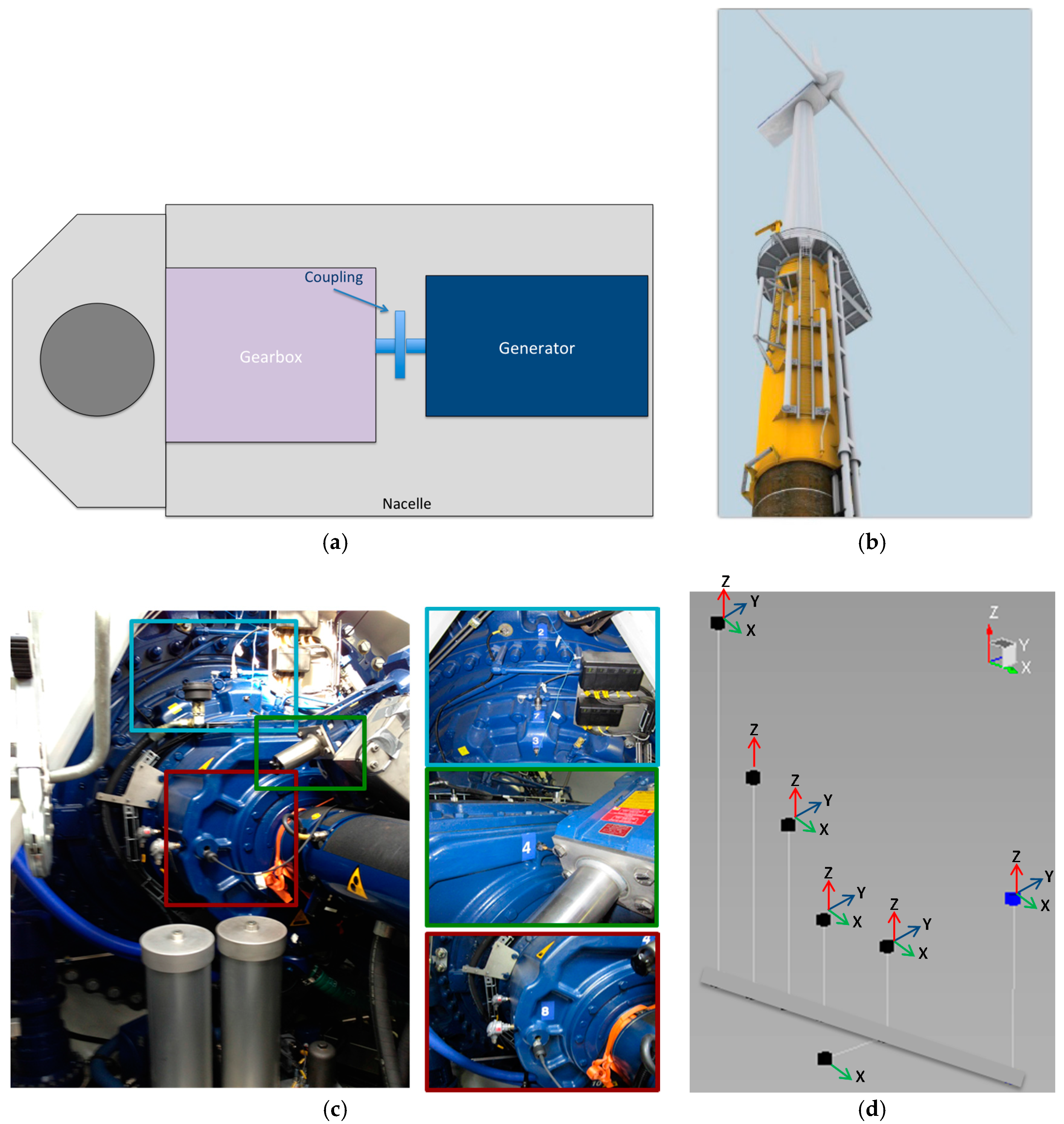
Figure 2.
Low frequency band analysis: Dominant modes of the tower of the instrumented offshore wind turbine (OWT) [7].
Figure 2.
Low frequency band analysis: Dominant modes of the tower of the instrumented offshore wind turbine (OWT) [7].

Figure 3.
A typical stabilization chart constructed by the polyreference linear least-squares complex exponential (pLSCE) estimator in the low frequency band.
Figure 3.
A typical stabilization chart constructed by the polyreference linear least-squares complex exponential (pLSCE) estimator in the low frequency band.

Figure 4.
(a) The drivetrain mode shape at the tower FA1 frequency: 0.359 Hz. (b) The drivetrain mode shape at the tower SS1 frequency: 0.369 Hz. (Y: Side-Side direction X: For-Aft direction Grey boxes: undeformed model Black boxes: deformed model).
Figure 4.
(a) The drivetrain mode shape at the tower FA1 frequency: 0.359 Hz. (b) The drivetrain mode shape at the tower SS1 frequency: 0.369 Hz. (Y: Side-Side direction X: For-Aft direction Grey boxes: undeformed model Black boxes: deformed model).


Figure 5.
The different steps of the automatic tracking procedure of the drivetrain modes.

Figure 6.
Periodogram approach applied to one data record.

Figure 7.
Obtained averaged cross power spectra between all the outputs and the first reference.
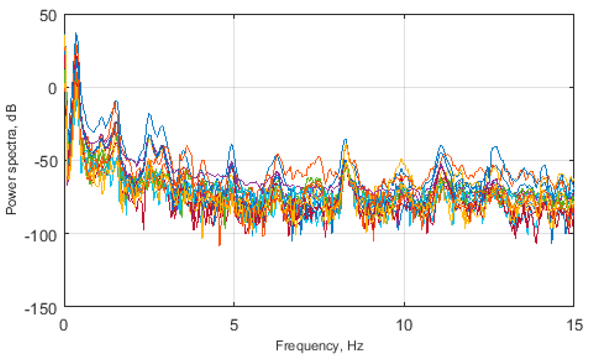
Figure 8.
Drivetrain modes tracking criteria.

Figure 9.
Stabilization chart constructed by the pLSCF estimator when applied to the first data record.
Figure 9.
Stabilization chart constructed by the pLSCF estimator when applied to the first data record.

Figure 10.
The mode shapes of the 10 tracked drivetrain modes.
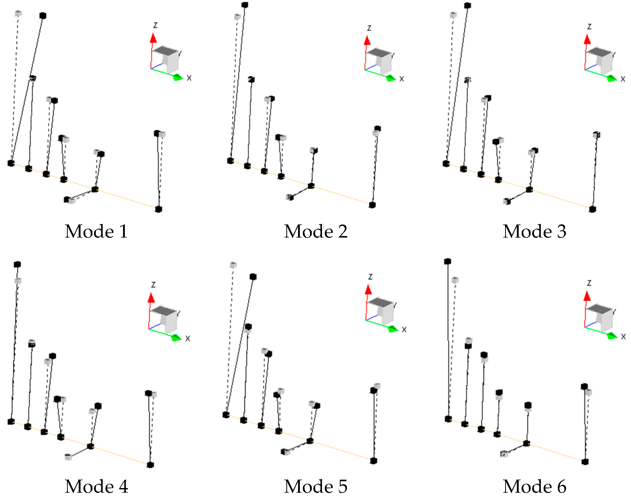
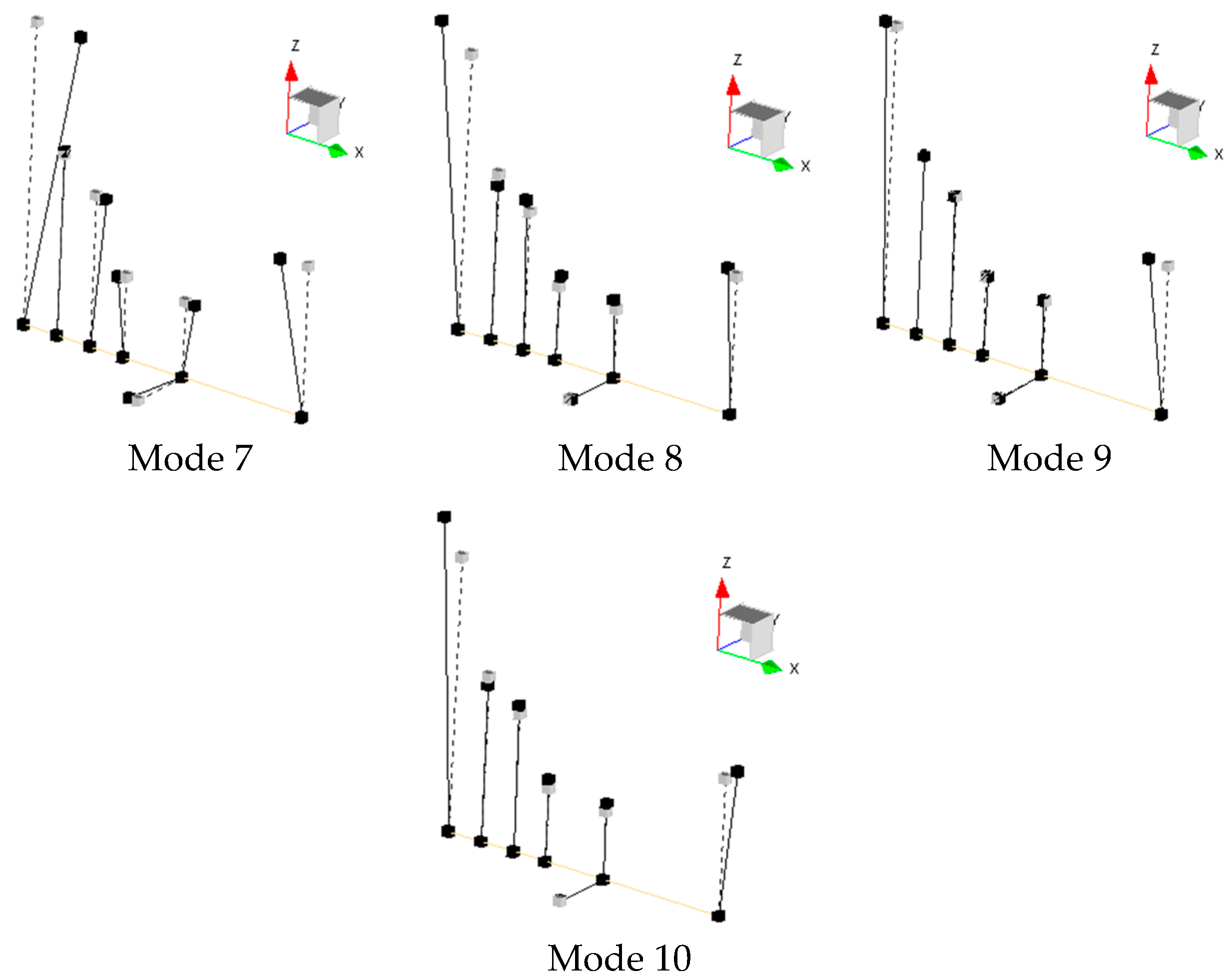
Figure 11.
Evolution of the frequencies (top) and damping ratios (bottom) of the 10 most dominant drivetrain modes during the tracking period.
Figure 11.
Evolution of the frequencies (top) and damping ratios (bottom) of the 10 most dominant drivetrain modes during the tracking period.

Figure 12.
Evolution of the MAC value calculated between the 10 most dominant drivetrain modes and the reference mode shapes during the tracking period.
Figure 12.
Evolution of the MAC value calculated between the 10 most dominant drivetrain modes and the reference mode shapes during the tracking period.
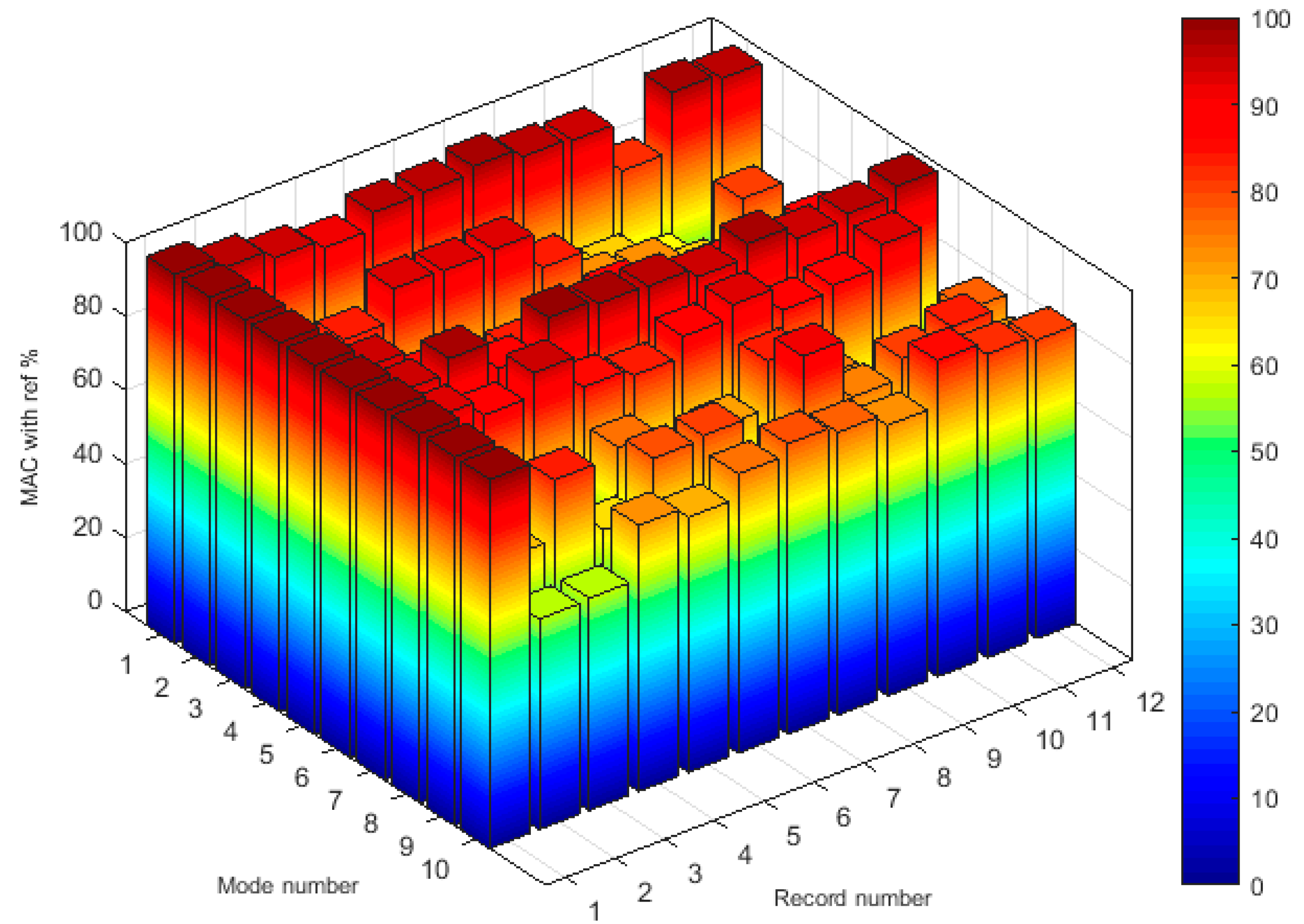
Figure 13.
Boxplots of the frequencies (left) and damping ratios (right) of the 10 most dominant drivetrain modes over the tracking period: On each box, the central mark is the median, the edges of the box are the 25th and 75th percentiles, the whiskers extend to the most extreme values that were not considered as outliers and the outliers are plotted individually using the “+” symbol.
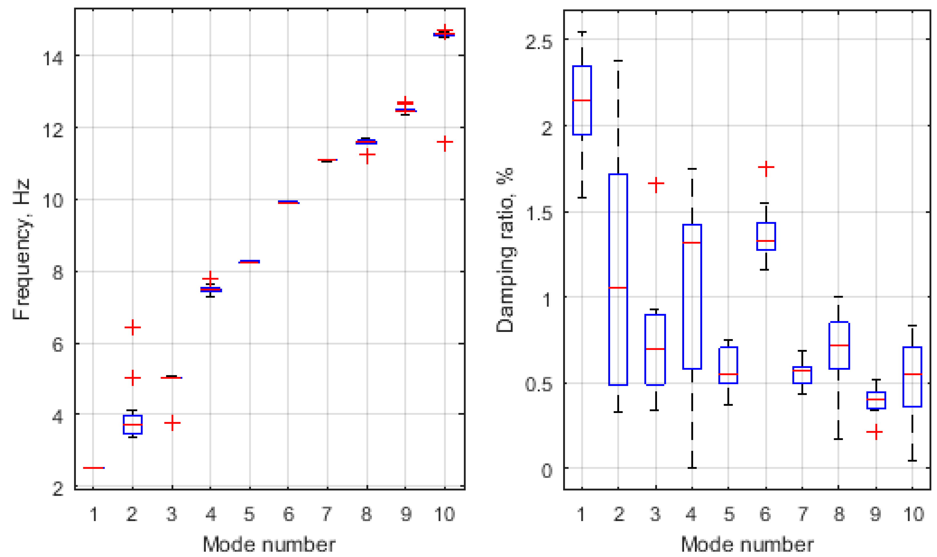
Figure 14.
Boxplots of the MAC value calculated between the 10 most dominant drivetrain modes and the reference mode shapes over the tracking period: On each box, the central mark is the median, the edges of the box are the 25th and 75th percentiles, the whiskers extend to the most extreme values that were not considered as outliers and the outliers are plotted individually using the “+” symbol.

Table 1.
Results of the short-term manual tracking of the low frequency-band (0–2 Hz) modes (Tower’s modes).
Table 1.
Results of the short-term manual tracking of the low frequency-band (0–2 Hz) modes (Tower’s modes).
| Mode | Mean Value of the Resonance Frequencies of the Global Tower Modes [Hz] | |
| Estimated based on signals from sensors on the drivetrain | Estimated based on signals from sensors on the tower [7] | |
| FA1 | 0.359 | 0.361 |
| SS1 | 0.369 | 0.366 |
| SS2N | 1.460 | 1.449 |
| FA2N | 1.563 | 1.560 |
Table 2.
Results of the short-term manual tracking of the low frequency-band (0–2 Hz) modes (Blade modes and first torsional mode of the drivetrain system).
Table 2.
Results of the short-term manual tracking of the low frequency-band (0–2 Hz) modes (Blade modes and first torsional mode of the drivetrain system).
| Mode | Mean Value of the Resonance Frequencies of Blade and Drivetrain Modes [Hz] | |
| Estimated based on signals from sensors on the drivetrain | Estimated based on signals from sensors on the tower [8] | |
| B1AEY | 1.355 | 1.357 |
| B1AFP | 0.642 | 0.667 |
| B1AFY | 0.758 | 0.753 |
| B1CF | 1.141 | 1.152 |
| DTT1 | 1.071 | 1.071 |
© 2017 by the authors. Licensee MDPI, Basel, Switzerland. This article is an open access article distributed under the terms and conditions of the Creative Commons Attribution (CC BY) license (http://creativecommons.org/licenses/by/4.0/).
Share and Cite
MDPI and ACS Style
El-Kafafy, M.; Devriendt, C.; Guillaume, P.; Helsen, J. Automatic Tracking of the Modal Parameters of an Offshore Wind Turbine Drivetrain System. Energies 2017, 10, 574. https://doi.org/10.3390/en10040574
AMA Style
El-Kafafy M, Devriendt C, Guillaume P, Helsen J. Automatic Tracking of the Modal Parameters of an Offshore Wind Turbine Drivetrain System. Energies. 2017; 10(4):574. https://doi.org/10.3390/en10040574
Chicago/Turabian StyleEl-Kafafy, Mahmoud, Christof Devriendt, Patrick Guillaume, and Jan Helsen. 2017. "Automatic Tracking of the Modal Parameters of an Offshore Wind Turbine Drivetrain System" Energies 10, no. 4: 574. https://doi.org/10.3390/en10040574
Note that from the first issue of 2016, this journal uses article numbers instead of page numbers. See further details here.