
H∞ Repetitive Control Based on Active Damping with Reduced Computation Delay for LCL-Type Grid-Connected Inverters

Key Laboratory of Smart Grid of Ministry of Education, Tianjin University, No. 92 Weijin Road, Nankai District, Tianjin 300072, China
*
Author to whom correspondence should be addressed.
Energies 2017, 10(5), 586; https://doi.org/10.3390/en10050586
Submission received: 21 February 2017
/
Revised: 20 April 2017
/
Accepted: 20 April 2017
/
Published: 25 April 2017
(This article belongs to the Section F: Electrical Engineering)
Abstract
:In the paper, the H∞ repetitive current control scheme based on active damping along with the design method is proposed for three-phase grid-connected inverters with inductor-capacitor-inductor (LCL) filters. The control scheme aims to reduce the harmonic distortion of the output currents and achieve better efficiency. The design method introduces capacitor-current-feedback active damping into the H∞ controller design process by proposing an equivalent controlled plant. Additionally, based on the discrete model of the controlled plant with variable computation delay, the algebraic expression of the stable region for the feedback coefficient and the computation delay is obtained to avoid system instability caused by the digital control delay. Finally, the stability criterion is proposed to evaluate the stability of the discrete control system with the H∞ repetitive current control scheme. The theoretical analysis and experimental results prove that the control scheme presented in this paper not only can reject the harmonics of output currents, but is robust under the variation of the grid-impedance.
1. Introduction
As the application of distributed generation is rapidly growing, the voltage-source-inverter (VSI) is commonly used as the interface between a distributed generator and the grid. While the VSI always works as the current source when it is connected to the grid, the harmonic distortion of the output current is a major issue as it can cause extra power loss and resonance of the grid. Therefore, the current control scheme of VSI should not only control the power output, but restrain the current harmonics injection.
LCL filters have been widely adopted in VSIs to attenuate the switching frequency harmonics [1]. However, the resonance introduced by the LCL filter requires extra damping to guarantee the stability of the current control system. One common solution is passive damping, which adds extra resistance into the filter [2]. This method increases the power loss of the LCL filter. Therefore, the active damping method has been proposed in references [3,4]. Without introducing additional resistance, the active damping strategy feeds back the state variable signal of the LCL filter into the control system to damp the filter resonance. Active damping avoids the power loss caused by additional resistance and provides more flexibility in adjusting the performance of the inverters. Several active damping methods have been proposed in recent years. Different state variables such as capacitor current [5], capacitor voltage [6], or inductor current [4,7,8] have been used to damp the filter resonance. These methods have their advantages and disadvantages in practice. The advantage of the capacitor-current-feedback active damping is that the damping effect can be achieved via a simple proportional control of the feedback signal. Compared with other methods which introduce software filters [4,7,8] or other control algorithms [6] to realize the active damping, the adoption of proportional capacitor-current-feedback can reduce the complexity of the control system design and analysis. However, when capacitor-current-feedback is adopted to realize active damping in a digital control system, the computation delay and pulse-width-modulation (PWM) can affect the stability of the system [9,10]. As suggested in reference [9], if the computation delay is one sampling period, a critical resonant frequency exists and is equal to 1/6 sampling frequency (denoted as fs). Only when the resonant frequency of the LCL filter is less than the critical resonant frequency, can the feedback of the capacitor-current damp the resonance. The research in reference [10] shows that an increase of the proportional coefficient can increase the equivalent resonant frequency of the damped filter, which may exceed the critical resonant frequency and destabilize the system. Therefore, two basic ideas have been proposed to extend the valid region of capacitor-current-feedback active damping. One is reducing the computation delay. This method was presented in reference [10] based on virtual impedance theory when a proportional-resonant (PR) controller was adopted. However, only the reduction of the computation delay in the capacitor-current feedback loop was discussed. The relationship between the computation delay in the output-current feedback loop and system stability requires further research, especially when a more complicated controller is adopted. The other method is introducing an extra time-delay compensation unit. In reference [11], a high-pass filter was introduced into the feedback line of the capacitor-current to compensate for the delay effects. Reference [12] proposed a simple phase lead compensator into the feedback loop of the capacitor current. However, reference [13] suggested that the noise amplification caused by the proposed compensator could be unacceptable, and a low-pass filer was needed in practice. Furthermore, a second-order-generalized-integrator was adopted in the control system for delay compensation [13]. While the reduction of the computation delay can be limited by the hardware condition, the introduction of the compensation unit increases the complexity of the control algorithm. Thus, the proper method to expand the damping region should be selected based on the actual situation in practice. Moreover, the research presented in references [9,10,11,12,13] has been based on the frequency domain analysis of the open-loop transfer function of the control system, and the system stability analysis is reliable only when a linear controller is adopted.
Aside from the switching frequency harmonics, the output current of a grid-connected inverter also contains low-frequency harmonics [14] due to the grid voltage distortion and dead-band of PWM. However, the harmonics cannot be attenuated by an LCL filter. Therefore, the current control scheme of a grid-connected inverter requires the ability to reject the harmonics of the output current. For a three-phase grid-connected inverter, the classic proportional-integral (PI) controller implemented in the d-q reference frame cannot provide enough loop gain at harmonic frequency, which leads to poor harmonics rejection performance. Thus, other control strategies have been proposed to improve power quality [15,16]. PR controllers have been widely adopted in both single-phase and three-phase inverters [17,18]; however, to achieve better rejection performance, several PR controllers need to be connected in parallel [19], which complicates the design and implementation of the current control scheme. To enhance the harmonics rejection performance and simplify implementation, repetitive control attracts more attention in current control application. Based on the internal model theory, the repetitive controller (RC) can track the periodic signal with small error and reject harmonic distortion [20]. In references [20,21], the control scheme was adopted to control the output voltages and currents of uninterruptible power supplies and grid-connected inverters. The study in reference [22] proposed a RC, which was based on H∞ repetitive theory. Due to the simple structure and excellent tracking performance, the scheme was adopted in current control for grid-connected inverters in references [23,24]. However, the RC designed in references [23,24] was based on passive damping, and the extra power loss caused by the additional resistance cannot be neglected, especially in practical applications.
Based on the above-mentioned analysis, the current control system of the grid-connected inverter with an H∞ RC can achieve better performance and efficiency by introducing active damping. However, due to the existence of three major problems, the H∞ repetitive control scheme cannot be directly applied to the current control when active damping is adopted. First, the signal which is fed back to realize active damping introduces an extra measurement signal aside from the output current of the inverter, which needs an additional controller based on H∞ repetitive theory. The additional controller makes the simplification of the control scheme very difficult considering the interaction between the two feedback signals. Second, the design procedure presented in references [23,24] for the RC did not consider the computation delay of the digital control, which can destabilize the current control system especially when active damping is adopted. Third, the existing stability analysis for the system with the H∞ RC was carried out based on a continuous time model. The results were inconclusive once the discretization of the proposed controller and delay effects were considered. Furthermore, the stability analysis method presented in references [9,10,11,12,13] was not suitable in this situation as the RC is non-linear.
Thus, a modified method is proposed in this paper to design H∞ RC for LCL-type grid-connected inverters which can overcome the existing problems mentioned above. Compared with the traditional design method, the new design method introduces the active damping into the controller design process based on H∞ theory. Furthermore, a stability region for the control parameters’ choice is presented to avoid the system destabilization caused by the digital control delay. Finally, by considering that the proposed RC is a typical non-linear control strategy, a stability criterion for the discrete current control system with H∞ RC is proposed based on small gain theorem.
Specifically, a novel controlled plant model based on the LCL filter with active damping was built in the paper. Thus, the design of the RC could be based on a single-input-single-output (SISO) plant without considering the impact of the active damping feedback signal. Furthermore, the proportional capacitor-current-feedback active damping was adopted to avoid the extra controllers of other active damping methods which could introduce additional poles and increasing the order of the controlled plant. To avoid the introduction of delay compensation units, the reduced computation delay of both the capacitor-current feedback loop and output-current feedback loop was introduced to extend the valid region of active damping. The discrete model of the controlled plant with variable computation delay was derived in the paper to study the stability of the system. Based on the discrete model, the stable region for the proportional coefficient of the capacitor-current-feedback was proposed under variable computation delay. Thus, the reasonable proportional coefficient and computation delay could be selected according to the stable region. Moreover, based on the proposed stability criterion for the discrete control system, a comprehensive analysis of the system stability was conducted by studying the delay effects and the simplification of the proposed controller.
A design example was also provided in this paper along with the stability and robustness analysis. The proposed H∞ repetitive control scheme was tested in a 10 kW LCL-type three-phase grid-connected inverter. The validity of the proposed design method and the performance of the RC were verified through experiments and simulation results.
The circuit topology of the grid-connected inverter and the structure of the current control system are presented in Section 2. Section 3 discusses the design procedure of the H∞ repetitive controller, and proposes the stable region of the active damping coefficient and the stability criterion. The design example is presented in Section 4, along with the stability analysis which takes into account the variation of the computation delay and grid-impedance. The simulation and experimental results are shown in Section 5. Finally, conclusions are drawn in Section 6.
2. Model and Analysis of the Current Control System
The circuit topology of a three-phase LCL-type grid-connected inverter is shown in Figure 1. As the topology illustrates, the inverter is connected to the local distribution grid through a step-up transformer, denoted as T. The LCL filter is composed of the inverter-side inductor Ls, the grid-side inductor Lg, and the capacitor C. The current control system in αβ-domain is also shown in Figure 1. Through abc-αβ transformation, the three-phase grid-side output current ig_abc is introduced into the control system as a feedback signal. The active damping is implemented by introducing the proportional feedback of the three-phase capacitor-current ic_abc. The three-phase voltage of the point of common coupling (PCC) is denoted as ug_abc. PLL is the phase-locked loop. Two identical current controllers represented by GRC are adopted to control the injected power and to reduce the total harmonic distortion (THD) of the output current.
Since a balanced three-phase inverter can be converted into two identical decoupled single-phase inverters through abc-αβ transformation, and the design and analysis for the current control scheme in this paper were based on a single-phase inverter model. Based on Figure 1, the diagram of the single-phase current control system is shown in Figure 2. The output current, capacitor current, and phase voltage of PCC are represented by ig, ic, and ug. iref represents the current reference, which synchronizes with ug. Kpwm is the PWM gain of the inverter and Kpwm = Udc/2 for the half-bridge circuit topology is shown in Figure 1. Kc is the feedback coefficient of ic.
According to reference [22], the controlled plant should be a single-input-single-output system to simplify the current controller design; however, the active damping makes the controlled plant have two feedback signals, which are ig and ic. Thus, an equivalent transformation of the control system is presented in Figure 2. By moving the feedback note of ic after the Kpwm unit, the new feedback coefficient K is obtained and K = KcKpwm. Therefore, the feedback of ic is considered as part of the filter. In addition, the input of the equivalent controlled plant is ui.
When the control scheme is implemented in a digital control system, the delay effects and PWM have serious impacts on system stability. Therefore, the computation delay e−Tds and the zero-order hold (ZOH) unit are introduced into the control model (Figure 2). The detailed delay mechanism of the proposed system is illustrated in Figure 3. Ts represents the sampling period of the digital control, which is equal to the PWM period. Theoretically, the computation delay time Td can vary from 0 to Ts by changing the control signal update instant. However, Td should be long enough to complete the computation of the control algorithm in practice.
3. Design Method of the H∞ Repetitive Current Control Scheme
3.1. State-Space Model of the Controlled Plant
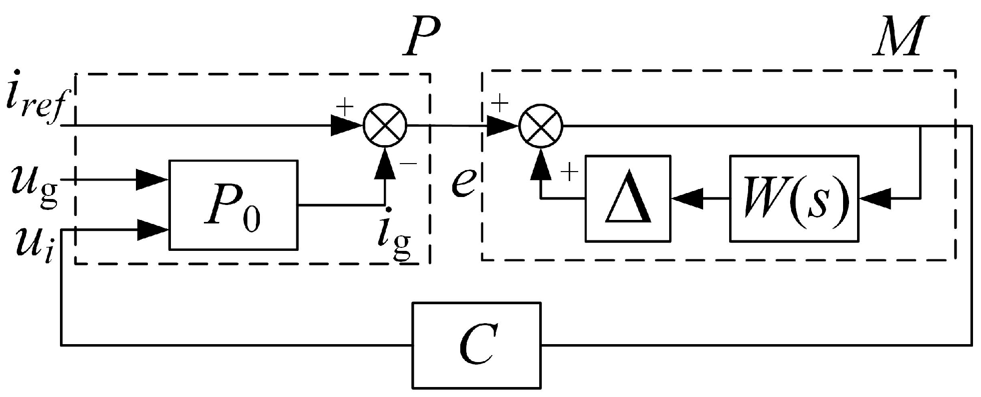
As mentioned in Section 2, the feedback line of ic is considered as part of the filter after equivalent transformation. Therefore, the model of the current control system shown in Figure 2 can be simplified (see Figure 4). P0 is the model of the LCL filter including the feedback line of ic and the feedback coefficient K, without considering the delay and ZOH units. Furthermore, the equivalent controlled plant P is defined based on the H∞ repetitive theory (Figure 4).
The internal model M consists of a positive feedback connection of a delay line Δ and a low-pass filter W. Furthermore, Δ is equal to e−τds. τd denotes the fundamental period of the periodic current reference iref. Theoretically, when W = 1, M is an infinite-dimensional internal model which introduces high gains at the fundamental and all harmonic frequencies [20]. To increase the stability margin, a low-pass filter W is introduced into the internal model. When M is adopted to control the output current, a compensator is always necessary to guarantee the stability of the system. The primary objective of the controller design method is to obtain the stabilizing compensator C by solving an H problem. To further simplify the design procedure, Kpwm was considered as part of C.
According to reference [22], the H∞ problem is formulated based on the state-space model of P. As shown in Figure 2 and Figure 4, P was defined based on the LCL filter model. Because the proportional feedback of the capacitor-current does not increase the order of P, is, ig, and uc were chosen as state variables, which can be expressed as x = [is ig uc]T. The phase voltage of PCC ug and the current reference iref were defined as the external input w, therefore, w = [ug iref]T. Considering control input u = ui and output y = e, the state-space model of P can be expressed as:
The model can also be presented as:
with:
As per Equation (3), the feedback coefficient K is part of the parameter matrix of the filter and can be considered as additional resistance. Therefore, the resonance of the filter can be damped by selecting the proper value of K. Furthermore, the unstable poles introduced by the LCL filter do not need to be compensated by C, which is helpful in simplifying the structure of the proposed controller.
3.2. Selection of Feedback Coefficient K Considering the Computation Delay
Although the proportional feedback of the capacitor-current can stabilize the equivalent controlled plant, further studies presented in references [9,10] indicated that the inappropriate value of K could introduce extra unstable poles due to computation delay and ZOH. While the stability compensator C was designed based on H∞ theory without considering the delay effects, the proposed RC cannot guarantee the stability of the system when it is implemented in practice. Therefore, the K value should be selected not only to provide sufficient damping, but also to avoid the introduction of unstable poles.
Based on Figure 2, by adopting the modified Z-transform, a discrete model of P0 can be obtained which includes the computation delay and ZOH unit. Additionally, the variation of the computation delay presented in Figure 3 was considered. The transfer function P0(z) can be expressed as:
where:
Define:
The transfer function of P0(z) can be derived as:
As shown in Figure 4, the transfer function of the equivalent controlled plant P = −P0 when w = 0. Thus, the stability of the controlled plant can be analyzed based on P0(z).
As per Equation (7), aside from z = 1, the other poles of P0(z) can be derived based on the equation:
According to reference [9], the increase of the feedback coefficient K can introduce a pair of unstable poles to the system. Because the unstable poles are caused by the delay of digital control, they cannot be stabilized by the compensator C, which is designed without considering the delay effects. As mentioned in Section 1, the valid region of the capacitor-current-feedback active damping can be extended by introducing an extra delay compensator [11,12,13] or reducing the computation delay [10].
As shown in Equation (3), the proportional feedback of capacitor current does not complicate the H∞ problem formulated to obtain C because this active damping method does not increase the order of P. However, the introduction of a delay compensator can complicate the model of the equivalent controlled plant. To avoid this, a variable computation delay is introduced as Figure 3 illustrated. By moving the sampling instant of the control signals close to the PWM reference update instant, the valid region of the active damping can be extended which also extends the safe region of K. This method can be implemented in a digital control processor through programming.
To simplify the design procedure, the direct relationship between the upper-limit of the feedback coefficient Kmax and computation delay Td was derived by applying Jury’s criterion to D(z). During the mathematical derivation, conditions fr < 1/4fs and K > 0 were required. The results can be summarized as follows:
- (1)
- If 0.5Ts ≤ Td ≤ Ts, a precise Kmax can be obtained by solving the inequality group. The upper-limit of K to avoid unstable poles of P0(z) can be expressed as:
- (2)
- If 0 ≤ Td < 0.5Ts, it is more complicated to obtain as precise a solution as in Case 1. However, a sufficient condition to avoid the unstable poles of P0 can be obtained, and the upper-limit of K is obtained as:While there are no existing unstable poles, the selection of K should also provide enough gain margin. Because a −180° crossing takes place at ω =ωr [10], the gain margin (GM) can be derived from Equation (7) as:
Considering the uncertainty of the compensator C, the damped LCL filter should have enough GM, which can provide more flexibility in the controller design based on H∞ theory. In this paper, GM > 10 dB is recommended in design practice. Therefore, another condition for the selection of K can be obtained as:
Based on Equations (9), (10), and (12), the region of K can be obtained to provide a reasonable stability margin, while not introducing unstable poles.
3.3. Compensator Calculation Based on H∞ Theory
Based on the proposed stable region, the value of K can be confirmed, and the state-space model of P can be obtained. Thus, the standard H∞ problem can be formulated to derive C. Based on references [22,24], the block diagram of the proposed H∞ problem is shown in Figure 5.
As Figure 5 illustrates, P is embedded into an augmented plant Pa, which has exogenous input wa = [v, w]T and external output za= [b, μui]T. Additionally, the control input u = ui, and the measurement output ya = e + λv. The parameters μ and λ are used to adjust the features of C [22]. Thus, by changing the values of μ and λ, compensator C can be found which helps the system achieve better stability.
The transfer function of W is shown as:
The state-space model of W can be expressed as:
Based on Equations (3), and (14), Pa can be obtained as:
According to Equation (15), a standard H∞ problem can be formulated. By solving the proposed H∞ problem using the MATLAB robust control toolbox, the compensator C can be obtained.
3.4. Stability Criterion for the Proposed H∞ Repetitive Control Scheme
Based on practical experience, the solution of the proposed H∞ problem is too complicated to be directly applied in a digital control system. Thus, the simplification and discretization of the proposed controller are necessary. To evaluate the stability of the control system with a simplified H∞ RC, a stable condition based on a continuous model of the system was presented in reference [22]. However, as preceding paragraphs have illustrated, the influence of computation delay and ZOH is not negligible in digital implementation. Therefore, a method to evaluate the stability of the system based on a discrete control model is proposed in this section.
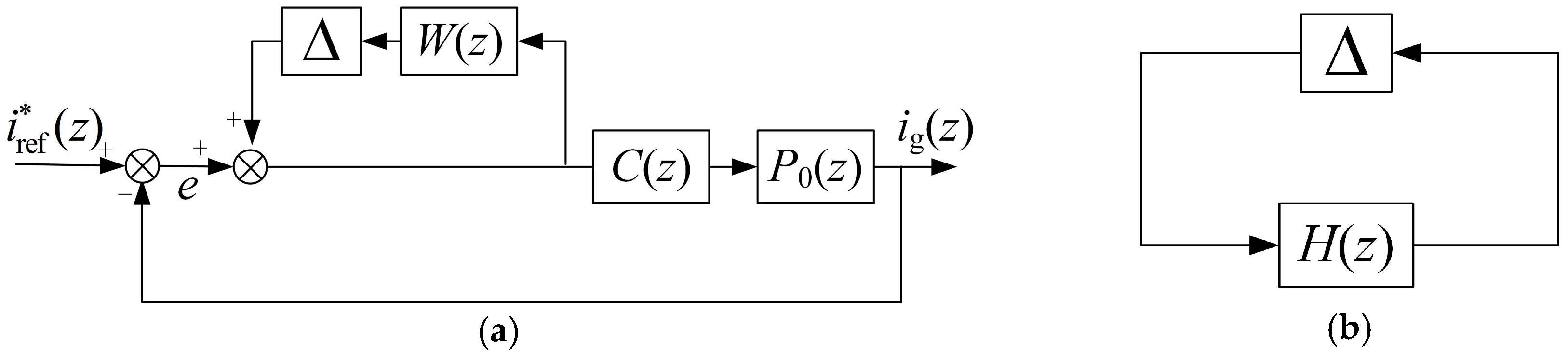
The diagram of the discrete current control system is shown in Figure 6a, where C(z) and W(z) can be obtained by applying Z transformation to C(s) and W(s). Δ is the delay line of the RC. If Δ is considered as an unknown perturbation, Figure 6a can be transferred to Figure 6b after a loop transformation and H(z) can be derived as:
Based on small gain theorem [25], when H(z) is stable, a sufficient condition for system stability can be derived as:
The stability criterion can be used in analyzing the selection of the control parameters and in studying the robustness of the control system.
4. Design Example and Stability Analysis
In this section, a design example of the proposed current controller is presented for a 10 kW three-phase grid-connected inverter. The inverter was built based on the circuit topology shown in Figure 1. Furthermore, the power circuit parameters of the inverter are given in Table 1.
As shown in Figure 1, a 130 V/400 V step-up transformer was used to increase the output voltage of the inverter, and the equivalent inductance of the transformer was included in Lg.
4.1. Selection of the Capacitor-Current-Feedback Coefficient
Prior to the design of the RC based on H∞ theory, it was necessary to select the value of the damping coefficient K. Based on the research carried out in Section 3.2, the region of K could be determined by the computation delay Td when the parameters of the LCL filter were certain. Based on the parameters presented in Table 1, fr was equal to 1.3 kHz, less than 1/4 fs. Thus, the region of K can be derived according to Equations (9), (10), and (12), and the result is shown in Figure 7.
As Figure 7 shows, the Kmax was improved by reducing the computation delay when 0.5 ≤ m ≤ 1. When 0 ≤ m < 0.5, the result based on Equation (10) provided a sufficient condition for avoiding the unstable poles of P0(z) and was considered as a reference to select the values of K and Td. The Kmin was obtained using Equation (12) as the GM restriction. It can be seen, in this example, that when Td = Ts, the value of K cannot fit both restrictions simultaneously. Therefore, to provide a larger gain margin, the value of K was selected as 3, while the Td was selected as 0.5Ts.
4.2. Controller Design Based on H∞ Theory
When K = 3, the state-space model of the plant P can be obtained as per Equations (2) and (3), and while wc is chosen as 2500, the transfer function of W can be expressed as:
By applying the Tustin transformation to Equation (18), the discrete transfer function of W can be obtained as:
The values of μ and λ can be adjusted to achieve better performance of the compensator C. In this case, μ = 10 and λ = 0.02. Based on Equation (15), the proposed H∞ problem was formulated. Thus, the transfer function of the compensator C can be obtained by solving the H∞ problem, which can be expressed as:
According to reference [24], the transfer function of C1(s) can be reduced to moderate the complexity of the compensator and the simplified compensator is:
The equivalent discrete transfer function of C2(s) can be derived by applying Tustin transformation to Equation (21), and can be expressed as:
As shown in Figure 4, the proposed RC is the series connection of internal model M and compensator C. The transfer function of M can be obtained based on the delay line Δ and W. Theoretically, the delay time of Δ, which is denoted as τd should be equal to the fundamental period of the reference current. However, due to the phase delay introduced by the low-pass filter W, Δ should be set slightly lower than the fundamental period [22,23], therefore, τd was set to 19.63 ms. To compare the performance between the continuous controller M(s)C1(s) and the simplified discrete controller M(z)C2(z), the bode plots of two controllers are shown in Figure 8.
As illustrated in Figure 8, the simplified discrete controller M(z)C2(z) keeps the amplitude frequency characteristics of M(s)C1(s) in a low frequency range. The discrete controller can provide high gains at the fundamental frequency and other harmonic frequencies like the 5th, 7th, 11th, and 13th harmonic frequencies. While the LCL filter attenuates the high frequency harmonics of the output current, the low frequency harmonics are the main reason for the increase of the THD level. Therefore, the proposed controller M(z)C2(z) can track the given current reference and compensate the main harmonic components of the output current. However, the simplified controller has different characteristics in a higher frequency region, which may cause a stability problem, especially when the computation delay and ZOH cannot be neglected. The stability of the discrete control system with the simplified H∞ repetitive current controller requires further evaluation.
4.3. Stability Analysis Considering the Impact of Computation Delay
Based on the parameters presented in Table 1, the discrete transfer function of P0(z) can be obtained as per Equation (7). Therefore, the transfer function of H(z) can be derived by substituting C2(z), W(z), and P0(z) into Equation (16).
According to the analysis presented in Section 4.1, when K = 3, the computation delay was selected as 0.5Ts to avoid the unstable poles caused by delay effects. To illustrate the relationship between system stability and computation delay, the stability analysis was carried out as Td was equal to 0.5Ts, 0.75Ts, and Ts, respectively.
According to the stability criterion, the necessary condition for the stability of the proposed system is that H(z) is stable. Figure 9a presents the poles of H(z) with variable Td. It is clear that a pair of poles move outside the unit cycle as Td increases, which destabilizes the current control system.
If H(z) is stable, the inequality Equation (17) should be satisfied to guarantee the stability of the system. While in a SISO system, the H∞ norm is equal to the maximum value of the frequency response magnitude. Thus, the locus of the vector |H(ejωTs)| should be inside the unit cycle if ||H(ejωTs)||∞ < 1. Figure 9b shows the locus of |H(ejωTs)| with a different Td.
The stability analysis can be summarized as follows:
Case A (Td = 0.5Ts): As shown in Figure 9a, no unstable poles of H(z) exist. According to Figure 9b, the locus of |H(ejωTs)| is inside the unit circle, and ||H(ejωTs)||∞ = 0.6025. Therefore, the stability condition is satisfied, and the proposed current control system is stable.
Case B (Td = 0.75Ts): As Figure 9a shows, a pair of poles of H(z) is close to the unit circle, but H(z) is stable at this time. However, according to Figure 9b, |H(ejωTs)| in this case is greater than unity, and ||H(ejωTs)||∞ = 1.9577, which does not satisfy the inequality Equation (17). As a result, the system is unstable.
Case C (Td = Ts): In this case, a pair of unstable poles of H(z) is shown in Figure 9a. As a result, even though the locus of |H(ejωTs)| is inside the unit circle, the system is still not stable.
In summary, the proposed current control system with the H∞ RC is stable and has a reasonable stability margin when Td = 0.5Ts.
4.4. Stability Analysis Considering the Variation of Grid-Impedance
When an LCL-type inverter is connected to the grid, the stability of the system is affected by the equivalent grid-impedance. In general, the grid-impedance is considered in series with the grid side inductor Lg. While the resistance of the grid-impedance can provide passive damping to the LCL filter, the inductance can decrease the resonance frequency of the LCL filter and makes the control system unstable [26]. Therefore, the proposed controller should be sufficiently robust against the variation of the inductance of grid-impedance.
The grid-impedance is considered as pure inductance for the worst case and is represented by the equivalent series inductor at the low-voltage side of the grid-connected transformer. Thus, when the power rating is 10 kW, the voltage rating is 130 V, and the equivalent inductance is considered up to 10% PU. As a result, the value of Lg varies from 0.3 to 0.8 mH.
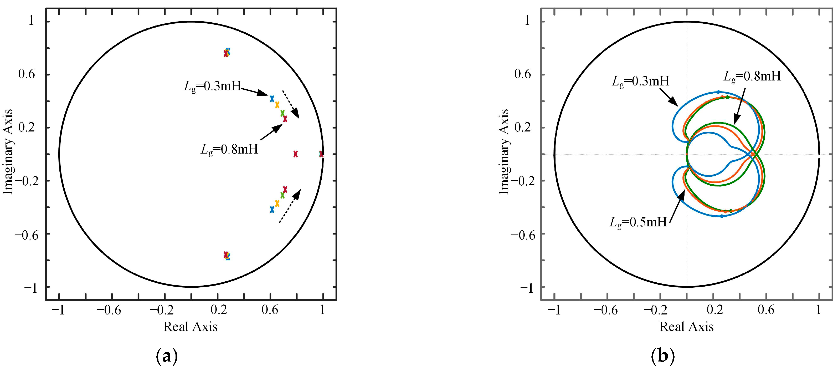
Figure 10a illustrates the poles of H(z) with the variation of Lg. When 0.3 mH ≤ Lg ≤ 0.8 mH, the poles of H(z) are inside the unit circle and H(z) is stable. The locus of |H(ejωTs)| with different Lg (Lg = 0.3 mH, 0.5 mH, and 0.8 mH, respectively) is shown in Figure 10b. While Lg increases, the |H(ejωTs)| remains inside the unit cycle and the ||H(ejωTs)||∞ varies from 0.603 to 0.625. In summary, the proposed system is stable with the variation of Lg and has reasonable stability margin.
5. Simulation and Experimental Results
According to the circuit topology (Figure 1) and the power circuit parameters (Table 1), a 10 kW three-phase grid-connected inverter was built in the laboratory to test the performance of the control scheme. A DSP (TMS320F28335) processor (Texas Instruments, Dallas, TX, USA) was selected to implement the current control scheme. Two high-accuracy analog-to-digital converters (MAX1320, Maxim Integrated, San Jose, CA, USA) were adopted to sample the voltage and current signals. The power switches used in the inverter were insulated-gate bipolar transistor modules FF450R12KT4 (Infineon, Munich, Germany). The maximum rated collector-emitter voltage and continuous collector current of the insulated-gate bipolar transistor (IGBT) were 1200 V and 450 A. As shown in Figure 1, the sinusoidal pulse width modulation (SPWM) was adopted in practice. The inverter was connected to the local distribution network through a 130 V/400 V transformer. The experimental setup is illustrated in Figure 11.
Furthermore, based on Equations (19) and (22), the discrete transfer function of the current controller GRC can be expressed as:
Additionally, the model of the grid-connected inverter along with the control scheme was built in MATLAB/Simulink (MathWorks, Natick, MA, USA) to verify the stability of the control system. As mentioned in Section 1, the dead-time of the power switches is one of the major causes of the output current harmonic distortion. Thus, the dead-time was considered in the simulation and experimental studies.
The introductions and conclusions for different test scenarios are summarized as follows:
- The stability verification of the proposed current control scheme is illustrated in Section 5.1. The results prove that the system with the proposed RC was stable when K = 3, Td = 0.5Ts, and the system could be destabilized when Td was increased to 0.75Ts or Ts.
- The steady-state responses of the current control scheme with proposed RC are illustrated in Section 5.2.1. A multi-frequency PR controller was designed and adopted in the same current control system as a comparative trial. The experiment results prove that the proposed RC could provide better harmonics rejection performance with lower control algorithm complexity.
- The steady-state responses with different grid-impedances are illustrated in Section 5.2.2. The results verify the robustness of the proposed RC against the variation of grid-impedance.
- The transient response of the proposed control scheme under the step change of the current reference is illustrated in Section 5.2.3.
5.1. Stability Verification Based on Simulation
An unstable current control system can lead to serious overcurrent and distortion of output power when the inverter is connected to the grid; therefore damage to the experimental device can be inevitable in this situation. Thus, the stability verification was carried out in a simulated environment, with the results shown in Figure 12.
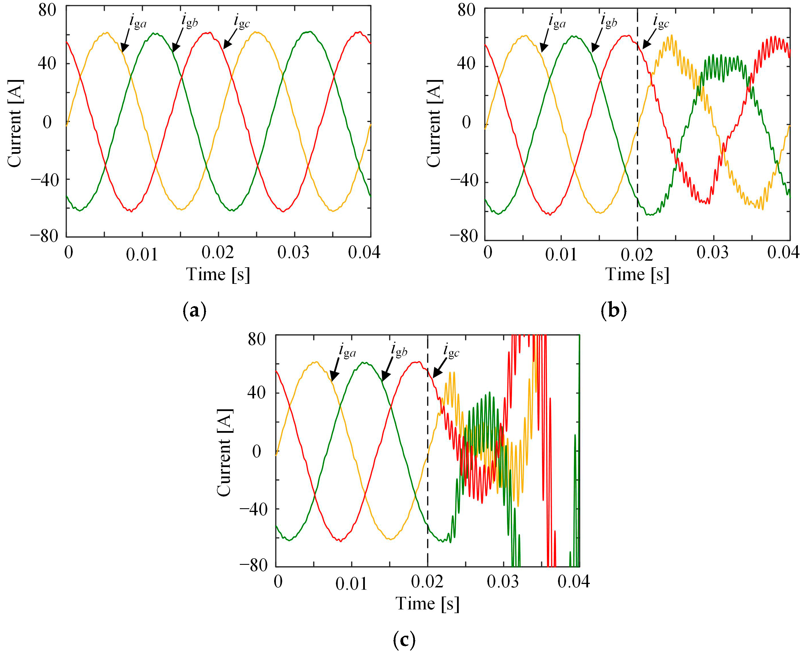
Figure 12a illustrates the full-load steady-state output current of the inverter when Td = 0.5Ts where a balanced three-phase current output with low harmonic content was achieved in this situation. In Figure 12b, Td was changed to 0.75Ts at 0.02 s, and it can be seen that a serious current distortion has occurred. In Figure 12c, Td was changed to Ts at 0.02 s, and the distorted output current increased rapidly after the change of computation delay.
Based on the simulation results, the analysis in Section 4.3 was verified and the current control system was unstable when Td = 0.75Ts or Td = Ts.
5.2. Experimental Results
5.2.1. Steady-State Responses
The proposed H∞ RC was implemented on the experimental platform and Td was set to 0.5Ts, based on the theoretical analysis and simulation results. Furthermore, a PR control scheme was designed based on references [5,10] with the same K and Td. As it is known that one single PR controller can provide high gain at a certain frequency, multiple PR controllers are always connected in parallel to track the given reference and compensate the harmonics. However, as each PR controller is 2-order, the implementation of the multi-PR control scheme causes much longer computation delay when compared with the proposed RC.
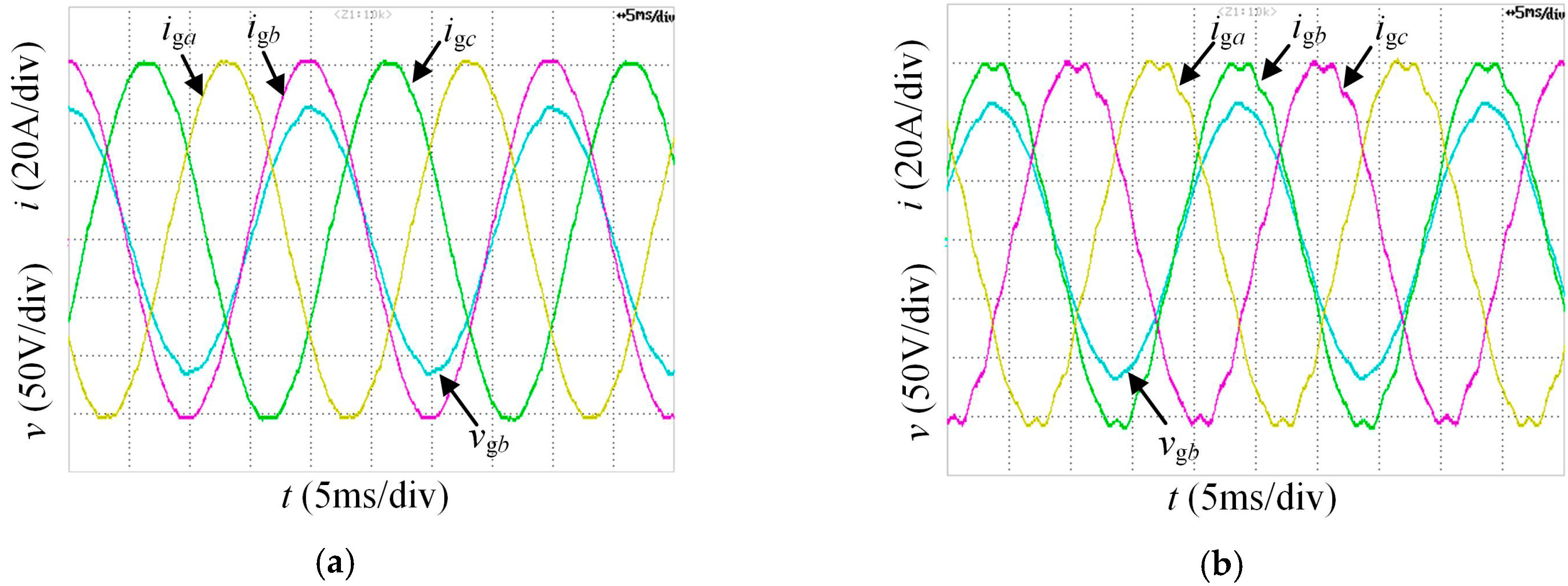
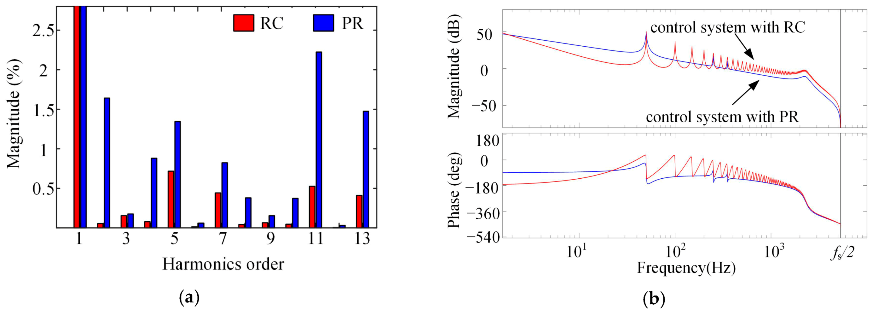
Considering the limited computation delay allowed in this scenario, three PR controllers were connected in parallel to track the fundamental current reference and reject the 5th and 7th harmonic currents. The PR scheme was implemented on the same platform as the comparative trial to verify the performance of the proposed RC current control scheme. Figure 13 shows the steady full-load output current of the grid-connected inverter with different controllers, and the waveforms of three-phase output current and the voltage of phase B at PCC are illustrated. The spectra of the output current of Phase A with different controllers are presented in Figure 14a.
As the spectra shows, the proposed RC can reject not only the 5th and 7th current harmonics as per the PR controller, but also the harmonics at other frequencies, such as the 2nd, 11th, and 13th. While the THD of the output current with the PR controller is 3.7483%, the THD decreased to 1.2321% when the proposed RC was adopted. The Bode plots of the current control systems with different controllers corroborated the harmonic analysis results. As shown in Figure 14b, the proposed RC could introduce higher open-loop gain at each harmonic frequency (including at the 5th and 7th harmonic frequencies). As a result, the output current had lower harmonic content. Although the introduction of W decreased the gains of the harmonic frequencies larger than the bandwidth of the low-pass filter, the H∞ RC was still very effective when the low-frequency output current harmonics are the major concern in practice.
5.2.2. Steady-State Responses with Different Grid-Impedance
To verify the robustness of the proposed RC against the variation of grid-impedance, an inductor was connected in series with Lg as the equivalent grid-impedance. As Section 4.4 describes, the experiment was carried out when Lg = 0.5 mH and 0.8 mH. As Figure 15 illustrates, the waveforms of output currents have rare differences when compared with Figure 13a, thus, the proposed control system was proven to be stable with the variation of the grid-impedance.
5.2.3. Transient Response
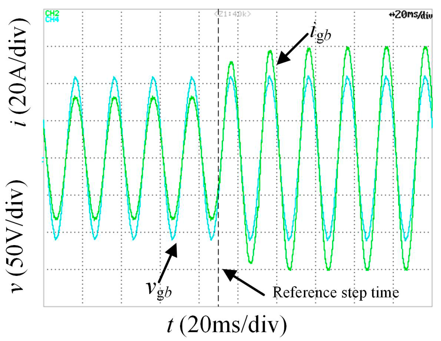
The transient response of the proposed controller was tested by stepping the output current reference from half-load to full load. The waveforms of the output current and voltage of Phase B at the time when the reference step occurred are shown in Figure 16.
6. Conclusions
A modified method is proposed in this paper to design an H∞ repetitive controller by considering the adoption of capacitor-current-feedback active damping and the delay of digital implementation. Compared with the traditional design method, the active damping is included in the H∞ repetitive controller design process by introducing an equivalent controlled plant which is built based on the model of the LCL-filter and the feedback of capacitor-current. Furthermore, the algebraic expression of the stable region for the feedback coefficient with variable computation delay is derived when the resonance frequency of LCL is less than 1/4fs. Thus, the unstable poles arising from digital control delay can be avoided by selecting reasonable values of the feedback coefficient and computation delay based on the stable region. Finally, the stability criterion for the discrete current control system with proposed non-linear RC is proposed in the paper.
As the simulation and experiment results illustrated, the H∞ repetitive control scheme (designed as per the proposed method) could guarantee system stability and showed high robustness under the variation of grid-impedance. Furthermore, when compared with the PR controller, the RC designed in this study showed excellent tracking and harmonic rejection performance with less computation complexity.
In this paper, the capacitor-current-feedback active damping was adopted to simplify the design procedure. However, different methods of active damping and delay compensation technologies have been proposed in recent studies. Thus, the applicability and the design technology for the H∞ repetitive control scheme based on other active damping methods needs to be researched in the next step. The design mentality and the stability criterion proposed in this paper can be helpful for future studies.
Acknowledgments
This work was supported by the National Natural Science Foundation of China under Award Number 51577128.
Author Contributions
Wei Jin developed the idea of the paper, and was responsible for the experimental design and paper writing; Yongli Li contributed to the discussion of the results and gave some suggestions; Guangyu Sun and Lizhi Bu helped to perform the experiments.
Conflicts of Interest
The authors declare no conflict of interest.
References
- Twining, E.; Holmes, D.G. Grid current regulation of a three-phase voltage source inverter with an LCL input filter. IEEE Trans. Power Electron. 2003, 18, 888–895. [Google Scholar] [CrossRef]
- Wu, W.M.; He, Y.B.; Tang, T.H.; Blaabjerg, F. A new design method for the passive damped LCL and LLCL filter-based single-phase grid-tied inverter. IEEE Trans. Ind. Electron. 2013, 60, 4339–4350. [Google Scholar] [CrossRef]
- Dannehl, J.; Fuchs, F.W.; Hansen, S.; Thogersen, P.B. Investigation of active damping approaches for PI-based current control of grid-connected pulse width modulation converters with LCL filters. IEEE Trans. Ind. Appl. 2010, 46, 1509–1517. [Google Scholar] [CrossRef]
- Xu, J.M.; Xie, S.J.; Tang, T. Active damping-based control for grid-connected LCL-filtered inverter with injected grid current feedback only. IEEE Trans. Ind. Electron. 2014, 61, 4746–4758. [Google Scholar] [CrossRef]
- Bao, C.L.; Ruan, X.B.; Wang, X.H.; Li, W.W.; Pan, D.H.; Weng, K.L. Step-by-Step controller design for LCL-type grid-connected inverter with capacitor-current-feedback active-damping. IEEE Trans. Power Electron. 2014, 29, 1239–1253. [Google Scholar]
- Xin, Z.; Wang, X.F.; Loh, P.C.; Blaabjerg, F. Digital realization of capacitor-voltage feedback active damping for LCL-filtered grid converters. In Proceedings of the 2015 IEEE Energy Conversion Congress and Exposition (ECCE), Montreal, QC, Canada, 20–24 September 2015; pp. 2690–2697. [Google Scholar]
- Tang, Y.; Loh, P.C.; Wang, P.; Choo, F.H.; Gao, F. Exploring inherent damping characteristic of LCL-filters for three-phase grid-connected voltage source inverters. IEEE Trans. Power Electron. 2012, 27, 1433–1443. [Google Scholar] [CrossRef]
- Wang, X.F.; Blaabjerg, F.; Loh, P.C. Grid-current-feedback active damping for LCL resonance in grid-connected voltage-source converters. IEEE Trans. Power Electron. 2016, 31, 213–223. [Google Scholar] [CrossRef]
- Parker, S.G.; McGrath, B.P.; Holmes, D.G. Regions of active damping control for LCL filters. IEEE Trans. Ind. Appl. 2014, 50, 424–432. [Google Scholar] [CrossRef]
- Pan, D.H.; Ruan, X.B.; Bao, C.L.; Li, W.W.; Wang, X.H. Capacitor-current-feedback active damping with reduced computation delay for improving robustness of LCL-type grid-connected inverter. IEEE Trans. Power Electron. 2014, 29, 3414–3427. [Google Scholar] [CrossRef]
- Wang, X.; Blaabjerg, F.; Loh, P.C. Virtual RC damping of LCL-filtered voltage source converters with extended selective harmonic compensation. IEEE Trans. Power Electron. 2015, 30, 4726–4737. [Google Scholar] [CrossRef]
- Li, X.Q.; Wu, X.J.; Geng, Y.W.; Yuan, X.B.; Xia, C.Y.; Zhang, X. Wide damping region for LCL-type grid-connected inverter with an improved capacitor-current-feedback method. IEEE Trans. Power Electron. 2015, 30, 5247–5259. [Google Scholar] [CrossRef]
- Xin, Z.; Wang, X.F.; Loh, P.C.; Blaabjerg, F. Grid-current-feedback control for LCL-filtered grid converters with enhanced stability. IEEE Trans. Power Electron. 2017, 32, 3216–3228. [Google Scholar] [CrossRef]
- Infield, D.G.; Onions, P.; Simmons, A.D.; Smith, G.A. Power quality from multiple grid-connected single-phase inverters. IEEE Trans. Power Deliv. 2004, 19, 1983–1989. [Google Scholar] [CrossRef]
- Espi, J.M.; Castello, J.; Garcia-Gil, R.; Garcera, G.; Figueres, E. An adaptive robust predictive current control for three-phase grid-connected inverters. IEEE Trans. Ind. Electron. 2011, 58, 3537–3546. [Google Scholar] [CrossRef]
- Sha, D.; Wu, D.; Liao, X. Analysis of a hybrid controlled three-phase grid-connected inverter with harmonics compensation in synchronous reference frame. IET Power Electron. 2011, 4, 743–751. [Google Scholar] [CrossRef]
- Alemi, P.; Bae, C.J.; Lee, D.C. Resonance suppression based on PR control for single-phase grid-connected inverters with LLCL filters. IEEE J. Emerg. Sel. Top. Power Electron. 2016, 4, 459–467. [Google Scholar] [CrossRef]
- Teodorescu, R.; Blaabjerg, F.; Liserre, M.; Loh, P.C. Proportional-resonant controllers and filters for grid-connected voltage-source converters. IEE Proc. Electr. Power Appl. 2006, 153, 750–762. [Google Scholar] [CrossRef]
- Shen, G.Q.; Zhu, X.C.; Zhang, J.; Xu, D.H. A new feedback method for PR current control of LCL-filter-based grid-connected inverter. IEEE Trans. Ind. Electron. 2010, 57, 2033–2041. [Google Scholar] [CrossRef]
- Zhang, K.; Kang, Y.; Xiong, J.; Chen, J. Direct repetitive control of SPWM inverter for UPS purpose. IEEE Trans. Power Electron. 2003, 18, 784–792. [Google Scholar] [CrossRef]
- Abusara, M.A.; Sharkh, S.M.; Zanchetta, P. Control of grid-connected inverters using adaptive repetitive and proportional resonant schemes. J. Power Electron. 2015, 15, 518–529. [Google Scholar] [CrossRef]
- Weiss, G.; Hafele, M. Repetitive control of MIMO systems using H∞ design. Automatica 1999, 35, 1185–1199. [Google Scholar] [CrossRef]
- Hornik, T.; Zhong, Q.C. H∞ repetitive voltage control of grid-connected inverters with a frequency adaptive mechanism. IET Power Electron. 2010, 3, 925–935. [Google Scholar] [CrossRef]
- Hornik, T.; Zhong, Q.C. A current-control strategy for voltage-source inverters in microgrids based on H∞ and repetitive control. IEEE Trans. Power Electron. 2011, 26, 943–952. [Google Scholar] [CrossRef]
- Francis, B.A. (Ed.) A Course in H∞ Control Theory; Springer-Verlag: Berlin, Germany, 1987; pp. 1–5. [Google Scholar]
- Liserre, M.; Teodorescu, R.; Blaabjerg, F. Stability of photovoltaic and wind turbine grid-connected inverters for a large set of grid impedance values. IEEE Trans. Power Electron. 2006, 21, 263–272. [Google Scholar] [CrossRef]
Figure 1.
Circuit topology of the grid-connected inverter and the diagram of the current control system in the αβ-domain.
Figure 1.
Circuit topology of the grid-connected inverter and the diagram of the current control system in the αβ-domain.

Figure 2.
Block diagram of the single-phase current control system.
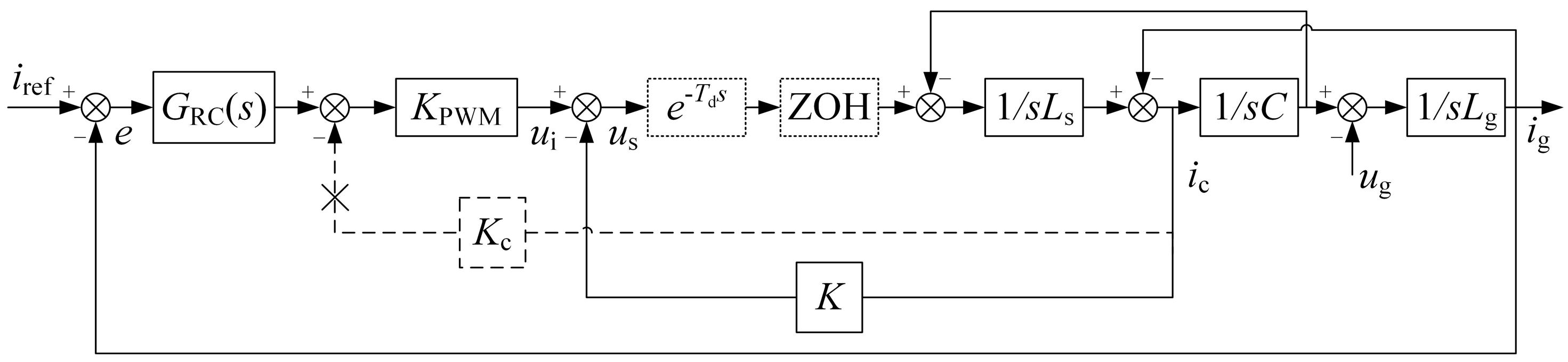
Figure 3.
Delay mechanism in the digital control.
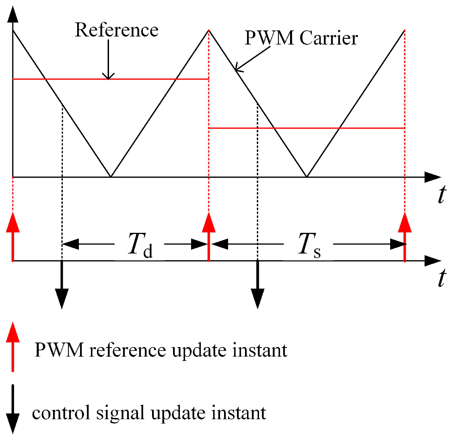
Figure 4.
Block diagram of the current control scheme with the proposed controller.

Figure 5.
Block diagram of the standard H∞ problem.
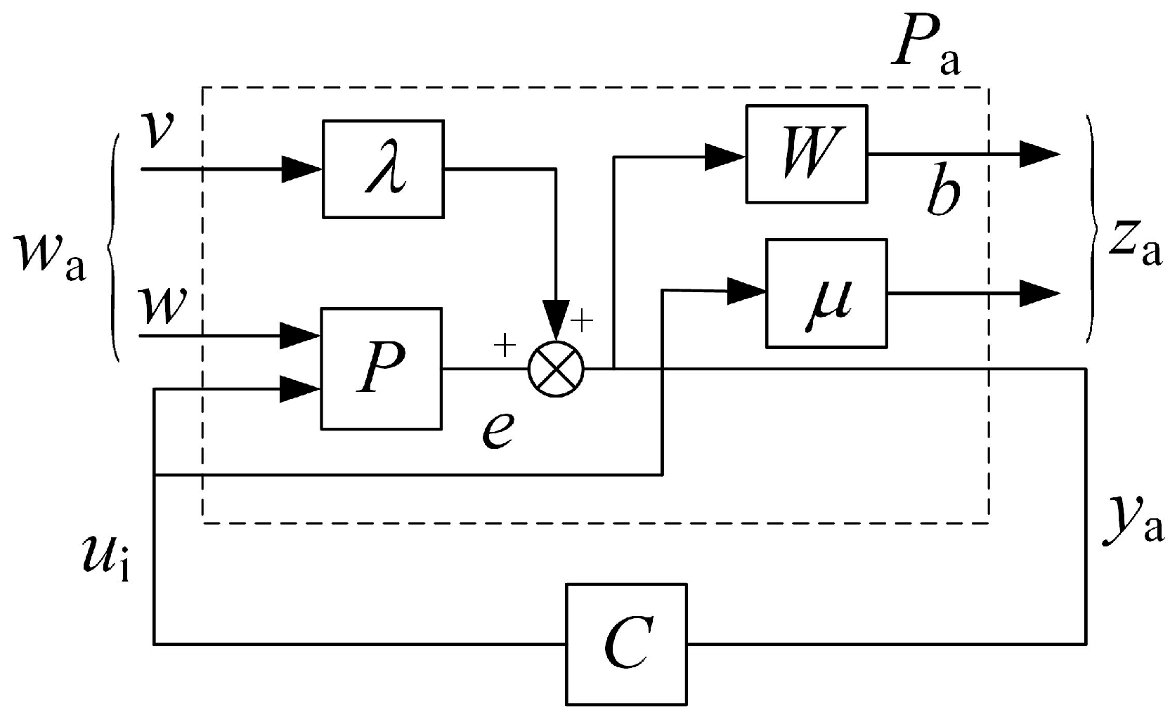
Figure 6.
Block diagram of the discrete current control system. (a) Complete model; and (b) after loop transformation.
Figure 6.
Block diagram of the discrete current control system. (a) Complete model; and (b) after loop transformation.

Figure 7.
Region of K with variable Td (Td = mTs, 0 ≤ m ≤ 1).
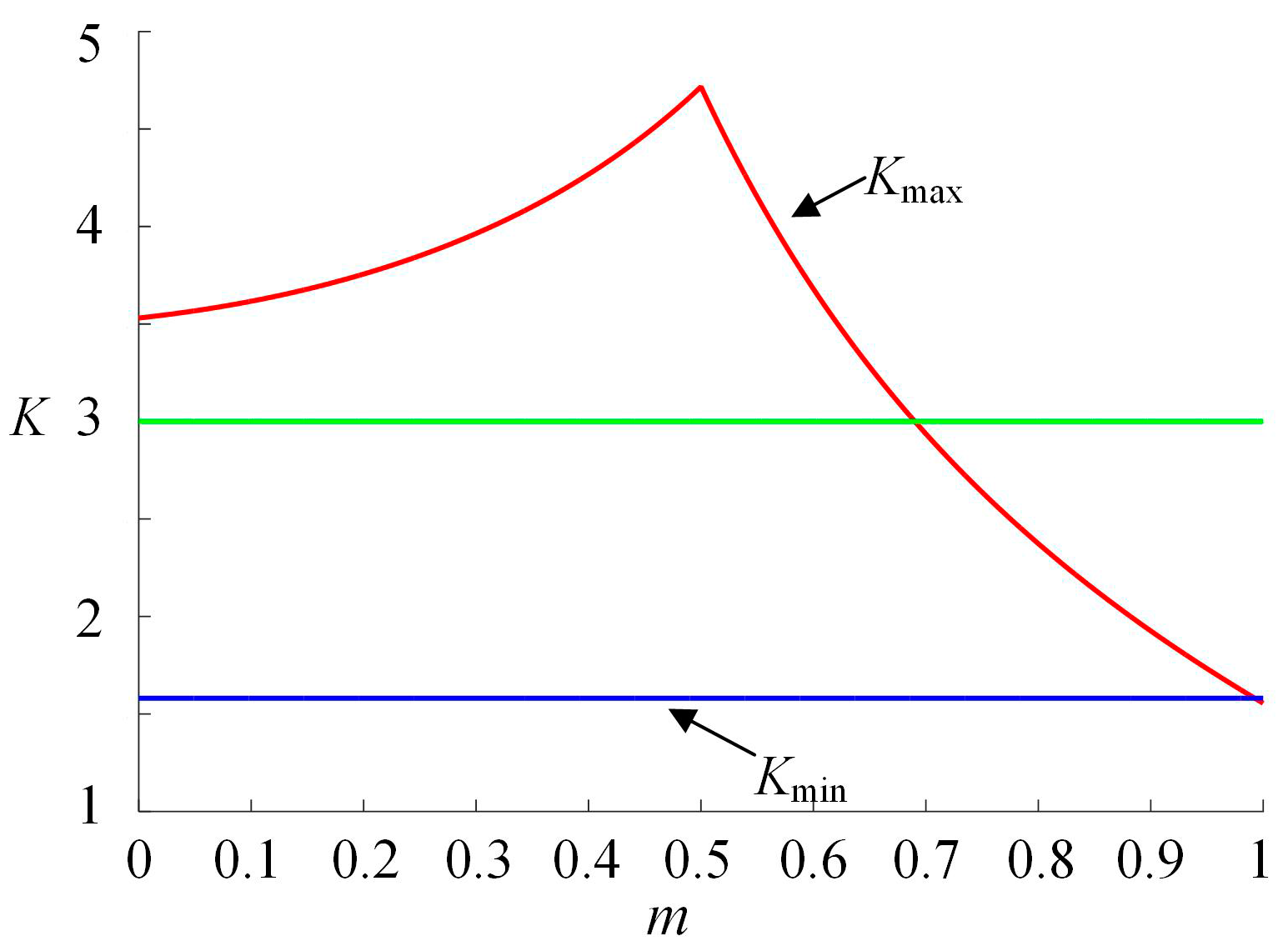
Figure 8.
Bode plots of M(s)C1(s) and M(z)C2(z).
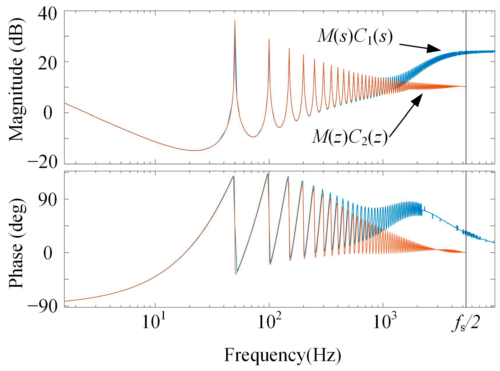
Figure 9.
Stability analysis for the system with variable Td (Td = mTs, 0 ≤ m ≤ 1). (a) Pole map of H(z); and (b) locus of the vector |H(ejωTs)|.
Figure 9.
Stability analysis for the system with variable Td (Td = mTs, 0 ≤ m ≤ 1). (a) Pole map of H(z); and (b) locus of the vector |H(ejωTs)|.
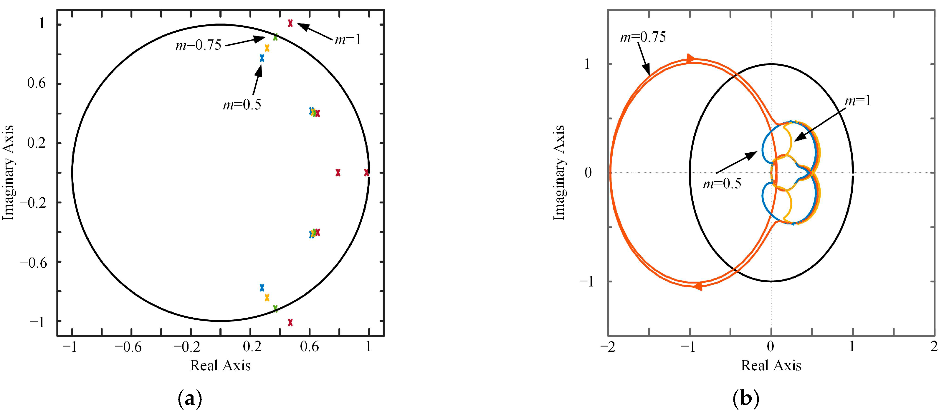
Figure 10.
Stability analysis for the system with variable Lg. (a) Pole map of H(z); and (b) locus of the vector |H(ejωTs)|.
Figure 10.
Stability analysis for the system with variable Lg. (a) Pole map of H(z); and (b) locus of the vector |H(ejωTs)|.

Figure 11.
The experimental setup for the current control scheme test.
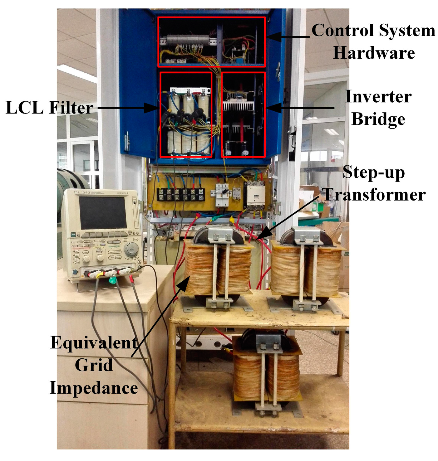
Figure 12.
Steady-state full-load output current with different computation delays. (a) Td = 0.5Ts; (b) Td = 0.75Ts; and (c) Td = Ts.
Figure 12.
Steady-state full-load output current with different computation delays. (a) Td = 0.5Ts; (b) Td = 0.75Ts; and (c) Td = Ts.

Figure 13.
Steady-state full-load output current with different control strategies. (a) RC; and (b) PR.
Figure 13.
Steady-state full-load output current with different control strategies. (a) RC; and (b) PR.

Figure 14.
(a) Spectra of output current; and (b) Bode plots of the control system open-loop gain with different controllers.
Figure 14.
(a) Spectra of output current; and (b) Bode plots of the control system open-loop gain with different controllers.

Figure 15.
Steady-state full-load output current with different equivalent grid-impedances. (a) Lg = 0.5 mH; and (b) Lg = 0.8 mH.
Figure 15.
Steady-state full-load output current with different equivalent grid-impedances. (a) Lg = 0.5 mH; and (b) Lg = 0.8 mH.
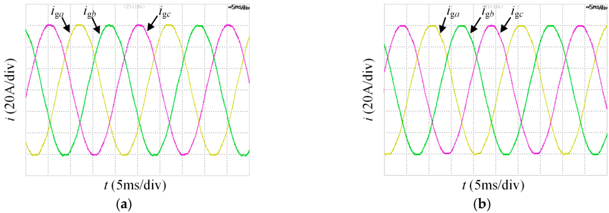
Figure 16.
Transient response of the proposed grid-connected inverter.


Table 1.
Power circuit parameters of the grid-connected inverter.
| Parameters | Values |
|---|---|
| Inverter-side inductance, Ls | 0.3 mH |
| Grid-side inductance, Lg | 0.3 mH |
| Filter capacitor, C | 100 μF |
| Nominal grid frequency, fg | 50 Hz |
| Nominal grid voltage, Un | 380 V (rms) |
| Sampling frequency, fs | 10,650 Hz |
| Switching frequency, fsw | 10,650 Hz |
| Power rating, Pn | 10 kW |
| DC Voltage, Udc | 450 V |
Table 2.
Parameters of the Current Control Scheme.
| Parameters | Values |
|---|---|
| Pulse-width-modulation (PWM) gain, Kpwm | 225 |
| Equivalent feedback coefficient, K | 3 |
| Feedback coefficient, Kc | 0.0133 |
| Delay time of the repetitive controller, τd | 19.63 ms |
| Cutoff frequency of the low-pass filter, wc | 2500 rad/s |
| Amplitude of active current reference, Id_ref | 65 A |
| Amplitude of reactive current reference, Iq_ref | 0 A |
© 2017 by the authors. Licensee MDPI, Basel, Switzerland. This article is an open access article distributed under the terms and conditions of the Creative Commons Attribution (CC BY) license (http://creativecommons.org/licenses/by/4.0/).
Share and Cite
MDPI and ACS Style
Jin, W.; Li, Y.; Sun, G.; Bu, L. H∞ Repetitive Control Based on Active Damping with Reduced Computation Delay for LCL-Type Grid-Connected Inverters. Energies 2017, 10, 586. https://doi.org/10.3390/en10050586
AMA Style
Jin W, Li Y, Sun G, Bu L. H∞ Repetitive Control Based on Active Damping with Reduced Computation Delay for LCL-Type Grid-Connected Inverters. Energies. 2017; 10(5):586. https://doi.org/10.3390/en10050586
Chicago/Turabian StyleJin, Wei, Yongli Li, Guangyu Sun, and Lizhi Bu. 2017. "H∞ Repetitive Control Based on Active Damping with Reduced Computation Delay for LCL-Type Grid-Connected Inverters" Energies 10, no. 5: 586. https://doi.org/10.3390/en10050586
Note that from the first issue of 2016, this journal uses article numbers instead of page numbers. See further details here.