
Comparison of Solar Radiation Models to Estimate Direct Normal Irradiance for Korea

1
School of Mechanical Engineering, Kookmin University, 77 Jeongneung-ro, Seongbuk-gu, Seoul 02727, Korea
2
New and Renewable Energy Resource Center, Korea Institute of Energy Research, 152 Gajeong-ro, Yuseong-gu, Daejeon 34129, Korea
*
Authors to whom correspondence should be addressed.
Energies 2017, 10(5), 594; https://doi.org/10.3390/en10050594
Submission received: 10 February 2017
/
Revised: 17 April 2017
/
Accepted: 20 April 2017
/
Published: 30 April 2017
(This article belongs to the Section L: Energy Sources)
Abstract
:Reliable solar radiation data are important for energy simulations in buildings and solar energy systems. Although direct normal irradiance (DNI) is required for simulations, in addition to global horizontal irradiance (GHI), a lack of DNI measurement data is quite often due to high cost and maintenance. Solar radiation models are widely used in order to overcome the limitation, but only a few studies have been devoted to solar radiation data and modeling in Korea. This study investigates the most suitable solar radiation model that converts GHI into DNI for Korea, using measurement data of the city of Daejeon from 2007 to 2009. After ten existing models were evaluated, the Reindl-2 model was selected as the best. A new model was developed for further improvement, and it substantially decreased estimation errors compared to the ten investigated models. The new model was also evaluated for nine major cities other than Daejeon from the standpoint of typical meteorological year (TMY) data, and consistent evaluation results confirmed that the new model is reliably applicable across Korea.
1. Introduction
Continuous global energy issues, such as climate change and energy shortages, have increased the interest in energy-efficient buildings and solar energy systems. The energy simulation of such systems is critical for accurate performance evaluation and, ultimately, for optimal design. As the most important input to the energy simulation, reliable solar radiation data must be given in advance. The most useful solar radiation data are global horizontal irradiance (GHI), but direct normal irradiance (DNI) or diffuse horizontal irradiance (DHI) are also important. For example, irradiance on the surface of a solar collector or solar cell is determined when either DNI or DHI is given in addition to the GHI [1]. Note that the GHI, DNI, and DHI are interdependent and, thus, knowing two irradiances out of three is sufficient.
Solar radiation measurements are often limited to a few locations or short-term periods in some countries. Furthermore, in general, availability of DNI (or DHI) data is much lower than that of GHI data because DNI measurement using a sun tracker costs more and needs more careful maintenance. Along with research efforts for energy-efficient buildings and solar energy systems, the demand for DNI data has increased significantly in Korea [2,3]. Even though the Korea Meteorological Administration (KMA) provides GHI data, as well as other meteorological data, such as dry bulb temperature and wind speed, DNI is not included [4]. When DNI data are not available, it is necessary to rely on a solar radiation model that accounts for regional climate characteristics. Many solar radiation models to estimate DNI with GHI have been developed [5,6]. However, only a few studies have been devoted to solar radiation data and modeling for Korea, and even fewer studies to hourly DNI data. A lack of DNI measurement data has been a major obstacle to meaningful studies. Recently, Lee et al. [7] modeled GHI with cloud cover data for major cities in Korea and, successively, Lee et al. [8] reported a solar radiation model developed for estimating DNI with GHI. However, the model of Lee et al. [8] tends to underestimate DNI data such that DNI values exceeding 750 W/m2 seldom occur.
Long-term, 20 or 30 years, solar radiation data collected on an hourly basis are desirable to reflect climatic characteristics at a specific location and obtain reliable simulation results [9]. Since a direct handling of massive data is burdensome, representative datasets generated from raw, long-term data are often used. The representative data, usually referred to as the typical meteorological year (TMY) data, contain 8760 hourly values of meteorological elements for the one-year duration [10,11]. The Korean Solar Energy Society (KSES) has shared the TMY data of seven cities in Korea but, unfortunately, its TMY datasets reveal unreasonably low DNI values [12]. As a result, the users relying on the TMY data from KSES have a risk of underestimating DNI effects in their energy simulations.
This study aims at investigating solar radiation models, including a newly developed model, for the estimation of DNI from GHI in Korea and providing a guideline for the selection of solar radiation models in energy simulations. In the beginning, ten well-known solar radiation models are evaluated with three years of data from the city of Daejeon in Korea. Then, a new model based upon the quasi-physical approach proposed by Maxwell [13] is presented. Finally, from the standpoint of the TMY data, variations of solar irradiance due to the solar radiation model are analyzed, and the nationwide extension of the new model is investigated.
2. Evaluation of Existing Solar Radiation Models
KMA as a national representative provides meteorological data over 100 locations [4]. GHI is also available at some locations, but DNI is not available at all. Meanwhile, Korea Institute of Energy Research (KIER) measured both GHI and DNI in the city of Daejeon for research purpose. In this study, KIER measurement data from 2007 to 2009 were used for evaluation of solar radiation models and for development of a new model. The city of Daejeon is located approximately at the center of Republic of Korea, and its latitude, longitude, and altitude are 36.18°, 127.24°, and 77.1 m, respectively. The pyranometer for GHI measurement was a CMP 11 model from Kipp & Zonen Company in Delft, the Netherlands whereas the pyrheliometer for DNI measurement was a CHP 1 model with a SOLYS 2 sun tracker from the same company. Both GHI and DNI were measured every minute and averaged over 60 min to get hourly data. The uncertainties originated from both of the sensors are less than 1%. Based on references [14,15] and experiences, the estimated measurement uncertainties of GHI and DNI are generally 3% on the average and 5% at most. For the three years, the average percentages of missing GHI and DNI data were 2.3% and 1.9%, respectively. The data pair that misses either GHI or DNI and was measured when the zenith angle of the sun was larger than 85° were excluded. The number of the remained pairs of GHI and DNI measurements totals 11,928.
Solar radiation models to estimate DNI can be classified into two categories, parametric and decomposition models [5]. In parametric models, solar radiation is obtained from other meteorological parameters, such as cloud cover, atmospheric turbidity, pressure, and water content. On the other hand, decomposition models rely on correlations between global, direct, and diffuse components of solar radiation. Whereas parametric models require detailed information of the atmospheric conditions, decomposition models are relatively easy to use once the GHI is known. Out of many decomposition models, ten were selected in this study: Orgill and Hollands [16], Vignola and McDaniels [17], Louche et al. [18], Lee et al. [8], Lam and Li [19], CIBSE [20], Erbs et al. [21], Maxwell [13], and two from Reindl et al. [22]. These models are widely used for modeling solar radiation, e.g., in relevant textbooks [1] and in model comparison studies [5,8,23]. The selected models were evaluated by comparing the modeled and the measured DNI data.
Most of the decomposition models use correlations between global, direct, and diffuse solar radiation. Once the global, direct, diffuse, and extraterrestrial irradiances on a horizontal surface are given by , , , and , respectively, three non-dimensional parameters—the clearness index, , the direct beam transmittance, , and the diffuse fraction, —can be defined. Note that represents GHI. DNI is denoted by and is related to by the equation of , in which is the zenith angle of the sun.
Usually, the correlations of a solar radiation model render or as a function of in separate intervals divided by values. If a model yields rather than , DNI is calculated via after is obtained. Only three models among the ten models evaluated in this study are presented in the following for brevity. The Lee model [8] is selected because it was recently developed with measurement data from the city of Daejeon in 2009. The Reindl-2 [22] and Maxwell [13] models are selected because they show good performances compared to the others, which will be demonstrated later. The Reindl-2 model was developed with measurement data at five European and North American locations, and the term of is added as the second input parameter besides . The Maxwell model will be explained in the next section. The rest of the other models can be found in the corresponding articles.
Except for the Maxwell model, the correlations for or are a polynomial function of . The only difference lies in the coefficients that account for climate characteristics where the solar irradiance data were measured and used for developing each model. Meanwhile, the Maxwell model possesses a different functional form because the quasi-physical approach is applied; that is, it, in part, reflects the physics involved in the atmospheric transmission of solar radiation.
In order to identify proper models for Korea, DNI values were calculated with the ten candidate models using the selected GHI data as the input and compared with actual DNI measurement data. Linear regression analysis between measured and modeled DNI data was conducted for each model. Based on the regression analyses, the ten models were divided into three groups from the standpoint that the estimation is larger than the measurement and high DNI values of more than 750 W/m2 are properly estimated. The first group, which includes the Orgill, the Vignola, the Louche, the Erbs, the Reindl-1, and the Lam models, estimates DNI values larger than the measurement and yields unacceptably high values from time to time. Figure 1a shows the scatterplot obtained with the Vignola model as a representative of the first group. Some estimated DNI values exceeded 1000 W/m2, but such high DNI values are very rarely observed in Korea.
On the contrary, the Lee and the CIBSE models, which belong to the second group, seldom yield high DNI values, resulting in underestimation. Figure 1b shows the scatter plot obtained with the Lee model as a representative of the second group. The linear regression trend beyond DNI values exceeding 750 W/m2 slopes downward, suggesting that additional correlation at large should be introduced. Even though the Lee model was developed with the DNI measurement data in Korea [8], its underestimation implies that one-year data used for the model development are not enough for proper estimation.
The third group includes the Reindl-2 and the Maxwell models. These models estimate DNI values larger than those measured, but they do not pose extreme behaviors, in contrast to those in the first and the second groups. Lave et al. [23] demonstrated that the Reindl-2 and the Maxwell models use the term of (via air mass in the Maxwell model) in addition to and, thus, they outperform other models that use only, which is consistent with this study. The observation frequency, normalized by dividing with the total number of data points, was calculated according to the level of the DNI. Histograms of the normalized data shown in Figure 2 indicate that the Reindl-2 model suitably estimates the observation frequency of DNI values in each DNI bin. On the other hand, the Maxwell model tends to overestimate DNI values in the bins from 750 to 950 W/m2. However, when the scatterplots in Figure 1c,d are compared, it is clear that with the Reindl-2 model the DNI is occasionally estimated too high.
The coefficient of determination (R2), the mean bias error (MBE), the root mean square error (RMSE), and the median absolute deviation (MAD) were calculated to distinguish the goodness-of-fit of each model and summarized in Table 1. The models do not alter R2 values remarkably, roughly in the variation range of 2%, and the R2 of the Reindl-2 model is the best. The MBE is defined as the sum of the measurements minus the estimation. Therefore, a negative value of MBE means overestimation of a model, and a positive value means the opposite. Whereas the MBE is a good measure for yearly-based estimation, the RMSE is for hourly-based estimation. If the best model was to be selected from the ten investigated models, the first selection criterion is to exclude extreme behaviors. Accordingly, out of the third group, with better statistics of MBE and RMSE the Reindl-2 model becomes the most suitable for estimating the DNI in Korea. The unacceptable underestimation of the DNI disqualifies the CIBSE and the Lee models even though their MBEs are smaller. Note that the RMSE values in Table 1 roughly range from 25% to 35% of the mean DNI value and are significantly larger than the measurement uncertainty by approximately 3%.
3. Development of a New Solar Radiation Model
3.1. Methodology
In the previous section, the Reindl-2 model turned out to be the most suitable model. However, it is not entirely satisfactory. Above all, the MBE is still large, and some outliers can occur, as indicated in Figure 1c. An effort to improve the solar radiation model was made. The Reindl-2 and the Maxwell models naturally became good candidates due to the aforementioned comparison results. The Reindl-2 model uses a simple curve-fitting approach. Hence, the modification based on the quasi-physical approach of the Maxwell model [13] is likely to be a better estimate for Korea.
Maxwell’s quasi-physical approach was established upon the three following assumptions: First, air mass, , is the dominant parameter affecting the relationship between and . Second, using a physical model to calculate clear-sky will provide a physically-based reference, from which changes in can be calculated. Third, the seasonal, annual, and climate variations in the relationship between and are entirely accounted for by parametric functions in that relate to , cloud cover, and precipitable water vapor. The second hypothesis explains Equation (6) above. If clear-sky is defined as for limiting values, represents the deviation from it. Maxwell [13] adopted the Bird clear-sky model for , which corresponds to Equation (7). According to the first and third hypotheses that were obtained from statistical analyses, has a functional form, as in Equation (8). The coefficients A, B, and C in Equation (8) were determined by fitting solar radiation data from Atlanta, Georgia, USA in 1981.
Development of a new solar radiation model based on the quasi-physical approach starts from accepting Equations (6)–(8). Then, the remaining task is to determine the coefficients A, B, and C using solar radiation data from Korea, which will give rise to correlations similar to Equations (9)–(14). The first step is to divide into the intervals whose median values increase by 0.05, starting at 0.25, and in each interval of the regression analysis between and is carried out. For example, Figure 3 shows the scatterplot from the regression analysis at , in which the results represent very cloudy conditions, as indicated by the range of . Therefore, they correspond to the limiting case of , implying that the extraterrestrial solar radiation is completely absorbed or scattered by the atmosphere and, thus, the direct normal component of solar radiation is essentially zero. The black thin curve in Figure 3 represents in Equation (7), and the fact that all of the data in Figure 3 are located below this curve supports this statement.
The similar regression analyses (not presented) to determine the coefficients A, B, and C were repeated at each interval of until . Note that Maxwell [13] presented the regression analyses up to because was not available in the solar radiation data from Atlanta. For Daejeon, Korea, there are some solar radiation data even when , but they are not enough to derive statistically meaningful fits. The reason is that the solar radiation in the southeastern region of the US is more abundant than in Northeastern Asia. After the coefficients A, B, and C were determined at each interval of , another regression analysis was carried out in order to fit A, B, and C as a function of . The development procedure can be summarized as follows:
- Calculate , , and on an hourly basis ( is calculated based on [13]).
- Calculate and with the measured GHI, and DNI, .
- Divide the intervals of and the group data by the interval.
- Conduct a regression analysis between and and determine the coefficients A, B, and C in each group.
- Conduct another regression analysis to fit the coefficients A, B, and C as a function of .
Figure 4 shows that the coefficients A and B can be expressed as a linear function and a third-order polynomial function over the entire range, respectively. Meanwhile, the fitting of the coefficient C with a third-order polynomial function is required for separating into the two ranges, and . Similarly to the derivation of the original model by Maxwell [13], extrapolation is also applied in this study when . Finally, the correlations in the solar radiation model developed with the data from Daejeon, Korea can be written as follows:
3.2. Results
The scatterplot with the new model in Figure 5 is qualitatively similar to the counterpart in Figure 1d. It significantly reduces the occasional outliers estimated by the Reindl-2 model shown in Figure 1c. The goodness-of-fit is greatly improved with the new model. Table 1 shows the MBE and the RMSE are significantly improved with respect to the Reindl-2 model, by a factor of 8.7 and by 9.8%, respectively. However, the normalized frequency in Figure 2 demonstrates that the new model is slightly poorer than the Reindl-2 model in estimating high DNI exceeding 750 W/m2.
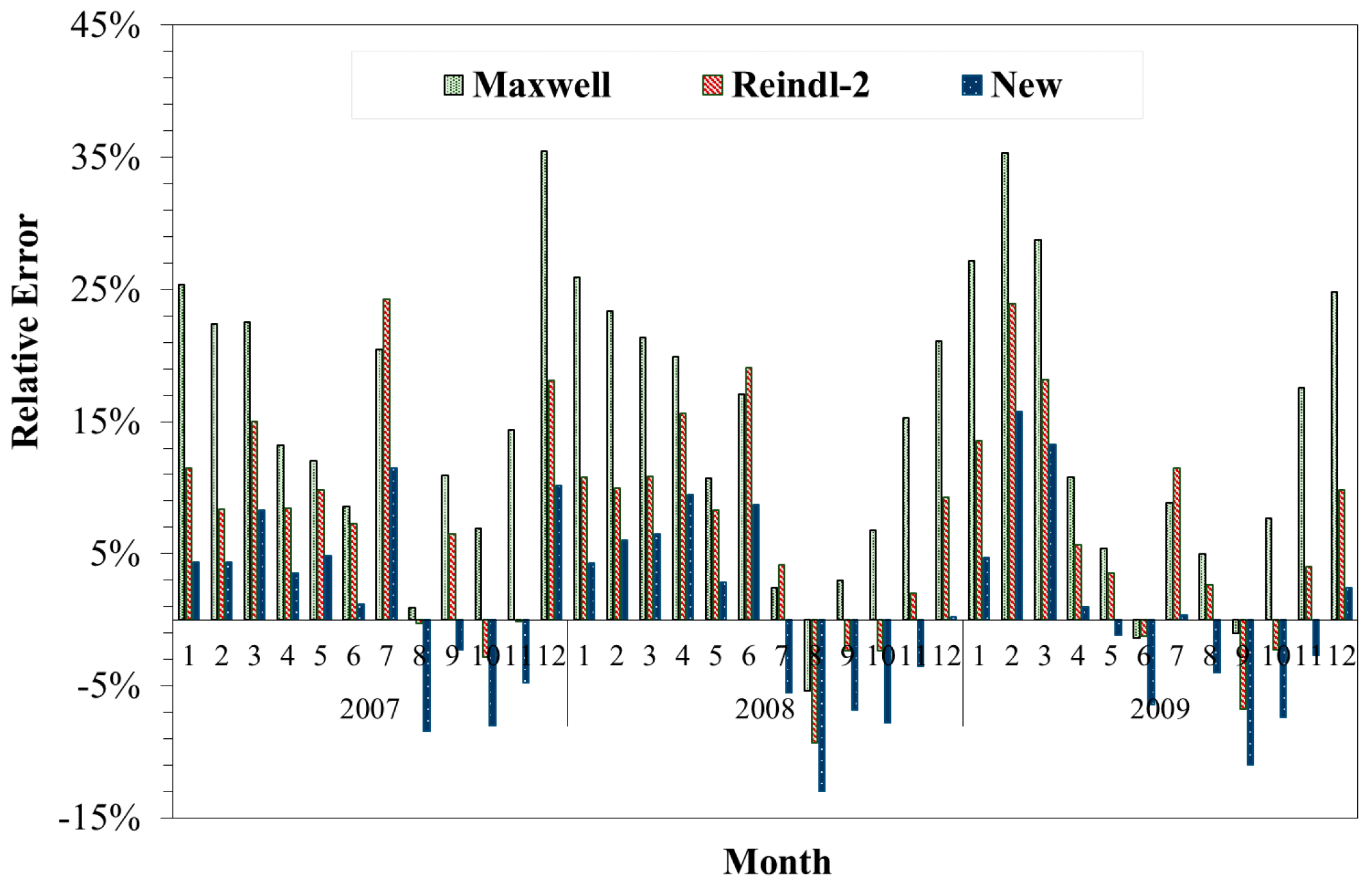
As summarized in Table 2, the error of the yearly sum of DNI supports that the new model remarkably improves estimation performance. For all three years—2007, 2008, and 2009—the error in estimation does not exceed 1.5%. Figure 6 shows variations of errors for estimating the monthly sum. In general, the new model leads to smaller errors compared to the Maxwell and the Reindl-2 models. The largest error for the Maxwell model is 35.5% in February 2009 and 24.3% for the Reindl-2 model in July 2007. However, the largest error for the new model is only 15.7% in February 2009. Errors are remarkably decreased around the winter and the spring seasons, whereas they are increased in several months of the summer and the autumn seasons. The new model tends to estimate DNI values smaller than the Maxwell and the Reindl-2 models regardless of the month, thereby resulting in the overall downward shifts of monthly errors in Figure 6. In order to investigate the effects of seasonal positions of the sun, the hourly errors in June 2009 and December 2009 against the solar zenith angle, , are presented in Figure 7. The smaller estimation by the new model is essentially independent of , which is generally true for the non-presented months as well. Consequently, it can be concluded that the underestimation of the new model consistently occurs throughout a year and contributes to decreasing the largest monthly error. Since the months where errors are decreased dominate those where errors are increased, performance in the yearly estimation is improved. In spite of better estimation in yearly irradiances, caution must be paid when the new model is applied for estimating monthly irradiances around the summer and the autumn seasons.
4. Variations of Solar Irradiance in TMY Data
Since the DNI measurement data of other cities in Korea were not accumulated systematically and sufficiently, the previous results obtained with data from the city of Daejeon cannot be directly validated for the nationwide extension. The ten major cities in Korea, including Daejeon, are considered: Busan, Cheongju, Daegu, Gangneung, Gwangju, Incheon, Jeju, Jeonju, and Seoul. The solar radiation models were compared in terms of the TMY data instead of the data of a specifically-selected year. Since the TMY data represent regional climatic characteristics for the one-year duration, they are generally used for energy simulations and facilitate evaluation [10]. In the following, TMY data of each city were generated after DNI was estimated with solar radiation models. Then, variations of solar irradiance were investigated to identify similar trends across the ten major cities.
A TMY dataset consists of the months selected from individual years and concatenated to form a complete year. In this study, the method of National Renewable Energy Lab (NREL) in the US was adopted for generation of TMY data [10]. The first step is to select five candidate months close to the long-term weather characteristics for each month. For the selection, monthly cumulative distribution functions (CDFs) for the daily data of a weather element are compared with the long-term CDF. According to the Finkelstein-Schafer (FS) statistics in Equation (19) [24], the deviation of the CDF of a specific month from the long-term CDF is calculated for the j-th weather element, in which the subscript n indicates the number of days in a month and denotes daily data on i-th day:
The ten weather elements in Table 3 are judged to be more important than the others, and a weighted sum of the FS statistics is used to select the five candidate months.
In the second step, the five candidate months are ranked with respect to the closeness of the month to the long-term mean and median. The third step is to check the persistence of the mean dry bulb temperature and daily GHI so that the month that exhibits exceptional weather patterns, such as the longest run or zero runs of consecutive warm days, are excluded. The highest-ranked candidate month from the second step that survives in the third step is selected as the typical meteorological month. Finally, in the fourth step, the 12 typical meteorological months are concatenated to form a complete year.
TMY data of the ten major cities in Korea were generated with 20-year (1991–2010) weather data from KMA [4]. Figure 8 shows that the yearly sums of the GHI in the TMY datasets do not change noticeably by solar radiation models, indicating their variations of not more than 2.1%. The yearly sums from all of the four models agree well with the 20-year long-term mean values within 3.0%. Accordingly, the effect of solar radiation models on the GHI is insignificant, although solar radiation models are used to obtain the DNI, which is involved in calculation of the FS statistics with the largest weight, as in Table 3. Note that the typical meteorological months are selected according to their ranking in the weighted sum of the FS statistics given by Equation (20). The DNI effects are likely to be addressed via the GHI because both the GHI and DNI have strongly positive correlation. Meanwhile, an important implication to investigate solar radiation models is to provide guideline to correct the current TMY data from KSES, which seriously underestimate the DNI [12]. The GHI data from KSES are generally smaller than the long-term means. However, if the city of Incheon showing 7.0% difference is excluded, the GHI data from KSES are still within the variation range by the solar radiation model.
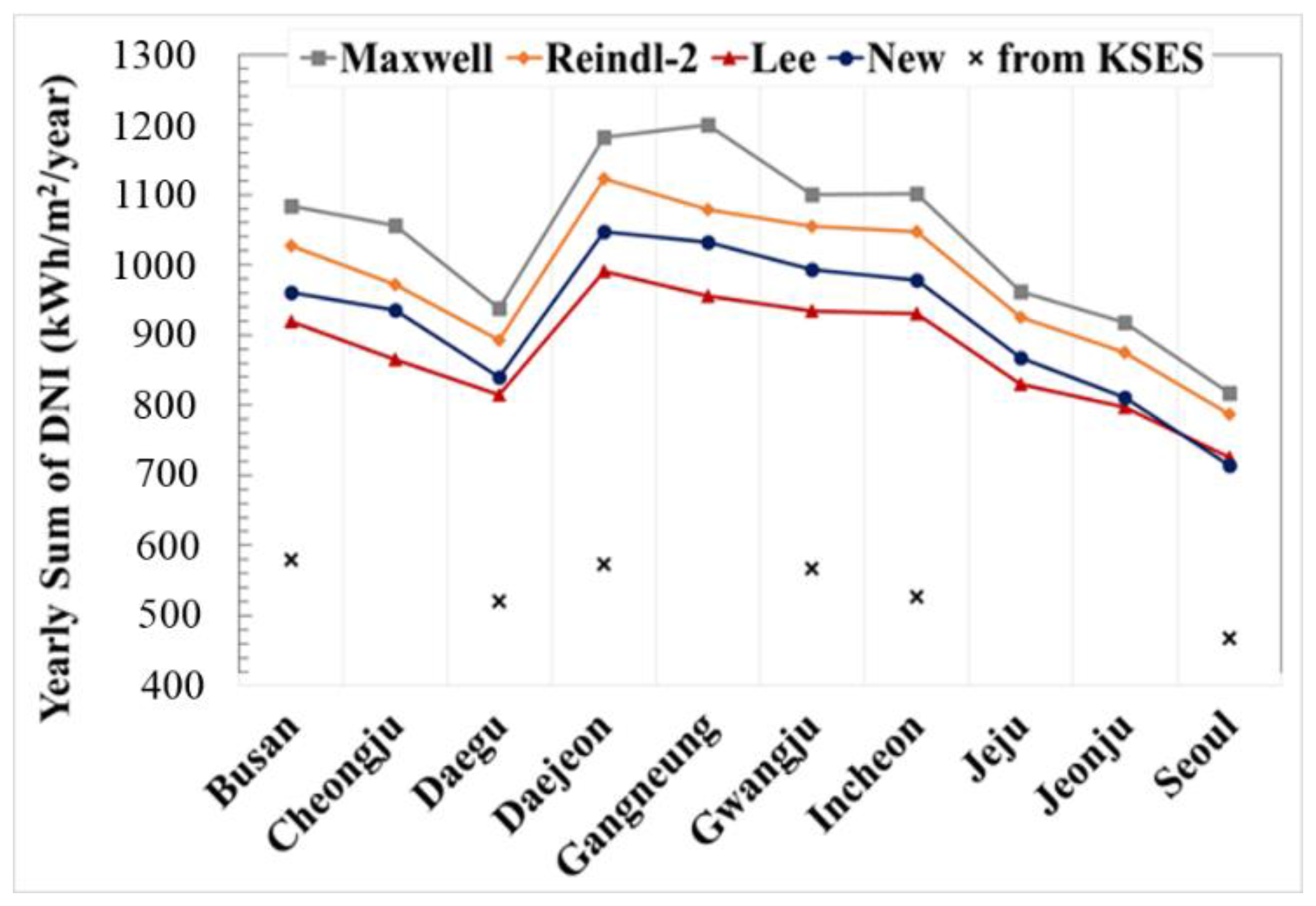
Figure 9 shows the yearly sums of the DNI in the TMY datasets. Compared to the GHI in Figure 8, the DNI variations by solar radiation model are increased. The Maxwell model estimates larger values by 18% on the average of the ten cities than the Lee model, while the Reindl-2 and the new models estimate larger values by 11.5% and 4.6%, respectively. The reverse order of the MBE values in Table 1 out of the Maxwell, the Reindl-2, the new, and the Lee models is consistent with the order of lines in Figure 9 (MBE is defined as measurement minus estimation). When the monthly sums of the DNI were analyzed for the nine other cities of Korea, similar seasonal variations due to solar radiation models were observed, as demonstrated in Figure 6. The consistent observations made with the nine other cities imply that the results based on the city of Daejeon should be applicable over the whole country. Meanwhile, the TMY data from KSES largely underestimate the yearly sums of the DNI such that they range from 53.8% to 65.5% of the counterparts from the new model. If the TMY data from KSES are used in energy simulation, the simulation results will not account for DNI effects properly.
5. Conclusions
Using solar radiation data from the city of Daejeon from 2007 to 2009, ten decomposition models that convert the GHI into the DNI were evaluated. It was demonstrated that the Orgill, Vignola, Louche, Erbs, Reindl-1, and Lam models estimated some DNI values to be unacceptably larger than 1000 W/m2. On the contrary, the Lee and CIBSE models tend to underestimate high DNI values exceeding 750 W/m2. The Reindl-2 and Maxwell models did not pose the extreme behaviors. According to the MBE and the RMSE, the Reindl-2 model was selected as the most suitable model for Korea.
A new model based on the quasi-physical approach was developed in order to improve error statistics and remove occasional outliers. The new model resulted in significantly reduced values of MBE and RMSE compared to the Reindl-2 model, by a factor of 8.7% and by 9.8%, respectively. The largest error in the monthly sum of the DNI is also reduced from 24.3% of the Reindl-2 model to 15.7% while the yearly sums of the DNI are estimated within an error of 1.5%. When comparisons were extended to ten major cities in Korea from the standpoint of the TMY data, consistent observations in the bias trend and the seasonal variation between the models were made and, thereby, support that the evaluation results in this study are applicable throughout the nation.
This study provides a guideline not only for selecting a suitable solar radiation model in Korea, but also for evaluating solar radiation models in Northeastern Asia. Weather data in energy simulation programs, such as PVsyst, TRNSYS (TRaNsient SYstem Simulation Program), and SAM, can be updated accordingly for reliable results. Furthermore, relations between irradiance components and with weather elements become more important as irradiance forecast technology advances [25]. This study will help satellite-based forecasting of solar resources in the long-term or in a broad region.
Acknowledgments
This work was financially supported by grants from the Korea Institute of Energy Technology Evaluation and Planning (KETEP), the Ministry of Trade, Industry, and Energy (MOTIE) (No. 20143010071570), and the National Research Foundation of Korea (NRF), Ministry of Education (2015M3D2A1032828).
Author Contributions
Hyun-Jin Lee and Chang-Yeol Yun conducted and conceived the project; Chang-Yeol Yun measured and analyzed the data; Shin-Young Kim classified the data and collected the materials; and Hyun-Jin Lee evaluated the models.
Conflicts of Interest
The authors declare no conflict of interest.
Abbreviation
| CDF | Cumulative Distribution Function |
| CIBSE | Chartered Institution of Building Services Engineers |
| GHI | Global Horizontal Irradiance |
| DHI | Diffuse Horizontal Irradiance |
| DNI | Direct Normal Irradiance |
| FS | Finkelstein-Schafer |
| KIER | Korea Institute of Energy Research |
| KMA | Korea Meteorological Administration |
| KSES | Korean Solar Energy Society |
| MBE | Mean Bias Error |
| RMSE | Root Mean Square Error |
| TMY | Typical Meteorological Year |
References
- Duffie, J.A.; Beckman, W.A. Solar Engineering of Thermal Processes, 3rd ed.; John Wiley & Sons: Somerset, NJ, USA, 2013. [Google Scholar]
- Lee, H.J.; Kim, J.K.; Lee, S.N.; Kang, Y.H. Numerical study on optical performances of the first central-receiver solar thermal power plant in Korea. J. Mech. Sci. Technol. 2016, 30, 1911–1921. [Google Scholar] [CrossRef]
- Vu, N.H.; Shin, S. A concentrator photovoltaic system based on a combination of prism-compound parabolic concentrators. Energies 2016, 9, 645. [Google Scholar] [CrossRef]
- Korea Meteorological Administration (KMA). Available online: https://data.kma.go.kr/cmmn/main.do (accessed on 8 February 2017).
- Wong, L.; Chow, W. Solar radiation model. Appl. Energy 2001, 69, 191–224. [Google Scholar] [CrossRef]
- Mousavi Maleki, S.A.; Hizam, H.; Gomes, C. Estimation of hourly, daily and monthly global solar radiation on inclined surfaces: Models re-visited. Energies 2017, 10, 134. [Google Scholar] [CrossRef]
- Lee, K.; Yoo, H.; Levermore, G.J. Generation of typical weather data using the ISO test reference year (TRY) method for major cities of South Korea. Energy Build. 2010, 45, 956–963. [Google Scholar] [CrossRef]
- Lee, K.; Yoo, H.; Levermore, G.J. Quality control and estimation hourly solar irradiation on inclined surfaces in South Korea. Renew. Energy 2013, 57, 190–199. [Google Scholar] [CrossRef]
- Sengupta, M.; Habte, A.; Kurtz, S.; Dobos, A.; Wilbert, S.; Lorenz, E.; Stoffel, T.; Renné, D.; Gueymard, C.A.; Myers, D. Best Practices Handbook for the Collection and Use of Solar Resource Data for Solar Energy Applications; National Renewable Energy Laboratory: Golden, CO, USA, 2015. [Google Scholar]
- Wilcox, S.; Marion, W. Users Manual for TMY3 Data Sets; National Renewable Energy Laboratory: Golden, CO, USA, 2008. [Google Scholar]
- Zang, H.; Wang, M.; Huang, J.; Wei, Z.; Sun, G. A hybrid method for generation of typical meteorological years for different climates of China. Energies 2016, 9, 1094. [Google Scholar] [CrossRef]
- Korean Solar Energy Society (KSES). Available online: http://www.kses.re.kr/data_06/list_hi.php (accessed on 8 February 2017).
- Maxwell, E.L. A Quasi-Physical Model for Converting Hourly Global Horizontal to Direct Normal Insolation; Solar Energy Research Institute: Golden, CO, USA, 1987. [Google Scholar]
- Myers, D.R. Solar radiation modeling and measurements for renewable energy applications: Data and model quality. Energy 2005, 30, 1517–1531. [Google Scholar] [CrossRef]
- Habte, A.; Sengupta, M.; Andreas, A.; Wilcox, S.; Stoffel, T. Intercomparison of 51 radiometers for determining global horizontal irradiance and direct normal irradiance measurements. Sol. Energy 2016, 133, 372–393. [Google Scholar] [CrossRef]
- Orgill, J.; Hollands, K. Correlation equation for hourly diffuse radiation on a horizontal surface. Sol. Energy 1977, 19, 357–359. [Google Scholar] [CrossRef]
- Vignola, F.; McDaniels, D. Beam-global correlations in the Pacific Northwest. Sol. Energy 1986, 36, 409–418. [Google Scholar] [CrossRef]
- Louche, A.; Notton, G.; Poggi, P.; Simonnot, G. Correlations for direct normal and global horizontal irradiation on a French Mediterranean site. Sol. Energy 1991, 46, 261–266. [Google Scholar] [CrossRef]
- Lam, J.C.; Li, D.H. Correlation between global solar radiation and its direct and diffuse components. Build. Environ. 1996, 31, 527–535. [Google Scholar] [CrossRef]
- Guide, J. Weather, Solar and Illuminance Data; Chartered Institution of Building Services Engineers (CIBSE): London, UK, 2002. [Google Scholar]
- Erbs, D.; Klein, S.; Duffie, J. Estimation of the diffuse radiation fraction for hourly, daily and monthly-average global radiation. Sol. Energy 1982, 28, 293–302. [Google Scholar] [CrossRef]
- Reindl, D.T.; Beckman, W.A.; Duffie, J.A. Diffuse fraction correlations. Sol. Energy 1990, 45, 1–7. [Google Scholar] [CrossRef]
- Lave, M.; Hayes, W.; Pohl, A.; Hansen, C.W. Evaluation of global horizontal irradiance to plane-of-array irradiance models at locations across the United States. IEEE J. Photovolt. 2015, 5, 597–606. [Google Scholar] [CrossRef]
- Finkelstein, J.M.; Schafer, R.E. Improved goodness-of-fit tests. Biometrika 1971, 58, 641–645. [Google Scholar] [CrossRef]
- Kleissl, J. Solar Energy Forecasting and Resource Assessment; Academic Press: Cambridge, MA, USA, 2013. [Google Scholar]
Figure 1.
Scatterplots of direct normal irradiance (DNI) measurements and estimations, in which the red curves represent the linear regression fits: (a) Vignola; (b) Lee; (c) Reindl-2; and (d) Maxwell.
Figure 1.
Scatterplots of direct normal irradiance (DNI) measurements and estimations, in which the red curves represent the linear regression fits: (a) Vignola; (b) Lee; (c) Reindl-2; and (d) Maxwell.
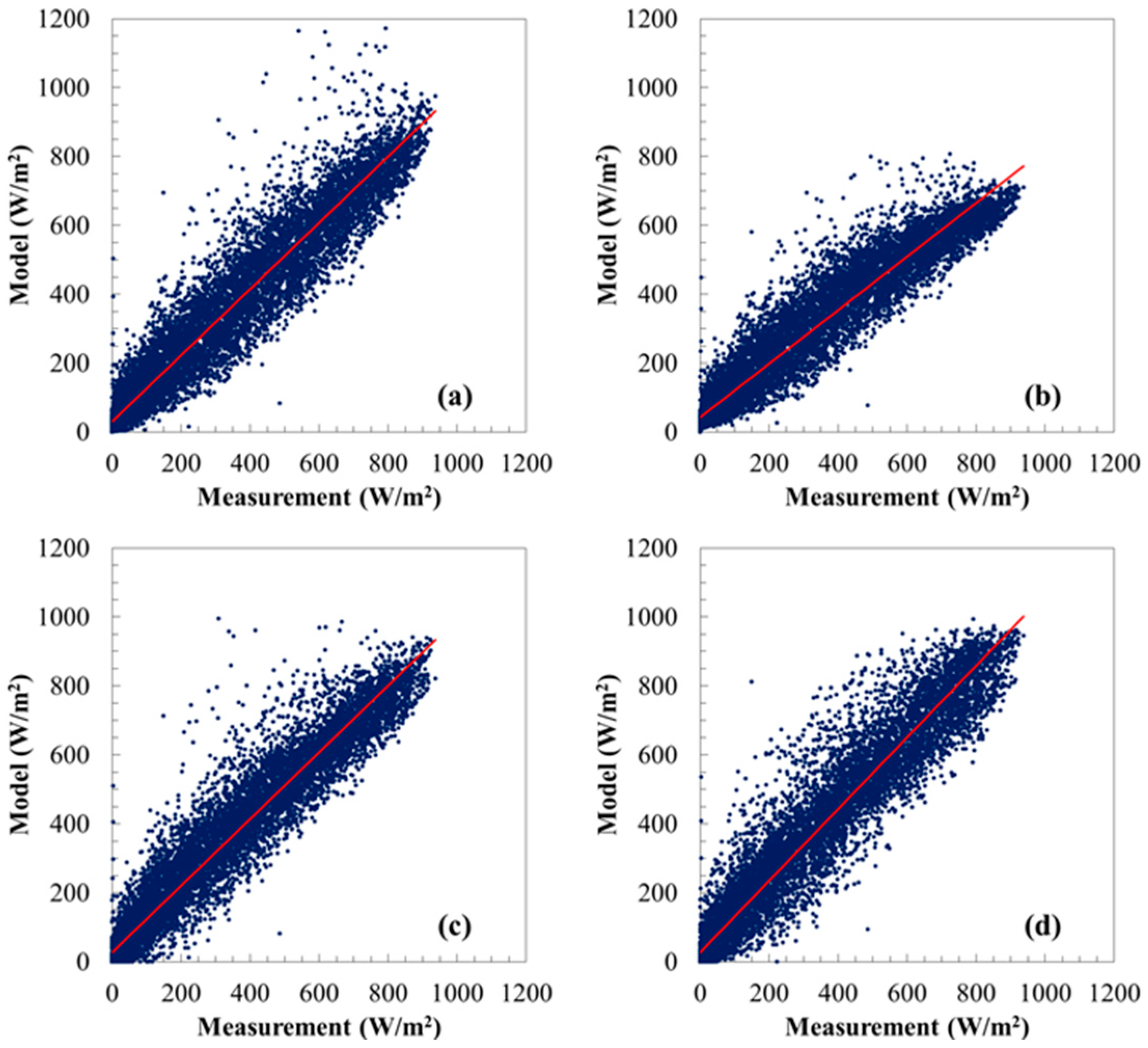
Figure 2.
Histograms of DNI measurement and estimation, in which frequency is normalized by dividing by the total number of data points.
Figure 2.
Histograms of DNI measurement and estimation, in which frequency is normalized by dividing by the total number of data points.
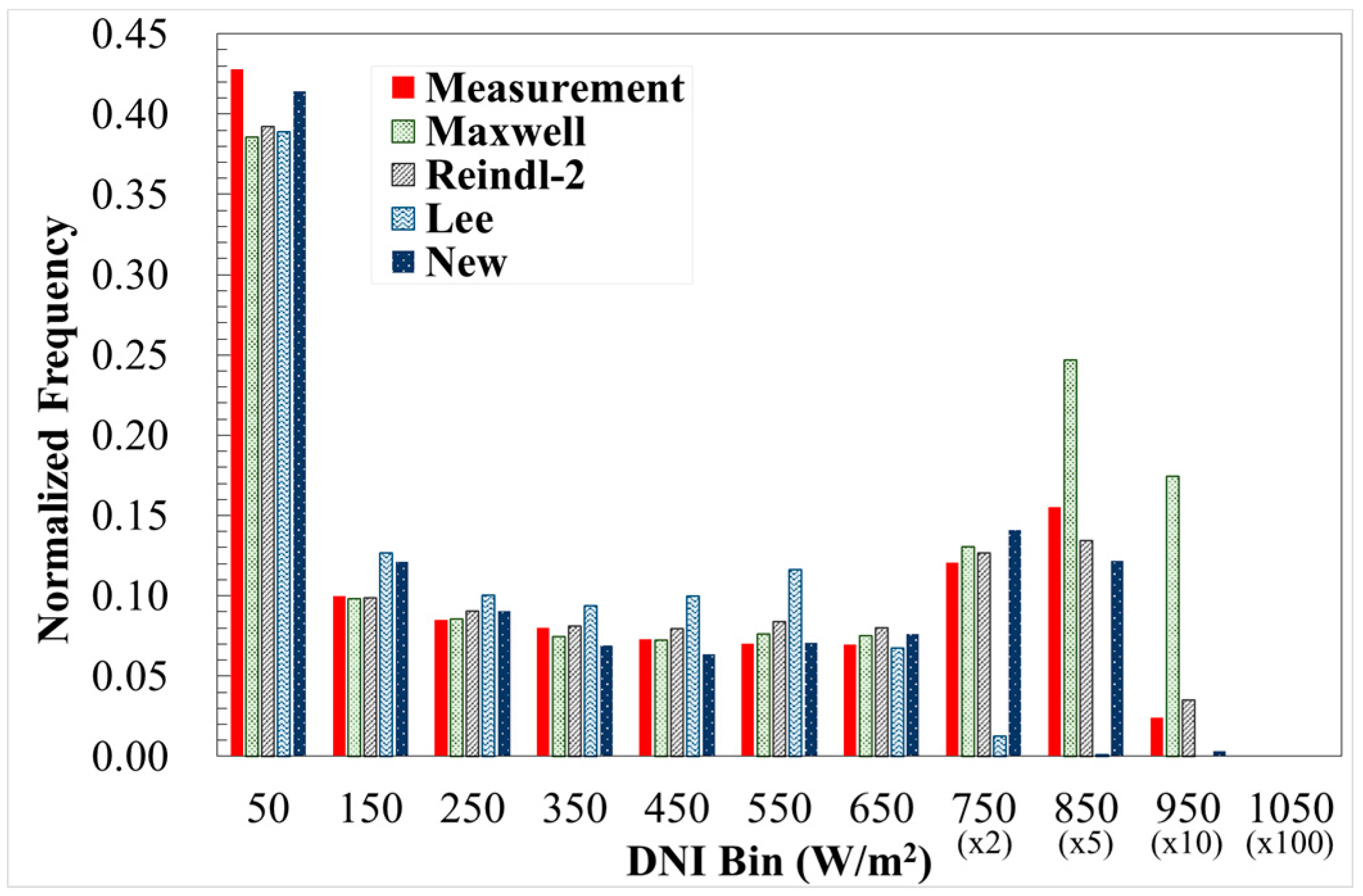
Figure 3.
Scatterplot of and the air mass at , in which the solid red curve represents the regression fit and the black thin curve represents in Equation (7).
Figure 3.
Scatterplot of and the air mass at , in which the solid red curve represents the regression fit and the black thin curve represents in Equation (7).
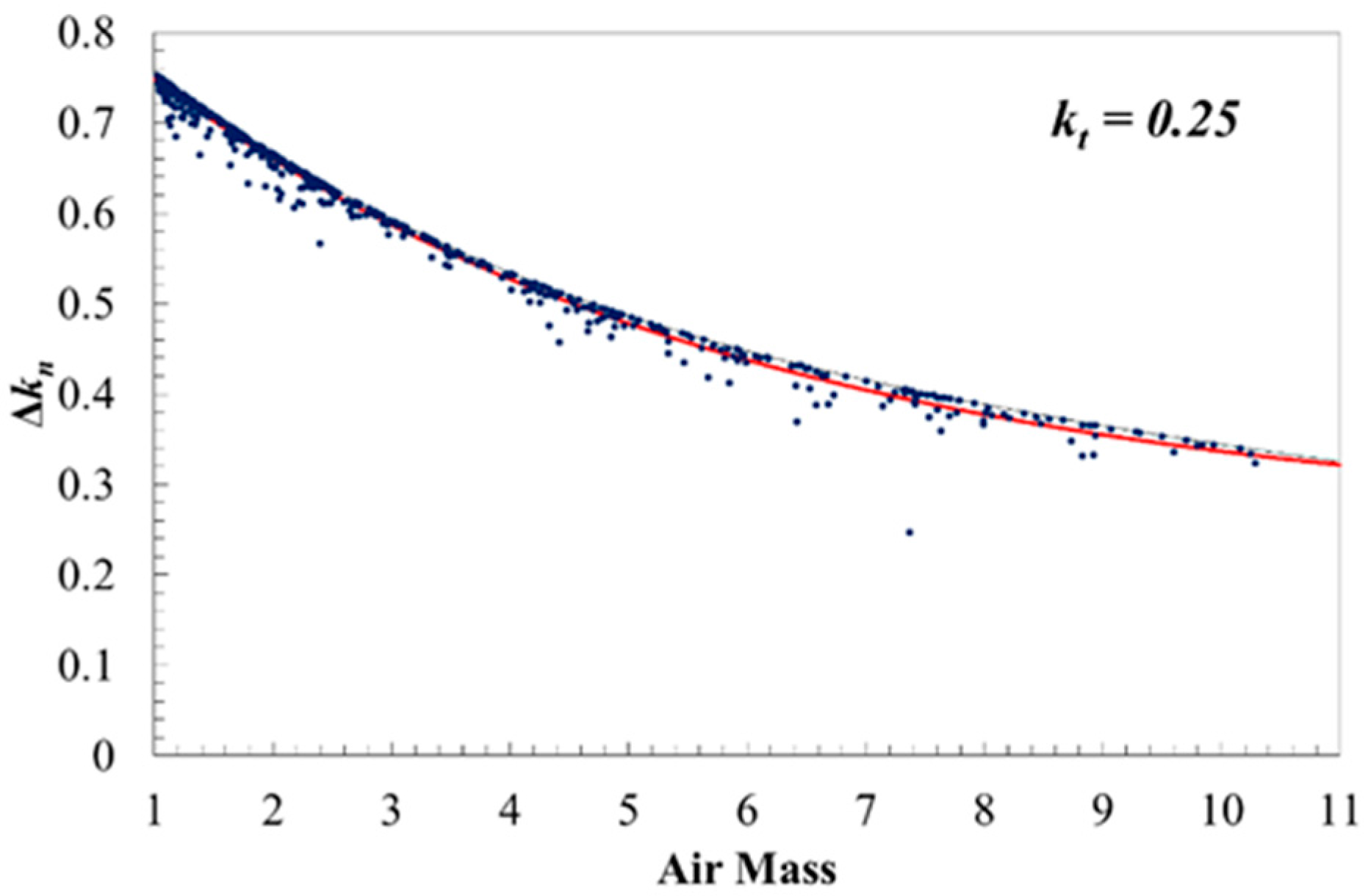
Figure 4.
Regression analysis to fit the coefficients A, B, and C according to Equation (8).
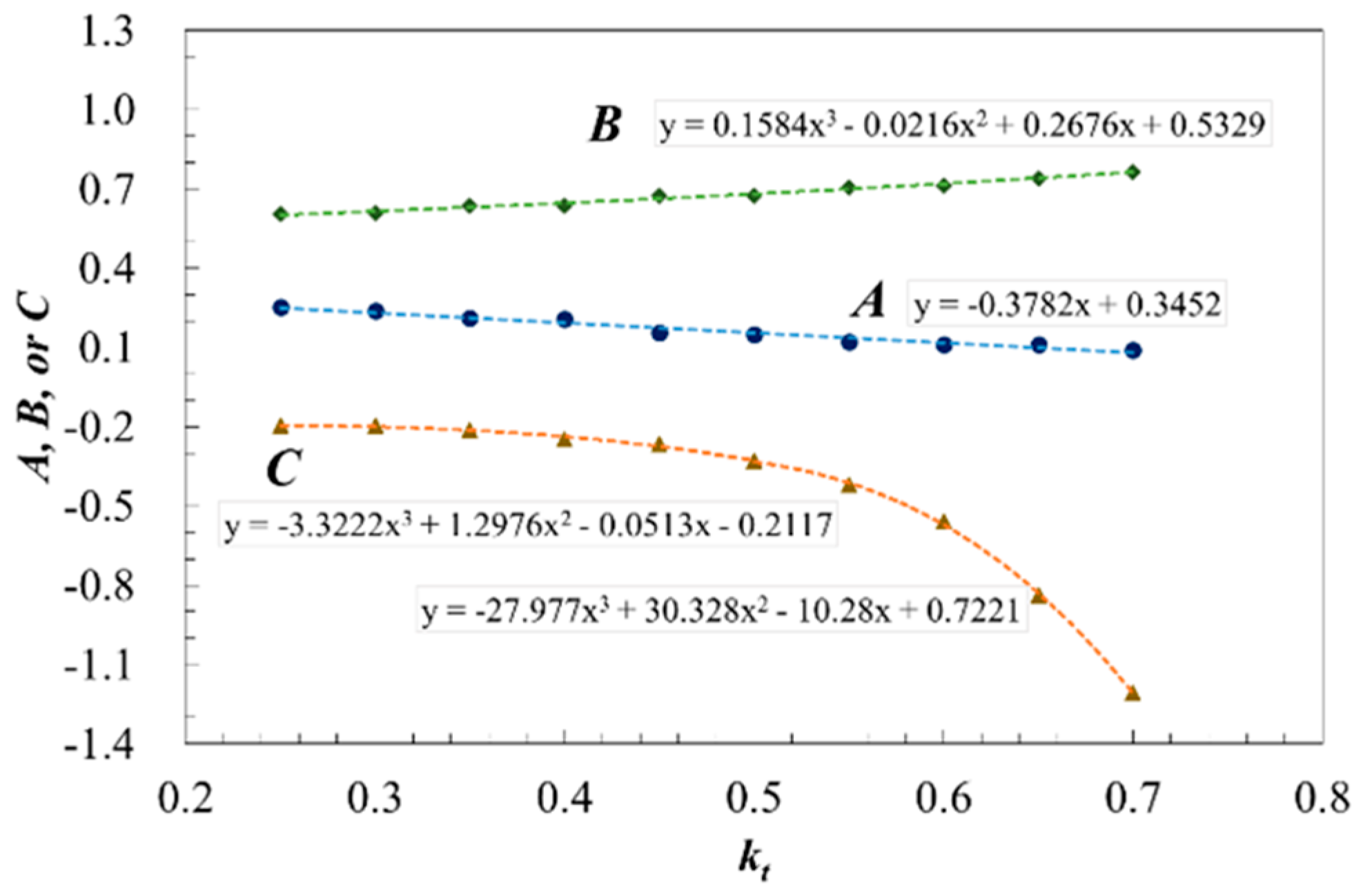
Figure 5.
Scatterplot of the DNI measurement and estimation from the new model.
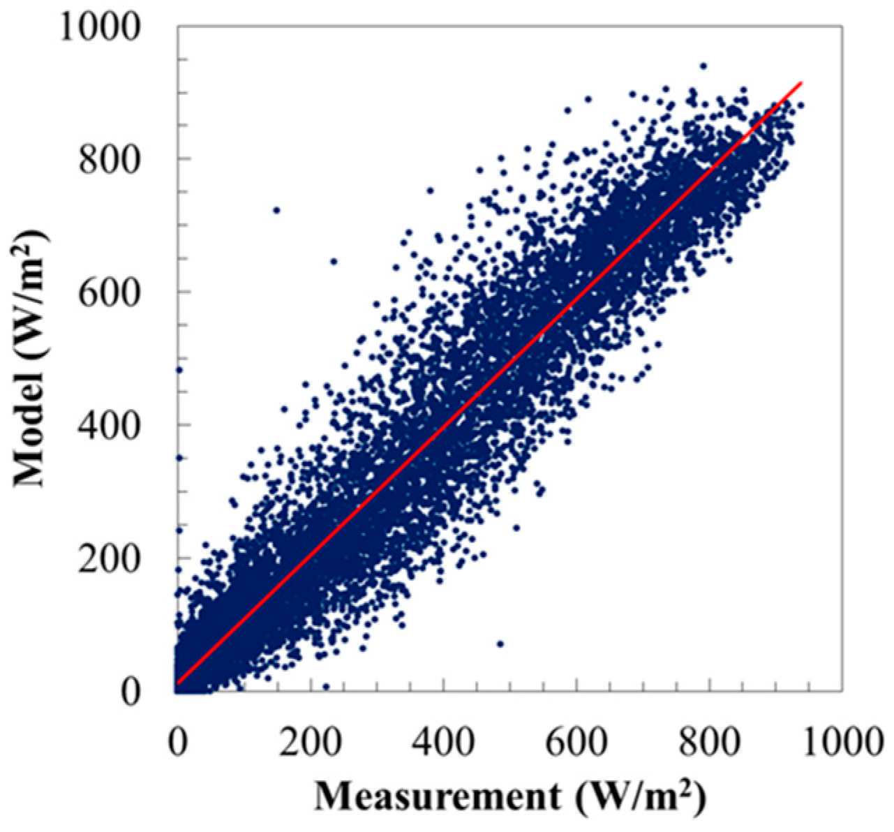
Figure 6.
Relative errors for estimating the monthly sum of the DNI.

Figure 7.
Effects of the solar zenith angle on errors for estimating the hourly DNI, in which the dotted and the solid lines indicate the averages of the Reindl-2 and the new models in each separate interval of the solar zenith angle, respectively: (a) June 2009; and (b) December 2009.
Figure 7.
Effects of the solar zenith angle on errors for estimating the hourly DNI, in which the dotted and the solid lines indicate the averages of the Reindl-2 and the new models in each separate interval of the solar zenith angle, respectively: (a) June 2009; and (b) December 2009.
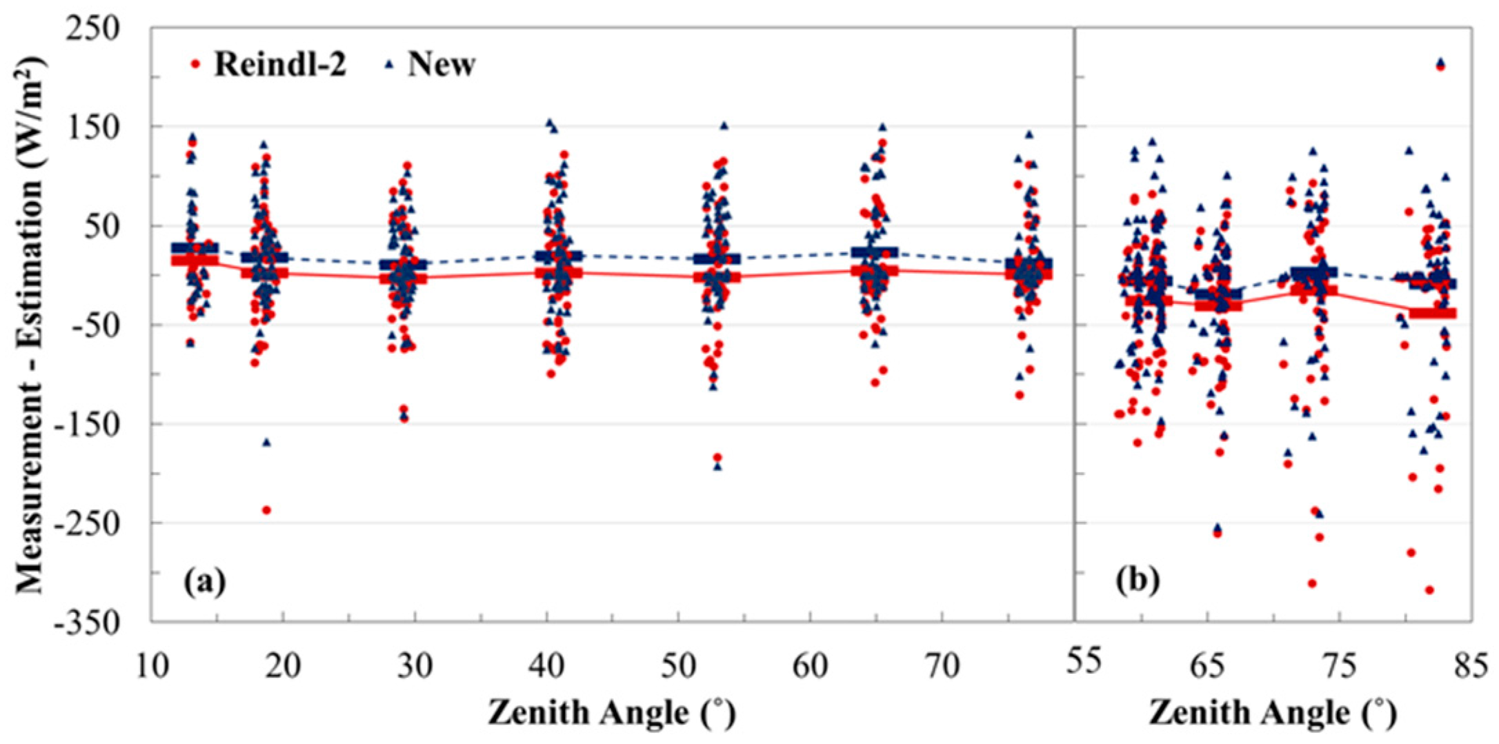
Figure 8.
Yearly sums of the GHI from the long-term mean, in the TMY data from Korean Solar Energy Society (KSES), and in the TMY data generated using the Maxwell, the Reindl-2, and the new models.
Figure 8.
Yearly sums of the GHI from the long-term mean, in the TMY data from Korean Solar Energy Society (KSES), and in the TMY data generated using the Maxwell, the Reindl-2, and the new models.
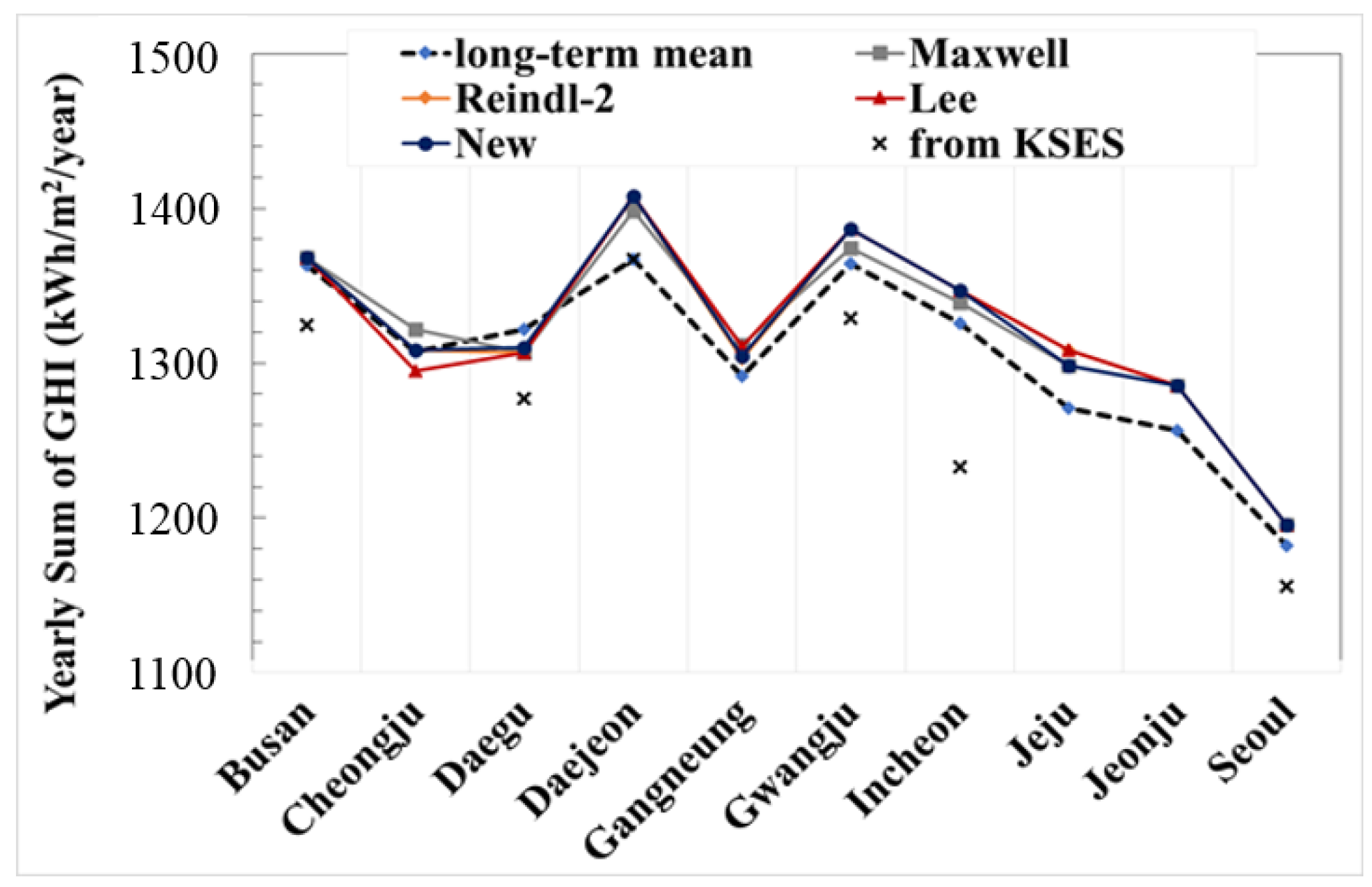
Figure 9.
Yearly sums of the DNI in the TMY data from KSES and in the TMY data generated using the Maxwell, the Reindl-2, and the new models.
Figure 9.
Yearly sums of the DNI in the TMY data from KSES and in the TMY data generated using the Maxwell, the Reindl-2, and the new models.

Table 1.
Regression analysis of each model with a linear polynomial of : the coefficient of determination (R2), the mean bias error (MBE) as the measurement minus estimation, the root mean square error (RMSE), and the median absolute deviation (MAD).
Table 1.
Regression analysis of each model with a linear polynomial of : the coefficient of determination (R2), the mean bias error (MBE) as the measurement minus estimation, the root mean square error (RMSE), and the median absolute deviation (MAD).
| Group | Model | C1 | C0 | R2 | MBE | RMSE | MAD |
|---|---|---|---|---|---|---|---|
| I | Orgill and Hollands [16] | 0.99 | 15.70 | 92.8% | −11.91 | 75.16 | 28.14 |
| Vignola and McDaniels [17] | 0.96 | 30.16 | 92.3% | −19.95 | 78.11 | 32.58 | |
| Louche et al. [18] | 1.06 | 29.33 | 93.0% | −45.45 | 92.02 | 31.70 | |
| Erbs et al. [21] | 1.03 | 12.08 | 92.9% | −20.92 | 80.07 | 29.62 | |
| Reindl et al. [22]—1 | 0.98 | 27.22 | 92.9% | −23.17 | 77.10 | 30.20 | |
| Lam and Li [19] | 0.92 | 60.77 | 91.8% | −39.16 | 86.37 | 37.98 | |
| II | Lee et al. [8] | 0.78 | 42.12 | 92.7% | 16.23 | 85.43 | 37.80 |
| CIBSE [20] | 0.89 | 20.77 | 92.9% | 6.93 | 72.63 | 30.07 | |
| III | Reindl et al. [22]—2 | 0.97 | 26.24 | 93.7% | −17.82 | 70.29 | 26.84 |
| Maxwell [13] | 1.04 | 26.78 | 93.2% | −37.05 | 84.95 | 30.38 | |
| New | 0.96 | 12.16 | 94.5% | −2.04 | 63.37 | 26.57 | |
Table 2.
Relative errors for estimating the yearly sum of the DNI.
| Model | 2007 | 2008 | 2009 |
|---|---|---|---|
| Maxwell | 15.3% | 13.2% | 12.3% |
| Reindl-2 | 7.7% | 5.7% | 5.5% |
| New | 1.5% | −0.1% | −0.5% |
Table 3.
Weighting factors for the Finkelstein-Schafer (FS) statistics.
| Weather Element | Weighting Factor | Weather Element | Weighting Factor |
|---|---|---|---|
| Max Dry Bulb Temperature | 1/20 | Mean Dew Point Temperature | 2/20 |
| Min Dry Bulb Temperature | 1/20 | Max Wind Velocity | 1/20 |
| Mean Dry Bulb Temperature | 2/20 | Mean Wind Velocity | 1/20 |
| Max Dew Point Temperature | 1/20 | Global Horizontal Irradiance | 5/20 |
| Min Dew Point Temperature | 1/20 | Direct Normal Irradiance | 5/20 |
© 2017 by the authors. Licensee MDPI, Basel, Switzerland. This article is an open access article distributed under the terms and conditions of the Creative Commons Attribution (CC BY) license (http://creativecommons.org/licenses/by/4.0/).
Share and Cite
MDPI and ACS Style
Lee, H.-J.; Kim, S.-Y.; Yun, C.-Y. Comparison of Solar Radiation Models to Estimate Direct Normal Irradiance for Korea. Energies 2017, 10, 594. https://doi.org/10.3390/en10050594
AMA Style
Lee H-J, Kim S-Y, Yun C-Y. Comparison of Solar Radiation Models to Estimate Direct Normal Irradiance for Korea. Energies. 2017; 10(5):594. https://doi.org/10.3390/en10050594
Chicago/Turabian StyleLee, Hyun-Jin, Shin-Young Kim, and Chang-Yeol Yun. 2017. "Comparison of Solar Radiation Models to Estimate Direct Normal Irradiance for Korea" Energies 10, no. 5: 594. https://doi.org/10.3390/en10050594
Note that from the first issue of 2016, this journal uses article numbers instead of page numbers. See further details here.