
High-Gain Disturbance Observer-Based Robust Load Frequency Control of Power Systems with Multiple Areas


Department of Electrical and Information Engineering, Seoul National University of Science and Technology, Seoul 01811, Korea
*
Author to whom correspondence should be addressed.
Energies 2017, 10(5), 595; https://doi.org/10.3390/en10050595
Submission received: 28 February 2017
/
Revised: 21 April 2017
/
Accepted: 22 April 2017
/
Published: 29 April 2017
(This article belongs to the Section F: Electrical Engineering)
Abstract
:This paper proposes a high-gain disturbance observer (HDOB)-based controller for load frequency control (LFC) of power systems with multiple areas. The main goal of LFC problem is to maintain the frequency to its nominal value. The objective of this paper is to reject frequency variations due to abrupt load changes and diverse uncertainties (e.g., inertia and damping parameters, and interconnection topology, etc.) by employing the HDOB for the LFC. The simulation results demonstrate the effectiveness of the proposed HDOB-based LFC by showing that it successfully rejects frequency variations owing to load changes and frequency variations occurring in various locations in interconnected power systems. Besides, it is shown that the proposed LFC can eliminate frequency deviations although there are delays in transmission among the power systems with multiple areas.
1. Introduction
Frequency is an important quality index in power systems since it indicates if the balance between the electrical load and the power supplied by generators is maintained. A large frequency deviation can harm equipment, decay load performance, cause the transmission lines to be overloaded, damage protection schemes, and ultimately lead to the frequency instability. Frequency instability is the condition where the system fails to maintain its frequency within a certain operating point. Since frequency is proportional to the rotational speed of the generator, the problem of frequency control may be directly translated into a speed control problem of turbine-generator unit.
Frequency control is constructed by three levels: primary, secondary, and tertiary control. Primary control is provided in all generating units and responds within few seconds. As soon as the imbalance occurs, the governor changes its speed with a certain proportional action. Under normal operation, the primary control can attenuate small frequency deviation, but for larger deviation, secondary control is needed. Since the primary control is nothing but the proportional control from control theoretic point of view, it cannot guarantee the zero-steady state error. Secondary control is provided to steer frequency deviation to zero. Secondary control is commonly referred as load frequency control (LFC). Following a serious situation, if the frequency is quickly dropped to a critical value, tertiary control may be required to restore the nominal frequency.
In this paper, interconnected power systems are considered. Interconnected electric power systems allow utilizing tie-lines to transmit power from one area to another area. Hence any load disruption can cause frequency fluctuation due to change of tie line power deviation. LFC aims to drive frequency deviation and tie line power deviation to zero under unknown load in power systems. The effect of the system frequency due to load power change is described by a swing equation [1]. However, the component of power systems such as generators and loads are dynamic, thus result in uncertain parameters in the swing equation. Hence the LFC has to be able to handle the frequency under this circumstance. The LFC needs to get the frequency from all interconnected areas and its own frequency to determine the proper control effort. Because of transmission distance and filters in measurement devices, the frequency measurements are delayed which may harm the response of the LFC. Therefore, considering the measurement delay is important in designing a proper LFC.
Classical control strategies for the LFC use integral of tracking error as a control signal [1]. However, those methods are incapable of dealing with parameter variations and nonlinearities effectively. Studies on the LFC has been reported using a suboptimal LFC regulator to handle the limitation of power systems observability [2,3]. Various adaptive control techniques are proposed for plant parameter changes in [4,5]. Despite the promising concept of adaptive controllers, the control algorithm is too complicated to implement in large scale systems and can show poor transient performance which can be critical in power systems. Several papers propose an observer for dealing with uncertain load changing in power systems with multiple areas [6,7,8,9,10,11,12,13,14,15,16]. In [6,7,8], a disturbance observer is considered to handle large-scale wind power in power systems. In these applications, the uncertainty and external disturbance are viewed as a total disturbance and rejected by an active disturbance observer proposed by [9,10,11,12,13]. The disturbance is estimated using an extended state observer (ESO) in [15]. However, from [16], higher order ESO is needed to get the perfect estimation. In principle, an exact system model has to be known to design such disturbance observers, which hardly holds in practice due to uncertain parameters (e.g., inertia and damping parameters) in the system.
In this paper, a high-gain disturbance observer (HDOB)-based robust LFC [17] is designed and applied to power systems with multiple areas in order to reject frequency deviations. The HDOB- based LFC consists of two parts: controller for the nominal model and HDOB. The control for the nominal model is designed first under the assumption that there are no uncertainties in the system under consideration. Then, a HDOB is designed to estimate all uncertainties including model uncertainties and external disturbances, and the estimated disturbance is added to the nominal control to reject uncertainties.
For the purpose of showing the effectiveness of the proposed scheme, three simulation results are given. One shows that the proposed HDOB-based LFC can eliminate the frequency deviation induced by load changes taking place at various locations in power systems under uncertainties in the inertia and damping parameters in the swing equation. The second simulation result demonstrates that the proposed LFC can get rid of the frequency deviation despite the measurement delay which can lead to harmful effect in existing approaches. In addition, a severe uncertainty in power systems is that a generator can trip or even one area can be disconnected from the other power systems areas due to severe fault or operational reason. So, it is necessary to investigate robustness of the proposed LFC against such topology changes. Simulation results demonstrate that the HDOB-based LFC indeed shows robustness against topologies in one area power system and between areas.
2. Dynamic Model of Power Systems with Multiple Areas
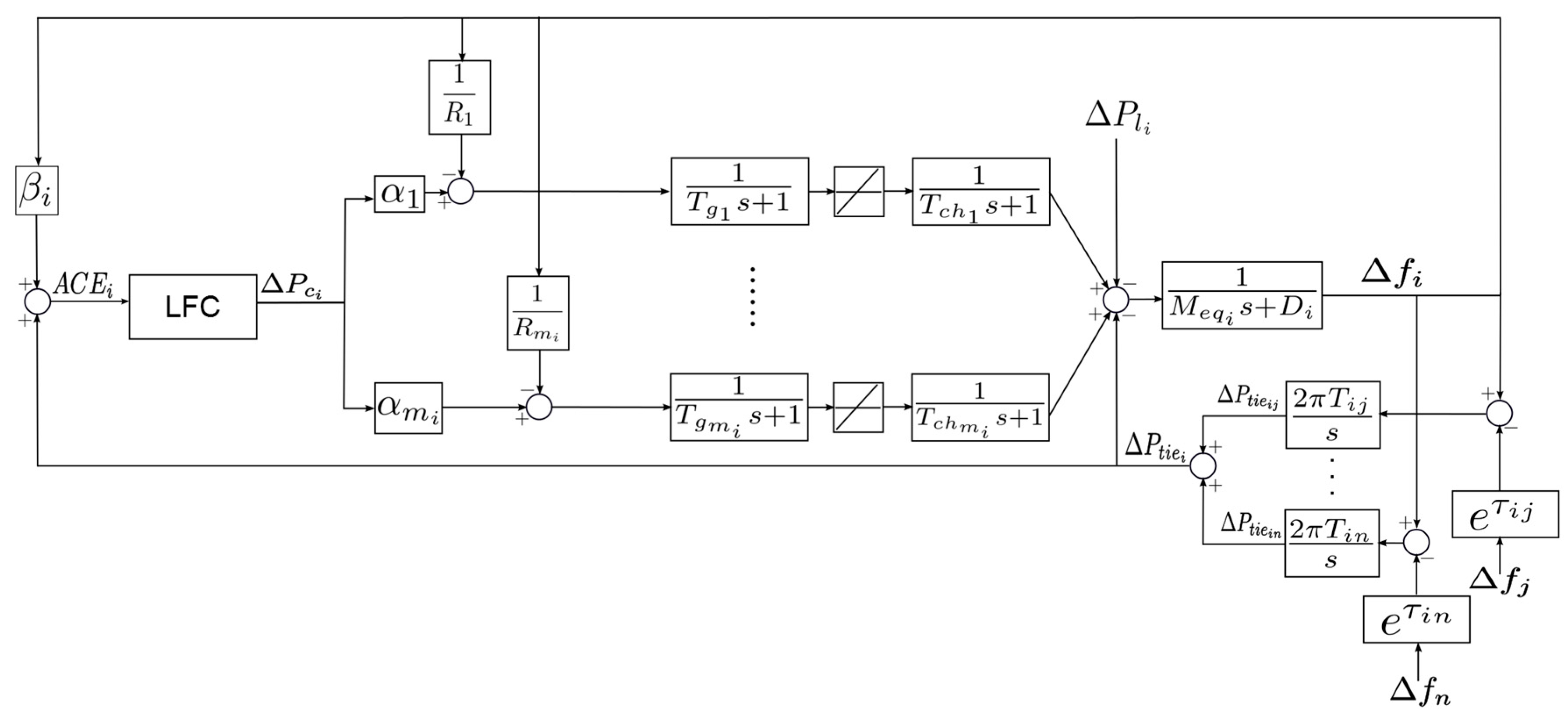
In this section, a mathematical model of power systems with multiple areas for LFC design is introduced [1,11]. A typical power systems with multiple areas is considered in this paper (Figure 1). As shown in Figure 1, each control area has its own load power change Unpredicted fluctuations of load power is treated as a disturbance for the system. Under this circumstance, both primary and secondary controls attempt to remove the frequency deviation in each area. The droop coefficient represents the proportional gain used in the primary control. Furthermore, the objective is to design a secondary control (LFC) to improve the result of the primary control.
From Figure 1, the system is comprised of the generators, as an electrical power generation, and a load. The number of the generators in the th area is denoted as The generator model consists of two major generation units: a governor and a turbine. Both are represented in a first order linearized model. The dynamics of the governor can be expressed as:
and the dynamics of non-reheating turbine unit can be expressed as:
where and are the time constants of the governor and the turbine model in the th generator.
The basis for attaining the regulation function is the tie line bias control concept that is introduced over 50 years ago [18] and widely used to model the power flow between two or more buses [2,3,4,5,6,9,10,11,19,20]. Tie line power deviation is defined as the deviation power exported to the th area and is equal to the sum of all outflowing line power changes in the line that connects to the th area with its neighboring areas:
Tie line power change in the th area corresponding to the th area, is defined as:
where is synchronizing torque coefficient and and are frequency deviation of the th area and the th area. For the purpose of taking the measurement delay from the th area to the th area into account, delay is applied. See in Figure 1.
In this LFC model, strongly connected and synchronized generators are in one area power system. Assuming that all generators have coherent response of load changing, yields an equivalent equation as follows:
where the effects of system loads are lumped into a single damping constant with the summation of inertia constants of all generating units denoted as . Area control error (ACE) is used to obtain power deviation reference. represents the surplus or deficiency of the th area generation and is the summation of tie line power deviation and frequency deviation multiplied by bias factor :
Along with the primary control, the secondary control converts ACE to a command and drives the speed changer of the governing system. Then the speed governing characteristic is shifted to a new set point and results in the matching load demand. Each corresponding generator produces energy based on its constant share control effort αk.
Let generating energy as control input . For connected generators in the th area, frequency deviation can be represented in a function of , load change , and the summation of all frequency deviation from other areas . The function can be written in frequency domain as follows:
where is the constant share effort for the th generator, and are defined as
Hence, the general function of frequency deviation is written as follows:
where:
In this LFC problem, the ACE is considered as the system output . With defined in (10), the output can be expressed as:
where is the Laplace transform of . In (12), and can be treated as one external disturbance . In other words, the th area considers neighboring frequency deviation and power load change as its external disturbance. In view of (12), the input-output relation of the system in the th area can be written as:
where is defined as:
Multiplying right and left side in (13) with yields:
where is a proper transfer function. For the purpose of the controller design, it is desirable to obtain a simplest possible model. To this end, the previous equation can be written as:
where denotes a lumped disturbance and is a parameter. Hence, in the time domain, the model can be expressed as:
where is the inverse Laplace transform of . The corresponding state space model is given by:
where Note that is determined by other parameters, for example, , , and and so on. In general, inertia parameter and damping constant are uncertain. Hence, is uncertain as well but its upper and lower bounds can be known since those of and can be known. This paper pays particular attention to the uncertainties in and . Consequently, the resulting model (18) is a third order uncertain model with unknown bounded external disturbances. As a matter of fact, it is not easy to design an observer due to the uncertain parameter since it is not clear which value is used for in the observer model. Note that representing ACE is the only measurable signal in general.
With the uncertain model in mind, the LFC problem is to design using the measurement such that converges to zero despite uncertain and external disturbance . Note that convergence of to zero implies that the frequency is regulated to its nominal value.
The nominal model of the uncertain model can be assumed as:
where is the controller for the nominal model and denotes the nominal parameter of .
For this nominal model, there are many standard control design methods to regulate the state. For example, pole placement and linear quadratic regulator (LQR) are the representatives of such methods. However, difficulty here is that the original model is uncertain and, in general, the state is not measurable. Hence, the objective of the LFC is to design a robust output feedback stabilizing control for (18). For control design, it is assumed that the lumped disturbance is unknown and bounded. In the next section, a HDOB based robust output feedback control design is presented.
3. Review of HDOB Based Controller
This section briefly reviews the basic concept of the HDOB in [17]. The dynamic system in Figure 1 shows that each control area has different physical parameters and coefficients for the droop control. This makes the problem even more challenging, that the controller should be able to handle the presence of disturbances as well as the parameter uncertainties. Regarding this issues, a HDOB based controller is employed as it is known to be robust against large parameter uncertainties and external disturbances.
The structure of HDOB based controller is described by Figure 2 where is the plant output, and u is the control signal [17]. and are stable low pass filters, is the controller for the nominal model, uncertain dynamic system and is the nominal model given by:
where and denote the uncertain parameters of , the state of the plant , and are known nominal parameters of , the state of the nominal .
Suppose that is the same as . By multiplying plant output y with the inverse of nominal model , we could obtain which is roughly the same as the actual input to the uncertain system, i.e., . The estimated disturbance is obtained by subtracting with filtered control input Low pass filter and are formulated as:
Thus, filtered nominal model can be written in state space as:
where:
with and design parameters, and is the state vector of . With the parameters given earlier, can be expressed as:
where . While the filtered control signal u is defined as that can be written in a state space as:
where is the state vector of with . Consequently, the HDOB estimates the disturbance with:
As shown in Figure 2, the closed-loop system consists of the uncertain system , the nominal controller , and (22)–(27). The proposed HDOB based robust control is given by:
Assumption 1.
All the uncertain parameters in and the unknown external disturbance in (20) are bounded.
Assumption 2.
The stabilizing control for nominal model is given.
Theorem 1.
[17] Suppose that Assumptions 1 and 2 are satisfied. Then, there exists for a given such that the HDOB based control (19) with any results in:
The idea behind the HDOB based control is that the HDOB makes the input-output relation of the combined system of and HDOB almost the same as that of by canceling the estimated disturbance. Hence, the nominal control can stabilize the whole system. Another important feature of the employed HDOB is that the state the , i.e., , is, in fact, the state estimate of the uncertain plant [17,21]. This feature is importantly used in the proposed LFC design.
4. HDOB Based LFC for the th Area
In this section, the proposed HDOB based LFC is presented. In accordance with the design procedure in the previous section, the nominal control is designed first. In order to design the nominal control for the nominal model (18), any state feedback control law can be employed. For example, using pole placement or LQR, we can design as follows:
where are feedback gains and they are determined such that:
![Energies 10 00595 i001]() becomes asymptotically stable. In this paper, the state feedback gain and are determined using LQR method. The performance index is:
where and are weighting matrices. The optimal state feedback control gains are computed by minimizing and given by:
where , and is the solution of the Riccati equation. Since is not measurable, we can use its estimate in the nominal control . Hence, the nominal control is:
becomes asymptotically stable. In this paper, the state feedback gain and are determined using LQR method. The performance index is:
where and are weighting matrices. The optimal state feedback control gains are computed by minimizing and given by:
where , and is the solution of the Riccati equation. Since is not measurable, we can use its estimate in the nominal control . Hence, the nominal control is:

The HDOB can be designed according to the design method explained in the previous section with . Based on these, the proposed HDOB based LFC is given by:
where is the output of the HDOB given in (27) and function designates the saturation function. The saturation function is employed at the output of the HDOB to avoid the peaking phenomenon which means that a very large control value due to a small can make the state of the system very large as well. Since the HDOB designated in this paper is a high-gain observer type, employing such a saturation function is necessary [22,23]. The HDOB consists of two design parameters: and . Since the nominal model is a third order model, the parameter are chosen such that becomes stable. In addition, is determined sufficiently small.
5. Case Study
In this section, the proposed method is tested to validate its performance against the parameter uncertainties and abrupt load changes in three different cases. Since the moment inertia of generators may varies within a certain bounded interval, first the simulations are carried out to confirm the robustness of the proposed controller to handle this uncertainty. Second, measurement delay between interconnected areas are considered with two different load changes: random and large amplitude step load. Third, simulations with different number of interconnected areas and generators are carried out to look into robustness of the proposed LFC against different network topologies of power systems.
5.1. Frequency Control without LFC
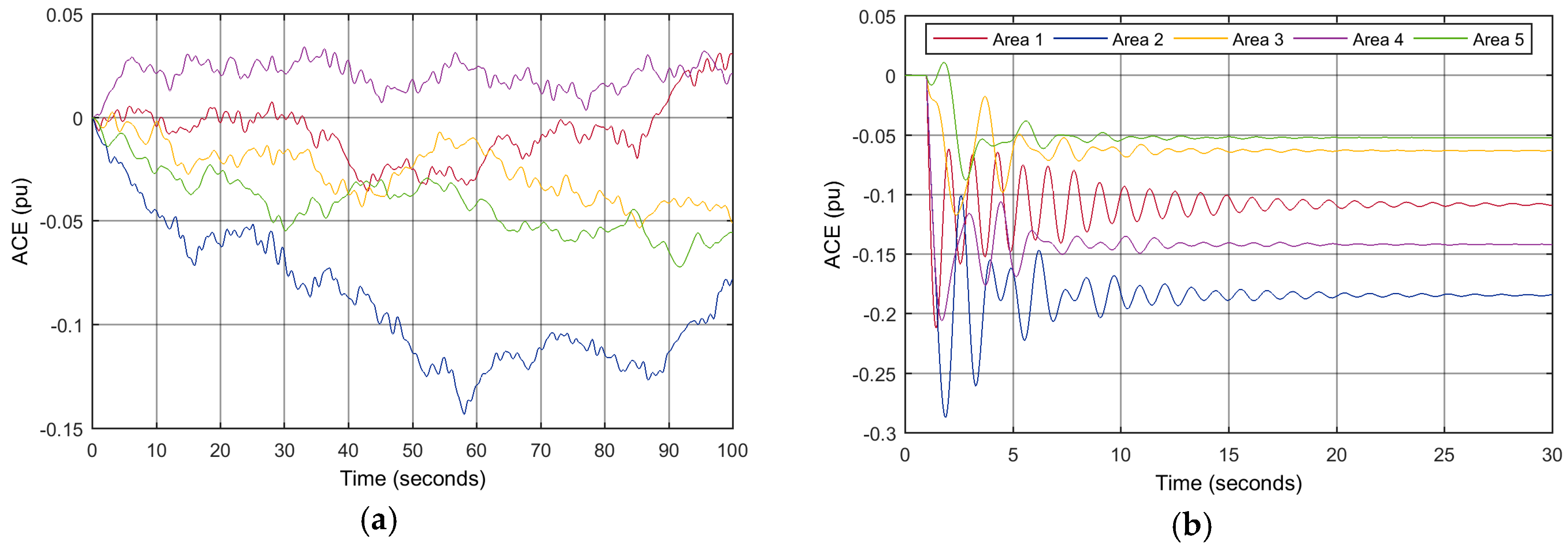
To understand the incompleteness of primary control in handling the frequency problem in interconnected power systems, a simulation without LFC is done. The dynamic model of each area is shown in Figure 1 with its parameters taken from [24] in Table A1. The primary control is employed with two different types of loads. Firstly, random load changes are applied in five-area power systems. The load change variation is chosen between −0.15 p.u. and 0.15 p.u. After that, a large amplitude of step load is added in each area. When small random load variations occur in the system, the primary control can manage the ACE with error 0–0.14 p.u. (Figure 3a). However, from Figure 3b, when a large amplitude of step load is applied, the primary control fails to drive the ACE to zero. Therefore, a LFC is required to achieve the frequency regulation after employing the primary control.
5.2. Robustness against Uncertain Moment of Inertia and Damping Coeficient
The proposed control is tested in the interconnected power system as illustrated in Figure 4. In this network, each area is assumed to have its own LFC. In addition, unlike existing results, the simulation study is conducted under the assumption that each area has different number of generators as follows: , and that and are uncertain but their upper and lower bounds are known which results in uncertain . For simulation, arbitrary values for uncertain and are selected from the intervals in Table A1 and the corresponding is as follows:
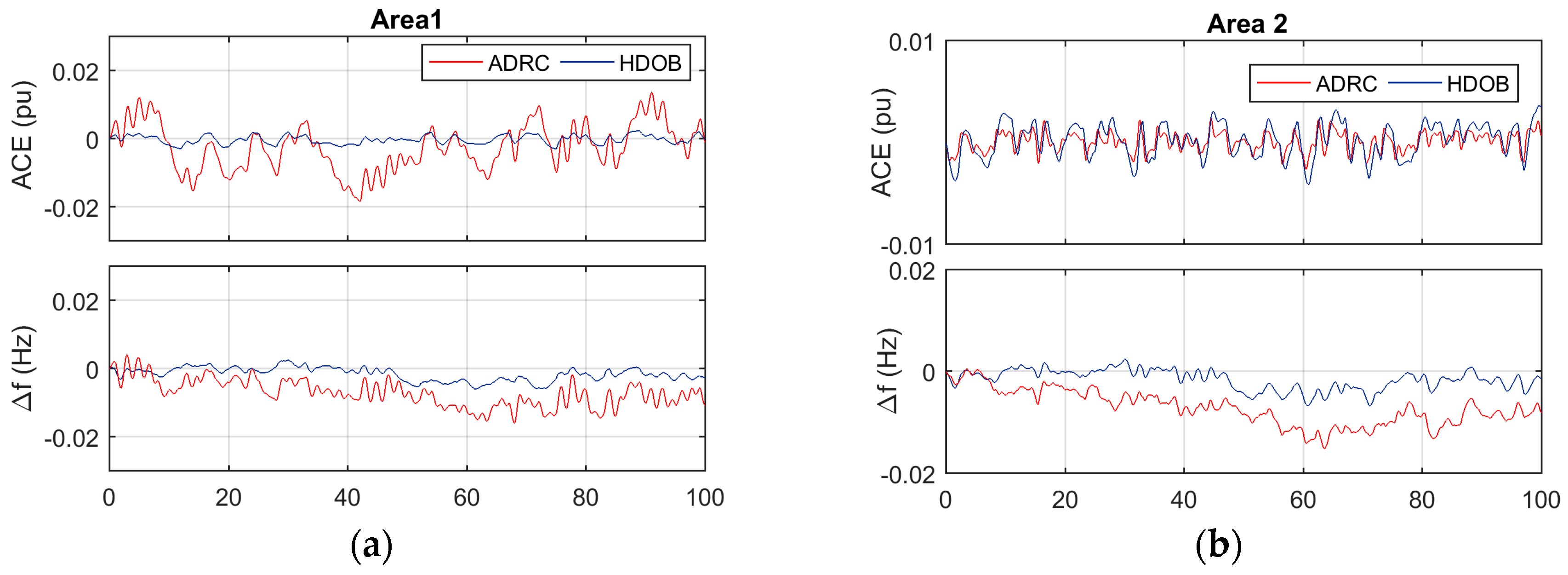
The system is tested with three different load changes: small random, large-amplitude load changes and oscillating load changes. At first, the random loads in Figure 5 are applied and compared with the active disturbance rejection control (ADRC) from [11]. As can be seen in Figure 6, both controllers successfully manage the ACE with the presence of random loads and uncertain parameters in the swing equation. However, in Area 1, 3 and 4, the HDOB has less ACE and compared to the ADRC. Even though in Area 2 and Area 5 the HDOB generates the same ACE as the ADRC, but the HDOB produces smaller than the ADRC in these areas.
In the second case, a large amplitude of step load change is applied to each area at s. For this purpose, the following load changes are used with nominal power .
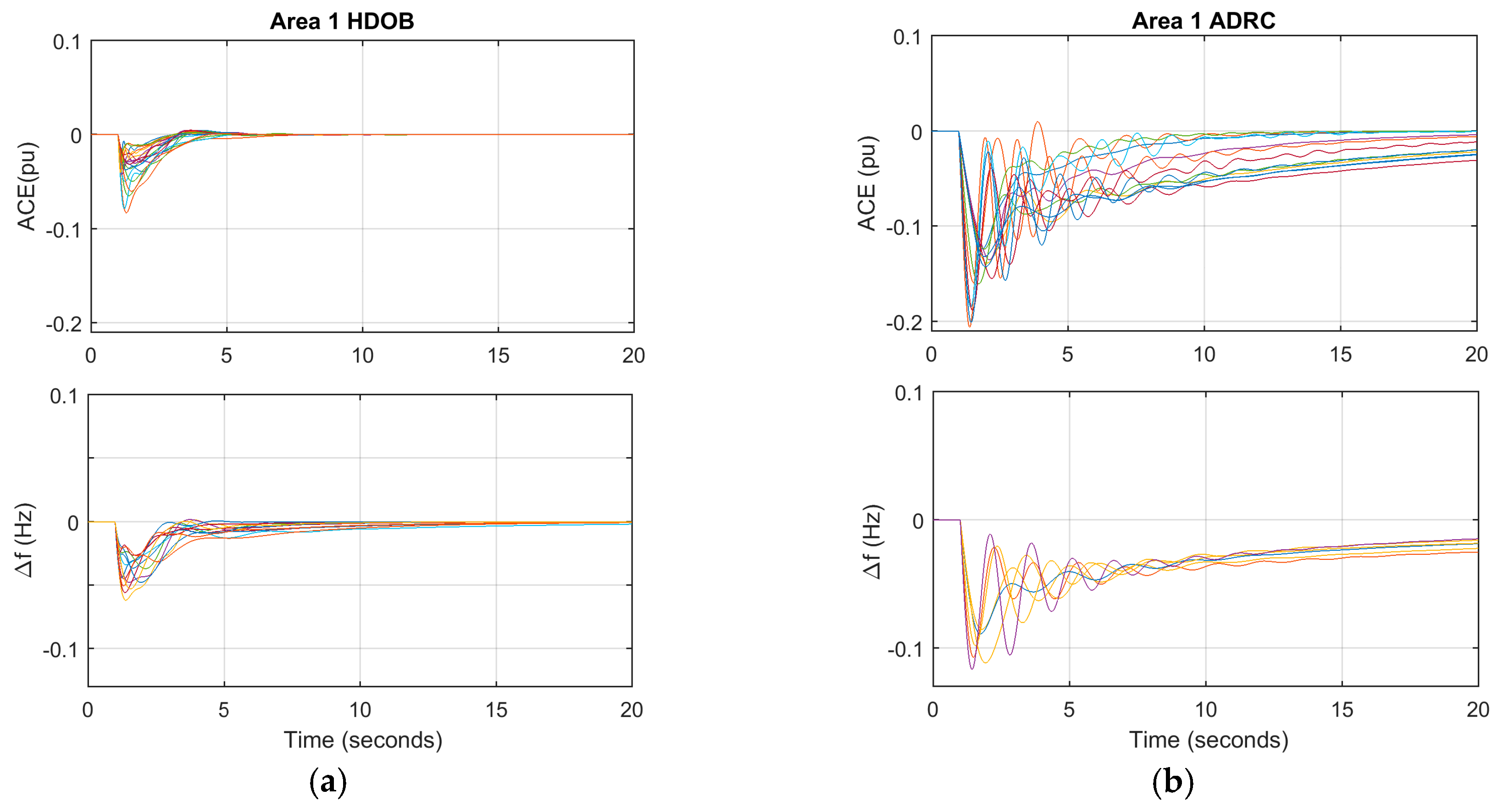
In order to investigate the robustness, the simulations are run 200 times and different and are chosen randomly from the intervals in each simulation. The responses due to different parameters are shown in Figure 7, Figure 8, Figure 9, Figure 10 and Figure 11 for Area 1–5.
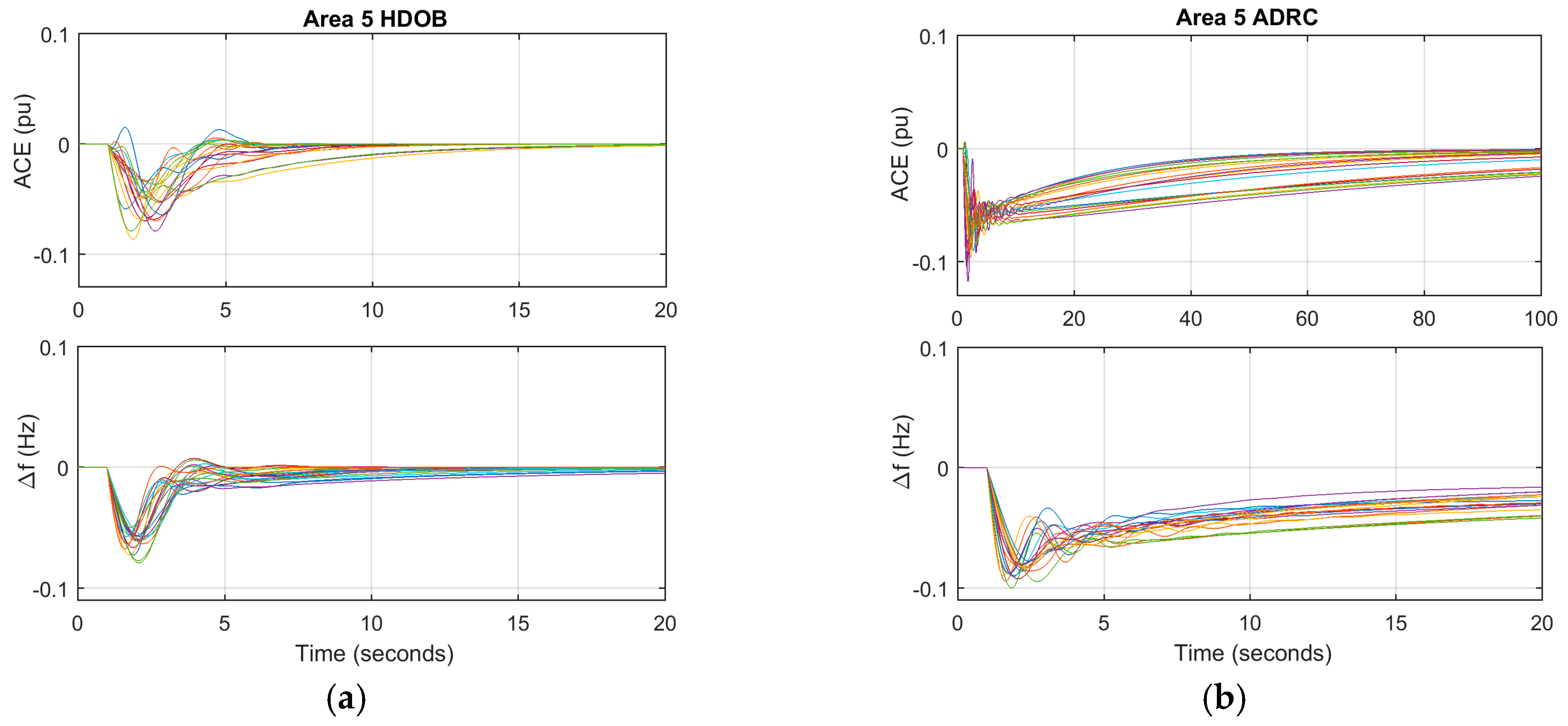
The results are also compared with responses by ADRC and shows the HDOB yields less error in ACE and in transient time and faster responses. In the third case, oscillating disturbances are added to each control area to ensure the stability under the presence of oscillating disturbances from electromagnetic power converters. The disturbances are presented in Figure 12, and the simulation results are presented in Figure 13. As shown in the results, the HDOB successfully eliminates the oscillating disturbances and performs better than the ADRC.
5.3. Robustness against the Delay
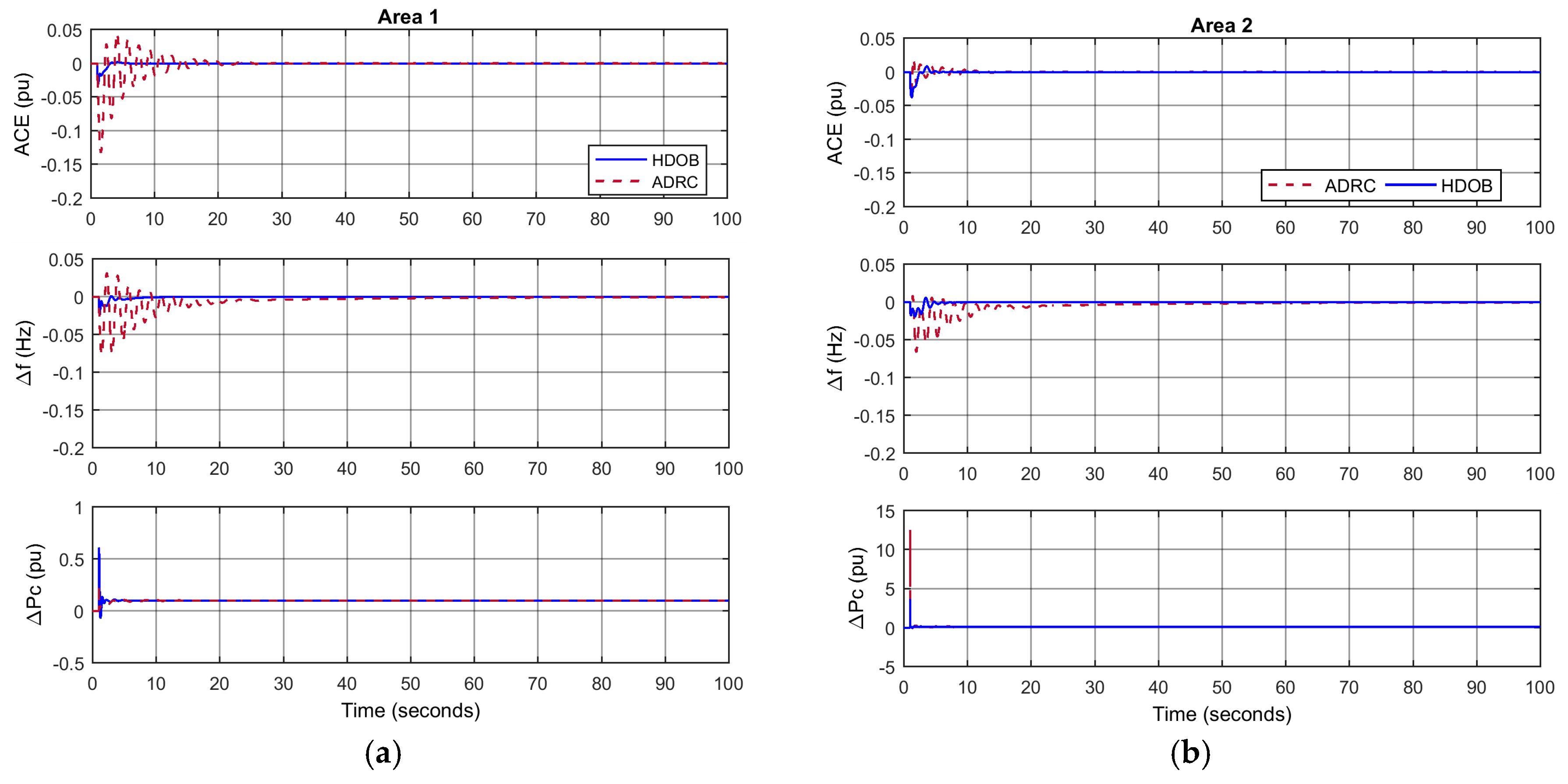
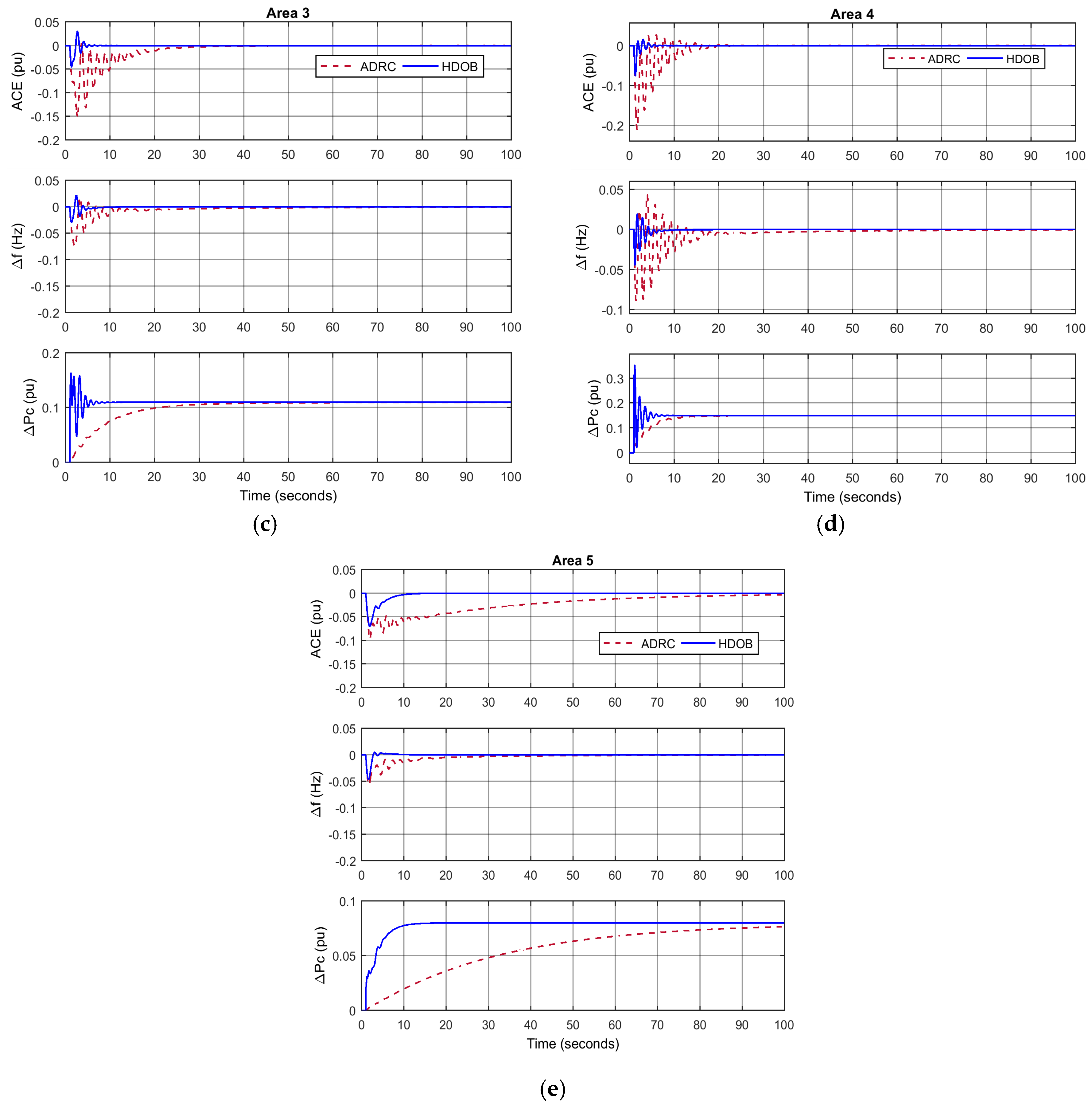
In this scenario, the measurement delays between interconnected areas are taken into account. The delay is chosen as 0.5 s with the random and step load changes as the previous simulation are used. Again, uncertain parameters for and used in the previous simulation are also applied in this simulation. One simulation result is presented in Figure 14 for random load changes, and Figure 15 for step load changes. As a matter of fact, over 200 simulations, quite similar results are obtained. Figure 14 and Figure 15 indicate that both controllers drive the ACE to zero in despite of the delay. However, the proposed HDOB based LFC produces less frequency deviation and faster response than the ADRC. Hence, the HDOB has better performance in dealing with measurement delay under both load variations. See Table A3 in Appendix A for quantitative values of frequency deviation.
5.4. Robustness against Power Systems Topology
This section covers about the performance of LFC in various power system topology. As can be seen in the dynamic system illustrated in Figure 1, the topology can be varying in the number of generators and number of interconnected areas. Hence the interest is to know the effect of LFC responses in terms of different number of generators and number of interconnected areas. Furthermore, it is also important to confirm the capability of the proposed method in different power system topology. The effect of and number of interconnected areas are studied separately and compare with the response of ADRC. The of and are chosen as parameters simulations.
5.4.1. Robustness against Different Number of Generators
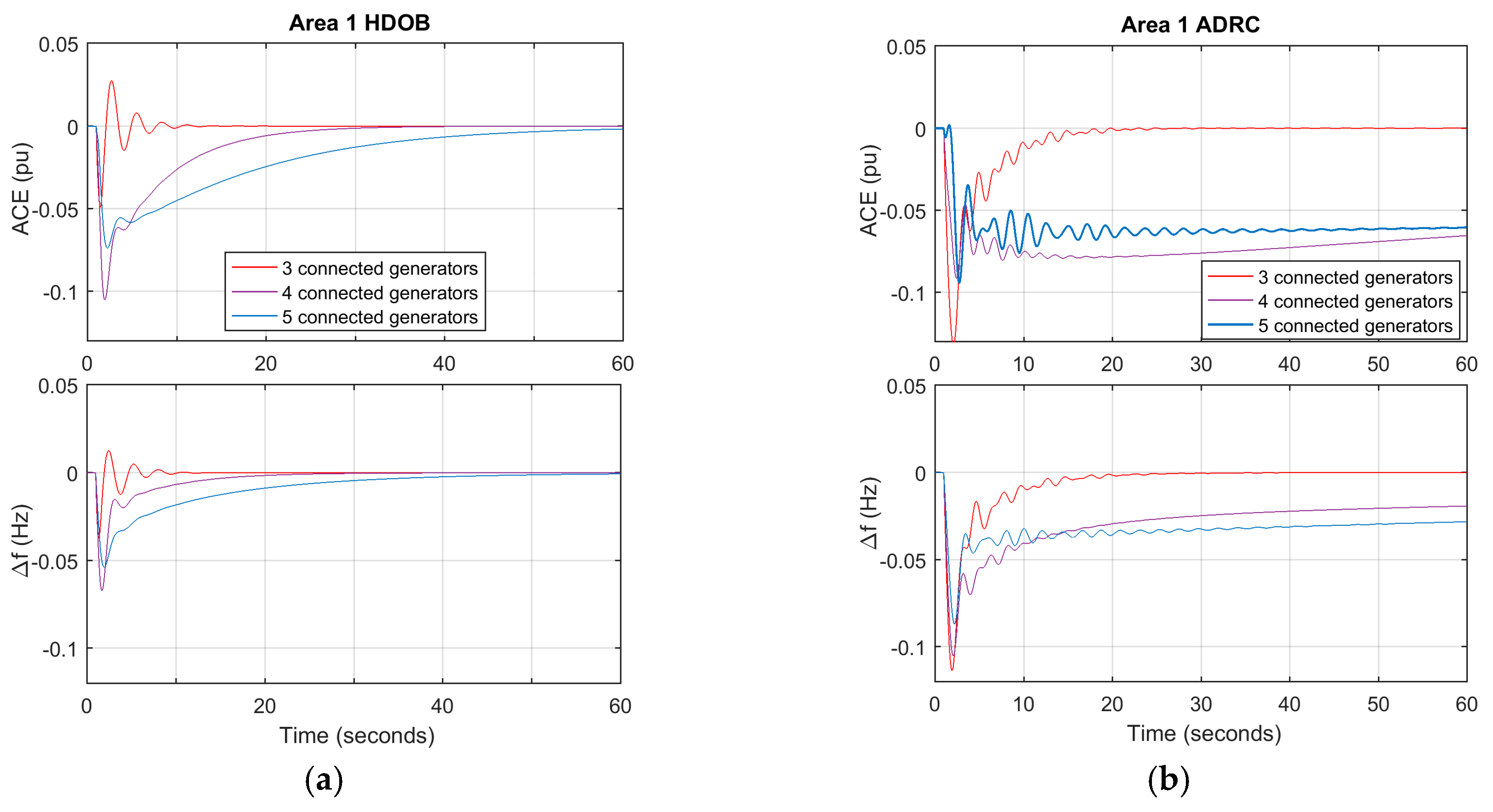
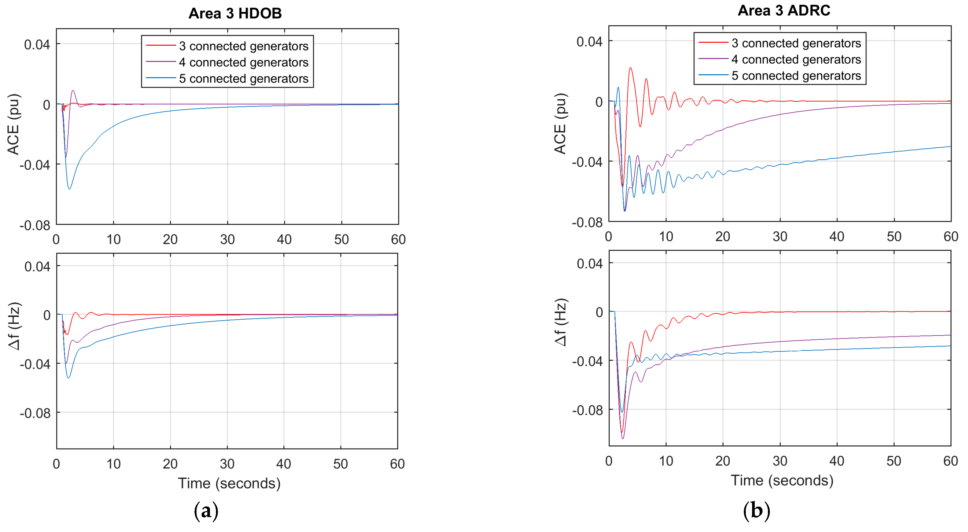
At first the simulation is conducted to know the effect of the controller with changing . The different topologies as shown in Figure 16 are used. The responses after applying 105 MW step load changes in s are compared with ADRC and presented in Figure 17 and Figure 18. Clearly the performances of both controllers are getting degraded as increases. However, the HDOB has better performance regardless of the value of .
5.4.2. Robustness against Different Number of Connected Areas
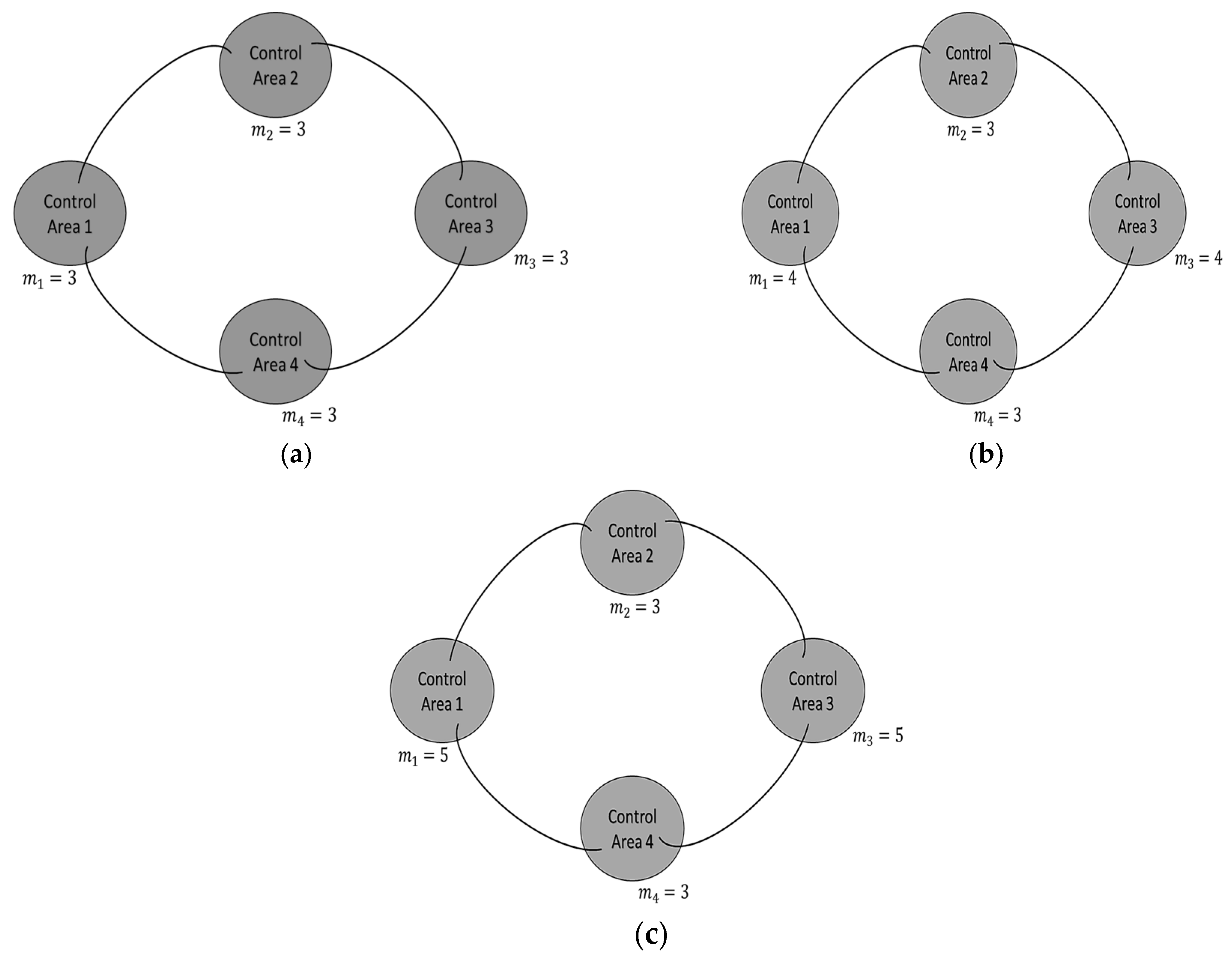
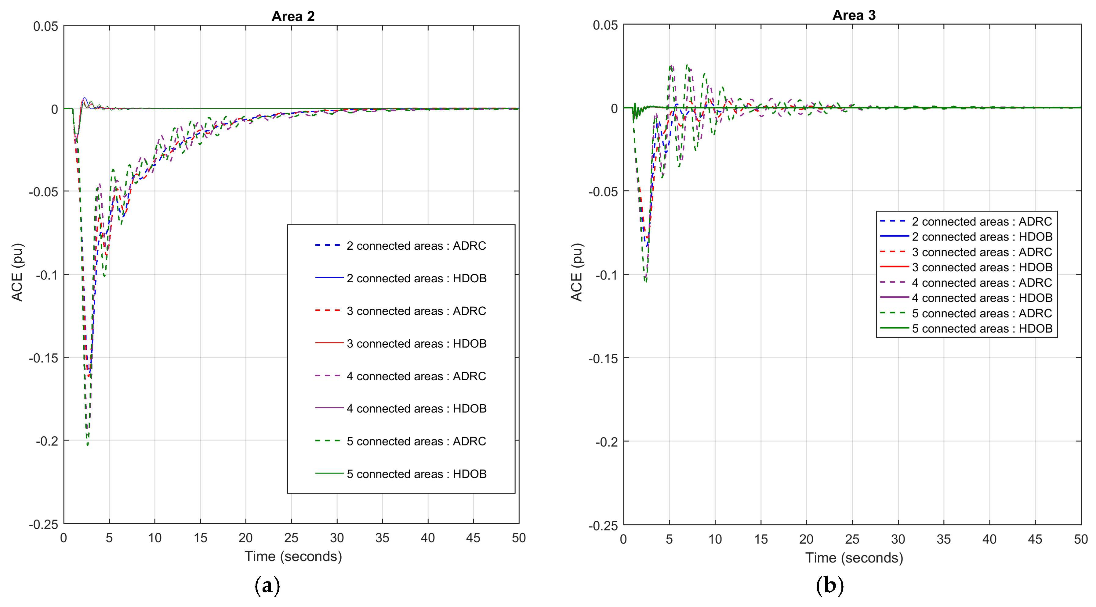
In this scenario, the network topologies as shown in Figure 19 are considered. First, the study starts with two connected areas in Area 2 and Area 3 (Figure 19a), then the number of connected areas is increased by one and it is continued until Area 2 and 3 are connected to five areas (Figure 19d). For the sake of convenience, the number of connected areas in Area 2 is denoted by , and for Area 3, respectively. The simulations are carried out to study the effect of LFC with increasing . In addition, it is also important to confirm the robustness of the designed LFC in different topology. The responses after applying 105 MW step load changes at s are depicted in Figure 20. As can be seen, the proposed HDOB based LFC shows consistent performance in regulating ACE (the solid lines) with the changing . On the contrary, in ADRC results, increasing by two or three decreases the ACE by 0.05 p.u. and makes the overshoot larger (see the dashed lines).
6. Conclusions
In this paper, LFC for power systems with multiple areas using the HDOB is designed. With the load changing tested in the system, the HDOB-based LFC suppresses maximum deviation in frequency and maintains the tie line power interchanges. The advantage of the HDOB-based LFC over existing results is that it reduces frequency deviations robustly in the presence of parameter uncertainties and transmission delay. In addition, it successfully eliminates the frequency deviation under topology variations of multiple areas.
Acknowledgments
This research was supported by Basic Science Research Program through the National Research Foundation of Korea (NRF) funded by the Ministry of Education (NRF-2015R1D1A1A01060588) and by the Human Resources Development of the Korea Institute of Energy Technology Evaluation and Planning (KETEP) grant funded by the Korea government Ministry of Trade, Industry & Energy (20154030200720).
Author Contributions
Jung-Su Kim and Hwachang Song conceived and designed the research problem; and Ismi Rosyiana Fitri performed the simulations and wrote the paper.
Conflicts of Interest
The authors declare no conflict of interest.
Appendix A
The parameters of generators and the proposed LFC are shown in the following tables (Table A1 and Table A2).

Table A1.
Parameters of power systems with multiple areas. (In the case of and , their upper and lower bounds are written).
Table A1.
Parameters of power systems with multiple areas. (In the case of and , their upper and lower bounds are written).
| Generating Unit Parameters | Area 1 | Area 2 | Area 3 | Area 4 | Area 5 |
|---|---|---|---|---|---|
| 3 | 2 | 4 | 3 | 3 | |
| 0.08; 0.06; 0.07 | 0.06; 0.06 | 0.075; 0.08; 0.06; 0.08 | 0.08; 0.06; 0.07 | 0.082; 0.065; 0.063 | |
| 0.4; 0.36; 0.42 | 0.44; 0.32 | 0.44; 0.45; 0.32; 0.40 | 0.43; 0.36; 0.41 | 0.45; 0.33; 0.42 | |
| 3; 3; 3.3 | 3.2273; 2.6667 | 3.54; 3.7; 3.6667; 3 | 3.1; 2.8; 3.01 | 2.9; 2.4; 3.22 | |
| 8; 8; 4 | 12;8 | 8; 8; 8; 8 | 8; 8; 9 | 8; 8; 9 | |
| 0.4; 0.3; 0.3 | 0.4; 0.6 | 0.2; 0.2; 0.3; 0.3 | 0.3; 0.5; 0.2 | 0.3; 0.3; 0.4 | |
| β | 1.0753 | 1.4902 | 0.922 | 1.0321 | 0.9718 |
| 0.0150 × [0.7 1.3] | 0.0140 × [0.7 1.3] | 0.0150 × [0.7 1.3] | 0.0160 × [0.7 1.3] | 0.0130 × [0.7 1.3] | |
| 0.4867 × [0.7 1.3] | 0.3517 × [0.7 1.3] | 1.006 × [0.7 1.3] | 0.557 × [0.7 1.3] | 0.45 × [0.7 1.3] |
Table A2.
Parameters of HDOB and LQR.
| Parameters | Area 1 | Area 2 | Area 3 | Area 4 | Area 5 |
|---|---|---|---|---|---|
| 0.003 | |||||
| saturation level | 20 | ||||
Table A3.
.
| Figure Number | Area 1 | Area 2 | Area 3 | Area 4 | Area 5 | |||||
|---|---|---|---|---|---|---|---|---|---|---|
| ADRC | HDOB | ADRC | HDOB | ADRC | HDOB | ADRC | HDOB | ADRC | HDOB | |
| 6 | −0.007 | −0.001 | −0.007 | −0.001 | −0.007 | −0.001 | −0.007 | −0.001 | −0.007 | −0.002 |
| 7–11 | −0.009 | −7 × 10⁻⁴ | −0.011 | −0.001 | −0.013 | −0.001 | −0.014 | −0.003 | −0.014 | −0.002 |
| 13 | 0.004 | 1.0 × 10⁻⁴ | 0.004 | 1.0 × 10⁻⁴ | 0.004 | 1.0 × 10⁻⁴ | 0.004 | 1.1 × 10⁻⁴ | 0.004 | 9.2 × 10⁻⁵ |
| 14 | −0.001 | −2.9 × 10⁻⁵ | 2.9 × 10⁻⁵ | 3.2 × 10⁻⁵ | 0.0078 | 7.5 × 10⁻⁵ | −9.5 × 10⁻⁴ | −4.9 × 10⁻⁶ | −0.007 | −4.8 × 10⁻⁴ |
| 15 | −0.004 | −3.3 × 10⁻⁴ | −0.004 | −3.3 × 10⁻⁴ | −0.004 | −3.3 × 10⁻⁴ | −0.003 | −3.3 × 10⁻⁴ | −0.004 | −3.3 × 10⁻⁴ |
References
- Kundur, P.; Balu, N.J.; Lauby, M.G. Power System Stability and Control; The EPRI Power System Engineering Series; McGraw-Hill: New York, NY, USA, 1994; pp. 581–623. [Google Scholar]
- Aldeen, M.; Trinh, H. Load-frequency control of interconnected power systems via constrained feedback control schemes. Comput. Electr. Eng. 1994, 20, 71–88. [Google Scholar] [CrossRef]
- Choi, S.S.; Sim, H.K.; Tan, K.S. Load frequency control via constant limited-state feedback. Electr. Power Syst. Res. 1981, 4, 265–269. [Google Scholar] [CrossRef]
- Vajk, I.; Vajta, M.; Keviczky, L.; Haber, R.; Hetthéssy, J.; Kovács, K. Adaptive load-frequency control of the hungarian power system. Automatica 1985, 21, 129–137. [Google Scholar] [CrossRef]
- Lee, K.A.; Yee, H.; Teo, C.Y. Self-tuning algorithm for automatic generation control in an interconnected power system. Electr. Power Syst. Res. 1991, 20, 157–165. [Google Scholar] [CrossRef]
- Shibasaki, S.; Onishi, H.; Iwamoto, S. A study on load frequency control combining a PID controller and a disturbance observer. Proceedings of 2009 Transmission & Distribution Conference & Exposition: Asia and Pacific, Seoul, Korea, 26–30 October 2009. [Google Scholar]
- Kurita, Y.; Moriya, Y.; Iwamoto, S. Control of storage batteries using a disturbance observer in load frequency control for large wind power penetration. In Proceedings of the 2015 IEEE Power Energy Society General Meeting, Denver, CO, USA, 26–30 July 2015. [Google Scholar]
- Abe, K.; Ohba, S.; Iwamoto, S. New load frequency control method suitable for large penetration of wind power generations. In Proceedings of the 2006 IEEE Power Engineering Society General Meeting, Montreal, QC, Canada, 18–22 June 2006. [Google Scholar]
- Liu, F.; Li, Y.; Cao, Y.; She, J.; Wu, M. A two-layer active disturbance rejection controller design for load frequency control of interconnected power system. IEEE Trans. Power Syst. 2016, 31, 3320–3321. [Google Scholar] [CrossRef]
- Tan, W.; Hao, Y.; Li, D. Load frequency control in deregulated environments via active disturbance rejection. Int. J. Electr. Power Energy Syst. 2015, 66, 166–177. [Google Scholar] [CrossRef]
- Dong, L.; Zhang, Y.; Gao, Z. A robust decentralized load frequency controller for interconnected power systems. ISA Trans. 2012, 51, 410–419. [Google Scholar] [CrossRef] [PubMed]
- Fernando, T.; Emami, K.; Yu, S.; Iu, H.H.C.; Wong, K.P. A novel quasi-decentralized functional observer approach to LFC of interconnected power systems. IEEE Trans. Power Syst. 2016, 31, 3139–3151. [Google Scholar] [CrossRef]
- Trinh, H.; Fernando, T.; Iu, H.H.C.; Wong, K.P. Quasi-decentralized functional observers for the LFC of interconnected power systems. IEEE Trans. Power Syst. 2013, 28, 3513–3514. [Google Scholar] [CrossRef]
- She, J.H.; Fang, M.; Ohyama, Y.; Hashimoto, H.; Wu, M. Improving disturbance-rejection performance based on an equivalent-input-disturbance approach. IEEE Trans. Ind. Electron. 2008, 55, 380–389. [Google Scholar] [CrossRef]
- Yang, X.; Huang, Y. Capabilities of extended state observer for estimating uncertainties. In Proceedings of the 2009 American Control Conference, St. Louis, MO, USA, 10–12 June 2009. [Google Scholar]
- Godbole, A.A.; Kolhe, J.P.; Talole, S.E. Performance analysis of generalized extended state observer in tackling sinusoidal disturbances. IEEE Trans. Control Syst. Technol. 2013, 21, 2212–2223. [Google Scholar] [CrossRef]
- Back, J.; Shim, H. Adding robustness to nominal output-feedback controllers for uncertain nonlinear systems: A nonlinear version of disturbance observer. Automatica 2008, 44, 2528–2537. [Google Scholar] [CrossRef]
- Cohn, N. Some aspects of tie-line bias control on interconnected power systems. Trans. Am. Inst. Electr. Eng. Part III Power Appar. Syst. 1956, 75, 1415–1436. [Google Scholar]
- Franzè, G.; Tedesco, F. Constrained load/frequency control problems in networked multi-area power systems. J. Frankl. Inst. 2011, 348, 832–852. [Google Scholar] [CrossRef]
- Tedesco, F.; Casavola, A. Fault-tolerant distributed load/frequency supervisory strategies for networked multi-area microgrids. Int. J. Robust Nonlinear Control 2014, 24, 1380–1402. [Google Scholar] [CrossRef]
- Back, J.; Kim, J.-S. A disturbance observer based practical coordinated tracking controller for uncertain heterogeneous multi-agent systems. Int. J. Robust Nonlinear Control 2015, 25, 2254–2278. [Google Scholar] [CrossRef]
- Khalil, H.K. Nonlinear Systems, 3rd ed.; Prentice Hall: Upper Saddle River, NJ, USA, 2002. [Google Scholar]
- Khalil, H.K. High-gain observers in nonlinear feedback control. In Proceedings of the 2009 IEEE International Conference on Control and Automation, Christchurch, New Zealand, 9–10 December 2009. [Google Scholar]
- Rerkpreedapong, D.; Hasanovic, A.; Feliachi, A. Robust load frequency control using genetic algorithms and linear matrix inequalities. IEEE Trans. Power Syst. 2003, 18, 855–861. [Google Scholar] [CrossRef]
Figure 1.
The dynamic system of th area.

Figure 2.
The block diagram of the HDOB based controller.
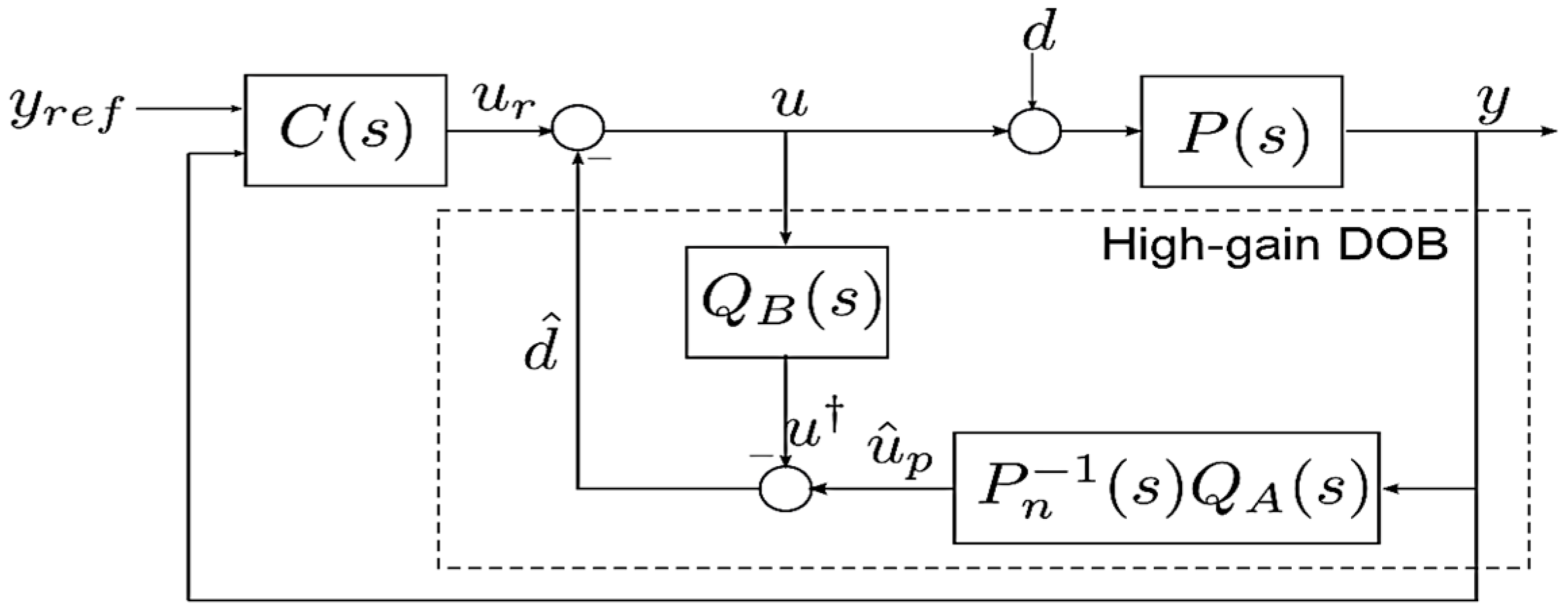
Figure 3.
Area control error (ACE) without applying load frequency control (LFC): (a) With small random load changes; (b) With large amplitude of load changes. pu: p.u.
Figure 3.
Area control error (ACE) without applying load frequency control (LFC): (a) With small random load changes; (b) With large amplitude of load changes. pu: p.u.

Figure 4.
Power systems with multiple area. : number of generators in the area .

Figure 5.
Random load changes applied to the systems.
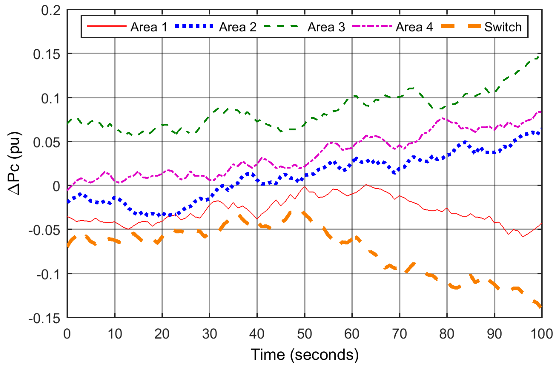
Figure 6.
ACE and of the high-gain disturbance observer (HDOB) and active disturbance rejection control (ADRC) based LFC with large small random load changes and uncertain and in: (a) Area 1; (b) Area 2; (c) Area 3; (d) Area 4; and (e) Area 5.
Figure 6.
ACE and of the high-gain disturbance observer (HDOB) and active disturbance rejection control (ADRC) based LFC with large small random load changes and uncertain and in: (a) Area 1; (b) Area 2; (c) Area 3; (d) Area 4; and (e) Area 5.


Figure 7.
Various response of LFC due to uncertain and in Area 1 with: (a) HDOB; (b) ADRC; after applying large-magnitude step load changes.
Figure 7.
Various response of LFC due to uncertain and in Area 1 with: (a) HDOB; (b) ADRC; after applying large-magnitude step load changes.

Figure 8.
Various response of LFC due to uncertain and in Area 2 with: (a) HDOB; (b) ADRC; after applying large-magnitude step load changes.
Figure 8.
Various response of LFC due to uncertain and in Area 2 with: (a) HDOB; (b) ADRC; after applying large-magnitude step load changes.
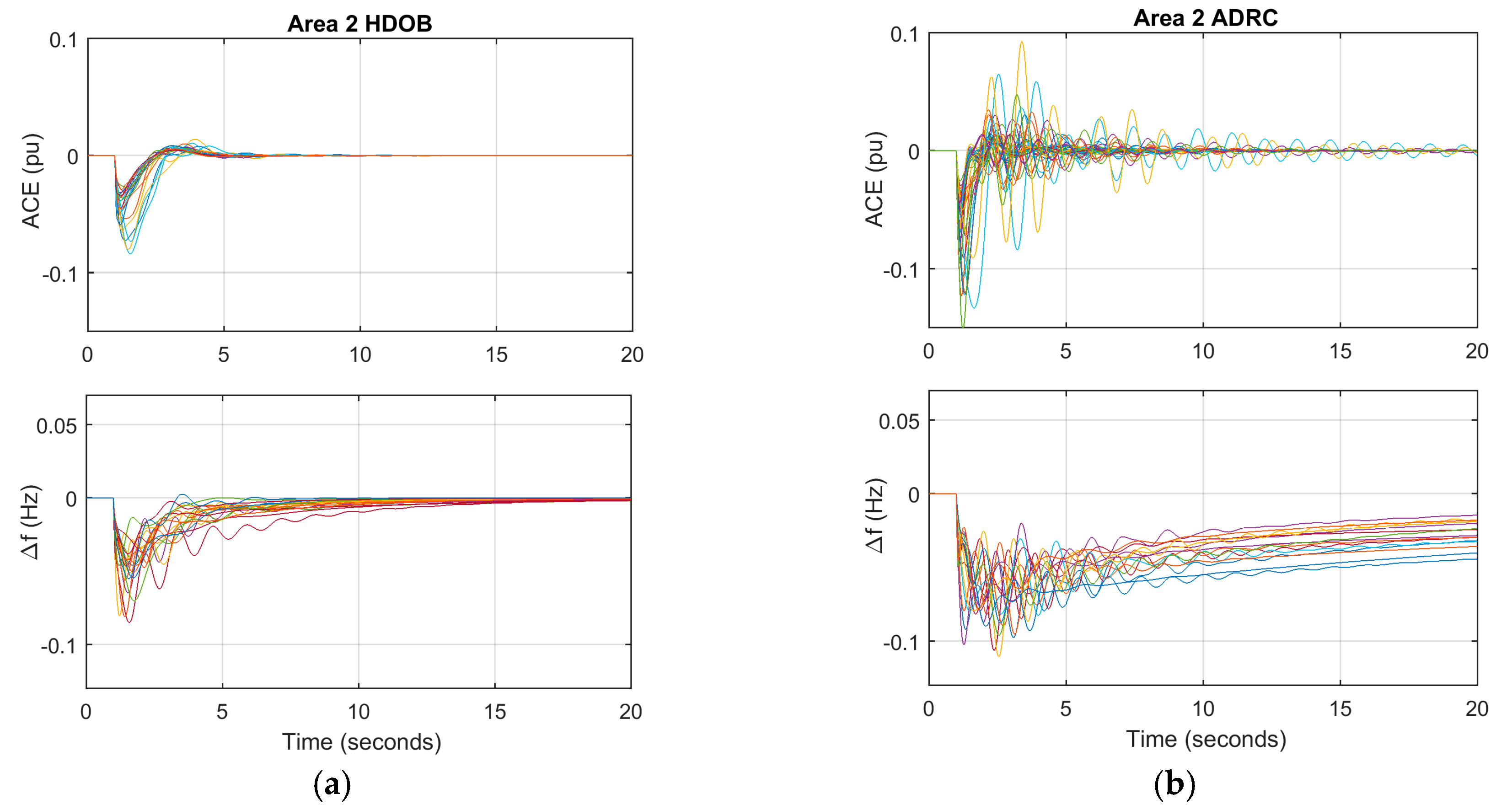
Figure 9.
Various response of LFC due to uncertain and in Area 3 with: (a) HDOB; (b) ADRC; after applying large-magnitude step load changes.
Figure 9.
Various response of LFC due to uncertain and in Area 3 with: (a) HDOB; (b) ADRC; after applying large-magnitude step load changes.
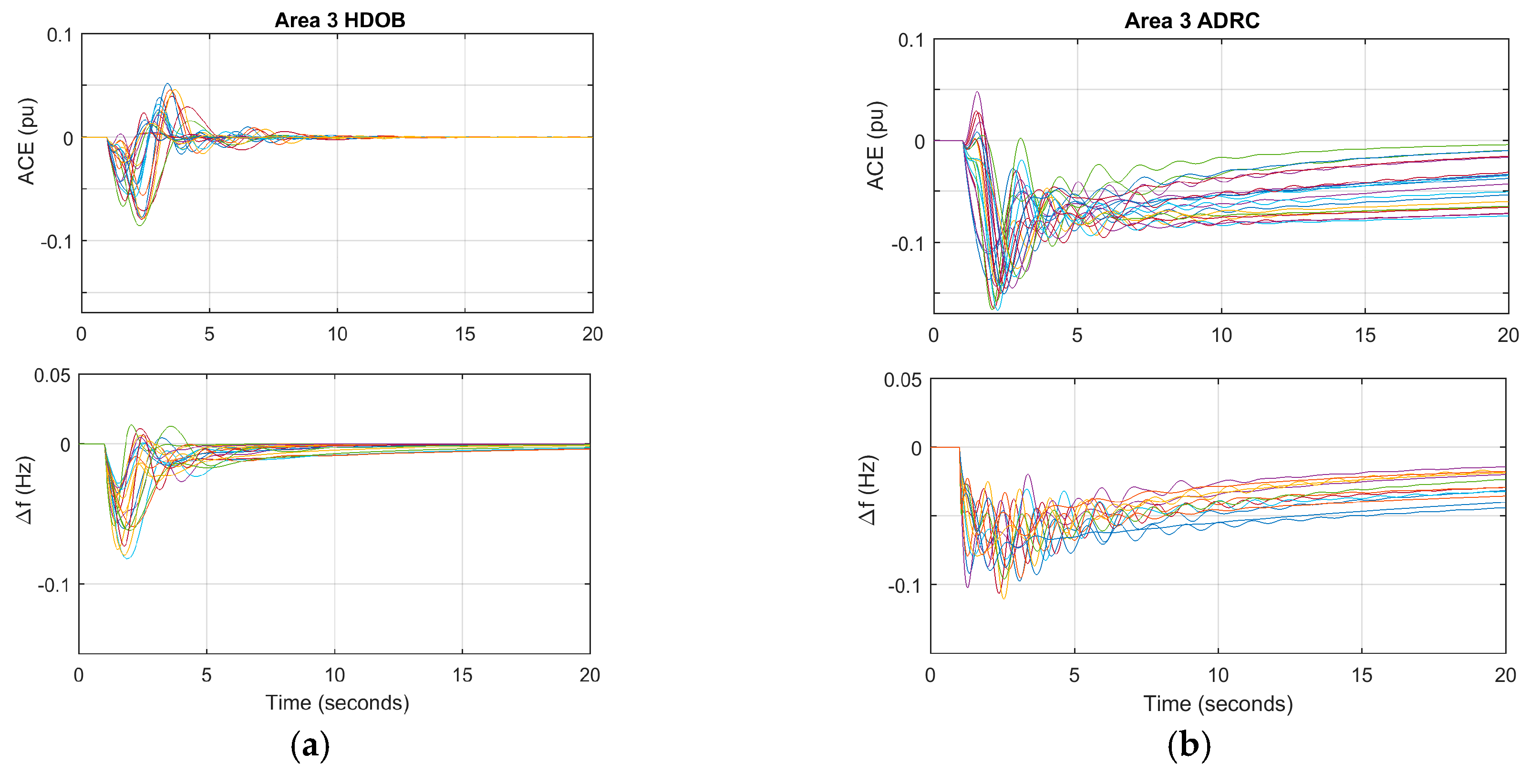
Figure 10.
Various response of LFC due to uncertain and in Area 4 with: (a) HDOB; (b) ADRC; after applying large-magnitude step load changes.
Figure 10.
Various response of LFC due to uncertain and in Area 4 with: (a) HDOB; (b) ADRC; after applying large-magnitude step load changes.
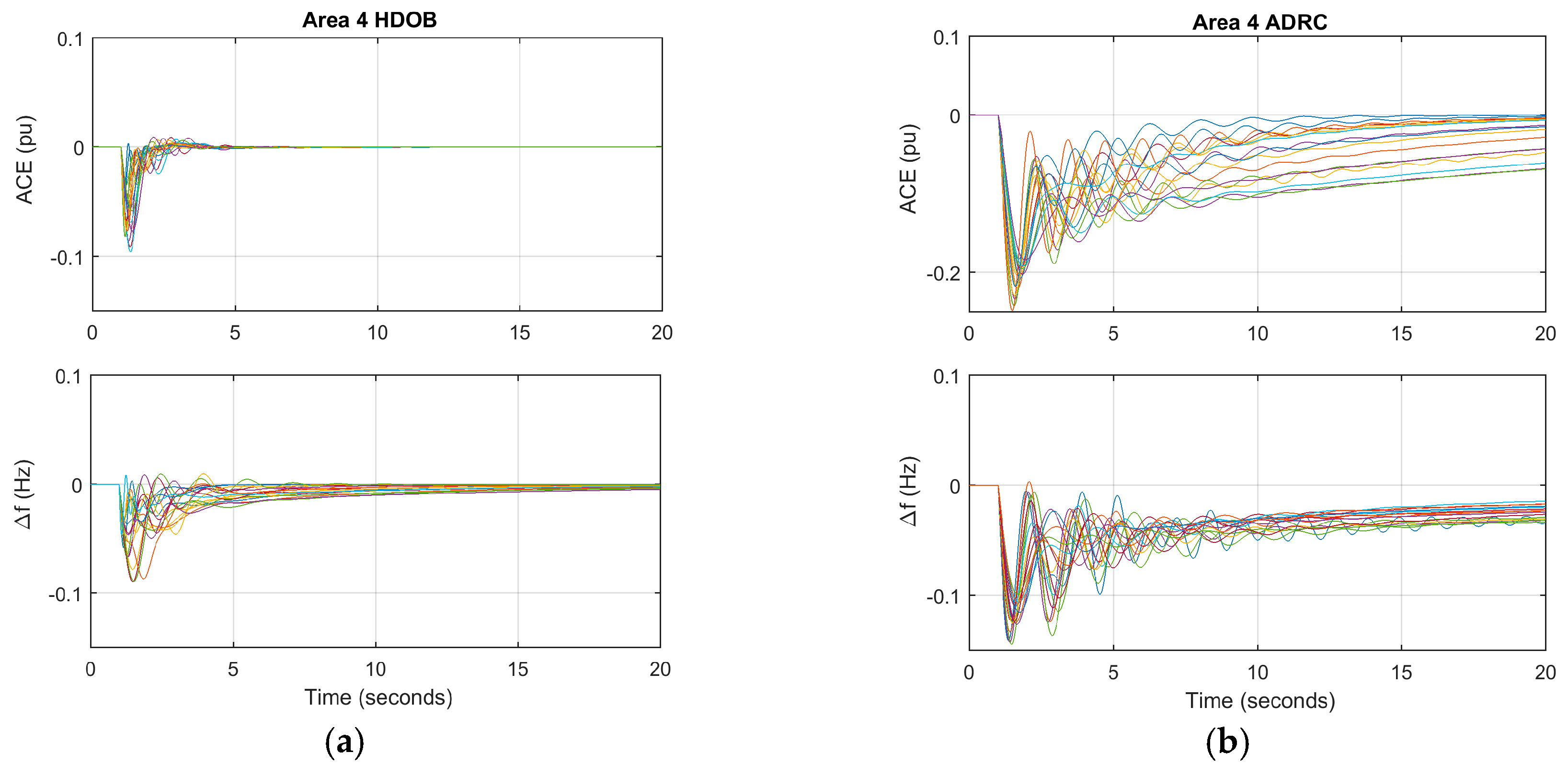
Figure 11.
Various response of LFC due to uncertain and in Area 5 with: (a) HDOB; (b) ADRC; after applying large-magnitude step load changes.
Figure 11.
Various response of LFC due to uncertain and in Area 5 with: (a) HDOB; (b) ADRC; after applying large-magnitude step load changes.

Figure 12.
Oscillating disturbance employed to the system.

Figure 13.
ACE and of the HDOB and ADRC based LFC with oscillating load changes and uncertain and in: (a) Area 1; (b) Area 2; (c) Area 3; (d) Area 4; and (e) Area 5.
Figure 13.
ACE and of the HDOB and ADRC based LFC with oscillating load changes and uncertain and in: (a) Area 1; (b) Area 2; (c) Area 3; (d) Area 4; and (e) Area 5.
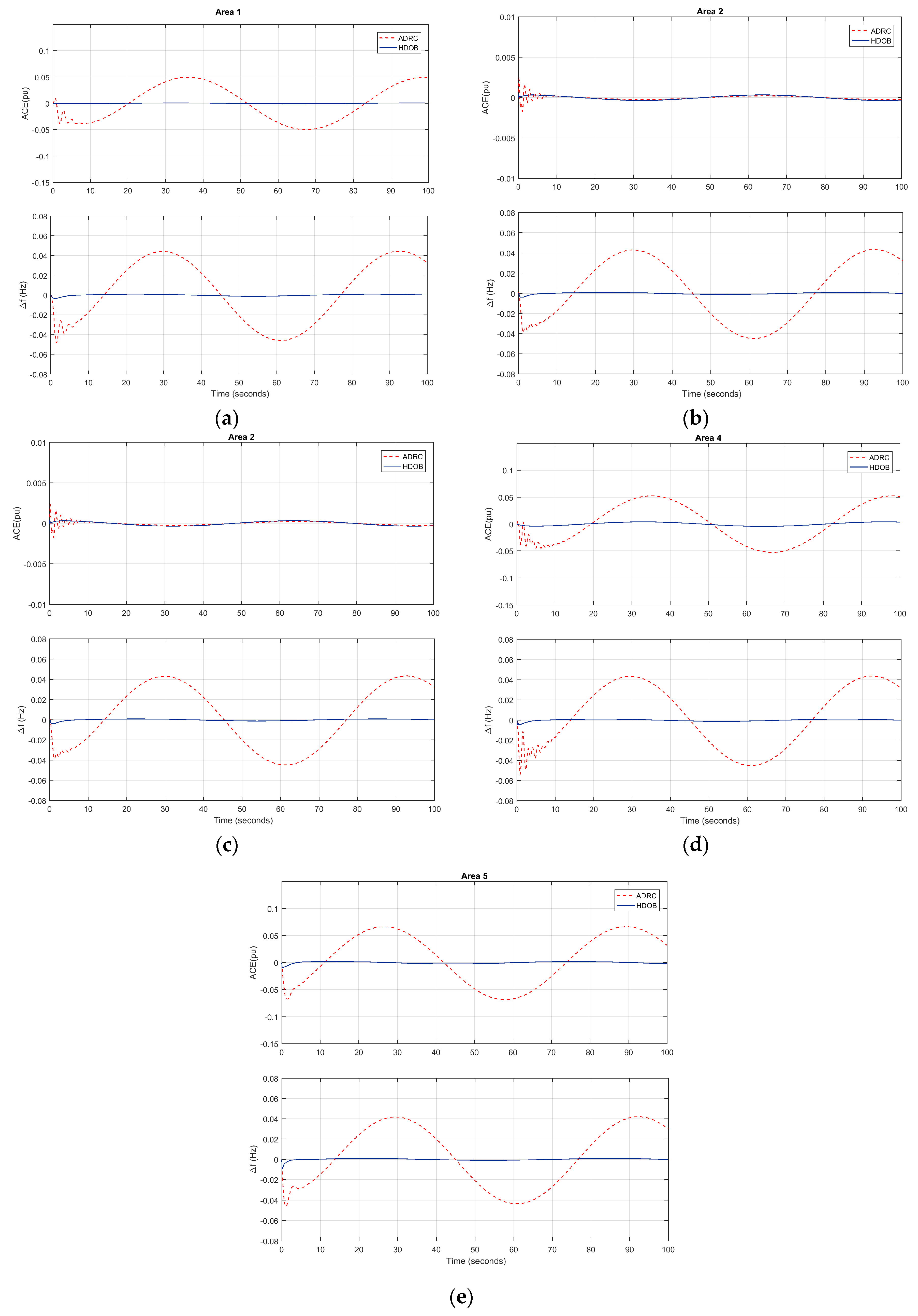
Figure 14.
ACE of the HDOB based LFC with random load changes and considering measurement delay.
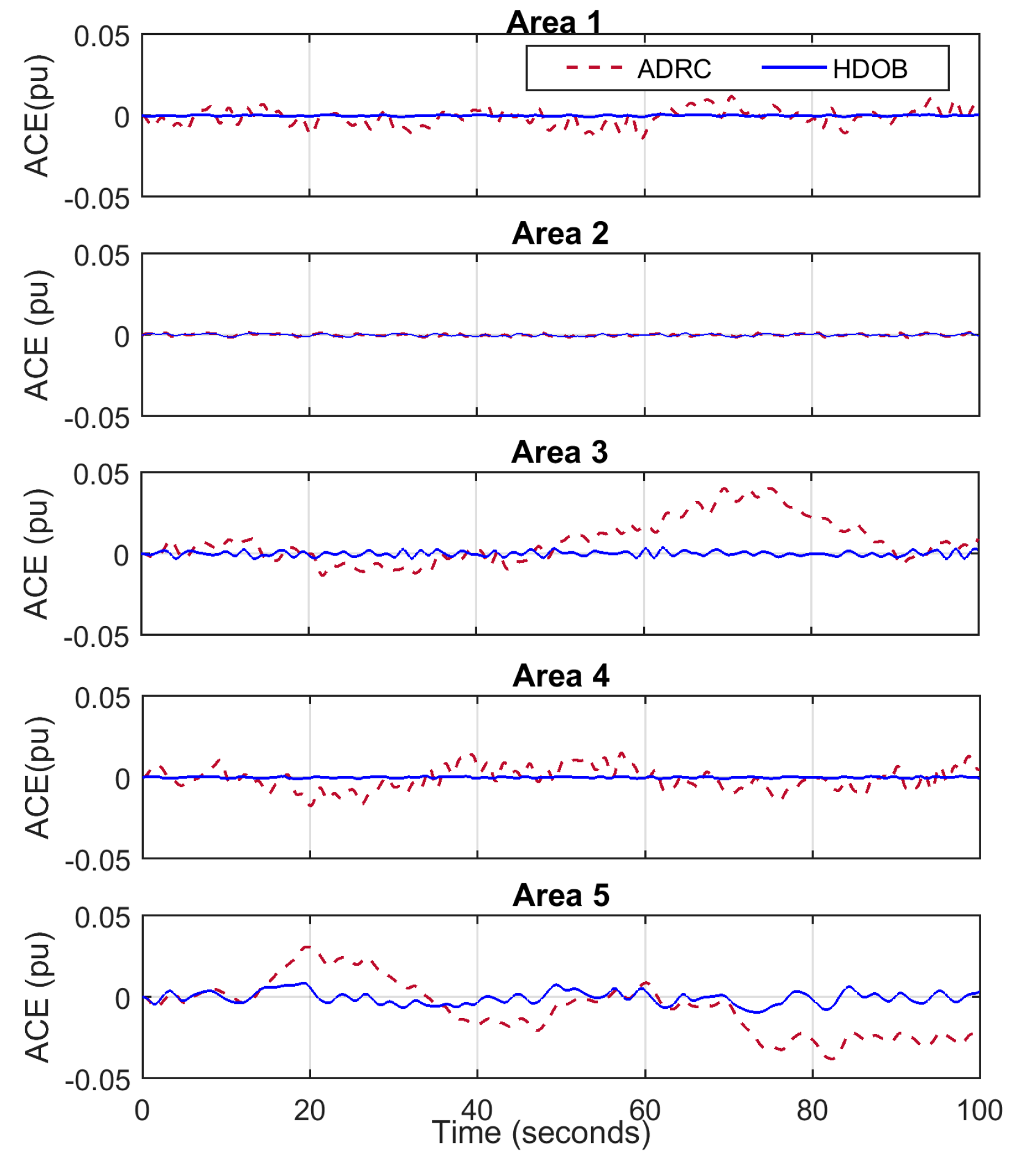
Figure 15.
ACE, frequency deviation , and control signal of the HDOB based LFC with large amplitude step load changes and considering measurement delays in: (a) Area 1; (b) Area 2; (c) Area 3; (d) Area 4; and (e) Area 5.
Figure 15.
ACE, frequency deviation , and control signal of the HDOB based LFC with large amplitude step load changes and considering measurement delays in: (a) Area 1; (b) Area 2; (c) Area 3; (d) Area 4; and (e) Area 5.


Figure 16.
The topology to study the robustness of controller against different number of connected generators in: (a) and ; (b) and ; and (c) and .
Figure 16.
The topology to study the robustness of controller against different number of connected generators in: (a) and ; (b) and ; and (c) and .

Figure 17.
Responses of LFC in Area 1 with different number of generators with: (a) HDOB; (b) ADRC; after applying large-magnitude step load changes.
Figure 17.
Responses of LFC in Area 1 with different number of generators with: (a) HDOB; (b) ADRC; after applying large-magnitude step load changes.

Figure 18.
Responses of LFC in Area 3 with different number of generators with: (a) HDOB; (b) ADRC; after applying large-magnitude step load changes.
Figure 18.
Responses of LFC in Area 3 with different number of generators with: (a) HDOB; (b) ADRC; after applying large-magnitude step load changes.

Figure 19.
The topology to study the robustness of controller against different number of connected areas in Area 2 and 3 corresponding with (a) two; (b) three; (c) four; (d) five; connected areas.
Figure 19.
The topology to study the robustness of controller against different number of connected areas in Area 2 and 3 corresponding with (a) two; (b) three; (c) four; (d) five; connected areas.
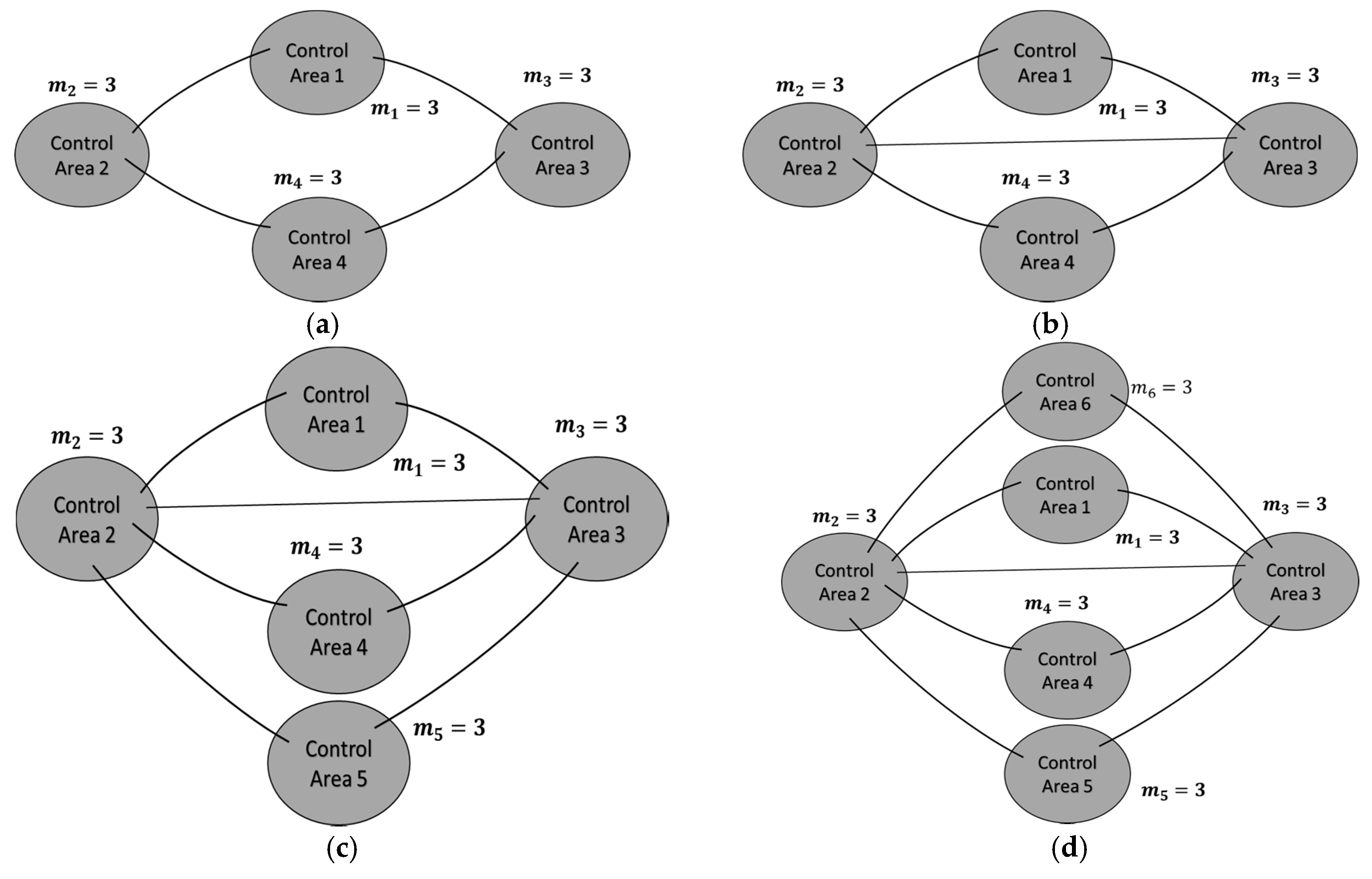
Figure 20.
Responses of LFC in: (a) Area 2; (b) Area 3 with different number of connected areas after applying large-magnitude step load changes.
Figure 20.
Responses of LFC in: (a) Area 2; (b) Area 3 with different number of connected areas after applying large-magnitude step load changes.

© 2017 by the authors. Licensee MDPI, Basel, Switzerland. This article is an open access article distributed under the terms and conditions of the Creative Commons Attribution (CC BY) license (http://creativecommons.org/licenses/by/4.0/).
Share and Cite
MDPI and ACS Style
Rosyiana Fitri, I.; Kim, J.-S.; Song, H. High-Gain Disturbance Observer-Based Robust Load Frequency Control of Power Systems with Multiple Areas. Energies 2017, 10, 595. https://doi.org/10.3390/en10050595
AMA Style
Rosyiana Fitri I, Kim J-S, Song H. High-Gain Disturbance Observer-Based Robust Load Frequency Control of Power Systems with Multiple Areas. Energies. 2017; 10(5):595. https://doi.org/10.3390/en10050595
Chicago/Turabian StyleRosyiana Fitri, Ismi, Jung-Su Kim, and Hwachang Song. 2017. "High-Gain Disturbance Observer-Based Robust Load Frequency Control of Power Systems with Multiple Areas" Energies 10, no. 5: 595. https://doi.org/10.3390/en10050595
Note that from the first issue of 2016, this journal uses article numbers instead of page numbers. See further details here.