
Optimal Allocation of Energy Storage System Considering Multi-Correlated Wind Farms


1
College of Automation, Harbin Engineering University, Harbin 150001, China
2
Department of Electrical Engineering and Computer Science, University of Wisconsin-Milwaukee, Milwaukee, WI 53211, USA
3
Department of Electrical Engineering, Chung Yuan Christian University, Chung Li District, Taoyuan City 32023, Taiwan
*
Author to whom correspondence should be addressed.
Energies 2017, 10(5), 625; https://doi.org/10.3390/en10050625
Submission received: 19 January 2017
/
Revised: 13 April 2017
/
Accepted: 27 April 2017
/
Published: 4 May 2017
(This article belongs to the Special Issue Sustainable and Renewable Energy Systems)
Abstract
:With the increasing penetration of wind power, not only the uncertainties but also the correlation among the wind farms should be considered in the power system analysis. In this paper, Clayton-Copula method is developed to model the multiple correlated wind distribution and a new point estimation method (PEM) is proposed to discretize the multi-correlated wind distribution. Furthermore, combining the proposed modeling and discretizing method with Hybrid Multi-Objective Particle Swarm Optimization (HMOPSO), a comprehensive algorithm is explored to minimize the power system cost and the emissions by searching the best placements and sizes of energy storage system (ESS) considering wind power uncertainties in multi-correlated wind farms. In addition, the variations of load are also taken into account. The IEEE 57-bus system is adopted to perform case studies using the proposed approach. The results clearly demonstrate the effectiveness of the proposed algorithm in determining the optimal storage allocations considering multi-correlated wind farms.
1. Introduction
Due to the ever-increasing concern over the global climate change and fossil energy decrease, interest in wind power has drawn more attention. However, a high penetration of wind power raises a problem of system instability, caused by the nature of wind uncertainty. The goal of economic emission dispatch (EED) with the energy storage system is to minimize the power system cost and emissions meanwhile ensuring the stability and power quality with facilitating penetration of distributed wind resources.
In recent years, many researchers have focused on solving the EED problem associated with wind power [1,2,3,4,5,6,7]. Kumar and Suna in [1] developed a chemical reaction optimization algorithm based on the chemical molecular reaction to optimize total cost in wind–fossil-fuel-based power systems. With the help of this method, both environmental emissions and transmission losses are reduced. Zhan et al. [2] presented a multi-objective evolutionary algorithm to solve combined economic and emission dispatch problem incorporating the wind power, which decreased both the cost and the emission. In order to reduce the emissions, Denny and O’Malley [3] developed a forecasting method for wind power, which is utilized in the dispatch decisions. In [5], Tan et al. utilized two-point estimation method combined with particle swarm optimization to solve the stochastic economic load dispatch problem in microgrid which integrates the renewable energy generation. A traditional low-carbon emission dispatch analysis combined with the impact of wind power was proposed in [7].
However, the integration of a significant amount of wind power into power systems causes crucial challenges with determining optimal emission reduction, which result from its uncertainties. Especially, many wind sites are geographically close; therefore, interdependency of wind speeds at different sites should be considered in EED [8,9,10,11,12]. As mentioned in [13], various approaches such as Monte Carlo simulation and analytical solutions have been employed to model the correlation of the multiple dependent wind sources. Monte Carlo simulation technology is introduced in [14] to calculate the indices of load expectation and the loss of energy expectation considering the wind speed correlation between the wind farms. In [15], Vallée et al. used the method of Monte Carlo simulation to consider the impact of uncertain system parameters on optimal power flow, but any Monte Carlo method requires intensive simulations to reach convergence. In order to reduce the computational burden, the analytical probabilistic methods were proposed as follows. The authors in [16] made use of the first-order second-moment method (FOSMM) to account for the uncertainties and correlations of the system load. The cumulant method (CM) in [17] was developed to study probability load flow. Due to the simplification used in FOSMM and CM, these two methods may result in relatively large errors. PEM can overcome the above demerits of analytical methods, which utilizes deterministic routines in solving the probabilistic problems while requiring low computational simulations [18]. In [19], an efficient point estimate method was proposed to take uncertainty of nodal data and line parameters into account in the load-flow computations and to estimate the corresponding variations in the solution.
In this paper, the wind speed correlation between the two wind farms and their joint distribution is modeled by the Clayton-Copula method combined with a new PEM to discretize the joint distribution. The main advantages of the proposed method are twofold: (1) high computational efficiency when modeling and discretizing the joint distribution and (2) easy scale-up when dealing with multiple (more than two) wind farms. Furthermore, combining the proposed modeling and discretizing method with Hybrid Multi-Objective Particle Swarm Optimization (HMOPSO) [20,21,22], this paper develops an optimum energy storage allocation method considering inter-dependent wind farms to minimize wind-penetrated power system operation cost and emission. In addition, the load variation is considered by peak and off-peak load levels.
2. Problem Formulation
The goal of this study is to analyze the economic allocation of ESSs by considering the joint distribution of multi-correlated wind farms. The EED problem with ESSs incorporating multi-correlated wind farms is formulated by the reduction of COx emissions along with system cost minimization. The objective function encompasses the joint probability, power system operation cost and greenhouse gas emissions.
2.1. Modeling Multiple Dependent Wind Probability
Clayton-Copula method is used in this paper to model the joint probability of multi-correlated wind sources. Clayton-Copula method is a subset of the Copula method family which transfers multivariate marginal distributions of random variables into one-dimensional marginal [23,24,25]. Among various types of copulas, the Clayton-Copula is mostly used to study correlated risks because of their ability to capture dependence and the easiness of the construction and the implementation [26]. Unlike Normal-Copula and t-Copula, Clayton-Copula can be employed to joint marginal distributions together, which follows the different types of the distribution [27].
Let denote the joint cumulative distribution function with marginal and . Then there exists Clayton-Copula such that for all x and y:
where a is the correlation coefficient. Then the bivariate probability density function can be obtained by Equation (2):
With the help of the Clayton-Copula function, the marginal distribution of random variables for wind power and their dependency structure are constructed.
2.2. Discretizing Joint Distribution
Instead of using Monte Carlo method, a novel PEM is proposed in this paper to discretize the continuous multi-correlated wind power distribution. The basic concept of this discretizing method can be separated into two parts:
- (1)
- Calculate the first few moments of wind joint distribution when one of the wind farms is at its limits either zero or full wind power;
- (2)
- Find the remaining correlated finite points representing both wind farms generating power not at their limits. The procedure of the discretization are described as follows.
2.2.1. The Boundary Points
- (1)
- (2)
- Calculate the joint probabilities () when the output power of wind farm 1 is 0 MW combining with L different discretized wind powers in wind farm 2. L points in boundary are obtained.
- (3)
- Calculate the probabilities () when the output power in wind farm 2 is 0 MW combining with K different discretized wind powers in wind farm 1. K points in boundary can be obtained.
- (4)
- Calculate the probabilities () when the wind power in wind farm 1 achieves maximum combining with L different discretized wind power in wind farm 2. L boundary points are attained.
- (5)
- Calculate the probabilities () when the wind power in wind farm 2 achieves maximum combining with K different discretized wind power in wind farm 1. K boundary points are attained.
Note that the total number of discretized wind power in the boundary is 2K + 2L − 4 because 4 points are duplicating points.
2.2.2. The Interior Points
The remaining correlated discrete points (interior points) are calculated by integrating Clayton-Copula method with a PEM, which is given in below:
where and are the rated wind power of wind farm 1 and wind farm 2, respectively; , , represents the mean, the standard deviation, and the central moment of ; is the probability of interior points; denotes the total probability of interior points, which is equal to one minus the total probability of boundary points; denotes the standardized value of .
Consequently, altogether (K − 2) × (L − 2) interior points are finally determined. It was noticed that these interiors points are calculated not based on the discrete points obtained in the boundary point calculation and the total sum of all probabilities is equal to one, which is as shown in Equation (7):
2.3. Objective Function
The goal of this paper is optimally allocating the ESSs and generator outputs in order to reduce the total expected system operation cost and emissions, while considering the uncertainties and correlations of multiple wind farms and the variations of loads. The multi-objective functions are given by (8):
where is the total number of points of the discretized wind power; and denote the probability of peak-load condition and off peak-load condition; is the probability of i-th discrete point for the joint distribution of two wind farms; is the total operation cost at the i-th or k-th discrete point ($/h) with the peak load or off peak load; is the total emission at the i-th or k-th discrete point (kg/h) with the peak load or with the off peak load:
where NG is the number of generators; is the fuel cost of generator j ($/h); is the COx emission of generator j (kg/h); is the cost of ESS ($/h); , , are the fuel cost coefficients of generator j; , , represent the COx emission coefficients of generator j; is the operation and maintenance cost of ESS, which is taken to be $29/MWh [30] in this paper; denotes the power capacity of installed ESS (MW).
The first objective function in (8) is to calculate the total expected operation cost by optimally allocating ESS and determining the outputs of all the different types of generators factoring in the wind distribution as well as considering peak and off-peak loads. Due to the environmental concern, the emission equation in the second objective function of (8) is proposed to decrease the gaseous pollutants.
2.4. Problem Constraints
There are two types of constraints considered in this research: equality and inequality constraints.
2.4.1. Equality Constraints
These constraints (11) are related to the nonlinear power flow equations:
2.4.2. Inequality Constraints
The inequality constraints contain the bus voltages, the reactive power of generation and the tap of the transformer. The inequality constraints are shown as follows:
where is the RMS value of the bus i voltage; represents the reactive power of generator i, and denotes the tap of transformer i.
3. Solution Method
In order to solve the EED problem considering multiple dependent wind farms, the copula method combined with the proposed PEM is implemented to calculate the discretized joint probability of two inter-dependent wind farms, one in Madison and the other in Milwaukee. The algorithm of HMOPSO is applied to minimize the operation cost and emission and the algorithm consists of MOPSO with NSGA-II [31] for solving the multi-objective problems, and the probability power flow for obtaining the system status considering the probabilistic wind distribution. Additionally, the MOPSO with NSGA-II is detailed in the part of Appendix B.
3.1. Discretizing Multi-Correlated Wind Distribution
3.1.1. Wind Distribution
A 10-year daily wind speed data for the cities of Madison and Milwaukee in USA is used to fit the Weibull distribution, which is shown in Equation (13):
where is called the shape parameter, and is the scale parameter.
To obtain the wind power distribution, a linear approximation equation is utilized as follows:
where W is the injected power. X is actual wind speed. M is the maximum power of wind turbine. and are the linear coefficients. , and , respectively, denote the cut-in wind speed, cut-out wind speed and normal wind speed.
The rated power for the cities of Madison and Milwaukee are 45 MW and 330 MW, respectively derived from 30% penetration. The cut-in, cut-out, and rated speed are 3.5 m/s, 40 m/s, and 13.5 m/s, respectively. The parameters are summarized in Table 1.
Since Madison and Milwaukee are relatively close in geographical and metrological terms, the wind distributions of the two sites cannot be assumed to be independent so it is necessary to consider the wind speed dependencies. In this paper, a bivariate distribution between these two wind farms is constructed by Clayton-Copula method described in Section 2. By applying the Weibull distribution (Equation (13)) into Clayton-Copula method (Equation (2)), the bivariate probability density function can be rewritten as shown in Equation (15):
where is the sum of the probabilities of the interior points.
3.1.2. Discretizing Wind Power Joint Distribution
Following the procedure given in Section 2, the joint distribution can be discretized as follows.
- (1)
- The boundary points
- Calculate the probabilities (, ) when the output power of wind farm 1 is 0 MW or reaches the maximum combining with five different discretized wind powers of wind farm 2. Consequently, 10 discrete points are obtained;
- Apply the same algorithm into wind farm 2 and the probabilities that are and are determined. 10 discrete points are obtained herein.
- (2)
- The interior points
- The interior discrete probability points of the joint distribution are decided by Equations (3)–(6) and (13). Three points are selected for each wind farm distribution in the calculation and a total of 9 discrete probability points are obtained.
The total discrete probability points including both boundary and interior points are 25. The sum of the 25 discrete probabilities is equal to one. Table 2 shows the results of the 25 discrete probabilities and their corresponding wind power contribution from each. More specifically, the first 16 points are boundary points, and the others are interior points.
3.1.3. Combination Method for High-Dimensional Correlated Wind Distribution
The Clayton-Copula method can be used to build multivariate distribution of dimensions more than two. The proposed PEM can also discretize the joint distribution of higher dimension easily. Supposing that there are three dependent wind farms and their joint probability can be calculated by Equation (16):
Then the joint probability density function can be obtained:
The joint probability of correlated wind power can be redefined as:
Similarly, the new continuous distribution can be discretized using the new PEM.
3.2. Hybrid MOPSO for Economic Emission Dispatch
By incorporating a fast and elitist multi-objective algorithm and probabilistic load flow calculation, a HMOPSO algorithm is developed to search for the best combination of the placements and sizes of energy storage devices in power systems. A mixed-integer MOPSO [32,33,34] is applied to optimally locate and rate the storage. As a part of the probabilistic load flow, Newton–Raphson power flow calculates the power equations for the constraints.
The procedure of HMOPSO to solve the EED problem associated with multi-correlated wind farms can be summarized as follows:
- (1)
- Randomly generate population P with N particles for initializing all generators’ voltage, output power and position and size of ESS. The random selections of swarm of particles considering constraints and corresponding velocity for each particle are initialized.
- (2)
- Model joint probability of multi-wind farms by Clayton-Copula method.
- (3)
- Discretize the joint wind power distribution into 25-point distribution by the new proposed estimation method, which has been discussed in Section 3, 25 scenarios in two different load conditions for each study case are created.
- (4)
- Through probabilistic power flow, evaluate the particles by fitness function and recall their best positions associated with the best fitness value.
- (5)
- Check and preserve the and , if the algorithm has not yet converged, update the and .
- (6)
- Duplicate population P to population Q to form a combined population R and update the position and velocity of each particle.
- (7)
- Sort the members in population R through NSGA-II with elitism algorithm for selecting N best solutions to renew population P.
- (8)
- Repeat Steps 4–7 until all the scenarios are considered.
4. Result and Discussion
4.1. System Configuration
The proposed HMOPSO algorithm has been applied to IEEE 57-bus system and compared with several other methods in order to test its quality and robustness. The system consists of 7 generations and 42 loads, where bus 1 is the slack bus, buses 3, 6, 9, 12 are defined as power-voltage (PV) nodes, and other buses are real and reactive power (PQ) nodes [35]. According to the sensitivity analysis, wind generations are added to bus 2 and bus 8 with the rated size of 45 MW and 330 MW, respectively.
A typical daily load profile for a community in the city of Madison is scaled. The peak-load condition, which is 1250.80 MW, and the off peak-load condition, which is 750.48 MW (60% of maximum load) are selected as variable load conditions to conduct HMOPSO algorithm in case studies.
4.2. Economic and Emission Analysis
The impacts of the integration of wind power, two different load conditions, and ESSs in five cases are studied and compared to demonstrate the effectiveness of the proposed method.
Case 1: A regular probabilistic load flow analysis for the system considering the entire joint wind power distribution, but without ESS installation;
Case 2: An optimal load flow analysis to determine the best ESS allocation under the worst-case scenario assuming zero wind power for both wind farms;
Case 3: HMOPSO with ESS considering the entire joint wind distribution;
Case 4: Multi-objective genetic algorithm (MOGA) with ESS considering the entire joint wind distribution;
Case 5: HMOPSO with ESS without considering the joint wind distribution;
Case 6: HMOPSO with ESSs considering three dependent wind farms.
The resultant costs and emissions of Cases 1–3 are listed in Table 3.
Case 1
It can be seen from Table 3 that the total operation cost and emissions are reduced with the increase of wind power in Case 1. The operation cost in peak load condition varies from $108,816/h to $56,937/h according to the changes of total wind power from 0 to 375 MW and the emissions decrease from 86,162 kg/h to 29,556 kg/h. Similarly, the operation cost in off peak-load condition has the same pattern, which ranges from $23,660/h to $35,280/h with the emission from 24,289 kg/h to 6027.7 kg/h. However, since no ESS was considered in this case, the system confronts with both low voltage and high power loss problems. Specifically, when the total wind power is 0, the voltage at the wind generator buses and load area experiences a low voltage problem associated with a high power loss, which is 128.85 MW. Under this situation, even if the outputs of the diesel generators reach the maximum, the low voltages still appear at buses 20, 30, 31, 32, 33 and 34, which drop to 0.96 p.u. below.
Case 2
In this case, the optimal load flow analysis is implemented to determine the locations and the corresponding sizes of ESSs under the worst operating condition, considering the zero wind power situation. In this case, buses 14, 45, 47 and 52 are found to be the best places to install ESSs with sizes of 29.98 MW, 26.30 MW, 12.66 MW and 15.14 MW, separately. The system is then operated with the given allocation of ESSs, considering twenty-five different wind power situations in peak-load and off peak-load conditions; even though the total operation cost and emissions are significantly reduced comparing with Case 1, no matter the total size of the installed ESSs or the cost and emissions are higher than that in Case 3.
In addition, the total expected operation cost in Case 2 is equal to $44,309.38/h and the expected emission is calculated to 23,454.15 kg/h by Equation (8) and the fuel cost and emission coefficients are given in Table 4.
Case 3
In this case, the optimal ESS allocation considers the entire joint wind distribution. The proposed HMOPSO is implemented to minimize the operation cost and emissions through searching the optimal ESS allocation and generator outputs. In HMOPSO, the algorithm starts with randomly generating a swarm of particles and each particle initializes a random ESS size within constraints at each bus. The size of ESSs is evaluated by the cost and emissions function and will be updated by HMOPSO. In the end, the size of ESSs at some buses becomes zero, which means that these buses do not need to install any ESS. The remaining ESSs converge to their optimal allocations. As a result, the best placements for ESSs in Case 3 are buses 10, 32, 46 and 52 with the size of 12.89 MW, 13.12 MW, 16.50 MW and 29.87 MW, respectively. Table 5 describes optimization results for expected values of operation cost, greenhouse gas emissions and power loss in four cases. Similar to Case 2, the total operation cost and emissions are reduced, and voltage profiles are improved.
The results from Table 5 show that the proposed method in Case 3, which considered the entire wind distribution and employed the HMOPSO, delivered the best results in all categories. Notice that the total expected operation cost is calculated to be $38,522.24/h in Case 3, which is much less than that in Case 2, indicating that the allocation of ESSs selected by the proposed HMOPSO algorithm is much better than only using the worst-case scenario. Supposing that the system operated in one year (8760 h), the system in Case 3 will save $506,953, 46.4/year compared to the conventional optimization result, which is determined by the worst case. Furthermore, even though the total size of ESS in Case 3 is less than that in Case 2, the COx emissions decreased more, which is 17.59% lower than that in Case 2.
Case 4
In order to demonstrate the effectiveness of HMOPSO, the method of MOGA is compared to solve EED problem in the same operation situation as Case 3. As shown in Table 5, the total operation cost and emissions are $40,754.70/h and 20,939.28 kg, respectively, which are both higher than that in Case 3. Furthermore, the total size of ESSs found by MOGA is larger than HMOPSO, which is 80.78 MW. However, the system has to confront with a higher voltage deviation than that in Case 3 and the voltage deviation is calculated by , which is shown in Figure 1. In addition, the computing speed of the HMOPSO is faster. Specifically, the time to operate the algorithm in Case 4 once is 224.52 s which is 12.35 s slower than that in Case 3.
Case 5
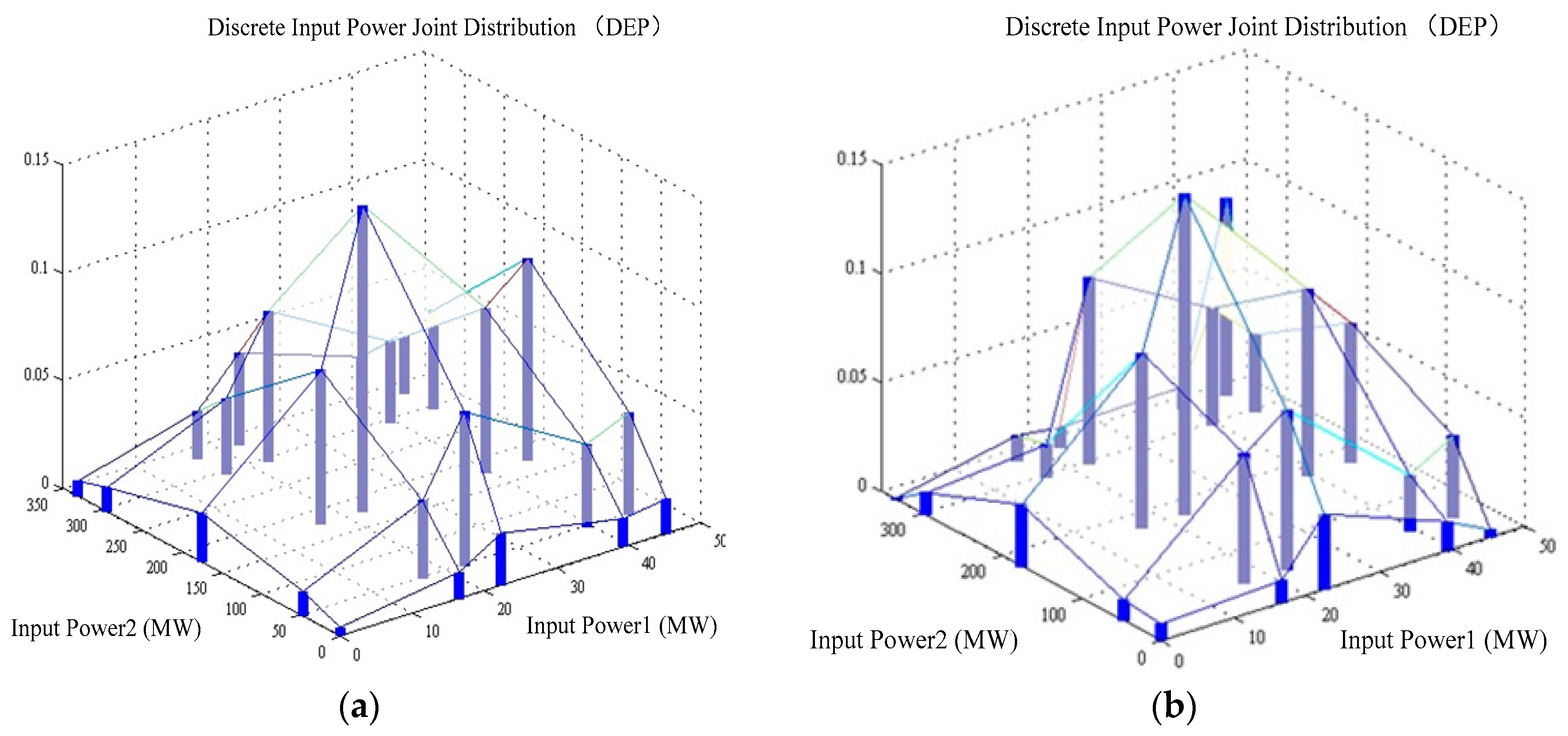
In this case, the two wind distributions are assumed to be independent. The probability comparison between with and without joint wind distribution is shown in Figure 2. By utilizing the HMOPSO in the same way, the best allocation for ESSs without considering joint wind distribution are found to be 10, 32, 46 and 52 with the size of 26.37 MW, 17.01 MW, 9.35 MW and 25.86 MW, respectively. The total expected operation cost is calculated to be $39,455.60/h by Equation (8), which is $933.36/h higher than that considering joint wind distribution in Case 3 and the total expected emission without joint wind distribution is 21,976.54 kg/h, which is 12.05% more than that with joint wind distribution. Furthermore, all values obtained in this case are larger than those in Case 3 for the sake of ignoring the interdependency of multi-correlated wind farms.
Case 6
With the rapid development of the renewable technology, three correlated wind farms are considered in this case. These wind farms are installed in buses 2, 3 and 8 with the rated power of 45 MW, 125 MW and 330 MW, respectively. By applying the HMOPSO in the same way, the best allocation for ESSs in Case 6 are found to be 10, 32, 46, 49 and 52 with the size of 24.88 MW, 23.64 MW, 26.10 MW, 7.76 MW and 28.49 MW, respectively. The total expected operation cost is optimized to be $62,008.81/h with 42,967 kg/h CO2 emissions. In addition, according to the hardware condition of Intel Core i5-4460, 3.20 GHz CPU and a 4.00 GB RAM, it takes 1053.86 s to operate the optimization algorithm once.
5. Conclusions
As the penetration of wind power continues to increase in the power grids, it becomes important to consider the uncertainties of multi-correlated wind power generations when optimizing the placements and sizes of ESSs. In this paper, the Clayton-Copula method incorporating with a new PEM is presented to calculate the discretized joint probability for two dependent wind farms. A HMOPSO algorithm is applied to solve economic emission problems associated with optimal energy storage allocation, where the variation of loads is also taken into account. Furthermore, unlike many other optimization methods which only consider the worst-case scenario or the expected wind power scenario, the entire multi-correlated wind power distribution is taken into account in the optimization. The approach of how to scale up to more interdependent wind farms is also discussed. An IEEE 57-bus system is adopted to perform case studies. The results illustrate the importance of considering the wind speed correlations between the wind farms and also show that the proposed approach is able to find optimal placements and sizes of ESSs for reduction of total cost and emissions. In the future study, both the annualized investment costs of the renewable energy and ESSs and the load profile along the year (8760 h) as well as the single cycle of the ESSs will be considered.
Acknowledgments
This study was financially supported by the Ministry of Industry and Information Technology in cooperation with the Ministry of Finance under grant GK110900004 and by Fundamental Research Funds for the Central Universities under HEUCFJ170403 as well as by China Postdoctoral Science Foundation.
Author Contributions
All authors contributed to this collaborative work. Shuli Wen performed the research and discussed the results; Hai Lan modeled the multi-correlated wind distribution and designed the optimal algorithm; Qiang Fu, David C. Yu, Ying-Yi Hong and Peng Cheng suggested the research idea and contributed to the writing and revision of the paper. All authors approved the manuscript.
Conflicts of Interest
The authors declare no conflict of interest.
Appendix A
List of Abbreviations and Symbols:
| HMOPSO | Hybrid multi-objective particle swarm optimization |
| EED | Economic emission dispatch |
| ESS | Energy storage system |
| FOSMM | First-order second-moment method |
| CM | Cumulant method |
| PEM | Point estimation methods |
| MOPSO | Multi-objective particle swarm optimization |
| NSGA-II | Nondominated Sorting Genetic Algorithms-II |
| MOGA | Multi-objective genetic algorithm |
| Joint cumulative distribution function | |
| Correlation coefficient | |
| Bivariate probability density function | |
| and | The rated wind power of wind farm 1 and wind farm 2 |
| The mean of (X, Y) | |
| The standard deviation of (X, Y) | |
| The central moment of (X, Y) | |
| The probability of interior points | |
| The total probability of interior points | |
| z | The standardized value of (X, Y) |
| The probability of peak-load condition | |
| The probability of off peak-load condition | |
| The probability of i-th discrete point for the joint distribution of two wind farm | |
| Total operation cost at the i-th or k-th discrete point ($/h) with the peak load or off peak load | |
| The total emission at the i-th or k-th discrete point (kg/h) with the peak load or with the off peak load | |
| The number of generators | |
| The fuel cost of generator j ($/h) | |
| ECOx (PGj) | The COx emission of generator j (kg/h) |
| Cw | The cost of wind power generator ($/h) |
| Cs | The cost of ESS ($/h) |
| aj, bj, cj | The fuel cost coefficients of generator j |
| θj, δj, γj | The COx emission coefficients of generator j |
| Copw | The operation cost of wind power generator ($/MWh) |
| Cops | The operation cost of ESS ($/MWh) |
| Pwind | The power of wind power generator (MW) |
| Pstorage | The capacity of installed ESS (MW) |
| k | Shape parameter of distribution |
| λ | Scale parameter of distribution |
| W | The injected power |
| X | Actual wind speed |
| M | The maximum power of wind turbine |
| N | The total number of points of the discretized wind power |
| α and β | The linear coefficients |
| Vci, Vco and Vno | The cut-in wind speed, cut-out wind speed and normal wind speed |
| p11-33 | The sum of the probabilities of the interior points |
| The expected voltage | |
| The maximum of voltage deviation |
Appendix B
Appendix B.1. MOPSO
Particle Swarm Optimization (PSO) is a heuristic optimization technique first developed in 1995 by Kennedy and Eberhart and the basic idea behind the PSO algorithm is that a population called a swarm is randomly created, consisting of individuals called particles. Each particle, representing a potential solution of the optimization problem, flies through an N-dimensional search space at a random velocity, and updates its position based on its own best exploration, best swarm global experience, and its previous velocity vector according to the following equations:
where is the inertia weight; and are acceleration constants; and denote two random numbers in the range of [0, 1]; is the best position i particle achieved based on its own experience, ; represents the best particle position based on overall swarm’s experience, .
To improve the efficiency and accuracy, a linearly decreasing inertia weight from maximum value to minimum is applied to update the inertia weight:
where and are the initial and final inertia weights, is the maximum iteration number.
Appendix B.2. NSGA-II
Different from the optimization problem with single-objective function, NSGA-II was developed to sort the best solutions for selecting the final answer. The details of NSGA-II are described as follows.
Firstly, the population P of size N cooperated with Q in the same size N to form a whole population R, whose size is 2N. Then the population R is sorted by nondomination with the elitism algorithm and each individual has its own front number. Now, the members belong to the best nondominated set , are of best solutions in the whole population, which range from the highest front number and dominate the other group. If the size of is less than N, the algorithm will continue to select new members, which come from subsequent front numbers until the size of new population gets to be equal to or larger than N. Lastly, crowed-comparison operator is used to choose N exact members if the size of is larger than N. The new population is used for the next iteration and, in every iteration, the individuals compete with each other by binary tournament selection operator.
References
- Kumar, R.P.; Suna, H. Economic emission dispatch for wind-fossil-fuel-based power system using chemical reaction optimisation. Int. Trans. Electr. Energy Syst. 2015, 25, 3248–3274. [Google Scholar]
- Zhan, J.P.; Wu, Q.H.; Guo, C.X.; Zhang, L.L.; Bazargan, M. Impacts of wind power penetration on combined economic and emission dispatch. In Proceedings of the 4th IEEE/PES Innovative Smart Grid Technologies Europe (ISGTEurope), Copenhagen, Denmark, 6–9 October 2013; pp. 1–5. [Google Scholar]
- Denny, E.; O’Malley, M. Wind generation, power system operation, and emissions reduction. IEEE Trans. Power Syst. 2006, 21, 341–347. [Google Scholar] [CrossRef]
- Madaeni, S.H.; Member, S.; Sioshansi, R.; Member, S. Using demand response to improve the emission Benefits of Wind. IEEE Trans. Power Syst. 2013, 28, 1385–1394. [Google Scholar] [CrossRef]
- Tan, Y.; Cao, Y.; Li, C.; Li, Y.; Yu, L.; Zhang, Z.; Tang, S. Microgrid stochastic economic load dispatch based on two-point estimate method and improved particle swarm optimization. Int. Trans. Electr. Energy Syst. 2015, 25, 2144–2164. [Google Scholar] [CrossRef]
- Li, Z.; Guo, Q.; Sun, H.; Wang, Y.; Xin, S. Emission-concerned wind-EV coordination on the transmission grid side with network constraints: Concept and case study. IEEE Trans. Smart Grid 2013, 4, 1692–1704. [Google Scholar] [CrossRef]
- Palanichamy, C.; Babu, N.S. Day-night weather-based economic power dispatch. IEEE Trans. Power Syst. 2002, 17, 469–475. [Google Scholar] [CrossRef]
- Arjmand, R.; Rahimiyan, M. Statistical analysis of a competitive day-ahead market coupled with correlated wind production and electric load. Appl. Energy 2016, 161, 153–167. [Google Scholar] [CrossRef]
- Díaz, G.; Casielles, P.G.; Coto, J. Simulation of spatially correlated wind power in small geographic areas—Sampling methods and evaluation. Int. J. Electr. Power Energy Syst. 2014, 63, 513–522. [Google Scholar] [CrossRef]
- Pope, K.; Naterer, G.F.; Dincer, I.; Tsang, E. Power correlation for vertical axis wind turbines with varying geometries. Int. J. Energy Res. 2011, 35, 423–435. [Google Scholar] [CrossRef]
- Correia, P.F.; Ferreira de Jesus, J.M. Simulation of correlated wind speed and power variates in wind parks. Electr. Power Syst. Res. 2010, 80, 592–598. [Google Scholar] [CrossRef]
- Lyu, J.K.; Heo, J.H.; Park, J.K.; Kang, Y.C. Probabilistic approach to optimizing active and reactive power flow in wind farms considering wake effects. Energies 2013, 6, 5717–5737. [Google Scholar] [CrossRef]
- Li, Y.; Li, W.; Yan, W.; Yu, J.; Zhao, X. Probabilistic optimal power flow considering correlations of wind speeds following different distributions. IEEE Trans. Power Syst. 2014, 29, 1847–1854. [Google Scholar] [CrossRef]
- Pudjianto, D.; Pudjianto, D.; Ramsay, C.; Ramsay, C.; Strbac, G.; Strbac, G. Virtual power plant and system integration of distributed energy resources. IET Renew. Power Gener. 2007, 1, 10–16. [Google Scholar] [CrossRef]
- Vallée, F.; Lobry, J.; Deblecker, O. Application and comparison of wind speed sampling methods for wind generation in reliability studies using non-sequential Monte Carlo simulations. Eur. Trans. Electr. Power 2009, 19, 1002–1015. [Google Scholar] [CrossRef]
- Li, X.; Li, Y.; Zhang, S. Analysis of probabilistic optimal power flow taking account of the variation of load power. IEEE Trans. Power Syst. 2008, 23, 992–999. [Google Scholar]
- Schellenberg, A.; Rosehart, W.; Aguado, J. Cumulant-based probabilistic optimal power flow (P-OPF) with Gaussian and Gamma distributions. IEEE Trans. Power Syst. 2005, 20, 773–781. [Google Scholar] [CrossRef]
- Hong, H.P. An efficient point estimate method for probabilistic analysis. Reliab. Eng. Syst. Saf. 1998, 59, 261–267. [Google Scholar] [CrossRef]
- Su, C. Probabilistic load-flow computation using point estimate method. IEEE Trans. Power Syst. 2005, 20, 1843–1851. [Google Scholar] [CrossRef]
- Moghaddam, A.A.; Seifi, A.; Niknam, T. Multi-operation management of a typical micro-grids using Particle Swarm Optimization: A comparative study. Renew. Sustain. Energy Rev. 2012, 16, 1268–1281. [Google Scholar] [CrossRef]
- Deb, K.; Pratap, A.; Agarwal, S.; Meyarivan, T. A fast and elitist multiobjective genetic algorithm: NSGA-II. IEEE Trans. Evol. Comput. 2002, 6, 182–197. [Google Scholar] [CrossRef]
- Meng, M. A hybrid particle swarm optimization algorithm for satisficing data envelopment analysis under fuzzy chance constraints. Expert Syst. Appl. 2014, 41, 2074–2082. [Google Scholar] [CrossRef]
- Segers, J. Hybrid copula estimators. J. Stat. Plan. Inference 2015, 160, 23–34. [Google Scholar] [CrossRef]
- Koirala, K.H.; Mishra, A.K.; D’Antoni, J.M.; Mehlhorn, J.E. Energy prices and agricultural commodity prices: Testing correlation using copulas method. Energy 2015, 81, 430–436. [Google Scholar] [CrossRef]
- Artem’eva, S.M.; Burmann, H.-W. On the relationship between modular and hypergeometric functions. Differ. Equ. 2009, 45, 151–158. [Google Scholar] [CrossRef]
- Al-Harthy, M.; Begg, S.; Bratvold, R.B. Copulas: A new technique to model dependence in petroleum decision making. J. Pet. Sci. Eng. 2007, 57, 195–208. [Google Scholar] [CrossRef]
- Nelsen, R.B. An Introduction to Copulas, 2nd ed.; Springer: New York, NY, USA, 2006. [Google Scholar]
- Fu, Q.; Yu, D.; Ghorai, J. Probabilistic load flow analysis for power systems with multi-correlated wind sources. In Proceedings of the 2011 IEEE Power & Energy Society General Meeting, Detroit, MI, USA, 24–28 July 2011. [Google Scholar]
- Wen, S.; Lan, H.; Fu, Q.; Yu, D.C.; Zhang, L. Economic allocation for energy storage system considering wind power distribution. IEEE Trans. Power Syst. 2015, 30, 644–652. [Google Scholar] [CrossRef]
- Eyer, J.; Corey, G. Energy Storage for the Electricity Grid: Benefits and Market. Potential Assessment Guide; Sandia National Laboratories: Albuquerque, NM, USA, 2010.
- Buayai, K.; Ongsakul, W.; Mithulananthan, N. Multiobjective micro-grid planning by NSGA-II in primary distribution system. Eur. Trans. Electr. Power 2012, 22, 170–187. [Google Scholar] [CrossRef]
- Kennedy, J.; Eberhart, R. Particle swarm optimization. In Proceedings of the IEEE International Conference on Neural Networks, Perth, Australia, 27 November–1 December 1995; Volume IV, pp. 1942–1948. [Google Scholar]
- Eberhart, R.; Kennedy, J. A new optimizer using particle swarm theory. In the Proceedings of the Sixth International Symposium on Micro Machine and Human Science (MHS’95), Nagoya, Japan, 4–6 October 1995; pp. 39–43. [Google Scholar]
- Hu, X.; Shi, Y.; Eberhart, R. Recent advances in particle swarm. In Proceedings of the 2004 Congress on Evolutionary Computation (CEC2004), Portland, OR, USA, 19–23 June 2004; Volume I, pp. 90–97. [Google Scholar]
- Bus Power Flow Test Case. Available online: http://www.ee.washington.edu/research/pstca/pf57/pg_tca57bus.htm (accessed on 3 May 2017).
Figure 1.
The expected voltage deviation for different cases.
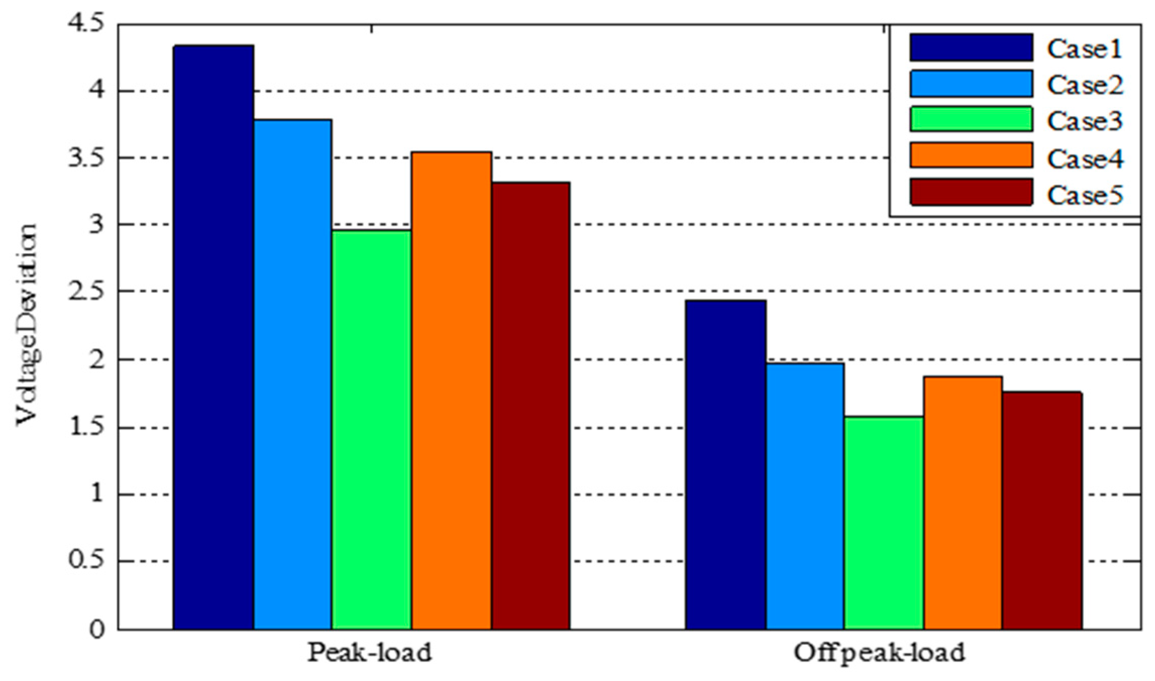
Figure 2.
The probability comparison between independent and dependent wind distributions. (a) Independent probability; and (b) dependent probability.
Figure 2.
The probability comparison between independent and dependent wind distributions. (a) Independent probability; and (b) dependent probability.

Table 1.
Parameters of two farms.
| Wind Farm | k | λ | α | β | Max Power |
|---|---|---|---|---|---|
| 1 | 2.5034 | 10.0434 | −15.75 | 4.5 | 45 MW |
| 2 | 2.4 | 11.5 | −115.5 | 33 | 330 MW |
Table 2.
Probability of multi-correlated wind farms.
| Point | Probability (%) | Wind Farm 1 (MW) | Wind Farm 2 (MW) |
|---|---|---|---|
| 1 | 0.759 | 0 | 0 |
| 2 | 1.015 | 0 | 46.57 |
| 3 | 3.457 | 0 | 173.96 |
| 4 | 1.330 | 0 | 293.18 |
| 5 | 0.334 | 0 | 330 |
| 6 | 0.072 | 45 | 0 |
| 7 | 1.199 | 45 | 46.57 |
| 8 | 0.932 | 45 | 173.96 |
| 9 | 1.037 | 45 | 293.18 |
| 10 | 9.043 | 45 | 330 |
| 11 | 0.934 | 16.46 | 0 |
| 12 | 2.815 | 22.23 | 0 |
| 13 | 1.014 | 39.09 | 0 |
| 14 | 3.710 | 16.46 | 330 |
| 15 | 6.402 | 22.23 | 330 |
| 16 | 3.518 | 39.09 | 330 |
| 17 | 5.897 | 15.96 | 47.51 |
| 18 | 7.320 | 15.96 | 175.28 |
| 19 | 2.546 | 15.96 | 294.23 |
| 20 | 8.019 | 21.47 | 47.51 |
| 21 | 14.690 | 21.47 | 175.28 |
| 22 | 8.574 | 21.47 | 294.23 |
| 23 | 1.496 | 38.24 | 47.51 |
| 24 | 8.574 | 38.24 | 175.28 |
| 25 | 5.350 | 38.24 | 294.23 |
Table 3.
Operation cost and emissions in different load conditions.
| No. | Peak Load Condition | Off Peak-Load Condition | ||||||||||
|---|---|---|---|---|---|---|---|---|---|---|---|---|
| Case 1 | Case 2 | Case 3 | Case 1 | Case 2 | Case 3 | |||||||
| Cost 104 $/h | Em 104 kg/h | Cost 104 $/h | Em 104 kg/h | Cost 104 $/h | Em 104 kg/h | Cost 104 $/h | Em 104 kg/h | Cost 104 $/h | Em 104 kg/h | Cost 104 $/h | Em 104 kg/h | |
| 1 | 10.88 | 8.62 | 10.13 | 7.70 | 7.35 | 5.34 | 3.53 | 2.43 | 3.09 | 1.81 | 2.69 | 1.62 |
| 2 | 9.92 | 7.62 | 8.82 | 6.44 | 7.25 | 5.09 | 3.2 | 2.03 | 3.13 | 1.78 | 2.4 | 1.28 |
| 3 | 7.8 | 5.36 | 5.93 | 3.70 | 5.7 | 3.52 | 2.61 | 1.22 | 2.33 | 1.09 | 2.28 | 0.84 |
| 4 | 8.37 | 3.77 | 5.44 | 2.79 | 4.68 | 2.40 | 2.38 | 0.77 | 2.29 | 0.66 | 2.27 | 0.50 |
| 5 | 7.02 | 3.36 | 5.11 | 2.39 | 4.55 | 2.13 | 2.36 | 0.69 | 2.35 | 0.46 | 2.32 | 0.39 |
| 6 | 10.65 | 8.35 | 8.43 | 6.22 | 6.84 | 4.97 | 3.44 | 2.30 | 3.36 | 2.03 | 2.49 | 1.63 |
| 7 | 9.7 | 7.37 | 7.75 | 5.49 | 6.36 | 4.29 | 3.12 | 1.92 | 2.89 | 1.51 | 2.38 | 1.29 |
| 8 | 7.63 | 5.16 | 6.49 | 3.97 | 5.38 | 3.28 | 2.56 | 1.15 | 2.51 | 0.90 | 2.35 | 0.85 |
| 9 | 6.24 | 3.61 | 5.32 | 2.66 | 4.53 | 2.32 | 2.37 | 0.73 | 2.31 | 0.47 | 2.28 | 0.47 |
| 10 | 5.9 | 3.21 | 5.23 | 2.53 | 4.63 | 2.12 | 2.36 | 0.65 | 2.29 | 0.42 | 2.28 | 0.42 |
| 11 | 10.56 | 8.26 | 10.48 | 7.97 | 7.48 | 5.54 | 3.4 | 2.26 | 2.47 | 1.56 | 2.43 | 1.50 |
| 12 | 9.63 | 7.28 | 8.4 | 5.96 | 7.32 | 5.06 | 3.1 | 1.88 | 2.62 | 1.43 | 2.53 | 1.32 |
| 13 | 7.57 | 5.09 | 6.48 | 3.85 | 5.15 | 3.03 | 2.55 | 1.13 | 2.43 | 0.84 | 2.3 | 0.78 |
| 14 | 6.19 | 3.55 | 5.26 | 2.62 | 4.6 | 2.16 | 2.37 | 0.71 | 2.28 | 0.52 | 2.27 | 0.44 |
| 15 | 5.86 | 3.16 | 5.25 | 2.41 | 4.54 | 2.05 | 2.36 | 0.64 | 2.3 | 0.37 | 2.29 | 0.30 |
| 16 | 10.33 | 7.99 | 7.87 | 5.68 | 7.84 | 5.68 | 3.31 | 2.14 | 3.13 | 1.78 | 2.41 | 1.44 |
| 17 | 9.41 | 7.04 | 8.63 | 6.12 | 6.48 | 4.35 | 3.02 | 1.78 | 2.5 | 1.21 | 2.35 | 1.19 |
| 18 | 7.39 | 4.89 | 6.49 | 3.95 | 5.32 | 3.15 | 2.51 | 1.06 | 2.32 | 0.98 | 2.31 | 0.80 |
| 19 | 6.06 | 3.39 | 5.55 | 2.76 | 4.73 | 2.09 | 2.36 | 0.68 | 2.35 | 0.58 | 2.24 | 0.44 |
| 20 | 5.74 | 3.01 | 4.91 | 2.13 | 4.49 | 2.03 | 2.37 | 0.61 | 2.31 | 0.32 | 2.3 | 0.29 |
| 21 | 10.25 | 7.90 | 9.83 | 7.28 | 6.71 | 4.78 | 3.28 | 2.10 | 3.18 | 1.87 | 2.43 | 1.52 |
| 22 | 9.33 | 6.95 | 9.06 | 6.47 | 6.07 | 4.04 | 3 | 1.74 | 2.88 | 1.39 | 2.47 | 1.15 |
| 23 | 7.34 | 4.82 | 5.88 | 3.46 | 5.34 | 3.05 | 2.5 | 1.03 | 2.43 | 0.76 | 2.3 | 0.69 |
| 24 | 6.01 | 3.33 | 5.11 | 2.37 | 4.44 | 2.09 | 2.36 | 0.67 | 2.31 | 0.43 | 2.3 | 0.41 |
| 25 | 5.7 | 2.96 | 4.99 | 2.21 | 4.37 | 1.98 | 2.37 | 0.60 | 2.33 | 0.47 | 2.31 | 0.42 |
Table 4.
Cost and emission coefficients of generators.
| Generator | a | b | c | θ (10−2) | δ (10−2) | γ (10−2) |
|---|---|---|---|---|---|---|
| 1 | 0 | 20 | 0.0775795 | 3.965 | −5.876 | 7.632 |
| 3 | 0 | 20 | 0.25 | 2.543 | −6.047 | 5.638 |
| 6 | 0 | 40 | 0.01 | 4.258 | −5.094 | 4.586 |
| 9 | 0 | 40 | 0.01 | 4.258 | −5.094 | 4.586 |
| 12 | 0 | 20 | 0.0322581 | 4.872 | −4.663 | 5.449 |
Table 5.
Expected value in four cases.
| Cost, Emissions and Loss | Case 1 | Case 2 | Case 3 | Case 4 | |
|---|---|---|---|---|---|
| Peak load | Cost ($/h) | 74,169.85 | 64,138.60 | 53,709.76 | 57,871.49 |
| Emission (kg/h) | 48,861.97 | 38,261.51 | 31,038.75 | 33,525.19 | |
| Power loss (MW) | 67.3 | 53.94 | 35.35 | 40.87 | |
| Off peak-load | Cost ($/h) | 26,137.06 | 24,480.15 | 23,334.71 | 23,637.90 |
| Emission (kg/h) | 11,280.01 | 8646.78 | 7617.79 | 8353.37 | |
| Power loss (MW) | 15.01 | 12.19 | 9.18 | 10.23 | |
| Total operation cost ($/h) | 50,153.46 | 44,309.38 | 38,522.24 | 40,754.70 | |
| Total operation emission (kg/h) | 30,070.99 | 23,454.15 | 19,328.27 | 20,939.28 | |
| Total size of ESS (MW) | 0 | 84.08 | 72.38 | 80.78 | |
© 2017 by the authors. Licensee MDPI, Basel, Switzerland. This article is an open access article distributed under the terms and conditions of the Creative Commons Attribution (CC BY) license (http://creativecommons.org/licenses/by/4.0/).
Share and Cite
MDPI and ACS Style
Wen, S.; Lan, H.; Fu, Q.; Yu, D.C.; Hong, Y.-Y.; Cheng, P. Optimal Allocation of Energy Storage System Considering Multi-Correlated Wind Farms. Energies 2017, 10, 625. https://doi.org/10.3390/en10050625
AMA Style
Wen S, Lan H, Fu Q, Yu DC, Hong Y-Y, Cheng P. Optimal Allocation of Energy Storage System Considering Multi-Correlated Wind Farms. Energies. 2017; 10(5):625. https://doi.org/10.3390/en10050625
Chicago/Turabian StyleWen, Shuli, Hai Lan, Qiang Fu, David C. Yu, Ying-Yi Hong, and Peng Cheng. 2017. "Optimal Allocation of Energy Storage System Considering Multi-Correlated Wind Farms" Energies 10, no. 5: 625. https://doi.org/10.3390/en10050625
Note that from the first issue of 2016, this journal uses article numbers instead of page numbers. See further details here.