A Game Theoretical Approach Based Bidding Strategy Optimization for Power Producers in Power Markets with Renewable Electricity

Abstract

In a competitive electricity market with substantial involvement of renewable electricity, maximizing profits by optimizing bidding strategies is crucial to different power producers including conventional power plants and renewable ones. This paper proposes a game-theoretic bidding optimization method based on bi-level programming, where power producers are at the upper level and utility companies are at the lower level. The competition among the multiple power producers is formulated as a non-cooperative game in which bidding curves are their strategies, while uniform clearing pricing is considered for utility companies represented by an independent system operator. Consequently, based on the formulated game model, the bidding strategies for power producers are optimized for the day-ahead market and the intraday market with considering the properties of renewable energy; and the clearing pricing for the utility companies, with respect to the power quantity from different power producers, is optimized simultaneously. Furthermore, a distributed algorithm is provided to search the solution of the generalized Nash equilibrium. Finally, simulation results were performed and discussed to verify the feasibility and effectiveness of the proposed non-cooperative game-based bi-level optimization approach.

1. Introduction

Following the attempts in the USA, Britain, Australia and Russia, many countries have embarked on a massive reform of the electricity power market in recent decades [1]. As the document “The notice about the reform pilot of transmission and distribution price carried out in Shenzhen” was issued two years ago, electric power industry in China has undergone significant changes from the regulated monopoly to a deregulated electricity market. Several new kinds of market participants have emerged in this new market structure, for example utility companies that invested and established by social capitals, power exchange (PX) and independent system operator (ISO) [2].

Deregulated electricity markets are established for the purposes of improving system efficiency and optimizing resource allocation [3]. Meanwhile, it is important to strengthen the sustainability of the electric power industry. Renewable energy resources especially wind are being substantially developed and utilized to take the place of fossil fuels to tackle the severe impacts of global warming in many electric systems worldwide. Various countries have different policies for wind power generation; some of them take full acquisition, and some allow wind farms to take bids in the market. Due to the gradually mature wind power technology, government subsidies are less and less relatively, and wind power producers prefer to participate in electricity markets to maximize their profits [4]. However, the uncertainty of wind power generation is a major obstacle for wind power producers to take part in the electricity market. Accurate prediction of generation is hard to obtain even though forecasting techniques have considerably improved over the last few decades.

In a competitive electricity market, all power producers desire to make a healthy profit by adjust bidding strategies, and much research has been undertaken. For conventional or fossil fuel power producers, game theory and the bi-level optimization method [5,6] were used to simulate and optimize the bidding strategies of power producers. Zhang et al. [6] established a general multi-leader-one-follower nonlinear bi-level (MLNB) model to optimize strategic bidding, for which the upper level optimization problem is a noncooperative game problem. Moreover, related definitions of the MLNB based on the generalized Nash equilibrium were also provided. The noncooperative multi-leader-follower game is computationally intractable due to the nonconvexity in each player’s problem [7]. A class of remedial models was proposed to formulate the multi-leader-follower game as generalized Nash games with convex strategy sets in [7]. For renewable power producers, various methods have used stochastic models to generate optimal bidding strategies for wind power producers participating in liberalized electricity market with considering the uncertain output [3,8,9]. Pinson et al. [10] formulated a general methodology for deriving optimal bidding strategies based on probabilistic forecasts of wind production. For solving the randomness of renewable energy output, energy storage technologies [11,12], such as pumped-hydro storage and compressed air, are studied by several researchers. However, the availability of utility-scale storage is still limited. Imbalance cost is utilized to tackle the effect of uncertainty and intermittent output in [13,14]. Dai et al. [14] proposed a bilateral reserve market to cover the uncertainty and intermittency of wind power, where the bilateral reserve is provided by conventional power producers and consumed by wind power producers. However, they did not consider the impact of power producers’ bidding on real-time price and day-ahead price, which are obtained through forecasting and scenario generation in [14].

In view of large-scale new energy power penetration in the electricity market, several researches [15,16,17,18,19] consider new energy power producers as strategic players, which can optimize profit by participating in competitive bidding. Zugno et al. [15] and Baringo et al. [16] only consider wind power producers as strategic players either in the day-ahead market or in the real-time market. Dai et al. [17] proposed a bi-level stochastic optimization approach to maximize the profit of wind power producers, which submit a bidding strategy as strategic players in both the day-ahead market and real-time market. In [17], bidding strategies of other strategic conventional power producers have no effect on wind power producers. Actually, bidding strategies of conventional power producers and wind power producers will influence each other, and all of them can influence the market clearing price. In [18,19], conventional power producers and wind power producers as the same strategic players bid in the market, and the equilibrium problem with equilibrium constraints is formulated to maximize the total expected profit of all power producers. However, cooperation among power producers is difficult to achieve in practice, due to the selfish and profit-driven nature of power producers.

Different from the existing literature, this paper employs a non-cooperative game based on the bi-level optimization approach for multiple power producers to maximize profits by optimizing bidding strategies in a competitive electricity market considering the uncertainty and intermittency of renewable energy power. The main contributions of this paper include the following: (1) a non-cooperative game approach-based bi-level optimization is proposed to deal with a scenario in a competitive electricity market having multiple power producers, multiple utility companies, a PX and an ISO, where the payoff of the non-cooperative game is the profit of each power producer; (2) a distributed algorithm is presented to realize the optimization in terms of maximizing the profit of all power producers; (3) simulation results are discussed to verify the feasibility and efficiency of the proposed optimization method.

The rest of the paper is organized as follows. Section 2 presents the market framework that this paper studied; the cost model and the bid model for different types of power plants are presented. In Section 3, the profit model is described considering the premium mechanism. The novel proposed method of this paper for optimizing the bidding strategy based on the game-theoretic method is presented in Section 4. Simulation results are presented and discussed in Section 5. Finally, conclusions are provided in Section 6.

2. Problem Formulation

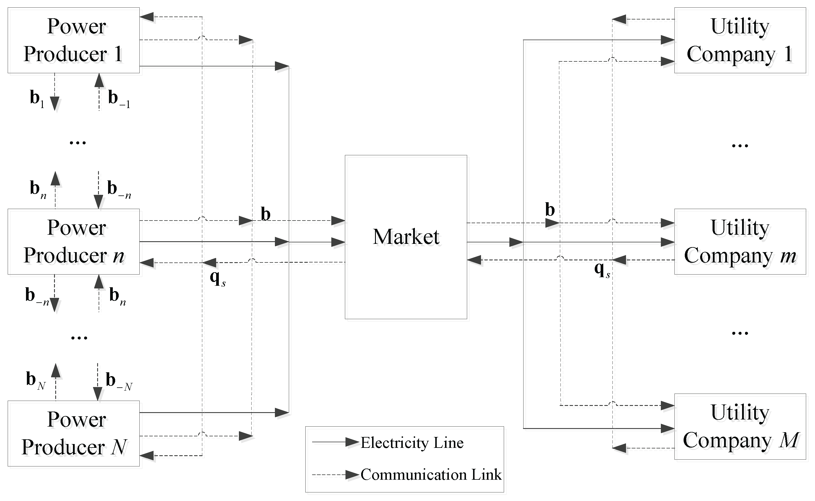
2.1. Market Framework

An electricity market is mainly formed by the medium and long-term trade market and spot market. In order to promote the development of renewable energy sources, only the spot market is studied in this paper considering the variability of renewable energy sources. The electricity market in various countries or regions has different characteristics, which can be suitable for the practical application scenarios. For example, the Pennsylvania-New Jersey-Maryland (PJM) electricity market in the United States includes the spot market, the capacity market, the ancillary services market and the financial transmission right market, where the spot market consists of day-ahead market and real-time market. Nord Pool operates a day-ahead market, an intraday market and a real-time market, which was established in 1993 and consisted of Norway, Sweden, Finland and Denmark [20,21].

Assume that there is one PX operating in the day-ahead market, the intraday market and the real-time balancing market, and one ISO checks the system safety to guarantee that electricity markets are operated under conditions of absolute security and stabilization. As shown in Figure 1, a pool-based electricity market is considered in which M utility companies submit load curves into the day-ahead market for trading time slot $h\in \mathcal{H}=\left\{1,\cdots ,H\right\}$ in the next operating day. One can choose each trading time slot as 15 min, and then, $H=$ 96. Let $\mathcal{M}=\left\{1,\cdots ,M\right\}$ and $\mathcal{N}=\left\{1,\cdots ,N\right\}$, where $\mathcal{M}$ and $\mathcal{N}$ denote the set of the utility company and the power producer, respectively. ISO provides superposition of M utility companies’ load curves to power producers. Then, N power producers, including conventional thermal power producers, wind power producers and solar power producers, can submit energy offer curves into day-ahead and intraday markets. In the day-ahead market, power producers need to propose bidding curves, including the maximum generating volume in the next operating day, before gate closure, which generally occurs at 12 a.m. in the current operating day [9]. In order to sell as much generating volume as possible, the predicted generating volume in the next operating day is taken as the maximum generating volume in bidding curves. Later, according to the rules of the PX, the ISO announces the market clearing price and cleared generating volume of each power producer, which is determined by using a single market clearing process. Due to the uncertainty and intermittency of wind and solar power, prediction error exists on the day-ahead market, which forecasts too far in advance. Power producers are allowed to resubmit bidding strategies on the intraday market, for which gate closure generally occurs between 30 min and 2 h before the time of actual power delivery. The intraday market deals with the deviation between the practical generating volume and that scheduled on the day-ahead market. Then, clearing results for power producers in the intraday market are determined by the ISO. The prediction errors on the intraday market are undertaken by the ISO, which ensures the real-time balance between offers and demands by buying or selling electricity in a real-time balancing market [21].

For the following modeling and analyzing, several assumptions are made as follows [10,14]: (1) predicted power generation on the intraday market can be considered to be practical generating volume; (2) power outputs of the thermal power producers can be precisely controlled, and errors of the thermal power producers are not considered; (3) the load prediction error is not considered; (4) all power producers have no market power in both day-ahead and intraday markets, namely bidding strategies of any power producers cannot have a significant impact on the market clearing price.

2.2. Cost Model

The generation cost of thermal power plants has been studied by many scholars, and it is widely accepted that generation cost is the quadratic function of generating volume [6]:

$$C_{th0}\left(q_{th}\right)=a_{th}{q}_{th}^2+b_{th}{q}_{th}+c_{th}$$

(1)

where $C_{th0}$ and $q_{th}$ denote generation cost and generating volume of thermal power plants and $a_{th}$, $b_{th}$, $c_{th}$ are fixed positive parameters of thermal power plants. Thermal power plants generate electricity by consuming fossil fuels, which produce a great deal of $\mathrm{C}{\mathrm{O}}_2$ and other atmospheric pollutants. For the purpose of environment protection and realization of sustainable development of the electric power industry, carbon emission factors can be included in the total generation cost under the deregulated environment of electricity market. Then,

$$C_{th}\left(q_{th}\right)=a_{th}{q}_{th}^2+b_{th}{q}_{th}+c_{th}+p_{ct}\mu q_{th}-p_{cr}\mu \left(1-\sigma \right)q_{th}$$

(2)

where $C_{th}$ is the total generation cost of thermal power plants, $p_{ct}$ and $p_{cr}$ are the carbon emission price at the transmitting end and receiving end, $\mu$ is unit electric energy carbon emission conversion factor of thermal power plants and $\sigma$ is the line loss rate.

The generation cost of wind farms mainly includes capital cost, maintenance and operation cost. Wind power is a renewable green energy, which requires no fuel cost, and it is the reason that wind power has been developed vigorously in the last few years. For wind farms, the capital cost is high while the operation cost is very low compared to thermal power plants. Generation cost can be divided into two parts: the fixed cost and the variable cost, which includes capital cost, maintenance and operation cost, respectively. Compared with the zero variable cost of the wind power plant in [19], this paper assumes that the variable cost has a linear relationship with generating volume [22]; thus,

$$C_{w0}\left(q_w\right)=b_w{q}_w+c_w$$

(3)

where $C_{w0}$ and $q_w$ are the generation cost and generating volume of wind farms and $b_w$, $c_w$ are fixed positive parameters of wind farms. Total generation cost of wind farms considering the carbon emission factors $C_w$ can be calculated as:

$$C_w\left(q_w\right)=b_w{q}_w+c_w-p_{cr}\mu \left(1-\sigma \right)q_w$$

(4)

Solar power also is a clean renewable energy, and solar power plants do not need the fuel cost to produce electricity. Similarly, compared to conventional thermal power plants, the capital cost of solar power plants is high, and the operation cost is very low. Therefore, the total generation cost of solar power plants considering the carbon emission factors $C_s$ can be expressed in the same way as wind farms:

$$C_s\left(q_s\right)=b_s{q}_s+c_s-p_{cr}\mu \left(1-\sigma \right)q_s$$

(5)

where $b_s$, $c_s$ are fixed positive parameters of solar power plants and $q_s$ is the generating volume of solar power plants.

2.3. Bidding Model

The marginal cost of thermal power plant $C_{thm}$ is calculated by:

$$C_{thm}\left(q_{th}\right)=2a_{th}{q}_{th}+b_{th}+p_{ct}\mu -p_{cr}\mu \left(1-\sigma \right)$$

(6)

which is a linear function of its generating volume $q_{th}$. Generally, power producers bid based on marginal cost to maximize their profit in a competitive electricity market. The bidding curve of thermal power plants can be described as a linear function, namely,

$$p_{thb}=a_{thb}{q}_{th}+b_{thb}$$

(7)

where $p_{thb}$ is the bid price of thermal power plants and $a_{thb}>0$, $b_{thb}$ are bidding parameters of thermal power plants.

When generating volume is increased, the variable cost of wind farms increases slightly due to the low operation cost. Fixed cost is always considered a constant, and the value is large [22], for which allocation to per unit generating volume will obviously decrease when generating volume is increased. Therefore, average generation cost will reduce when wind farms produce more generating volume. This means that wind power producers are willing to bid a lower price if they can obtain more power generation. Assume that the bidding curve of wind farms is a monotonically decreasing and linear function and can be described as [23,24,25]:

$$p_{wb}=a_{wb}{q}_w+b_{wb}$$

(8)

where $p_{wb}$ denotes the bid price of wind farms and $a_{wb}<0$, $b_{wb}$ are bidding parameters of wind farms.

Owing to the same characteristic as wind farms whose variable cost is low and fixed cost is comparatively high, solar power producers prefer to submit the bidding curve similar to wind power producers. Consequently, the bid price of solar power plants $p_{sb}$ is given by,

$$p_{sb}=a_{sb}{q}_s+b_{sb}$$

(9)

where $a_{sb}<0$, $b_{sb}$ are the bidding parameters of solar power plants.

3. Profit Model

3.1. Day-Ahead Market

In the day-ahead market, the profit of each power producer can be determined when the clearing price and cleared generating volume are announced by the ISO. For thermal power plants, the profit in the day-ahead market ${\pi }_{thD}$ can be calculated as:

$${\pi }_{thD}=p_{thD}{q}_{thD}-C_{th}\left(q_{thD}\right)$$

(10)

where $p_{thD}$ and $q_{thD}$ denote clearing price and the cleared generating volume of thermal power plants in the day-ahead market and $C_{th}\left(q_{thD}\right)$ denotes generation cost corresponding to $q_{thD}$ generating volume of thermal power plants. Clearing prices of all power producers are the same under the uniform pricing method, which is adopted in this paper.

In order to encourage green electricity, the green certificate scheme, feed-in tariffs and premium mechanism are implemented in several countries [26]. Under the premium mechanism, the price of renewable energy is equal to the floating market price plus fixed government subsidies, which is adopted in this paper. Not only profits of power producers are guaranteed to a certain degree, but also the enthusiasm of market participants is mobilized. Wind farms and solar power plants can receive government subsidies for generation while conventional thermal power plants generate electricity without any government subsidies. Let $S_{th}$ denote the government subsidies for thermal power plants. Thus,

$$S_{th}=0$$

(11)

For wind farms and solar power plants, we have,

$$S_w\left(q_w\right)=p_{ws}{q}_w$$

(12)

$$S_s\left(q_s\right)=p_{ss}{q}_s$$

(13)

where $S_w$, $p_{ws}$ and $S_s$, $p_{ss}$ denote the subsidy and fixed price of government subsidies for wind farms and solar power plants, respectively. Then, the gains of wind farms in the day-ahead market ${\pi }_{wD}$ can be expressed by,

$${\pi }_{wD}=p_{wD}{q}_{wD}+S_w\left(q_{wD}\right)-C_w\left(q_{wD}\right)$$

(14)

where $p_{wD}$ is the price of wind farms in the day-ahead market and $S_w\left(q_{wD}\right)$ and $C_w\left(q_{wD}\right)$ denote the subsidy and generation cost for wind farms’ $q_{wD}$ generating volume.

Consequently, the profits of solar power plants in the day-ahead market ${\pi }_{sD}$ are,

$${\pi }_{sD}=p_{sD}{q}_{sD}+S_s\left(q_{sD}\right)-C_s\left(q_{sD}\right)$$

(15)

where $p_{sD}$ is the price of solar power plants in the day-ahead market and $S_s\left(q_{sD}\right)$ and $C_s\left(q_{sD}\right)$ are the subsidy and generation cost for solar power plants’ $q_{sD}$ generating volume.

3.2. Intraday Market

In view of the fact that the properties of wind energy and solar energy are similar, wind farms are regarded as an example to analyze the effect caused by prediction errors. To promote the development of renewable energy, certain extent errors of forecast are allowed. Wind power producers need to pay fines only if the practical generating volume is less than the cleared generating volume on the day-ahead market and the difference is in excess of 8% [27,28]. We define the difference of the practical generating volume $q_{wp}$ and the cleared generating volume on the day-ahead market $\Delta q_w$ as:

$$\Delta q_w=q_{wp}-q_{wD}$$

(16)

Consequently,

$$F_w=\left\{\begin{array}{cc}0\hfill & \Delta q_w>0\hfill \\ 0\hfill & \Delta q_w<0,\left|\Delta q_w\right|\le 8\%q_{CQw}\hfill \\ k_f{p}_I\Delta q_w\hfill & \Delta q_w<0,\left|\Delta q_w\right|>8\%q_{CQw}\hfill \end{array}\right.$$

(17)

where $F_w$ is the fine of wind power producers, $k_f$ is the penalty coefficient, $p_I$ is the price in the intraday market and $q_{CQw}$ is the installed capacity of wind farms. Furthermore, when practical generating volume is less than the cleared power generation on the day-ahead market and the difference does not exceed the 8% limit, the profit of wind power producers in the intraday market still is negative. In this case, wind power producers need not pay a fine for the error. Let ${\pi }_{wr}$ denote the reduced profit for wind power producers,

$${\pi }_{wr}=C_w\left(\left|\Delta q_w\right|\right)-p_{wD}\left|\Delta q_w\right|-S_w\left(\left|\Delta q_w\right|\right)$$

(18)

where $C_w\left(\left|\Delta q_w\right|\right)$ and $S_w\left(\left|\Delta q_w\right|\right)$ denote generation cost and subsidy corresponding to $\left|\Delta q_w\right|$ generating volume of wind farms.

In fact, wind power producers can obtain gains by participating in the intraday market when $q_{wp}$ is more than $q_{wD}$ and one or more power plants cannot generate enough generating volume in accordance with the cleared generating volume on the day-ahead market. The bidding process on the intraday market is similar to the process on the day-ahead market. Then, the profit of wind power producers on the intraday market ${\pi }_{wI}$ can be written as:

$${\pi }_{wI}=p_{wI}{q}_{wI}+S_w\left(q_{wI}\right)-C_w\left(q_{wI}\right)$$

(19)

where $p_{wI}$ and $q_{wI}$ denote the price and cleared generating volume of wind farms in the intraday market and $S_w\left(q_{wI}\right)$ and $C_w\left(q_{wI}\right)$ denote the subsidy and generation cost for wind farms’ $q_{wI}$ generating volume.

In a word, the profit of wind power producers in the intraday market can be calculated as:

$${\pi }_{wI}=\left\{\begin{array}{cc}{p}_{wI}{q}_{wI}+S_w\left(q_{wI}\right)-C_w\left(q_{wI}\right)\hfill & \Delta q_w>0\hfill \\ C_w\left(\left|\Delta q_w\right|\right)-p_{wD}\left|\Delta q_w\right|-S_w\left(\left|\Delta q_w\right|\right)\hfill & \Delta q_w<0,\left|\Delta q_w\right|\le 8\%q_{CQw}\hfill \\ k_f{p}_I\Delta q_w\hfill & \Delta q_w<0,\left|\Delta q_w\right|>8\%q_{CQw}\hfill \end{array}\right.$$

(20)

The profit of solar power producers in the intraday market is similar to wind power producers. Let $\Delta q_s$ denote the difference of practical generating volume $q_{sp}$ and $q_{sD}$,

$$\Delta q_s=q_{sp}-q_{sD}$$

(21)

Therefore,

$${\pi }_{sI}=\left\{\begin{array}{cc}{p}_{sI}{q}_{sI}+S_s\left(q_{sI}\right)-C_s\left(q_{sI}\right)\hfill & \Delta q_s>0\hfill \\ C_s\left(\left|\Delta q_s\right|\right)-p_{sD}\left|\Delta q_s\right|-S_s\left(\left|\Delta q_s\right|\right)\hfill & \Delta q_s<0,\left|\Delta q_s\right|\le 8\%q_{CQs}\hfill \\ k_f{p}_I\Delta q_s\hfill & \Delta q_s<0,\left|\Delta q_s\right|>8\%q_{CQs}\hfill \end{array}\right.$$

(22)

where ${\pi }_{sI}$, $p_{sI}$ and $q_{sI}$ denote profit, price and cleared generating volume of solar power plants in the intraday market, respectively, and $S_s\left(q_{sI}\right)$, $C_s\left(q_{sI}\right)$, $S_s\left(\left|\Delta q_s\right|\right)$ and $C_s\left(\left|\Delta q_s\right|\right)$ denote the subsidy and generation cost corresponding to $q_{wI}$ and $\left|\Delta q_s\right|$ generating volume of solar power plants, respectively.

Because the errors of the thermal power plants are not considered, the profit in the intraday market ${\pi }_{thI}$ can be described as in the day-ahead market:

$${\pi }_{thI}=p_{thI}{q}_{thI}-C_{th}\left(q_{thI}\right)$$

(23)

where $p_{thI}$ and $q_{thI}$ are the price and cleared generating volume of thermal power plants in the intraday market and $C_{th}\left(q_{thI}\right)$ is the generation cost corresponding to $q_{thI}$ generating volume of thermal power plants.

Consequently, the total profit of power producers can be calculated as:

$${\pi }_{th}={\pi }_{thD}+{\pi }_{thI}$$

(24)

$${\pi }_w={\pi }_{wD}+{\pi }_{wI}$$

(25)

$${\pi }_s={\pi }_{sD}+{\pi }_{sI}$$

(26)

where ${\pi }_{th}$, ${\pi }_w$ and ${\pi }_s$ denote the total profit of thermal power producers, wind power producers and solar power producers, respectively.

4. Methodology Based on the Non-Cooperative Game

4.1. Bilevel Optimization

The problem of searching the best bidding strategies for power producers is formulated as a bi-level program in this paper. The lower partner (the ISO or utility companies) is the follower, while the upper partner (power producers) is the leader. In addition, it needs to be explained that the power plant for which the practical generating volume is less than the cleared generating volume on the day-ahead market can not bid on the intraday market. Meanwhile, other power plants who can offer extra generating volume bid on the intraday market. The bidding procedures for the day-ahead market and the intraday market are similar and can be expressed as follows.

4.1.1. Utility Company Side

Let $q_{sm}^h$ denote the energy consumption of utility company $m\in \mathcal{M}$ at time slot $h\in \mathcal{H}$ in the next operating day, and then, the energy consumption of utility company $m\in \mathcal{M}$ in a whole day can be defined as:

$${\mathbf{q}}_{sm}=\left[q_{sm}^1,\cdots ,q_{sm}^h,\cdots ,q_{sm}^H\right]$$

(27)

We define $q_s^h\in {\mathbf{q}}_s=\left[q_s^1,\cdots ,q_s^h,\cdots ,q_s^H\right]$ as the total energy consumption of all utility companies at time slot $h\in \mathcal{H}$ in the next operating day.

$$q_s^h=\sum _{m=1}^M{q}_{sm}^h$$

(28)

Power producers submit bidding curves according to the energy consumption schedule. The bidding function for power producer $n\in \mathcal{N}$ is:

$$p_{nb}^h=a_{nb}^h{q}_{nb}^h+b_{nb}^h$$

(29)

where $p_{nb}^h$ and $q_{nb}^h$ are the price and trading generating volume of power producer $n\in \mathcal{N}$ at time slot $h\in \mathcal{H}$, respectively, and $a_{nb}^h$ and $b_{nb}^h$ are the bidding parameters of power producer n at time slot h.

In practical applications, one can assume that $a_{nb}^h$ is a fixed parameter [29]. In other words, power producers can adjust bidding strategies by changing the value of $b_{nb}^h$. Besides, competition among utility companies is not considered in this paper, so that utility companies do not bid in the market. Utility companies only determine cleared generating volume buy from each power producer and assuming the ISO substitutes for utility companies to make the decision of clearing results.

The bidding strategy for each power producer $n\in \mathcal{N}$ in a whole day can be defined as ${\mathbf{b}}_{nb}=\left[b_{nb}^1,\cdots ,b_{nb}^h,\cdots ,b_{nb}^H\right]$, and power producers submit the bidding strategies on the PX in the day-ahead market and the intraday market. After receiving all bidding strategies of all power producers, the ISO determines the generating volume of each power producer at time slot $h\in \mathcal{H}$ with the goal of minimizing the total cost for utility companies purchasing electricity. The lower level of the bi-level optimization can be expressed as the following optimization problem:

$$\begin{array}{cc}\hfill \underset{q_{nb}^h}{\mathrm{minimize}}U& =U\left(b_{1b}^h,\cdots ,b_{Nb}^h,q_{1b}^h,\cdots ,q_{Nb}^h\right)\hfill \\ & =\sum _{h=1}^H\sum _{n=1}^N\left(a_{nb}^h{q}_{nb}^h+b_{nb}^h\right)q_{nb}^h\hfill \end{array}$$

(30)

where U denotes the total cost for utility companies purchasing electricity and $q_{nb}^h$ denotes the generating volume of power producer $n\in \mathcal{N}$ at time slot $h\in \mathcal{H}$, which is the decision variable of the follower’s problem. Supply and demand have to be balanced in real time; hence, the following constraints have to be satisfied,

$$\sum _{n=1}^N{q}_{nb}^h=q_s^h$$

(31)

$$0\le q_{nb}^h\le q_{nbmax}^h$$

(32)

where $q_{nbmax}^h$ denotes the maximum generating volume of power producer $n\in \mathcal{N}$ at time slot $h\in \mathcal{H}$.

When the problem (30) is solved, optimum values of the follower’s variables $q_{nb}^h$ are determined for given values of the leader’s variables $b_{nb}^h$, which are treated as a fixed parameter at the moment. Accordingly, the price of power producer $n\in \mathcal{N}$ at time slot $h\in \mathcal{H}$ is determined and denoted by $p_{nb}^h$. The follower’s optimum solution has to update while the leader’s variables are changed [30].

4.1.2. Power Producer Side

Once the market is cleared, the market clearing price can be determined, which can be calculated as:

$$p_c^h\left(b_{1b}^h,\cdots ,b_{Nb}^h,q_{1b}^h,\cdots ,q_{Nb}^h\right)=max\left(p_{nb}^h,n\in N\right)$$

(33)

where $p_c^h$ is the market clearing price at each time slot.

Power producer n can optimize the profit on the upper level of the bi-level optimization by varying the bidding variable $b_{nb}^h$. The strategic bidding model for power producers can be expressed as,

$$\begin{array}{c}\hfill \underset{b_{nb}^h}{\mathrm{maximize}}{\pi }_n=\sum _{h=1}^H{\pi }_n^h\left(b_{1b}^h,\cdots ,b_{Nb}^h,q_{1b}^h,\cdots ,q_{Nb}^h\right)\end{array}$$

(34)

where ${\pi }_n$ is the profit for power producer n in a whole day, and ${\pi }_n^h$ is the profit for power producer n at time slot h, the value of which for different types of power plant in the day-ahead market and the intraday market can be calculated as Equations (10), (14), (15), (20), (22) and (23). Additionally, the trading price for each power plant is equal to the clearing price.

By combining the aforementioned analysis, the optimization model of bidding strategies for power producers in the competitive electricity market is established as follows:

$$\left\{\begin{array}{c}\begin{array}{c}\hfill \underset{b_{nb}^h}{\mathrm{maximize}}{\pi }_n=\sum _{h=1}^H{\pi }_n^h\left(b_{1b}^h,\cdots ,b_{Nb}^h,q_{1b}^h,\cdots ,q_{Nb}^h\right)\end{array}\hfill \\ b_{nbmin}^h\le b_{nb}^h\le b_{nbmax}^h\hfill \\ \begin{array}{cc}\underset{q_{nb}^h}{\mathrm{minimize}}U\hfill & =U\left(b_{1b}^h,\cdots ,b_{Nb}^h,q_{1b}^h,\cdots ,q_{Nb}^h\right)\hfill \\ & =\sum _{h=1}^H\sum _{n=1}^N\left(a_{nb}^h{q}_{nb}^h+b_{nb}^h\right)q_{nb}^h\hfill \end{array}\hfill \\ {\displaystyle \sum _{n=1}^N}{q}_{nb}^h=q_s^h\hfill \\ 0\le q_{nb}^h\le q_{nbmax}^h\hfill \end{array}\right.$$

(35)

4.2. Non-Cooperative Game Theoretic Optimization Approach and Algorithm

In the upper level of the bi-level optimization, each power producer will try to maximize its own profit by strategic bidding. Hence, competition among power producers at upper level optimization can be modeled as a non-cooperative game, which is used to analyze problems with conflict objectives among interacting decision makers. Assume that the game among power producers is a complete information game, for which each player’s payoff and bidding strategy is commonly known to all players. The strategy each power producer will optimize is the vector ${\mathbf{b}}_{nb}=\left[b_{nb}^1,\cdots ,b_{nb}^H\right]$. The strategy set of admissible bidding variables for power producer n is given by the set ${\mathcal{B}}_n=\left\{{\mathbf{b}}_{nb}\left|b_{nbmin}^h\le b_{nb}^h\le b_{nbmax}^h,\forall h\in \mathcal{H}\right.\right\}$, where $b_{nbmax}$ and $b_{nbmin}$ represent the maximum and minimum value of bidding variable, and $\mathcal{B}={\mathcal{B}}_1\times \cdots \times {\mathcal{B}}_N$ is the set of admissible joint bidding variables. We represent joint bidding variables by the vector $\mathbf{b}=\left[{\mathbf{b}}_{1b},\cdots ,{\mathbf{b}}_{Nb}\right]$ and $\mathbf{b}\in \mathcal{B}$.

No player will increase payoff by unilaterally changing its bidding strategy when the game obtains a Nash equilibrium [31,32]. Although the game only exists among the upper partners, the decision of every power producer will be influenced by other power producers, as well as by the power generation dispatch policy from the lower partner of the bi-level optimization. Therefore, a new Nash equilibrium, the generalized Nash equilibrium, is needed as the optimization solution. The game among power producers can be formulated as a generalized Nash equilibrium problem with equilibrium constraints. In the generalized Nash equilibrium, the strategy set of each player, as well as his/her payoff function depend on the rival players’ strategies. One can define that a vector $\left(b_{1b}^{h*},\cdots ,b_{Nb}^{h*},q_{1b}^{h*},\cdots ,q_{Nb}^{h*}\right)$ is said to be a generalized Nash equilibrium [6] when the following inequality is satisfied:

$$\begin{array}{c}{\pi }_n^h\left(b_{1b}^{h*},\cdots ,b_{\left(n-1\right)b}^{h*},b_{nb}^{h*},b_{\left(n+1\right)b}^{h*},\cdots ,b_{Nb}^{h*},q_{1b}^{h*},\cdots ,q_{Nb}^{h*}\right)\hfill \\ \le {\pi }_n^h\left(b_{1b}^{h*},\cdots ,b_{\left(n-1\right)b}^{h*},b_{nb}^h,b_{\left(n+1\right)b}^{h*},\cdots ,b_{Nb}^{h*},q_{1b}^{h*},\cdots ,q_{Nb}^{h*}\right)\hfill \end{array}$$

(36)

Generalized Nash equilibrium is calculated by considering both the upper and lower level optimization as an integrated problem. In fact, Problem (35) is an equilibrium problem with equilibrium constraints (MPEC). The mathematical program each power producer needs to solve is generally nonconvex [7]. Due to the nonconvexity in each power producer’s problem, the Nash equilibrium may not exists, and the nonconvex Nash game is computationally intractable. Even if the Nash equilibrium does exist, it cannot be guaranteed that the equilibrium is unique. When multiple Nash equilibria exist, the global optimal solution may be found if a good initial bidding strategy is given [33]. The existence and uniqueness of the equilibrium solution for equilibrium problem with equilibrium constraints (EPEC) has not been proven yet [34,35]. Nevertheless, the equilibrium solution can be successfully found in most cases according to [34]. Nash equilibrium is supposed to be obtained when we reach a point where the choices from all power producers are close enough to their corresponding rational reactions [6]. The procedure employed in this paper to find a generalized Nash equilibrium is as follows. The Algorithm 1 basically allows each power producer to play his/her rational strategy and repeat until the equilibrium solution is reached.

Algorithm 1: Executed by each power producer $n\in \mathcal{N}$ at each time slot $h\in \mathcal{H}$.

Initializing bidding strategy $b_{nb}^{h*}$ and profit ${\pi }_n^{h*}$ of power producer n, and choose $\epsilon \in \left(0,1\right]$   repeat    Solve the optimization problem (30) according to bidding strategies of all power produces, and get the power generation dispatch policy $\left(q_{1b}^h,\cdots ,q_{Nb}^h\right)$     Calculate profit ${\pi }_n^h$ according to power generation dispatch policy    Solve the optimization problem (34), and obtain profit ${\pi }_n^h$ and bidding strategy $b_{nb}^h$   if ${\pi }_n^{h*}<{\pi }_n^h$ then    ${\pi }_n^{h*}={\pi }_n^h$    $b_{nb}^{h*}=b_{nb}^h$   end if   until $\left|{\pi }_n^{h*}-{\pi }_n^h\right|<\epsilon$ is satisfied.

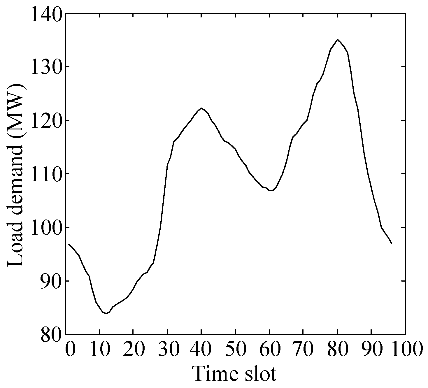
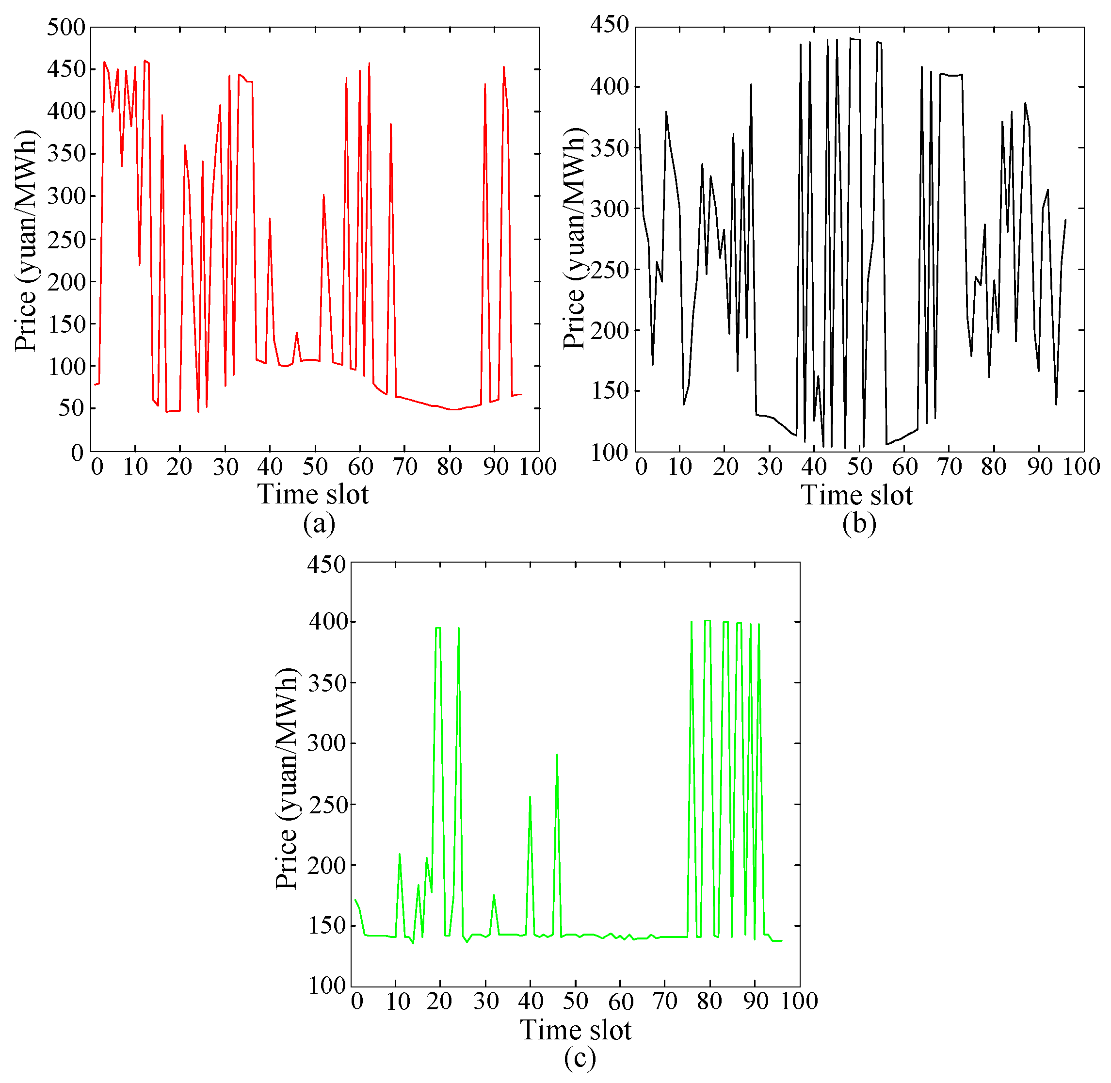
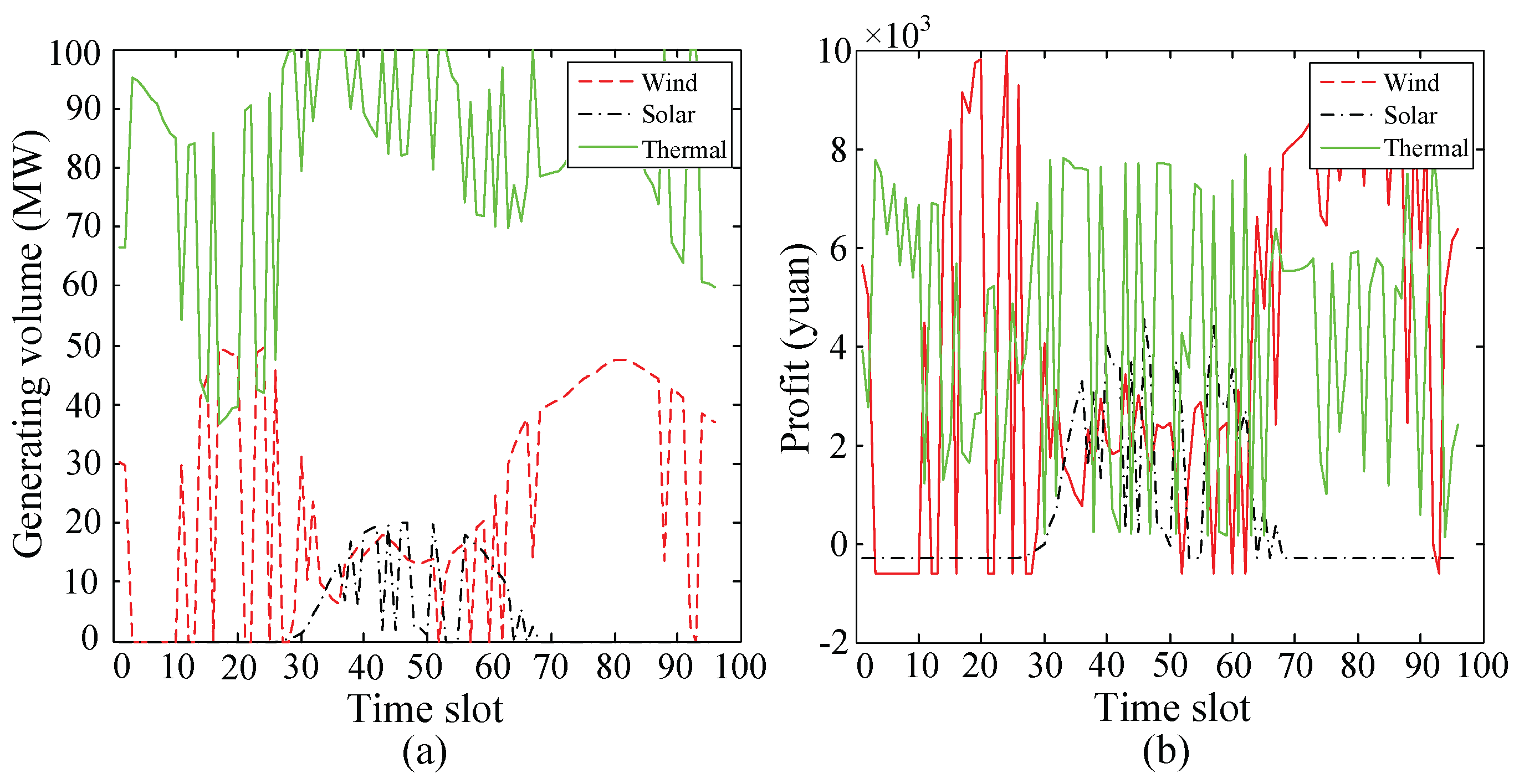
5. Numerical Results

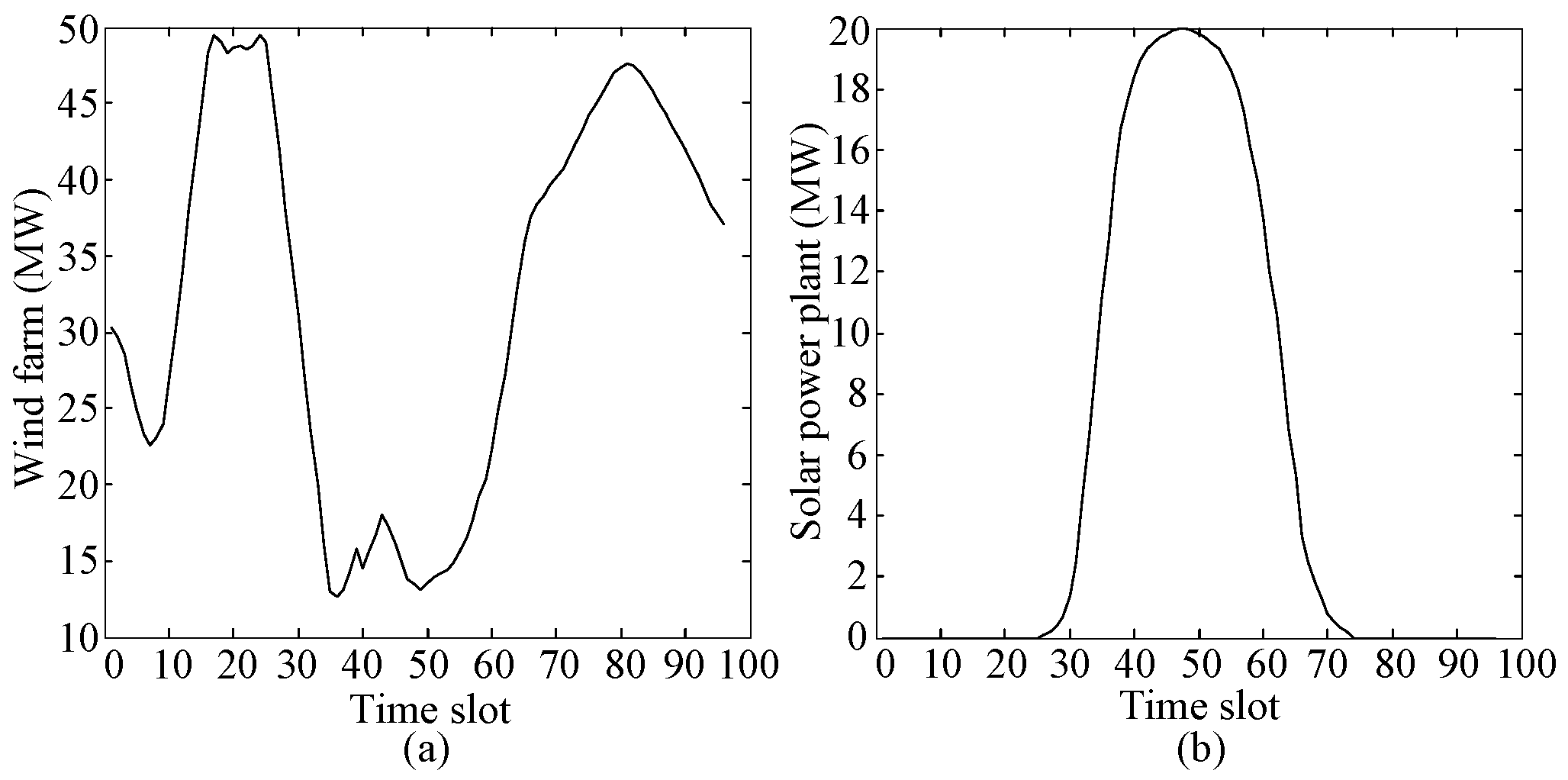
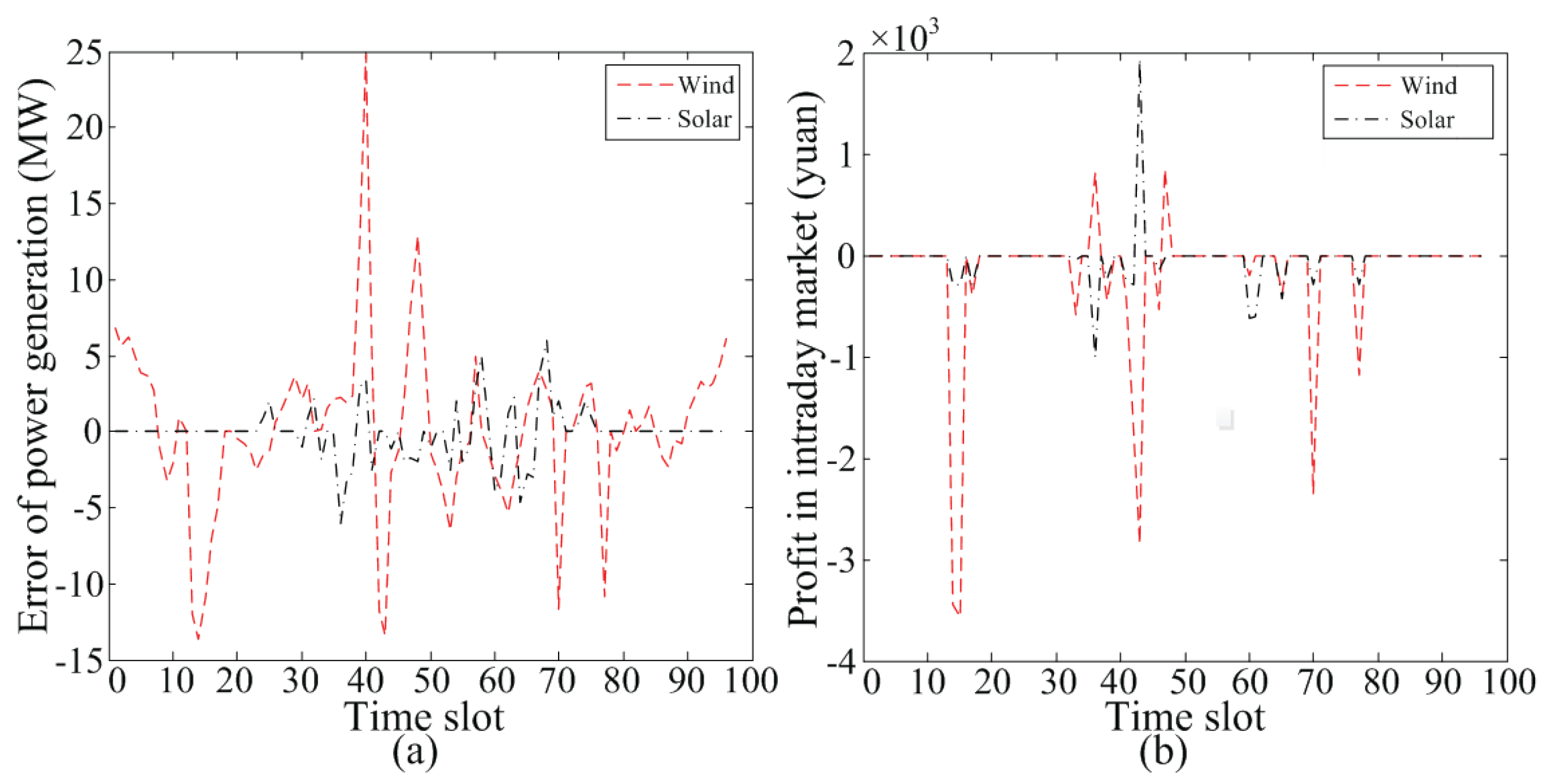
5.1. Simulations

In this section, several simulations will be presented to illustrate the feasibility of the presented method for bi-level optimization based on the non-cooperative game in a competitive electricity market. Assume that $N=$ 3 in Figure 1, and the three power plants are a wind farm, a solar power plant and a thermal power plant, respectively.

Table 1. Generation parameters of power plants.

Power Plants	Installed Capacity (MW)	${\mathit{a}}_{\mathit{n}}$ (Yuan/MWh2)	${\mathit{b}}_{\mathit{n}}$ (Yuan/MWh)	${\mathit{c}}_{\mathit{n}}$ (Yuan)	Minimum Output (MW)
Wind farm	49.5	0	0.018	2490	0
Solar power plant	20	0	0.023	1187	0
Thermal power plant	100	0.063	125.3	0	20

,

Table 2. Price parameters of power plants.

Power Plant	${\mathit{b}}_{\mathbf{nb}min}$ (Yuan)	${\mathit{b}}_{\mathbf{nb}max}$ (Yuan)	${\mathit{p}}_{\mathbf{ns}}$ (Yuan/MWh)	${\mathit{a}}_{\mathbf{nb}}$ (Yuan/MWh)
Wind farm	130	460	215	−1.6945
Solar power plant	130	510	420	−1.35468
Thermal power plant	130	390	0	0.126

and

Table 3. System parameters.

${\mathit{p}}_{\mathbf{cr}}$ (Yuan/MWh)	${\mathit{p}}_{\mathbf{ct}}$ (Yuan/MWh)	$\mathit{\sigma }$	$\mathit{\mu }$ (t/MWh)	${\mathit{k}}_{\mathit{f}}$
190	190	0	1.3	1.1

and Figure 2 and Figure 3 all are input parameters for the simulations. Several parameters for three power plants are presented in Table 1 and Table 2, and some of them have been adopted from [25] with some modifications. In Table 1, $a_n$, $b_n$, $c_n$ denote fixed parameters of the total generation cost of power plants, and $n=1,2,3$ denote the wind farm, solar power plant and thermal power plant, respectively. Additionally, the quadratic coefficient of total generation cost is zero for the wind farm and solar power plant, because their generation cost is linear. A regional grid is considered in this paper, and system parameters are shown in Table 3. Figure 2 is the daily load demand curve of all utility companies, and the predictive generating volume of the wind farm and solar power plant are shown in Figure 3.

Simulation results on the day-ahead market are shown in Figure 4 and Figure 5 and

Table 4. Profit of power producers in the day-ahead market.

Power Plant	Profit (${10}^4$ Yuan)	Trading Generating Volume (MWh)	Maximum Generating Volume (MWh)
Wind farm	37.91	563.73	773.37
Solar power plant	5.35	88.83	136.1
Thermal power plant	42.09	1956.93	2400

. Figure 4 shows the bidding price of the wind power producer, solar power producer and thermal power producer at 96 time slots. Profit and cleared generating volume of the wind power producer, solar power producer and thermal power producer at each time slot on the day-ahead market are shown in Figure 5. According to Figure 5a, note that the cleared generating volume of the wind power producer and solar power producer at some time slots is zero. High capital cost puts them at a disadvantage in the power generation competition. From Figure 5b, one can see that the profit of the wind power producer and solar power producer has a negative value at some time slots, while the profit of the thermal power producer is positive all of the time. Because the cleared generating volume of the wind farm and solar power plant is zero sometimes, it means that the wind power producer and solar power producer cannot capture profit by generating electricity, while the fixed generation cost still exists. Profit on the day-ahead market for three power producers in a whole day are listed in Table 4. One can see that not only the thermal power producer, but the wind power producer and solar power producer can obtain substantial gains, because the carbon emission and subsidy for new energy power plant factors are considered.

In the intraday market, the difference between the generating volume produced during the real-time operation and scheduled in the day-ahead market is shown in Figure 6a, which are the input parameters. Figure 6b shows the simulation results on the profit of the wind power producer and solar power producer on the intraday market. The profits of the wind power producer and solar power producer are negative, due to the fines, when $q_{wp}$ is less than $q_{wD}$ or $q_{sp}$ is less than $q_{sD}$ and the difference is in excess of 8%. One has to notice that the wind power producer and solar power producer still can make profits on the intraday market. Total profits both in the intraday market and day-ahead market are shown in

Table 5. Profit of the power producers in the intraday market.

Power Plant	Profit (${10}^4$ Yuan)	Total Profit (${10}^4$ Yuan)
Wind farm	−2.65	35.26
Solar power plant	−0.61	4.74
Thermal power plant	0.14	42.23

. Renewable energy power producers still can make a good profit even though fines need to be paid for the uncertainty of power generation.

5.2. Discussions

If the wind power producer and solar power producer are not participating in the intraday market, they need to buy electricity in the reserve market or real-time market when the practical generating volume is less than the cleared generating volume on the day-ahead market and the difference is in excess of eight percent. Additionally, the thermal power producer cannot obtain extra profit in the reserve market, which is selected in this case. System parameters are the same as the previous case on the intraday market in Section 5.1, and the reserve price is 224.8 $/MWh [14]. Total profits for three power producers during a whole day with participation in the reserve market are shown in

Table 6. Profit of power producers in the reserve market.

Power Plant	Profit in Reserve Market (${10}^4$ Yuan)	$\mathbf{\Delta }{\mathit{P}}_{\mathit{n}}$ (${10}^4$ Yuan)
Wind farm	−5.03	2.38
Solar power plant	−1.53	0.92
Thermal power plant	0	0.14

. $\Delta P_n$ denotes the difference of the cost between scheduling with the intraday market and the reserve market. One can see that the profits of all power producers with participation in the intraday market are higher than the cost without participating in the intraday market.

The interior point method utilized by power plants to maximize profit is simulated in this part. System parameters in this case are the same as Section 5.1 in the day-ahead market. For the above three power producers, simulation results on the day-ahead market, which use the interior point method without game, are shown in

Table 7. Daily profit of power producers using different methods in the day-ahead market (${10}^4$ yuan).

Power Plant	No Game	With Game	$\mathbf{\Delta }{\mathit{P}}_{\mathit{gn}}$
Wind farm	37.29	37.91	0.62
Solar power plant	5.28	5.35	0.07
Thermal power plant	42.02	42.09	0.07
All power plants	84.59	85.35	0.76

. From Table 7, one can see that the profits of all power plants are reduced compared to using game theory, where $\Delta P_{gn}$ denotes the difference of profit between scheduling with and without the game in the day-ahead market. Besides, when the wind farm, solar power plant and thermal power plant do not apply the non-cooperative game, their profits are decreased by 1.66%, 13.3% and 1.67%, respectively. Consequently, the total profit of three power plants using the interior point method is smaller than of the ones participating in the game.

6. Conclusions

This paper presents a scenario in a competitive electricity market having multiple power producers, multiple utility companies, a PX and an ISO. A non-cooperative game approach-based bi-level optimization is proposed, where power producers are at the upper level and utility companies are at the lower level. In addition, strategies of the non-cooperative game are the bidding strategies of power producers. A distributed algorithm is presented to realize the optimization in terms of maximizing the profit of all power producers. Numerical simulations were carried out to show the effectiveness and feasibility of the proposed scheme and algorithm. Simulation results show that all power producers can benefit from the game: (1) not only the thermal power producer, but also the wind power producer and solar power producer can benefit by participating in the non-cooperative game-based bi-level optimization; (2) the wind farm and solar power plant are able to transmit substantial generating volume, which is helpful for renewable energy accommodation.

The optimization model in this paper can be enhanced further in mainly two respects: the existence and uniqueness of the equilibrium solution for the proposed non-cooperative game-based bi-level optimization approach still is an open problem, and competition among utility companies is ignored, which can be carried out in future work.

References

1. Gountis, V.P.; Bakirtzis, A.G. Bidding strategies for electricity producers in a competitive electricity marketplace. IEEE Trans. Power Syst. 2004, 19, 356–365. [Google Scholar] [CrossRef]
2. Woo, C.K.; Lloyd, D.; Tishler, A. Electricity market reform failures: UK, Norway, Alberta and California. Energy Policy 2003, 31, 1103–1115. [Google Scholar] [CrossRef]
3. Sharma, K.C.; Bhakar, R.; Tiwari, H.P. Strategic bidding for wind power producers in electricity markets. Energy Convers. Manag. 2014, 86, 259–267. [Google Scholar] [CrossRef]
4. Morales, J.M.; Conejo, A.J.; Perez-Ruiz, J. Short-term trading for a wind power producer. IEEE Trans. Power Syst. 2010, 25, 554–564. [Google Scholar] [CrossRef]
5. Fampa, M.; Barroso, L.A.; Candal, D.; Simonetti, L. Bilevel optimization applied to strategic pricing in competitive electricity markets. Comput. Optim. Appl. 2008, 39, 121–142. [Google Scholar] [CrossRef]
6. Zhang, G.; Zhang, G.; Gao, Y.; Lu, J. Competitive strategic bidding optimization in electricity markets using bi-level programming and swarm technique. IEEE Trans. Ind. Electron. 2011, 58, 2138–2146. [Google Scholar] [CrossRef]
7. Pang, J.S.; Fukushima, M. Quasi-variational inequalities, generalized Nash equilibria, and multi-leader- follower games. Comput. Manag. Sci. 2005, 2, 21–56. [Google Scholar] [CrossRef]
8. Bathurst, G.N.; Weatherill, J.; Strbac, G. Trading wind generation in short term energy markets. IEEE Trans. Power Syst. 2002, 17, 782–789. [Google Scholar] [CrossRef]
9. Matevosyan, J.; Soder, L. Minimization of imbalance cost trading wind power on the short-term power market. IEEE Trans. Power Syst. 2006, 21, 1396–1404. [Google Scholar] [CrossRef]
10. Pinson, P.; Chevallier, C.; Kariniotakis, G.N. Trading wind generation from short-term probabilistic forecasts of wind power. IEEE Trans. Power Syst. 2007, 22, 1148–1156. [Google Scholar] [CrossRef]
11. Bridier, L.; David, M.; Lauret, P. Optimal design of a storage system coupled with intermittent renewables. Renew. Energy 2014, 67, 2–9. [Google Scholar] [CrossRef]
12. Ghaffari, R.; Venkatesh, B. Options based reserve procurement strategy for wind generators—Using binomial trees. IEEE Trans. Power Syst. 2013, 28, 1063–1072. [Google Scholar] [CrossRef]
13. Abreu, L.V.; Khodayar, M.E.; Shahidehpour, M.; Wu, L. Risk-constrained coordination of cascaded hydro units with variable wind power generation. IEEE Trans. Sustain. Energy 2012, 3, 359–368. [Google Scholar] [CrossRef]
14. Dai, T.; Qiao, W. Trading wind power in a competitive electricity market using stochastic programing and game theory. IEEE Trans. Sustain. Energy 2013, 4, 805–815. [Google Scholar]
15. Zugno, M.; Morales, J.M.; Pinson, P.; Madsen, H. Pool strategy of a price-maker wind power producer. IEEE Trans. Power Syst. 2013, 28, 3440–3450. [Google Scholar] [CrossRef]
16. Baringo, L.; Conejo, A.J. Strategic offering for a wind power producer. IEEE Trans. Power Syst. 2013, 28, 4645–4654. [Google Scholar] [CrossRef]
17. Dai, T.; Qiao, W. Optimal bidding strategy of a strategic wind power producer in the short-term market. IEEE Trans. Sustain. Energy 2015, 6, 707–719. [Google Scholar] [CrossRef]
18. Kazempour, S.J.; Zareipour, H. Equilibria in an oligopolistic market with wind power production. IEEE Trans. Power Syst. 2014, 29, 686–697. [Google Scholar] [CrossRef]
19. Dai, T.; Qiao, W. Finding equilibria in the pool-based electricity market with strategic wind power producers and network constraints. IEEE Trans. Power Syst. 2017, 32, 389–399. [Google Scholar] [CrossRef]
20. Kristiansen, T. A time series spot price forecast model for the Nord Pool market. Int. J. Electr. Power Energy Syst. 2014, 61, 20–26. [Google Scholar] [CrossRef]
21. Skajaa, A.; Edlund, K.; Morales, J.M. Intraday trading of wind energy. IEEE Trans. Power Syst. 2015, 30, 3181–3189. [Google Scholar] [CrossRef]
22. Fang, X.; Li, F.; Wei, Y.; Azim, R.; Xu, Y. Reactive power planning under high penetration of wind energy using Benders decomposition. IET Gener., Transm. Distrib. 2015, 9, 1835–1844. [Google Scholar] [CrossRef]
23. Zhang, H.; Gao, F.; Wu, J.; Liu, K.; Zhai, Q. A stochastic Cournot bidding model for wind power producers. In Proceedings of the IEEE International Conference on Automation and Logistics, Chongqing, China, 15–18 August 2011; pp. 319–324. [Google Scholar]
24. Sharma, K.C.; Bhakar, R.; Padhy, N.P. Stochastic cournot model for wind power trading in electricity markets. In Proceedings of the Power and Energy Society General Meeting, National Harbor, MD, USA, 27–31 July 2014; pp. 1–5. [Google Scholar]
25. Zhao, Z.Y.; Li, Z.W.; Yao, X. Study on cost price of wind power electricity based on the certified emission reduction income. Renew. Energy Resour. 2014, 32, 662–667. (In Chinese) [Google Scholar]
26. Gan, L.; Eskeland, G.S.; Kolshus, H.H. Green electricity market development: Lessons from Europe and the US. Energy Policy 2007, 35, 144–155. [Google Scholar] [CrossRef]
27. Sorknaes, P.; Andersen, A.N.; Tang, J.; Strom, S. Market integration of wind power in electricity system balancing. Energy Strategy Rev. 2013, 1, 174–180. [Google Scholar] [CrossRef]
28. Robinson, M. Role of balancing markets in wind integration. In Proceedings of the IEEE PES Power Systems Conference and Exposition, Atlanta, GA, USA, 29 October–1 November 2006; pp. 232–233. [Google Scholar]
29. Hu, X.; Ralph, D. Using EPECs to model bi-level games in restructured electricity markets with locational prices. Oper. Res. 2007, 55, 809–827. [Google Scholar] [CrossRef]
30. Ghotbi, E.; Dhingra, A.K. A bi-level game theoretic approach to optimum design of flywheels. Eng. Optim. 2012, 44, 1337–1350. [Google Scholar] [CrossRef]
31. Haghighat, H.; Seifi, H.; Kian, A.R. Gaming analysis in joint energy and spinning reserve markets. IEEE Trans. Power Syst. 2007, 22, 2074–2085. [Google Scholar] [CrossRef]
32. Song, H.; Liu, C.C.; Lawarree, J. Nash equilibrium bidding strategies in a bilateral electricity market. IEEE Trans. Power Syst. 2002, 17, 73–79. [Google Scholar] [CrossRef]
33. Wu, H.; Shahidehpour, M.; Alabdulwahab, A.; Abusorrah, A. A game theoretic approach to risk-based optimal bidding strategies for electric vehicle aggregators in electricity markets with variable wind energy resources. IEEE Trans. Sustain. Energy 2016, 7, 374–385. [Google Scholar] [CrossRef]
34. Hobbs, B.F.; Metzler, C.B.; Pang, J.S. Strategic gaming analysis for electric power systems: An MPEC approach. IEEE Trans. Power Syst. 2000, 15, 638–645. [Google Scholar] [CrossRef]
35. Leyffer, S.; Munson, T. Solving multi-leader-common-follower games. Optim. Methods Softw. 2010, 25, 601–623. [Google Scholar] [CrossRef]
Figure 1. Generation side bidding transaction model.
Energies 10 00627 g001
Figure 2. Daily load demand of all utility companies.
Energies 10 00627 g002
Figure 3. Predictive generating volume: (a) wind farm; (b) solar power plant.
Energies 10 00627 g003
Figure 4. Bidding price on the day-ahead market: (a) wind farm; (b) solar power plant; (c) thermal power plant.
Energies 10 00627 g004
Figure 5. Power producers on the day-ahead market: (a) cleared generating volume; (b) profit.
Energies 10 00627 g005
Figure 6. Simulation parameters and results in the intraday market: (a) difference between generating volume produced during the real-time operation and that scheduled in the day-ahead market; (b) profit of power producers in the intraday market.
Energies 10 00627 g006