
Effects of Building Occupancy on Indicators of Energy Efficiency


VTT Technical Research Centre of Finland Ltd., Espoo, FI-02044 VTT, Finland
*
Author to whom correspondence should be addressed.
Energies 2017, 10(5), 628; https://doi.org/10.3390/en10050628
Submission received: 3 March 2017
/
Revised: 18 April 2017
/
Accepted: 27 April 2017
/
Published: 4 May 2017
Abstract
:The potential to reduce energy consumption in buildings is high. The design phase of the building is very important. In addition, it is vital to understand how to measure the energy efficiency in the building operation phase in order to encourage the right efficiency efforts. In understanding the building energy efficiency, it is important to comprehend the interplay of building occupancy, space efficiency, and energy efficiency. Recent studies found in the literature concerning energy efficiency in office buildings have concentrated heavily on the technical characteristics of the buildings or technical systems. The most commonly used engineering indicator for building energy efficiency is the specific energy consumption (SEC), commonly measured in kWh/m2 per annum. While the SEC is a sound way to measure the technical properties of a building and to guide its design, it obviously omits the issues of building occupancy and space efficiency. This paper studies existing energy efficiency indicators and introduces a new indicator for building energy efficiency which takes into account both space and occupancy efficiency.
1. Introduction
According to the International Energy Agency (IEA), 9% of the world’s energy is consumed in commercial buildings, contributing a total of 12% of global CO2 emissions, either directly or indirectly [1,2]. The potential for energy savings and emission reductions is major. Considering buildings in general, the Intergovernmental Panel on Climate Change (IPCC) [3] and the European Commission [4] are among the latest organizations to uncover the greatest energy saving potentials in buildings compared to other sectors of the economy. These results were lately further corroborated by the industry’s own findings, published by the World Business Council for Sustainable Development [5]. Concerning commercial buildings specifically, a review of studies by U.S. Department of Energy [6] found technical potentials of 12.0–40.4% and economic potentials of 10.8–34.3% for energy efficiency improvements in typical buildings.
In understanding the building energy efficiency, it is important to comprehend the interplay of building occupancy, space efficiency, and energy efficiency in office buildings, with a focus on indicators. Recent studies found in the literature concerning energy efficiency in office buildings have concentrated heavily on the technical characteristics of the buildings or technical systems. The most commonly used engineering indicator for building energy efficiency—called the specific energy consumption (SEC), commonly measured in kWh/m2 per annum—also appears as the most common indicator in the literature reviewed for this study. This paper aims to show how the commonplace use of SEC alone is problematic in the context of varying true occupancy profiles. While it is a sound way to measure the technical properties of a building and to guide its design, it obviously omits the issues of building occupancy and space efficiency. In fact, the higher the occupancy and space efficiency, the less efficient the building tends to appear using SEC, because the components of energy use that are dependent on the amount of users are higher, while the floor area of the building stays constant [7,8].
In recent literature, Mendes et al. [9] compared the energy efficiency of Chinese and American case office buildings, Chung and Hui [10] studied the energy efficiency in offices in Hong Kong, Pikas et al. [11] calculated cost optimal zero energy building solutions for office buildings, Zhao et al. [12] studied the effect of supervision on the energy efficiency of office buildings in China, Boyano et al. [13] estimated the energy saving potentials in European case offices, and Nunes et al. [14] compared the energy efficiency in two Portuguese case offices, with all electing to use the SEC as the main indicator. Two of these studies [12,14] included occupancy and space use in their scope and from these, Nunes et al. [14] attempted to take into account space efficiency in indicators by introducing what they call energy efficiency index per standard occupants (EEIREAL,OCC), where the building energy use is divided by the normalized amount of occupants in the building. It has also recently been suggested that studies should adjust energy consumption benchmarks to longer operation times of the building [15] or a higher space efficiency [16], but the correlations are not straightforward [17,18].
Similar approaches to account for the effects of occupancy on energy efficiency indicators have been suggested by Forsström et al. [19], where the SEC is adjusted for the utilization rate of the building (SECO) and an indicator called the energy intensity of usage (EIU), meaning the energy use of the building divided per capita. In [7], alongside the SEC and EIU, a similar type of indicator to that is shown in [19], where (SECO) is proposed by dividing the energy per area by the occupied hours (SECIO). Variations of indicators taking into account occupancy or space efficiency are presented in [20]. For such indicators to be used, it is critical to find out how to monitor the occupancy levels in a building in a reliable way. Building occupancy is hard to monitor in a reliable and exact way, and the estimations that can be found in the literature often rely only on facility managers’ observations or surveys that might present inaccurate results.
1.1. Measuring Energy Efficiency
Traditionally, energy efficiency is expressed in kWh/m2. It is an appropriate indicator to evaluate the energy efficiency when considering the physical properties of the building in the design phase. However, it is a purely technical indicator that omits the utility of the energy provided; particularly the amount of users it serves. Therefore, there is no linear correlation between the technical calculated energy efficiency in kWh/m2 and the actual measured energy efficiency encompassing the effects of occupants in the building. In the design phase, the operational energy consumption is typically simulated by using standard occupancy schedules [21]. However, those only provide a poor estimate of the real occupancy measured in the operation (there is a 46% difference between the American Society of Heating, Refrigerating and Air-Conditioning Engineers ASHRAE standardized occupancy used in the simulation and the real occupancy according to Duarte et al. [22]). Operational energy consumption is affected by lighting, plug loads, heating, ventilation and air conditioning equipment utilization, fresh air requirements, and internal heat gain/loss, which depend on the number of occupants and their behavior. However, the latter are not well known in advance and are difficult to capture during the operation [21]. It is therefore not surprising that a significant discrepancy between the predicted and actual energy consumption is often observed (on average, a 34% increase in a study [23] consisting of 62 case study buildings, with the dominant root causes for the performance gap being specification uncertainty in modeling, occupant behavior, and poor operational practices). In addition, the occupants often don’t know how to use the building as intended in the design, which can also explain the lower measured energy efficiency than expected. The study of Karjalainen [24] shows that 75% energy savings can be achieved with users with careless energy consuming behavior by using a robust design that is less sensitive to occupant behavior. On the other hand, energy savings can be achieved in the operation phase by properly matching the energy supply with demand. This, however, requires that there is real time knowledge available on building occupancy levels, and that intelligent building automation and demand control systems are available. Most modern buildings today typically condition rooms assuming a maximum occupancy, instead of the actual occupancy. Ericson et al. [25] show a potential for 42% energy savings using real time occupancy data based on sensor network occupancy model prediction strategies, while still maintaining ASHRAE comfort standards. In a study of Taylor [26], over 10% energy cost savings are achieved by matching the energy consumption with occupancy in a naval air station consisting of 280 buildings.
While kWh/m2 is a useful metric when comparing a building’s physical properties in the design phase, it can favour unsustainable ways of utilising buildings in the operation phase. As a matter of fact, a lower space efficiency (m2/person), shorter operating times of buildings (per day, per week, per year), or a lower level of the presence of occupants can lead to a situation where such buildings seem more energy efficient in kWh/m2 than a building which is utilised more efficiently, while the physical properties of the buildings are similar. This effect was shown in [7], which compared the energy efficiency with three indicators (SEC, EIU, and SECIO) for the different space efficiencies and daily operating times of an office building through energy simulations. When SEC was used, it appeared that the energy efficiency decreased slightly when the office layout became more efficient. However, with the two latter indicators, the effect was the complete opposite. When the daily operating times were varied, SEC favoured shorter working hours per day, while the two other indicators were considered more energy efficient when the building was used for a longer period of time per day.
In rewarding schemes for energy consumption, the ability to compare one’s own consumption to that of peers, is a powerful method. A school or hospital should not be penalised for having longer operating times than another that uses a similar building of the same size. Similarly, an organisation shouldn’t be punished for having an especially efficient office layout. Therefore, the functional unit should not be only square meter when comparing the energy consumption of a six-person family to that of a single person occupying a similar building.
1.2. Meaning of Building Occupancy
The efficiency of building usage is affected by space efficiency measured in [m2/person] and building occupancy. Building occupancy is affected by the operating times (number of daily hours, weekly days, and yearly days) and occupancy levels (percentage of occupants present at a given moment). Thus, building occupancy can be calculated as a multiplication of yearly operating times and average occupancy levels, or by counting the total person hours (sum of hours each building occupant has spent in the space studied). Usually, space efficiency is preliminary fixed in the design phase and the operating times of the buildings are fixed based on the purpose of the building. The occupancy levels, however, have to be monitored, which is currently not easy to do in a reliable and cheap way (for most advanced existing methods, see for example [27]).
Space efficiency is affected by space design and office layout. There are a wide range of different work settings and office layouts, from traditional office rooms to open-plan offices and hot-desks with non-allocated workstations. New ways of working—which are characterised by collaborative workspaces, virtual and remote work, and unclear notions of workplace and work time—put the space needed into a new perspective. According to [28], space efficiency is almost directly correlated with the energy consumption of an organisation in refurbishments. The more effectively a given building is occupied, the less space is needed for a given number of people and the lower the space heating energy consumption per person. However, in cooling periods, the space efficiency might increase the cooling demand. The same applies to the operating times of a building; it can have several purposes at different times of day (e.g., organisation of leisure activities in a school after normal school hours). Better real time knowledge on building occupancy helps to operate the building automation systems more intelligently and to save energy used for ventilation and lighting. However, the more effectively a given space is used, the more it consumes in absolute numbers, and the less energy efficient the building is if the efficiency is measured in kWh/m2.
The objective of this paper is to test the feasibility of indicators that take into account how efficiently a building is used. In this paper, the use of different indicators in case buildings from Finland is examined. The aim of the study is to find out the strengths and weaknesses of the different alternative indicators and to provide a recommendation for a combined appraisal of occupancy and energy efficiency, with the help of suitable indicators in different phases of the construction process and building maintenance.
2. Methods
The purpose of this paper is to compare different alternative indicators of energy efficiency with regard to their feasibility, advantages, and disadvantages. The analyzed indicators are presented in Table 1 of Section 2.1, and try to capture the efficiency of building use, in addition to the technical aspects covered with the traditional energy efficiency indicator kWh/m2. The analyzed indicators have different data requirements for estimating the relations between energy consumption, space efficiency, and building occupancy. This paper uses a mixture of five case studies with different methods to evaluate the data, in order to illustrate the level of difficulty of collecting the needed data in different types of situations. This approach also allows an analysis of which indicators are the most appropriate.
Case study 1 focuses on the methods used to measure building occupancy in a reliable way. Case study 2 focuses on evaluating the effect of occupancy on energy consumption through energy simulation. Further, case study 3 focuses on the interplay between the measured actual occupancy and energy consumption. Finally, case studies 4 and 5 use existing buildings that will be renovated, with the aim of improving both the energy efficiency and space efficiency. Their renovation plan is used as a starting point for calculating the situation after the renovation, but with assumptions for both the energy and space use efficiency improvements.
Section 2.2 presents the case buildings used in the five case studies. The methods used to assess building occupancy are presented in Section 2.3. The calculation methods used in cases 4 and 5 are explained in Section 2.4, and the simulation method used in case 2 is presented in Section 2.5.
2.1. Indicators
This paper evaluates the different possibilities for indicating energy efficiency. For this purpose, different indicators are tested in five case studies. The indicators express the annual energy consumption of a building with different functional units. The most typical functional unit is the unit of space, i.e., m2. Such an indicator might be penalised for efficient space use, and therefore, it is compared to indicators that account for the number of people using the building and their presence in the building. The studied indicators are presented in Table 1.
2.2. Case Buildings
This section presents the case buildings used in the five case studies, with each building being numbered with the associated case study from 1 to 5. All the case buildings are office buildings, except building 4, which is an educational building.
2.2.1. Case Building 1
The case building is a conventional office building with three floors in Helsinki, Finland, used by a consulting company.
2.2.2. Case Building 2
Case building 2 is a simulation case where the effects of building occupancy on energy consumption are simulated. The building that was modelled for the simulations represents a conventional office building in Helsinki. It has five floors with a total floor area of 4123 m2 and 310 workers, of which 75% work in open-plan offices with 12 m2/person and 25% work in office rooms with 17 m2 per person. Thus, the average space efficiency is 13.3 m2/person.
2.2.3. Case Building 3
The case building is a conventional office building with four floors in Espoo, Finland. The selected space for the case study includes workstations for 37 persons, of which 25 are in personal or shared office rooms and 12 are in an open-plan office. The space efficiency in the studied space was 9.9 m2/person on average.
2.2.4. Case Building 4
This educational case building was built in the year 1969. The building is due to be renovated, since the facade and some technical systems have reached the end of their life time. In addition, the renovation plan includes a different space layout with a more open space and less single person office rooms. Moreover, some laboratories will be merged. The gross floor area of the building is 10,161 m² and the volume of the building is 39,100 m³. The main functions and their floor areas are shown in Table 2. The building has two underground storeys and four storeys above the ground. The building is quadratic in form and the major facades face towards northeast and northwest. The building has a mechanical ventilation system without heat recovery. Space heating is mainly carried out with a nozzle convector underneath the windows. Originally, the system also had a cooling option, but that was disabled 20 years ago. Due to discomfort in the thermal environment, some rooms have additional electrical heaters. Space cooling was installed in rooms facing northeast and in some specific laboratories.
2.2.5. Case Building 5
This office building was built in the year 1965, but it has been renovated quite recently during the 2000’s. The renovation included a modernization of the ventilation system and a retrofitting of a cooling system. Now, a new renovation is planned to implement changes in the use of the building. Currently, the building houses multiple organizations, but after the renovation, it is planned that one of the organizations will occupy the entire building, moving in some of its personnel from other locations. It is planned that after the renovation, the space use efficiency of the organization will be higher, meaning that the same functions will be produced in a smaller amount of space, without a loss of comfort. During the renovation, the inner walls and spaces in the building will be modified. The total area to be renovated is 2500 m². The main functions and floor areas are shown in Table 3.
2.3. Methods to Assess the Building Occupancy
2.3.1. Case 1
This case study consisted of monitoring occupancy levels in a selected zone of building 1 during one week in October 2012. Seventeen building occupants participated in the study, 12 of which were in an open-plan office with 7 m2/person and five of which occupied personal office rooms (10 m2/person). Three different methods were used simultaneously to monitor the occupancy levels, in order to ensure the reliability of the results and to identify any possible incorrect results when using particular methods.
(1) Occupancy measurements with Wirepas technology
The participants carried wireless occupancy tracking badges (produced by Wirepas) when they were in the building. This technology detects a person’s presence with the help of Wi-Fi-based receptors installed in the workspaces. The results were analysed with the space optimisation tool Optimaze Active [30] that illustrates one hour averages of occupancy levels. Based on the results, the software gives a recommendation on the amount of workstations required for the given number of workers. In order to be reliable, it is important that the users remember to carry their badge whenever they are in the building. In this study, special attention was paid to instructing and reminding the participants to carry the badges.
(2) Surveys
All the participants filled in a survey on their presence, in which they indicated the following information every day: arrival time to workplace; leaving time from workplace; absences from workplace with indication of time, duration, and reason (e.g., business trip, sickness, remote work, meeting, lunch, personal); and absences from workstation of more than 15 min with an indication of time, location, duration, and reason. The participants were not asked about their satisfaction with the indoor environment and they did not have the possibility to adjust those conditions.
(3) Walktroughs and observations
One of the authors of this article was present in the case area during the whole duration of the experiment. This was important in order to ensure that the participants carried the badges correctly and filled in the surveys. In addition, three to four walkthroughs per day were carried out (manually counting the persons present) to be able to verify the reliability of the other methods used to monitor the occupancy levels. The participants were informed about the aims of the study to improve the working environment and were assured that, e.g., no one would be penalised for any absences, and that the only important aspect was to fill in the surveys carefully, so that the results would be reliable.
2.3.2. Case 2
In case study 2, three different occupancy profiles were used to simulate the effect of occupancy on energy consumption. The occupancy profiles are presented later in Figure 3.
2.3.3. Case 3
This case study consisted of monitoring the occupancy levels and people-related electricity consumption in a selected zone of case building 3 in November 2013 on an hourly level during one week and based on measured data. The hourly electricity consumption was manually read from the space specific electricity meter and the occupancy levels were counted manually on an hourly basis by simultaneous walk-throughs.
2.3.4. Cases 4 and 5
For the element concerning the amount of people, the study relied on questionnaires in which the employees estimated their presence in various parts of the building during a typical week. For the office, this did not include the clients that visited the building, and for the educational building, students were excluded. In the office, the effect of clients was not major because the space available to them took up a very small share of the building. Therefore, their effect on the building’s energy consumption was minor and did not affect the topic studied in a major way. The absence of students from the numbers available for the educational building is problematic. Therefore, two accounts of the results are offered here: one for the whole building and another for the workspaces that are only accessible to the employees. This is done to demonstrate how problems that are frequently encountered by people analysing building occupancy and energy use can be taken into account when interpreting the results.
2.4. Calculation Methods for Cases 4 and 5
In the calculations, the situation before the renovation was used as a base case. The renovation plan was used as a starting point for calculating the situation after the renovation, but with assumptions for both the energy and space use efficiency improvements. When the space use efficiency was increased, it was assumed that the electricity consumption per floor area increased due to the higher density of appliances.
Only rather generalized energy measurements were available from the meters in the old building. Moreover, only the total figures for heating, including domestic hot water and space heating, and electricity and cooling could be read. Additionally, cold water consumption was measured. In order to find out the room-specific SECs, previous material and literature were used to estimate the energy use in the different spaces.
The energy measurements were very rough, since the building was old. No detailed energy measurements were conducted, and only the numbers for heating, including domestic hot water and space heating, and electricity and cooling could be logged from the meters. Additionally, cold water consumption was measured. In order to find out the room SECs, previous material and literature were used to quantify the energy use in different types of spaces. Referring to [31], the average energy consumption numbers for some types of spaces are shown in Table 4.
On the other hand, according to the results of a survey by [32], the average thermal load is 456.3 kWh/m²/a and the electricity load is 457.5 kWh/m²/a for a laboratory space. Together with the values from [31], these were used to calculate the estimated energy consumption in various spaces in the case buildings. The calculation was made so that the relative energy consumption in different room types was kept the same as [31,32] suggest, but the numbers were scaled so that the total known energy consumption from the building would match with the estimate.
2.5. Simulations Methods for Case 2
Based on the measured occupancy levels from the office building case 1, the effects of occupancy on energy consumption were simulated for case building 2 with different occupancy profiles.
The effects of occupancy levels on energy consumption were simulated during one year with different occupancy profiles with the dynamic thermal simulation tool IDA indoor climate and energy (IDA-ICE) [33]. In contrast to traditional monolithic simulation codes, IDA-ICE is based on symbolic equations in a general modeling language and uses a variable time step differential-algebraic (DAE) solver.
IDA-ICE is a well validated whole-year detailed and dynamic multi-zone simulation application for the study of thermal indoor climate, as well as the energy consumption of an entire building. The physical models of IDA-ICE reflect the latest research and best models available. The models are written in neutral model format (NMF) or Modelica, which serve as a readable document and a computer code. Via translators, the models can be used in several modular simulation environments [34,35].
3. Results
3.1. Case Study 1
In order to analyse the reliability of the three different methods (wirepas measurements, surveys, and manual counting in walk-throughs), the results from the three to four daily walkthroughs (total 17) are compared to the results from the surveys and measurements.
The results from the different methods are compared in Figure 1 for one day. It is to be noted that a certain difference between the three results is logical, because the manual counting gives an accurate momentary result, while the two other results are one hour averages. Another question associated with the methods is whether the people are counted as present if there is clear evidence of their presence (lights and computer on) while they are not physically at their workstation, but are probably in the building. In the surveys, the location was requested and people were counted present if they were on the same floor. In the walk-throughs, people were counted as present if there was clear evidence of their presence, even if they were not at their workstation. The Wirepas device counts a person present if (s)he is in the area of the study. However, if (s)he is in a meeting room, (s)he is counted in a different category.
The median of the difference between the hourly averaged survey results and the walk-throughs is 0, and the average difference is 0.6 persons. For the Wirepas measurements compared to the walk-throughs, the median of the difference is 1 person and the average difference is 1.6 persons.
The results from the occupancy measurements with Wirepas are presented below in Figure 2. During the first day of the experiment, one problem was noticed and that can be seen in the figure at the end of the day as a peak. One receptor was installed in a location that was close to a place where some participants returned their badges when they left the building, and during that time, they were incorrectly counted as present. The receptor was immediately moved to a different place and the problem did not occur anymore.
The upper line in Figure 2 represents the number of available seats among the participants, i.e., 17. The lower line is suggested by the used space optimisation tool (Optimaze Active), as the required number of seats for the given number of workers based on the results. Therefore, based on this experiment and these results, the tool suggests that only 12 seats were needed instead of 17, which means a reduction of 30% of workstations. If such a suggestion would be applied in the building in question, that would imply significant savings in costs and CO2 emissions that are produced by the facilities used by the organisation in question. The sample of participants and the length of the experiment are, however, far too small and short to be able to make any conclusions on the space needed for the given building. It also has to be underlined that a too high space efficiency can deteriorate the productivity and well-being of the workers. Therefore, user satisfaction surveys should be carried out in parallel of occupancy evaluations.
During the one-week experiment, the hourly occupancy level is 55% on average, during normal working hours (8 am to 4 pm). The daily peaks are 65% on average.
3.2. Case Study 2
One of the assumptions was that accurate data on occupancy could help to make savings in energy consumption in two ways: (1) having a better understanding on how the building consumes energy to make cost-effective investments in energy efficiency; and (2) making savings in energy consumption by operating the building automation systems (ventilation, lighting) based on the actual occupancy. In an ideal case, the energy consumption of the case area would have been measured. There were, however, not enough sub-meters available in the case building (where the occupancy evaluations were made), and the consumption data would have only been for the whole building or floor. That data would have been useless for our purposes, since it would not have given any indication of the effect of the dynamically changing occupancy for the part of the building that was considered in this study. That is why the effects of occupancy on energy consumption were simulated with IDA-ICE dynamic energy simulation software, as explained in Section 2.5.
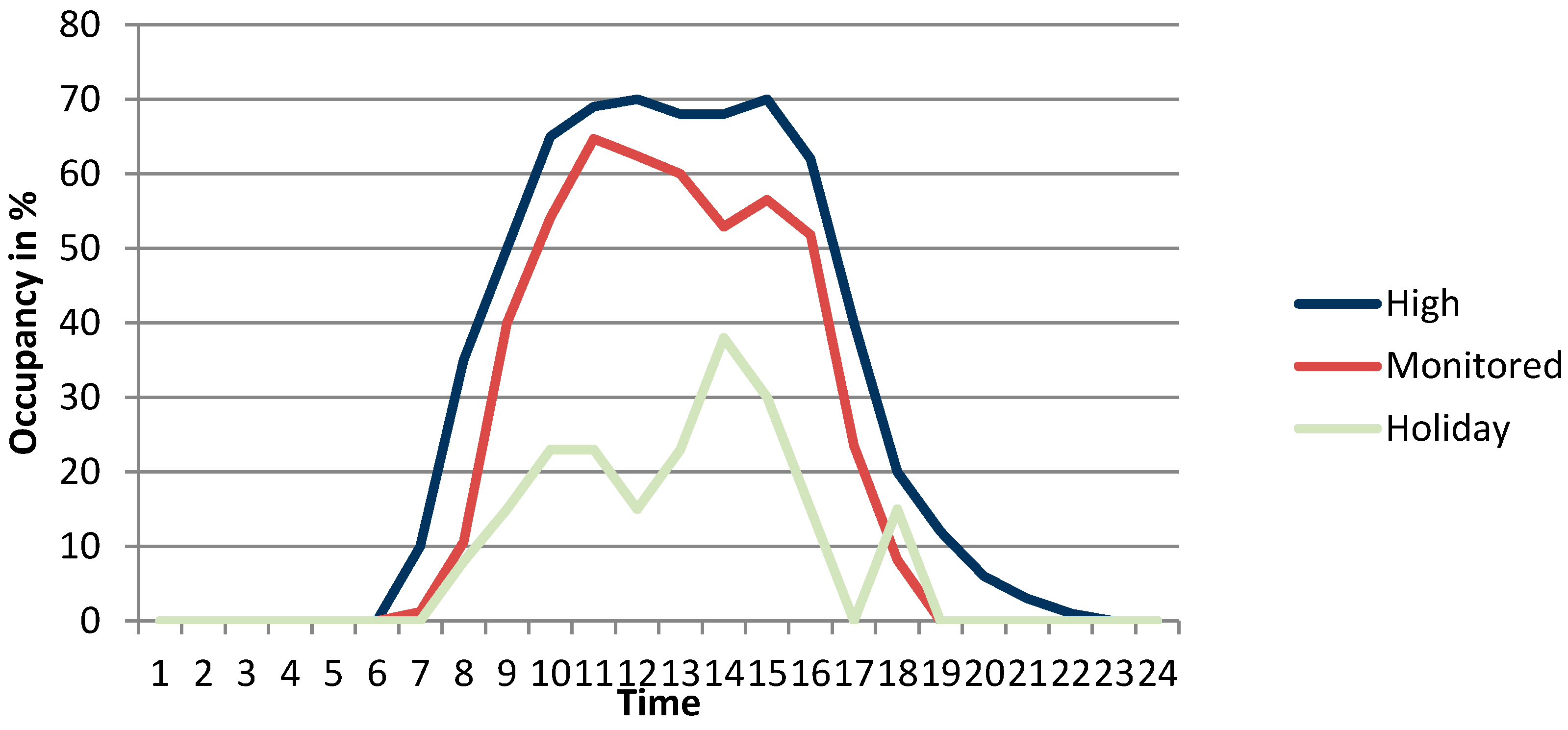
Energy simulations were carried out for a one-year period with three different scenarios for occupancy (Figure 3). The occupancy profile “Monitored” utilised an average of the results of the one week’s occupancy evaluation experiment made in case study 1. The occupancy profile “High” is a profile with higher occupancy levels and a more even curve, which was what a longer time average was supposed to look like. “Holidays” represents an estimated occupancy profile during the holiday period in July in Finland. That profile was estimated based on 25 persons’ time card presence clocking and absence information in July 2013 in a selected area of the workspaces of a Finnish research organisation.
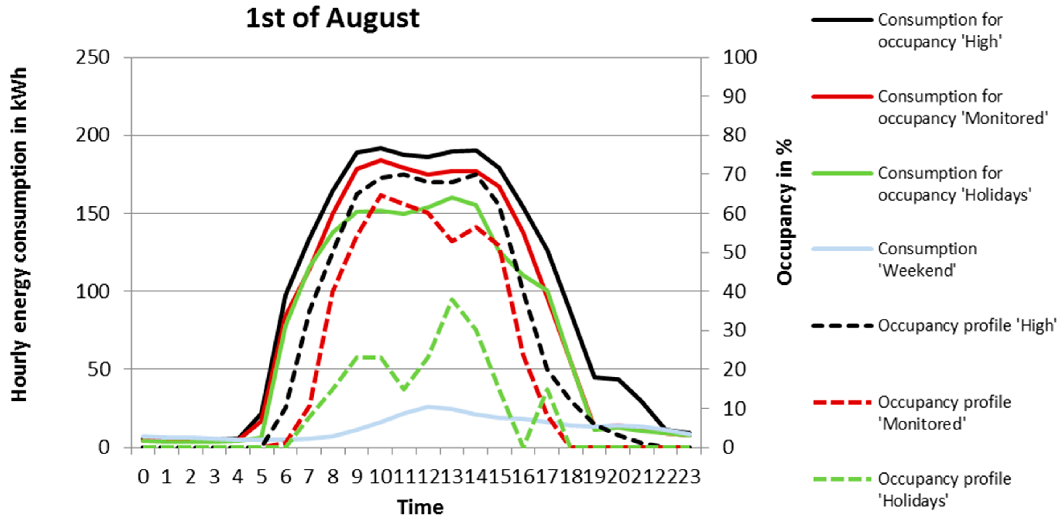
Figure 4 and Figure 5 present the results of energy simulations for two selected days: the 1st of February (in winter) and the 1st of August (in summer). These dates were chosen because, during the Finnish winter, the majority of energy is used for heating, while its consumption is low during the summer months. During summer, on the other hand, cooling and ventilation account for a big share of the energy consumption.
For winter simulations with different occupancy profiles, only a minimal difference can be observed in the energy consumption. For the summer simulations, different occupancy profiles show a difference in energy consumption, but these values are small compared to the differences in occupancy levels.
3.3. Case Study 3
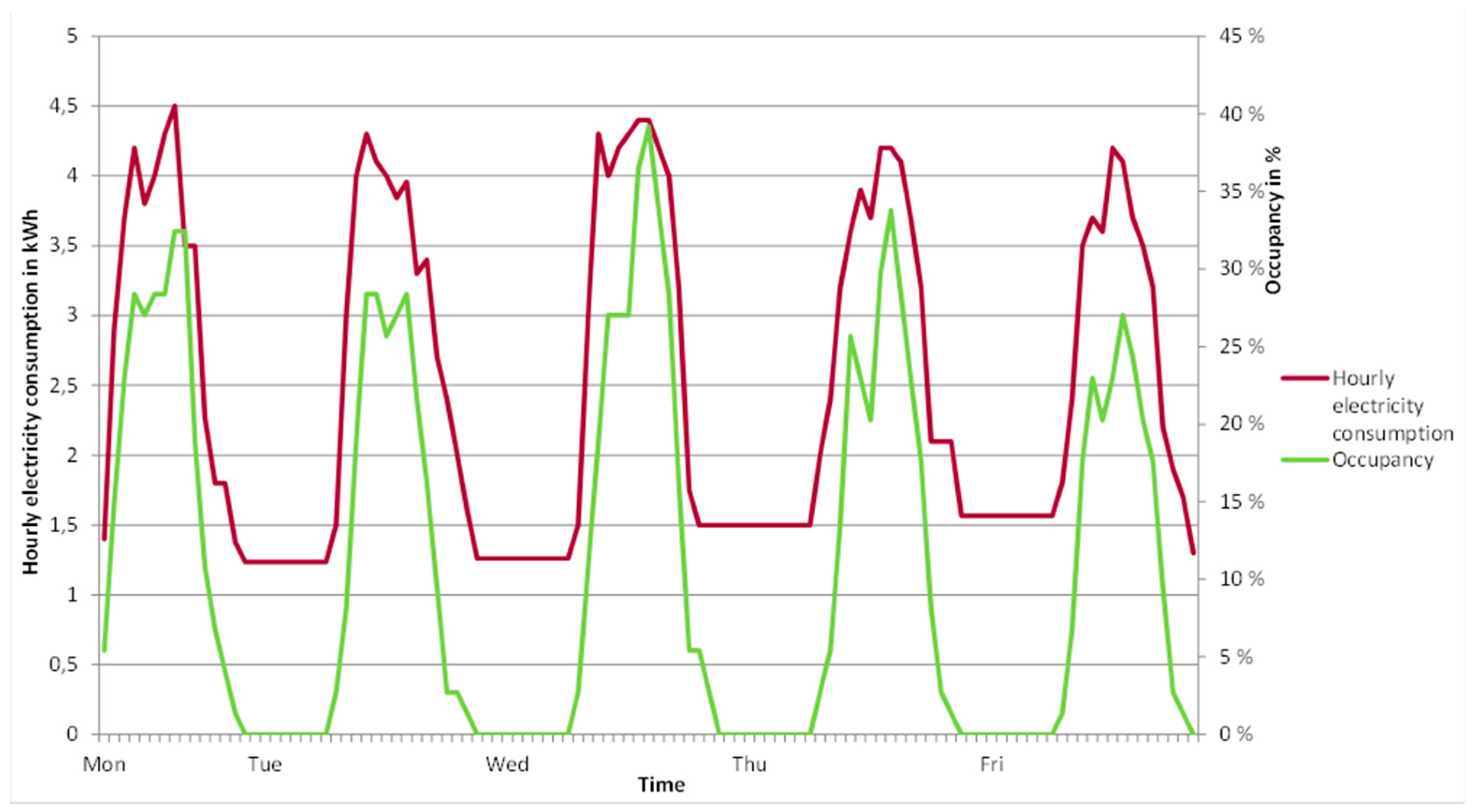
Figure 6 presents the results from monitoring the hourly occupancy levels and corresponding hourly people-related electricity consumption during one week in a workspace of a Finnish research organisation. It can be seen in the figure that the people-related electricity consumption follows the occupancy profile quite consistently. From Monday to Friday, the nightly minimum hourly electricity consumption is an average of 1.4 kWh, while the highest daily hourly consumption is an average of 4.3 kWh. The monitored electricity consumption consists of lighting, computers, and other electric devices that are plugged in. During the night time, when the building is not in use, one third of the average peak energy demand is still consumed. For occupancy levels, the daily peaks result in an average presence of 32%. The average hourly occupancy level during normal working hours (from 8 am to 4 pm) is 23%.
3.4. Case Study 4
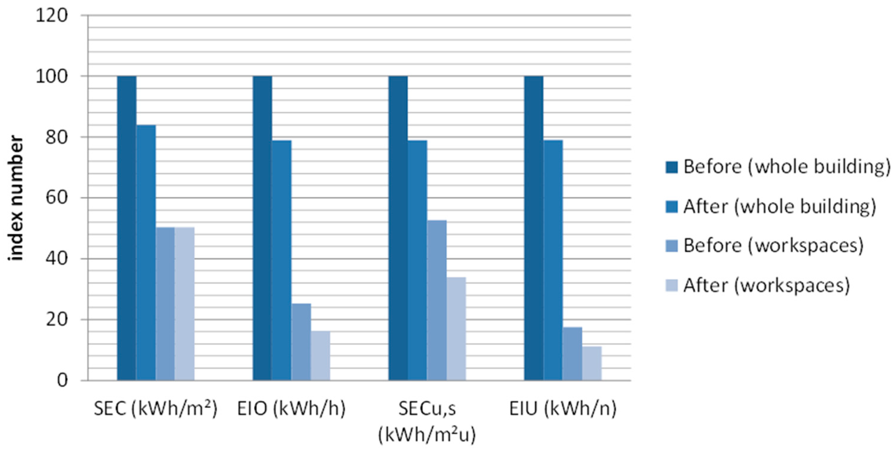
The values of the energy efficiency indicators for the various spaces have been collected in Table 5 for the situation before the renovation and in Table 6 for that after the renovation. To allow for an easier comparison of the relative differences, the values for the whole building and workspaces were indexed so that the value 100 represents the situation before the renovation in the whole building. The results of this calculation are shown in Figure 7. In general, the renovation allows a smaller energy consumption according to all of the indicators.
3.5. Case Study 5
The values of the energy efficiency indicators for the various spaces have been collected in Table 7 for the situation before the renovation and in Table 8 for that after the renovation. As opposed to the educational building in southern Finland, here we have mixed results in the sense that some indicators show lower values, and others higher values, after the renovation.
3.6. Summary of Results
Table 9 summarizes the results from the different cases. It can be clearly seen that if energy consumption is measured per floor area (SEC), a less efficient use of space is encouraged. The indicator taking into account the number of persons (EIU) is indicating well if the space is used similarly by the occupants. The indicator SECIO (kWh/m2, person hours) has the problem of overestimating the benefits of a high occupancy and/or high space efficiency. The indicator SECO has the disadvantage that it bases the calculation on relative occupancy, which is not always the optimal occupancy since the efficiency of the space layout is omitted. From the indicators, SECu,s is the only one which is able to take into account both space occupancy and space efficiency.
Based on the results of case study 2, the effect of increased occupancy levels on energy consumption is only minimal, as seen in Figure 4. Firstly, this is because it represents a winter day when heating dominates energy consumption. The amount of heating in this case is dependent on the operating times of the building and not the amount of occupants present. Moreover, there is a certain base load (see week-end consumption in Figure 4). In addition, the main heating is switched on at 6 am and switched off at 7 pm, regardless of the occupancy levels during the day. Figure 5 shows the same phenomenon from summer time and a slight effect of occupancy on energy consumption can already be seen. This is mainly due to the fact that the people-related electricity consumption is more important, since the heating loads are minimal. However, in this building, the building automation systems do not react to the actual presence of people, and in buildings which use e.g., demand-controlled ventilation, the effect of occupancy on energy consumption would naturally be more significant. Figure 6 shows that when only people-related electricity is considered (lighting, computers, and devices), the consumption follows the occupancy levels well. The base load is, however, high during night time.
In case 2, when the average daily (8 am to 4 pm) occupancy level is increased from 23% to 55%, the energy efficiency with SEC decreases by only 4%. When the average occupancy levels are increased from 55% to 65%, the effect on SEC is only 7%. Since the building in question is not intelligent, the energy consumption would be significantly more dependent on the changing operating hours of the building.
When the compared occupancy-related indicators are used, the effect is the opposite of that expected. When we consider the effect of increasing average occupancy levels by 18% (from 55% to 65%), this decreased the energy efficiency by 7% with SEC. When EIO is used, that improvement in users’ presence improves the energy efficiency by 21%, and with SECO, the improvement is 10%.
Case study 2 does not test the EIU and SECU,S indicators, since in this case, the occupancy levels are the only variable; the amount of users and space efficiency remain constant. The latter are tested with cases 4 and 5, which also show the problem with SECI,O.
Concerning the indicators of energy efficiency, Figure 7 demonstrates some of the differences that one can expect to typically appear between the figures. As the absolute values vary a lot, the indicators have been indexed so that the value before renovation for the whole building has a value of 100. From the figure, it is evident that the different indicators give quite varying results. Which indicator is the most useful depends wholly on the circumstances: what the characteristics of the building or space studied are and what purpose the results are going to be used for.
With SEC, we can see that the building consumes less energy per square meter after the renovation (case buildings 4 and 5). This shows the usefulness of the indicator when it is used to assess the technical properties of the building, regardless of its use. However, for the workspaces, no difference is expected. It has to be borne in mind that as there were no measured data from the different spaces available, the energy consumption in different spaces was estimated based on the literature. Therefore, this result is in part an artefact of the method used, while still remaining a reasonable estimate. In any case, it serves to demonstrate how even in spaces where the energy efficiency as measured by SEC is identical, the differences in the use of those spaces can produce differences in the energy efficiency when measured with another indicator. As SEC solely constitutes the amount of energy used and the floor area, it is blind to the efficiency of the use of that area.
In the case presented by Figure 7, the EIO and EIU indicators produce roughly similar results. This is because we do not expect changes in the building to produce changes in the occupancy, meaning that the same amount of personnel is expected to spend roughly the same amount of hours in the building after the renovation. They will, however, produce different results in buildings where there are changes in the usage patterns. Nonetheless, EIO and EIU have the same drawback as SEC, but in the opposite manner: they only take into account people, completely ignoring the physical area of the building.
SECU,S combines the area and occupancy into one indicator, as both are highly relevant causal factors for energy consumption in buildings. From Figure 7, it can be seen that, as one might expect, the results fall in between those from SEC and those from EIO or EIU. It produces a reasonable synthesis of the technical energy efficiency, as measured by SEC, and energy efficiency derived from the efficient use of space. By using a scalar factor u in the denominator, it produces comparable results, regardless of the size or population present in the space examined.
4. Discussion
It is evident that energy efficiency indicators play a key role when designing and operating buildings. The most common way to measure energy efficiency is to address the SEC in kWh per floor area. That indicator is very precise to measure the technical properties of a building during the design phase, but it does not perform well when the building occupancy and space efficiency are considered in the building operation phase. Basically, the more efficiently a building is used, the more energy it consumes. In general, this is seen in cases where: (1) the amount of users is increased; (2) the operating times of the building are increased; (3) its space efficiency is increased; or (4) the building users are more often present in the building. When one of these situations occurs, the building seems less energy efficient when the indicator of energy consumption per floor area is used. However, the size of the effect depends on different factors. If the building automation and control systems are not based on demand control, the effect of increased occupancy levels on energy consumption can only be minimal due to the high space heating demand, which is dependent on the operating times of the building and not the amount of occupants present.
Concerning the indicators of energy efficiency, this study demonstrates that the absolute values vary a lot, and the different indicators give quite different results. Which indicator is the most useful depends wholly on the circumstances: what the characteristics of the building or space studied are and what purpose the results are going to be used for.
Considering the SEC in [kWh/m2], it can be seen that the building consumes less energy per square meter after the energy improvements. This shows the usefulness of the indicator when it is used to assess the technical properties of the building, regardless of its use. However, for the workspaces, no difference is expected. It has to be borne in mind that as there were no measured data from the different spaces available, the energy consumption in different spaces was estimated based on the literature. Therefore, this result is in part an artefact of the method used, while still being a reasonable estimate. In any case, it serves to demonstrate how even in spaces where the energy efficiency as measured by the specific energy consumption per floor area is identical, the differences in the use of those spaces can produce differences in the energy efficiency when measured with another indicator. As the specific energy consumption per floor area solely constitutes the amount of energy used and the floor area, it is blind to the efficiency of the use of that area.
The five other indicators—EIO, EIU, SECIO, SECO, and SECU,S—were designed to take into account the efficiency of the space use. EIO and EIU are based on the amount of people, with EIU measuring the energy use per capita and EIO energy the use per person-hours, thus also covering the occupancy. In one of the cases, these two indicators produce roughly similar results. That is because we do not expect changes in the building to produce changes in the occupancy, meaning that the same amount of personnel is expected to spend roughly the same amount of hours in the building after the renovation. They will, however, produce different results in buildings where there are changes in the usage patterns. Nonetheless, EIO and EIU have the same drawback as SEC, but in the opposite manner: they only take into account people, completely ignoring the physical floor area of the building.
SECU,S was devised here to combine the area and occupancy into one indicator, as both are highly relevant causal factors for energy consumption in buildings. This indicator produces a reasonable synthesis of the technical energy efficiency, as measured by SEC, and energy efficiency derived from efficient use of space.
5. Conclusions
This study clearly showed that energy efficiency can be measured by using different indicators and it also confirmed that different indicators have different impacts on the results showing the efficiency. Traditionally, the energy efficiency in a building has been measured by using the specific energy consumption, SEC, in units of kWh/m2. That indicator is very useful for the design phase, when the actual amount of occupants is only an estimate. That indicator is very useful for comparing technical solutions in the building design phase. It is easy to calculate and there are plenty of documented cases based on this indicator.
The indicator corresponding to the amount of persons in the building, illustrating the energy intensity of usage, EIU, kWh/person, is illustrative when space efficiency is considered and when the space of the building is fixed. That is typically the case in existing buildings or in dwellings. The advantage of this indicator is that it is very easy to calculate.
The indicator of energy intensity of occupancy (EIO), kWh/person hours, is a good indicator of the space efficiency and occupancy, but it has the disadvantage that, as with EIU, it omits the size of the building and therefore is not appropriate to compare the technical aspects of energy efficiency.
The indicator SECIO in unit of kWh/m2, person hours, has the advantage that it takes into account both the space use, but also the amount of persons using the space. However, the problem in using this indicator is that it overestimates the effect of the space and person hour efficiency in an exponential way.
The indicator of SEC adjusted for occupancy, SECO, highlights the relative occupancy. This indicator does not take into account the space efficiency. The handicap in this indicator is that even 100% occupancy is not optimal in some cases.
The SEC adjusted for occupancy and space efficiency, SECU,S, is the only indicator taking both relevant aspects into account. Currently, this indicator is rather difficult to calculate in real buildings since the data for accurate real time occupancy is not easily available. However, in the future, when more sensors are installed and when the internet of things can make information flow easier, the calculation of SECU,R will be easier. Once cheap and reliable people tracking methods are available, the use of this indicator can be upscaled to a district or city scale, which will offer huge energy and emission saving potential since the local energy system can be better optimized based on demand and the different use patterns in different building typologies (e.g., residential and offices).
It is very important to develop tools to collect real time data of both energy and occupancy, since building users are very often encouraged to save energy based on measured energy consumption. Thus, it is critical to know that the indicator used to assess the energy efficiency is truly guiding the building use towards one which is sustainable.
Acknowledgments
This study was part of VTT Innovation program Ingrid, Intelligent energy networks, and smart districts. This study was funded by the Academy of Finland, Strategic Research Council, the Finnish Funding Agency for Innovation Tekes and the RYM Ltd. PRE program NewWoW. Smart Energy Transition project (293405) thanks the Strategic Research Council in collaboration with the Academy of Finland for their continuing support for the project. The funding sources are greatly acknowledged. In addition, acknowledgements are due to Anni Tyni for support in the energy simulations of case study 2, Granlund Oy for participating in case study 1 experiments and Rapal Oy for providing equipment used in case study 1.
Author Contributions
Aapo Huovila conceived, designed and performed the experiments, analysed the data and wrote the chapters related to case studies 1, 2 and 3. Pekka Tuominen did the calculations and analysed the results for case studies 4 and 5. Miimu Airaksinen was responsible for designing and carrying on the case studies 4 and 5, in addition she was responsible of the design of the article. All the authors designed together the new suggested indicators presented in 2.1 and wrote the chapters 1, 2.1, 3.6, 4 and 5.
Conflicts of Interest
The authors declare no conflict of interest.
References
- Laustsen, J. Energy Efficiency Requirements in Building Codes, Energy Efficiency Policies for New Buildings; International Energy Agency: Paris, France, 2008. [Google Scholar]
- IEA. Worldwide Trends in Energy Use and Efficiency; International Energy Agency: Paris, France, 2008. [Google Scholar]
- IPCC. Summary for Policymakers—Contribution of Working Group III to the Fourth Assessment Report of the Intergovernmental Panel on Climate Change; Cambridge University Press: Cambridge, UK, 2007. [Google Scholar]
- Action Plan for Energy Efficiency: Realising the Potential, COM(2006)545; European Commission: Brussels, Belgium, 2006.
- Efficiency in Buildings—Transforming the Market; World Business Council for Sustainable Development: Geneva, Switzerland, 2009.
- Belzer, D.B. Energy Efficiency Potential in Existing Commercial Buildings; Pacific Northwest National Laboratory: Richland, WA, USA, 2009.
- Dooley, K. New ways of working: Linking energy consumption to people. In Proceedings of the SB11 Helsinki World Sustainable Building Conference, Helsinki, Finland, 18–21 October 2011. [Google Scholar]
- Martani, C.; Lee, D.; Robinson, P.; Britter, R.; Ratti, C. ENERNET: Studying the dynamic relationship between building occupancy and energy consumption. Energy Build. 2012, 47, 584–591. [Google Scholar] [CrossRef]
- Mendes, G.; Feng, W.; Stadler, M.; Steinbach, J.; Lai, J.; Zhou, N.; Marnay, C.; Ding, Y.; Zhao, J.; Tian, Z.; et al. Regional analysis of building distributed energy costs and CO2 abatement: A U.S.–China comparison. Energy Build. 2014, 77, 112–129. [Google Scholar]
- Chung, W.; Hui, Y.V. A study of energy efficiency of private office buildings in Hong Kong. Energy Build. 2009, 41, 696–701. [Google Scholar]
- Pikas, E.; Thalfeldt, M.; Kurnitski, J. Cost optimal and nearly zero energy building solutions for office buildings. Energy Build. 2014, 74, 30–42. [Google Scholar] [CrossRef]
- Zhao, J.; Wu, Y.; Zhu, N. Implementing effect of energy efficiency supervision system for government office buildings and large-scale public buildings in China. Energy Policy 2009, 37, 2079–2086. [Google Scholar] [CrossRef]
- Boyano, A.; Hernandez, P.; Wolf, O. Energy demands and potential savings in European office buildings: Case studies based on EnergyPlus simulations. Energy Build. 2013, 65, 19–28. [Google Scholar] [CrossRef]
- Nunes, P.; Lerer, M.; Carrilho da Graça, G. Energy certification of existing office buildings: Analysis of two case studies and qualitative reflection. Sustain. Cities Soc. 2013, 9, 81–95. [Google Scholar] [CrossRef]
- Sustainable Energy Authority of Ireland (SEAI). Methodology for the Production of Display Energy Certificates (DEC); SEAI: Dublin, Ireland, 2013. [Google Scholar]
- Better Buildings Partnership (BBP). Sustainability Benchmarking Toolkit for Commercial Buildings. Principles for Best Practice; BBP: London, UK, 2010. [Google Scholar]
- Bordass, B. Notes on Benchmarking Building Energy Performance for Occupation Density; The Usable Buildings Trust: London, UK, 2011. [Google Scholar]
- IPD. Occupancy Density, Energy Consumption and Carbon Emissions in Central Government Offices. Phase 1 Report. 2010. Available online: http://www.sballiance.org/wp-content/uploads/2014/04/IPD-Environment-Code-2010.pdf (accessed on 2 May 2017).
- Forsström, J.; Lahti, P.; Pursiheimo, E.; Rämä, M.; Shemeikka, J.; Sipilä, K.; Tuominen, P.; Wahlgren, I. Measuring Energy Efficiency. Indicators and Potentials in Buildings, Communities and Energy Systems, VTT Research Notes 2581; VTT Technical Research Centre of Finland: Espoo, Finland, 2011. [Google Scholar]
- Huovila, A.; Tyni, A.; Dooley, K. Building occupancy as an aspect of energy efficiency. In Proceedings of the SB13 Conference, Dubai, UAE, 8–10 December 2013. [Google Scholar]
- D’Oca, S.; Hong, T. Occupancy schedules learning process through a data mining framework. Energy Build. 2015, 88, 395–408. [Google Scholar] [CrossRef]
- Duarte, C.; Van Den Wymelenberg, K.; Rieger, C. Revealing occupancy patterns in an office building through the use of occupancy sensor data. Energy Build. 2013, 67, 587–595. [Google Scholar] [CrossRef]
- Van Dronkelaar, C.; Dowson, M.; Burman, E.; Spataru, C.; Mumovic, D. A review of the energy performance gap and its underlying causes in non-domestic buildings. Front. Mech. Eng. 2016, 1, 17. [Google Scholar] [CrossRef]
- Karjalainen, S. Should we design buildings that are less sensitive to occupant behaviour? A simulation study of effects of behaviour and design on office energy consumption. Energy Effic. 2016, 9, 1257–1270. [Google Scholar]
- Erickson, V.L.; Carreira-Perpiñán, M.Á.; Cerpa, A.E. Occupancy modeling and prediction for building energy management. ACM Trans. Sens. Netw. 2014, 10, 42. [Google Scholar] [CrossRef]
- Taylor, C.E. Occupancy matching. Energy Eng. 2015, 112, 11–21. [Google Scholar]
- Labeodan, T.; Zeiler, W.; Boxem, G.; Zhao, Y. Occupancy measurement in commercial office buildings for demand-driven control applications—A survey and detection system evaluation. Energy Build. 2015, 93, 303–314. [Google Scholar] [CrossRef]
- Hietanen, P. Paljonko Tilaa Organisaatio Tarvitsee? Työympäristökehittämisen Ympäristövaikutukset. KIINKO KIPA Project Work, Senate Properties. 2009, p. 33. Available online: https://www.slideshare.net/paihiet/paljonko-tilaa-organisaatio-tarvitsee-tyoymparistokehittamisen-ymparistovaikutukset-pivi-hietanen-2009 (accessed on 4 May 2017). (In Finnish).
- Finnish Ministry of Finance. Valtion toimitilastrategia (State Strategy for Premises). 16 November 2005. Available online: http://vm.fi/documents/10623/307565/Toimitilastrategia+2020/964fa234-3698-4b74-aadf-5c15aa6cdb4d (accessed on 2 May 2017). (In Finnish).
- Rapal. Optimaze.net Active Space Optimization Tool. Available online: http://rapal.com/optimaze/space-utilization-studies-made-easy/ (accessed on 2 May 2017).
- Rinne, S. HINKU-kuntien rakennusten energiankäytön tehostamis- ja säästöselvitys; Enespa Oy: Helsinki, Finland, 2009. [Google Scholar]
- McCann, A. Energy Efficiency in Laboratory Buildings; University of Strathclyde: Glasgow, UK, 2007. [Google Scholar]
- IDA Simulation Environment. Available online: http://www.equa-solutions.co.uk/ (accessed on 31 October 2012).
- Sahlin, P.; Eriksson, L.; Grozman, P.; Johnsson, H.; Shapovalov, A.; Vuolle, M. Whole-building simulation with symbolic DAE equations and general purpose solvers. Build. Environ. 2012, 39, 949–958. [Google Scholar] [CrossRef]
- Sahlin, P.; Eriksson, L.; Grozman, P.; Johnsson, H.; Shapovalov, A.; Vuolle, M. Will equation-based building simulation make it? Experiences from the introduction of IDA indoor climate and energy. In Proceedings of the 8th International (IBPSA) International Building Performance Simulation Association Conference, Eindhoven, The Netherlands, 11–14 August 2003. [Google Scholar]
Figure 1.
Occupancy levels obtained with different methods; example of one workday.
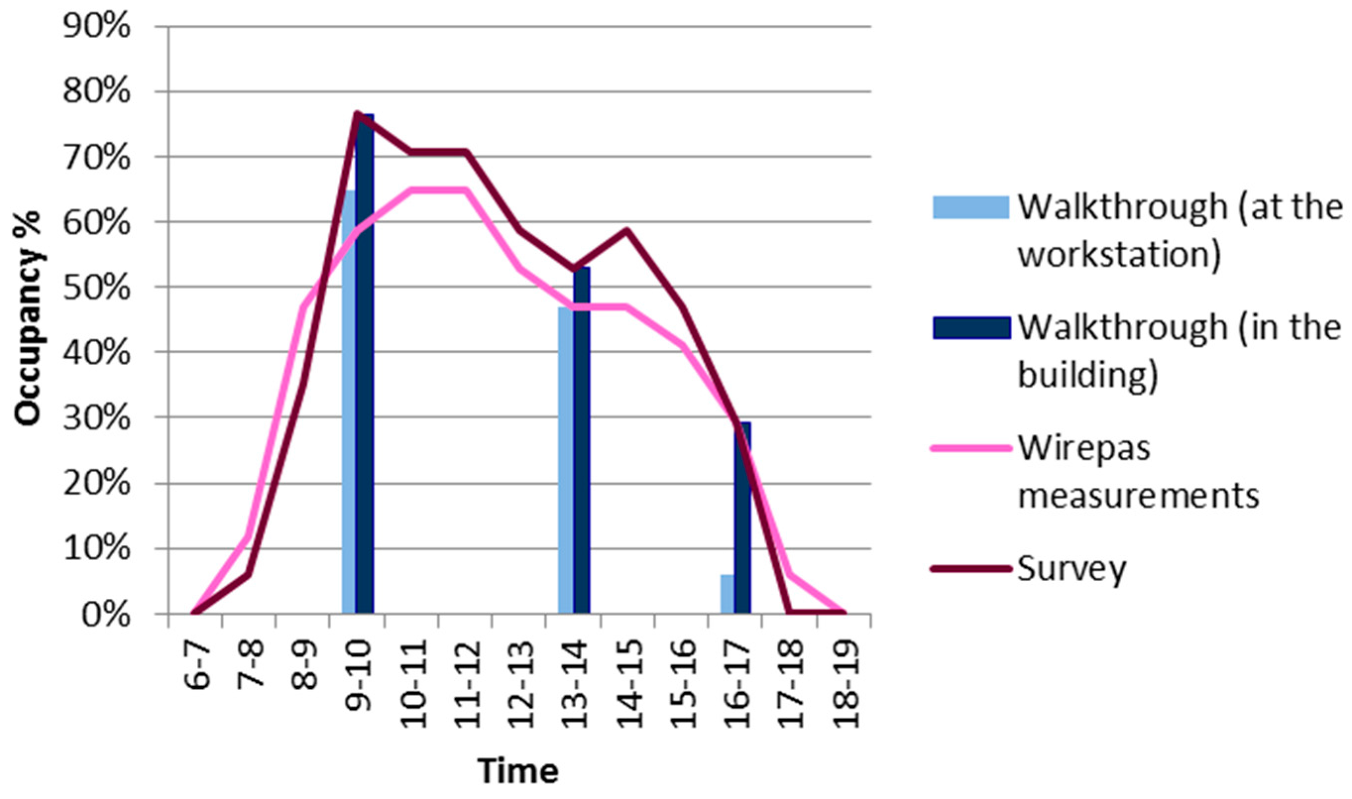
Figure 2.
Results from the occupancy measurements with Wirepas. The lower horizontal line shows the seats required and the upper horizontal line represents the seats available.
Figure 2.
Results from the occupancy measurements with Wirepas. The lower horizontal line shows the seats required and the upper horizontal line represents the seats available.
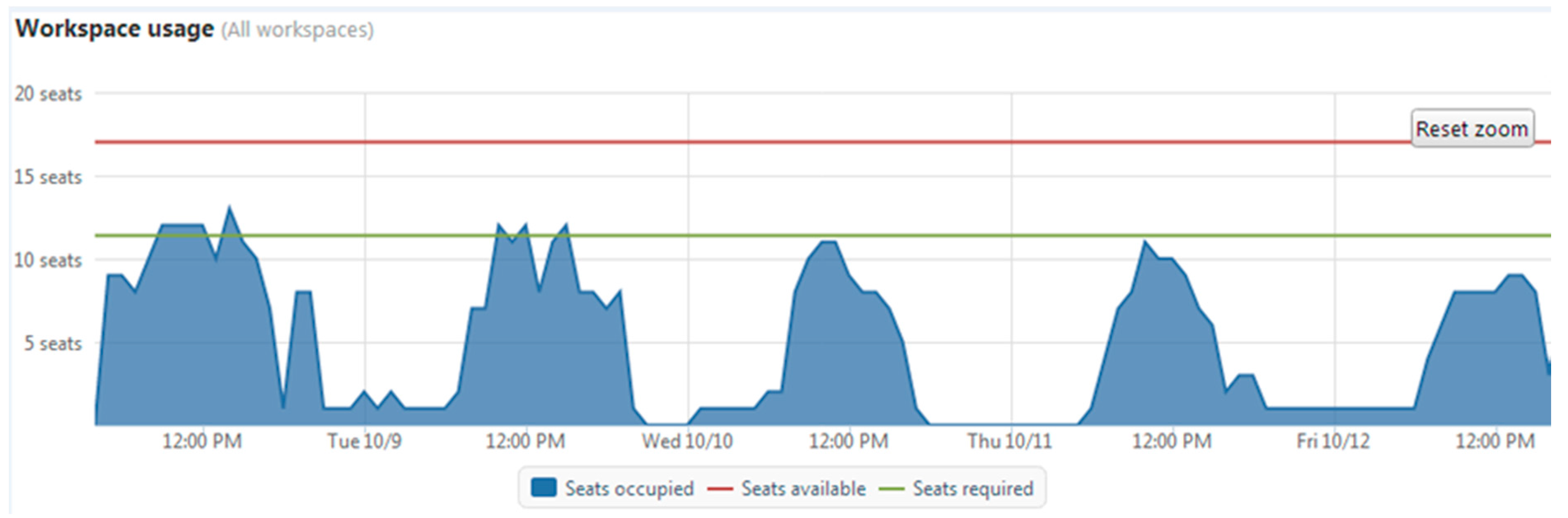
Figure 3.
Occupancy profiles used in dynamic energy simulations.

Figure 4.
Energy simulations for 1st of February (winter) with different occupancy profiles.
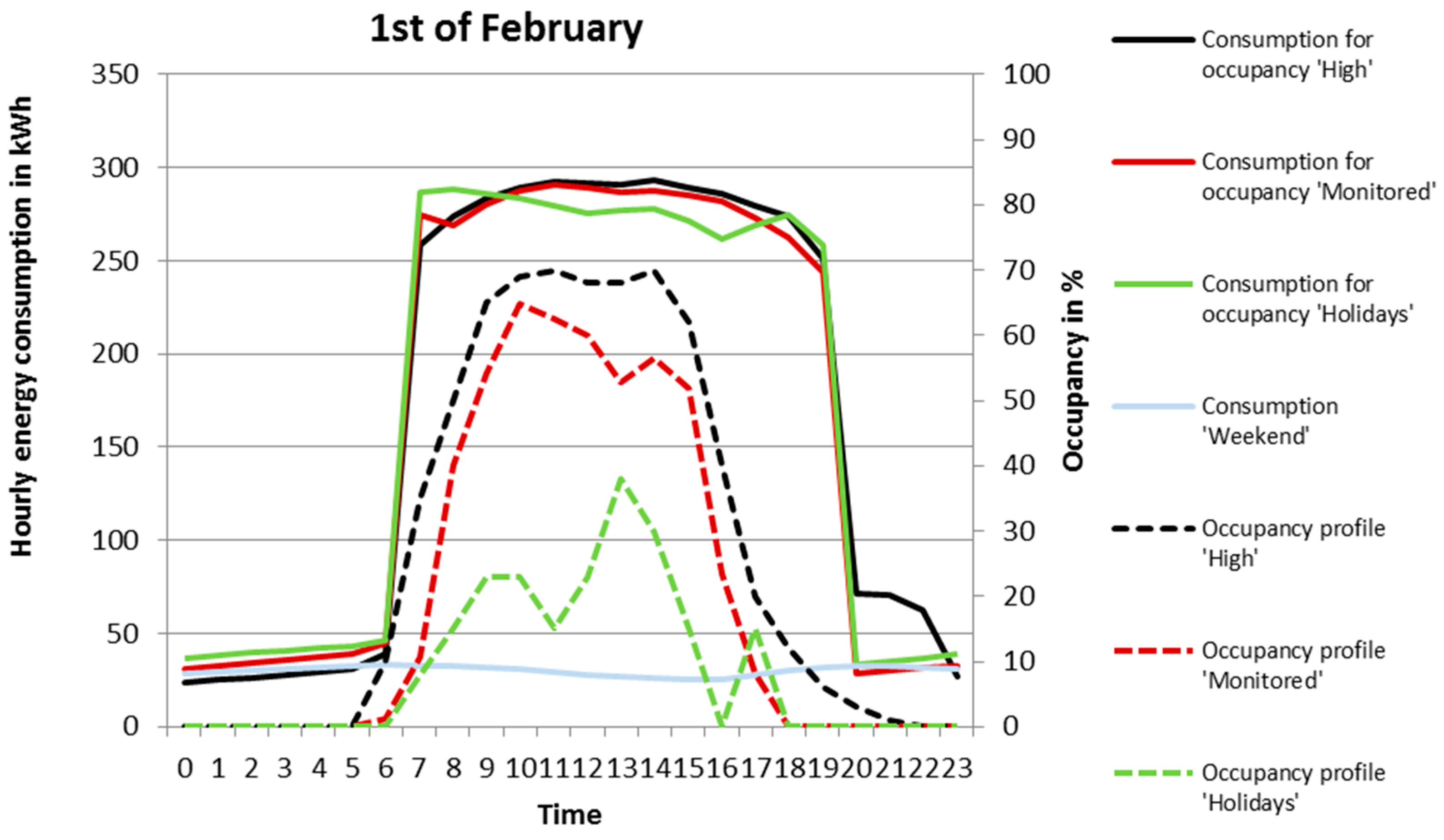
Figure 5.
Energy simulations 1st of August (summer) with different occupancy profiles.

Figure 6.
Effect of occupancy on people-related electricity consumption based on monitoring.

Figure 7.
Indexed values (100 = whole building before the renovation) for energy efficiency indicators for the whole building and the workspaces.
Figure 7.
Indexed values (100 = whole building before the renovation) for energy efficiency indicators for the whole building and the workspaces.


Table 1.
Indicators used in this study. SEC: specific energy consumption; EIU: energy intensity of usage; EIO: energy intensity of occupancy; SECIO: SEC per intensity of occupancy; SECO: SEC adjusted for occupancy; SECu,s: specific energy consumption adjusted for occupancy and space efficiency.
Table 1.
Indicators used in this study. SEC: specific energy consumption; EIU: energy intensity of usage; EIO: energy intensity of occupancy; SECIO: SEC per intensity of occupancy; SECO: SEC adjusted for occupancy; SECu,s: specific energy consumption adjusted for occupancy and space efficiency.
| Indicator Name | Unit | Reference |
|---|---|---|
| SEC | kWh/m2. | The traditional indicator for energy efficiency used in most existing studies, e.g., [9,10,11,12,13,14] |
| EIU | kWh/nperson, nperson = number of occupants. | [7,18,19,20] |
| EIO | kWh/hpers, hpers = sum of the number of hours that each building occupant spends in the building during the year in question. | Similar indicators presented in [17,19] |
| SECIO | kWh/m2, hpers, hpers = sum of the number of hours that each building occupant spends in the building during the year in question. | Similar indicators presented in [7,20] |
| SECO | kWh/m2o, o = average presence of the occupants during normal working hours 8–17 and normal workdays. 0 ≤ o ≤ 1. | Similar indicators presented in [19,20] |
| SECu,s | kWh/m2u, u = (ntavg)/(A/aref *tref), where n is the actual number of people using the space, tavg is the average number of hours present daily per person, A is the total area studied. The parameters aref and tref are normalising factors: aref is the amount of space per person available in a typical office setting and tref represent normal working hours, in this paper we use the value 8 h. For aref typical figures from Finland was used: 12 m2/person when only workspace is considered and 25 m2/person [29] when the whole office building is considered. | New indicator proposed by this paper |
Table 2.
The main functions of the building and their floor areas and person hours in the original plan and in the plan after renovation.
Table 2.
The main functions of the building and their floor areas and person hours in the original plan and in the plan after renovation.
| Original | After Renovation | ||||||
|---|---|---|---|---|---|---|---|
| Space Types | Number of Persons | Person Hours | Gross Floor Area (m²) | Space Types | Number of Persons | Person Hours | Gross Floor Area (m²) |
| Workspaces | 97 | 2484 | 2468 | Workspaces | 121 | 3105 | 1984 |
| Large teaching spaces | 49 | 213 | 842 | Teaching spaces | 125 | 464 | 1486 |
| Small teaching spaces | 51 | 158 | 77 | ||||
| Laboratories | 50 | 503 | 2583 | Laboratories | 63 | 629 | 1952 |
| Meeting rooms | 4 | 126 | 540 | Multipurpose spaces | 5 | 158 | 2107 |
| Coffee room | 39 | 81 | 119 | Common areas | 49 | 101 | 367 |
| Library | 16 | 6149 | 944 | Library | |||
| Computer classes | 13 | 29 | 467 | Computer classes | 16 | 36 | 448 |
| Passageways and toilets | 97 | 315 | 3155 | Passageways and toilets | 125 | 379 | 3036 |
| Storage and technical spaces | 97 | 0 | 1733 | Storage and technical spaces | 121 | 0 | 1551 |
Table 3.
The main functions of the building and the floor areas and person hours in original plan and in the plan after renovation.
Table 3.
The main functions of the building and the floor areas and person hours in original plan and in the plan after renovation.
| Original | After Renovation | ||||||
|---|---|---|---|---|---|---|---|
| Space Types | Number of Persons | Person Hours | Gross Floor Area (m²) | Space Types | Number of Persons | Person Hours | Gross Floor Area (m²) |
| Archives | 9 | 23 | 337 | Archives | 9 | 23 | 337 |
| Workspaces | 54 | 2321 | 1854 | Workspaces | 54 | 2321 | 1854 |
| Customer areas | 13 | 104 | 84 | Customer areas | 13 | 104 | 84 |
| Meeting rooms | 174 | 174 | 203 | Meeting rooms | 174 | 174 | 203 |
| Educational spaces | 28 | 96 | 85 | Educational spaces | 28 | 96 | 85 |
| Break rooms | 10 | 34 | 162 | Break rooms | 10 | 34 | 162 |
| Other spaces | 4 | 49 | 816 | Other spaces | 4 | 49 | 816 |
Table 4.
Average energy consumption values in various spaces in Finland (kWh/m²/a) according to [31].
Table 4.
Average energy consumption values in various spaces in Finland (kWh/m²/a) according to [31].
| Space Type | Heat | Electricity |
|---|---|---|
| Gathering | 225 | 107 |
| Storage | 242 | 65 |
| Educational | 203 | 55 |
| Office | 170 | 68 |
Table 5.
Values of energy efficiency indicators for the various spaces before the renovation.
| Space Types | kWh/m² | kWh/hpersons | kWh/m²u | kWh/npersons |
|---|---|---|---|---|
| Whole building | 545 | 20.6 | 1358 | 39,849 |
| Workspaces | 274 | 5.2 | 907 | 6965 |
| Large teaching spaces | 303 | 23.0 | 5214 | |
| Small teaching spaces | 362 | 3.4 | 547 | |
| Laboratories | 982 | 96.6 | 50,746 | |
| Meeting rooms | 382 | 31.3 | 51,511 | |
| Library | 274 | 0.8 | 16,144 | |
| Computer classes | 267 | 82.4 | 9597 | |
| Passageways and toilets | 274 | 52.4 | 8902 |
Table 6.
Values of energy efficiency indicators for the various spaces after the renovation.
| Space Types | SEC (kWh/m²) | EIO (kWh/hpersons) | SECu,s (kWh/m²u) | EIU (kWh/npersons) |
|---|---|---|---|---|
| Whole building | 457 | 16.3 | 1721 | 31,514 |
| Workspaces | 274 | 3.4 | 583 | 4478 |
| Teaching spaces | 303 | 18.6 | 3606 | |
| Laboratories | 982 | 58.4 | 30,676 | |
| Multipurpose spaces | 316 | 80.9 | 133,000 | |
| Common areas | 321 | 22.3 | 2414 | |
| Computer classes | 267 | 63.2 | 7359 | |
| Passageways and toilets | 274 | 41.9 | 6647 |
Table 7.
Values of energy efficiency indicators for the various spaces before the renovation.
| Space Types | SEC (kWh/m²) | EIO (kWh/hpersons) | SECu,s (kWh/m²u) | EIU (kWh/npersons) |
|---|---|---|---|---|
| Whole building | 192 | 4.6 | 388 | 3905 |
| Workspaces | 190 | 2.9 | 506 | 6526 |
| Customer areas | 190 | 2.9 | - | 1225 |
| Meeting rooms | 190 | 4.2 | - | 222 |
| Educational spaces | 194 | 3.3 | - | 591 |
| Break rooms | 207 | 19.0 | - | 3366 |
| Other spaces | 177 | 56.5 | - | 36,128 |
| Archives | 231 | 64.9 | - | 8655 |
Table 8.
Values of energy efficiency indicators for the various spaces after the renovation.
| Space Types | SEC (kWh/m²) | EIO (kWh/hpersons) | SECu,s (kWh/m²u) | EIU (kWh/npersons) |
|---|---|---|---|---|
| Whole building | 263 | 2.7 | 228 | 2345 |
| Workspaces | 262 | 1.7 | 299 | 3859 |
| Customer areas | 262 | 1.7 | - | 724 |
| Meeting rooms | 262 | 2.5 | - | 131 |
| Educational spaces | 263 | 1.9 | - | 343 |
| Break rooms | 281 | 11.0 | - | 1956 |
| Other spaces | 242 | 33.1 | - | 21,186 |
| Archives | 313 | 37.6 | - | 5019 |
Table 9.
Summary of the different indicators in the studied cases.
| Case Study | Area, m2 | Number of Occupants | m2/Person | Method for Estimating Occupancy | u as Defined in Table 1 | o as Defined in Table 1 (Average Occupancy during Office Hours 8–17) | Average Person Hours per Person per Year (Extrapolated for 261 Yearly Workdays) | Method to Evaluate Energy Consumption, Coverage | SEC (kWh/m2) | EIU (kWh/Person) | EIO (kWh/Person Hours) | SECIO kWh/m2, Person Hours | SECO kWh/(o*m2) | SECus kWh/(u*m2) |
|---|---|---|---|---|---|---|---|---|---|---|---|---|---|---|
| 2 (high occupancy) | 4123 | 310 | 13.3 | Hypothetical “high” | 1.52 | 62% | 1691 | Simulation | 136 | 1808 | 1.07 | 0.00026 | 219 | 89.5 |
| 2 (real occupancy measured in case study 1) | 4123 | 310 | 13.3 | Measured in case study 1 | 1.13 | 52% | 1253 | Simulation | 127 | 1686 | 1.35 | 0.00033 | 244 | 112.2 |
| 2 (low holiday occupancy) | 4123 | 310 | 13.3 | Estimated “holiday” | 0.51 | 20% | 564 | Simulation | 122 | 1623 | 2.88 | 0.0007 | 610 | 239.1 |
| 3 | 367.2 | 37 | 9.9 | Real, manually hourly | 0.35 | 27% | 598 | Hourly measured, only people related electricity for 7 days; annual extrapolated by multiplying by 52.14 | 50 | 492 | 0.82 | 0.0023 | 183 | 141.6 |
| 4 (before renovation) | 3541 | 174 | 20.4 | Questionnaire | 0.49 | 66% | 1550 | Measured | 192 | 3905 | 4.6 | 0.0013 | 291 | 388 |
| 4 (after renovation) | 1550 | 174 | 8.9 | Questionnaire | 1.15 | 66% | 1550 | Measured | 263 | 2345 | 2.7 | 0.0017 | 398 | 228 |
| 5 (before renovation) | 8549 | 97 | 88.1 | Questionnaire | 0.32 | 77% | 1809 | Measured | 545 | 39,849 | 20.6 | 0.0024 | 708 | 1721 |
| 5 (after renovation) | 9526 | 121 | 78.7 | Questionnaire | 0.34 | 77% | 1809 | Measured | 457 | 31,514 | 16.3 | 0.0017 | 594 | 1358 |
| 5 (workstations before renovation) | 2468 | 97 | 25.4 | Questionnaire | 0.30 | 53% | 1245 | Measured, distributed based on literature | 274 | 6965 | 5.2 | 0.0021 | 517 | 907 |
| 5 (workstations after renovation) | 1984 | 121 | 16.4 | Questionnaire | 0.47 | 53% | 1245 | Measured, distributed based on literature | 274 | 4478 | 3.4 | 0.0017 | 517 | 583 |
© 2017 by the authors. Licensee MDPI, Basel, Switzerland. This article is an open access article distributed under the terms and conditions of the Creative Commons Attribution (CC BY) license (http://creativecommons.org/licenses/by/4.0/).
Share and Cite
MDPI and ACS Style
Huovila, A.; Tuominen, P.; Airaksinen, M. Effects of Building Occupancy on Indicators of Energy Efficiency. Energies 2017, 10, 628. https://doi.org/10.3390/en10050628
AMA Style
Huovila A, Tuominen P, Airaksinen M. Effects of Building Occupancy on Indicators of Energy Efficiency. Energies. 2017; 10(5):628. https://doi.org/10.3390/en10050628
Chicago/Turabian StyleHuovila, Aapo, Pekka Tuominen, and Miimu Airaksinen. 2017. "Effects of Building Occupancy on Indicators of Energy Efficiency" Energies 10, no. 5: 628. https://doi.org/10.3390/en10050628
Note that from the first issue of 2016, this journal uses article numbers instead of page numbers. See further details here.