
Case Study on the Socio-Economic Benefit of Allowing Active Power Curtailment to Postpone Grid Upgrades

1
SINTEF Energy Research, NO-7465 Trondheim, Norway
2
Agder Energi Nett AS, NO-4848 Arendal, Norway
*
Author to whom correspondence should be addressed.
Energies 2017, 10(5), 632; https://doi.org/10.3390/en10050632
Submission received: 22 December 2016
/
Revised: 22 March 2017
/
Accepted: 28 April 2017
/
Published: 5 May 2017
(This article belongs to the Special Issue Sustainable and Renewable Energy Systems)
Abstract
:The penetration of distributed generation is rapidly increasing in the power system. Traditionally, a fit-and-forget approach has been applied for grid integration of distributed generation, by investing in a grid capacity that can deal with worst-case situations. However, there is now increasing interest for the possible cost savings that can be achieved through more active network management. This paper presents a case study on the possible socio-economic benefit of postponing a grid upgrade in an area of surplus generation. Two alternatives for grid integration of an 8 MW run-on-river hydro power plant in the southern part of Norway are investigated: (i) grid upgrade; and (ii) active power curtailment whenever needed to avoid network congestion. This study shows that cost savings corresponding to 13% of the investment cost for the grid upgrade is possible through active power curtailment.
1. Introduction
The number of distributed generation units in the power system is rapidly increasing worldwide, and integration of distributed generation based on renewable resources is an important measure in order to meet the world’s increasing energy demand in a sustainable way [1]. However, integration of a large amount of variable production from renewable sources may impose challenges to the distribution grid, such as violation of voltage or current limits [2,3]. Traditionally, a fit-and-forget approach has been applied when integrating distributed generation to the power system. Consequently, the grid has to be designed for the worst case, typically being minimum load and maximum generation, even if these conditions only occur for a few hours each year. This conservative approach may prevent integration of renewable distributed generation due to high costs related to grid upgrades.
There has been extensive research on alternative measures of increasing the grids’ hosting capacity for distributed generation in the past few decades, and there seems to be a consensus that a transition to a more active distribution network management would be favorable [4,5,6,7].
Several different methods related to increasing the hosting capacity with the use of active network management strategies are proposed in the literature, including coordinated voltage control and reactive power compensation [8,9,10,11], active power curtailment [12,13,14], or a combination of the two [6,15,16,17,18,19]. Several countries (not including Norway) allow the utilization of active power curtailment as an alternative to grid investments, and thus allow grid companies to plan for curtailment of generation and delay/avoid reinforcement for practical or economic reasons [3]. Methods for optimizing the operation of active networks are also discussed in the literature [19,20,21]. There is a balance between minimizing the costs of energy curtailment and the cost of transmission losses.
Active network management strategies in order to increase the hosting capacity in a grid will typically result in higher transmission losses compared to the traditional method of upgrading the grid. This will limit how much the hosting capacity can be increased through active management strategies before grid upgrades become the preferred solution. In [22], a method for finding the optimal hosting capacity with the use of active network management strategies, considering grid reinforcement cost, cost of transmission losses, and energy curtailment costs, as seen from both the distribution system operator (DSO) and the wind farm operator is suggested. There are also other studies that consider economic aspects of active network management compared with grid upgrades [12,23,24]. However, there are few studies focused on the potential socio-economic benefits of utilizing active power curtailment to postpone grid investments.
This paper presents a case study on the socio-economic gains of allowing active power curtailment as an alternative to grid upgrade for a specific case of relevance for a grid company in Southern Norway. The paper will also present a method for comparing these two alternatives for increasing the hosting capacity of the grid.
2. Case Description
In 2007, an 8 MW run-on-river hydro power plant was connected to a regional grid within a surplus area in Sothern Norway. As a result, the total surplus within the area could exceed the grid capacity in some hours during the year if no actions were taken. The capacity of the existing connection out of the area was 29 MW, while Table 1 shows that the required capacity after connection of the new generation will be 32 MW. The values in Table 1 are based on measurements of the maximum power injection from new and existing generation and the minimum load, and the calculated losses for this situation. In this study, it is a premise that the capacity in the overlying transmission grid is sufficient to handle the generation from the new run-on-river hydro power plant without any power rejections [25]. The two considered measures are described below.
2.1. Alternative 1: Active Power Curtailment
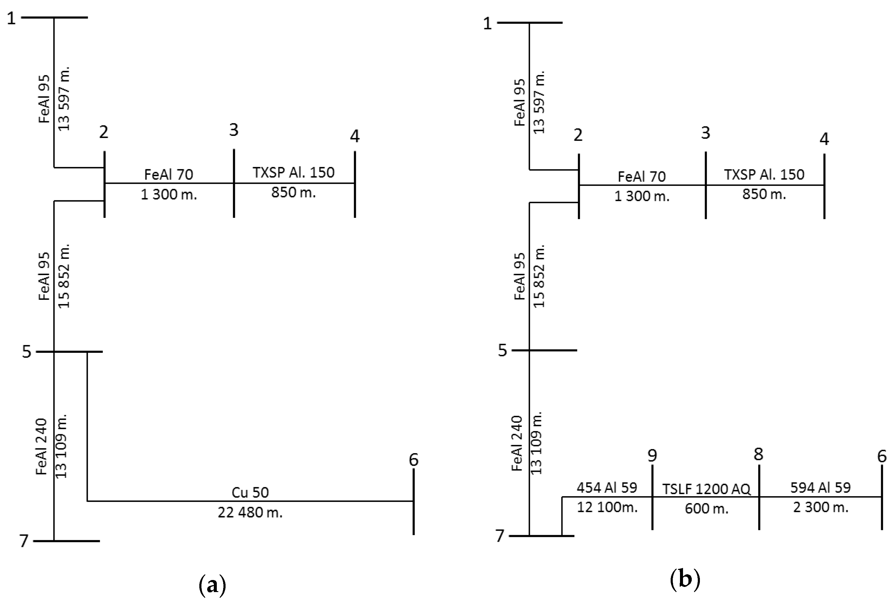
The run-on-river hydro power plant was connected to the existing grid in Node 4, cf. Figure 1a, and an agreement was put in place with a neighboring dam hydro power plant, connected to Node 1, to curtail the production at times when the thermal capacity of the grid was violated. This was seen as a temporary solution for the next 10 years because the existing connection line to the main grid (from Node 5 to Node 6) had to be replaced due to aging. Expensive investments could then be postponed through the use of active power curtailment. This was the chosen solution by the grid company in 2007, and the base case in our study. This strategy was possible in 2007 as the Norwegian regulation at that time was different from today.
2.2. Alternative 2: New Transmission Line
In this alternative, the transmission line between Nodes 5 and 6 in Figure 1a is replaced by a new transmission line between Nodes 6 and 7, whereas the old connection between Nodes 5 and 6 is torn down. The new grid configuration is illustrated in Figure 1b. The capacity in the grid is then sufficient for a worst-case scenario, so no active power curtailment is necessary. Other alternatives for grid upgrades were also considered, but this was the preferred solution by the DSO.
2.3. Overview of Loads and Production
The existing power plants are mainly located in node 1, the new run-on-river hydro power plant is connected to Node 4, and the load in the network is mainly located in Node 7. Node 6 represents the connection to the central transmission grid. The total amount of energy injected in to each node in 2013, i.e., the sum of the production and load under each node, is presented in Table 2. The grid is operated at 60 kV. More information on the loads and generation and time series measurements of the average power for each hour in each node can be found in Table S1 in Supplementary Materials.
3. Quantification of Costs for the Two Alternatives
3.1. Cost Components
The goal of this study is to analyze if there could be a socio-economic benefit of postponing the considered investment. The impacts for each different individual stakeholder are therefore not included, e.g., to which degree the DSO can compensate its investment costs by increasing the tariffs. The net present value, including all relevant socio-economic costs, was used to compare the two alternatives. The total cost for each alternative is shown in (1), where is the total cost for alternative j, is one cost component for alternative j, whereas I is the set of cost components.
Only cost types that were different in the two alternatives were included in the analysis, and all cost elements were determined in cooperation with the DSO responsible for the grid integration. The following cost components were included in the analysis:
- Investment cost for new line
- Tearing cost for old line
- Operations and maintenance cost
- Cost of transmission losses
- Cost of energy not supplied
In our case, there were no costs of lost energy from the developer’s perspective since it was the dam hydropower plant that curtailed production if needed. The corresponding compensation from the developer of the new run-on-river hydro power plant to the dam hydro power plant was regulated by an agreement between them. However, no such compensation was needed within the planning period. The cost of shifting some dam hydro power production away from the critical hours to other hours has therefore been set to zero in our study. This might be different in other cases, especially if no dam hydro power plants or, for example, flexible thermal power plants exist in the area. If there had been losses in production, it would be valuated at the producer price for electricity including any support for renewable generation.
Even if the considered area is well within one of the price zones in the Nordic system, the considered investment could in principle have some impact on the transmission capacity towards other price zones. However, it was taken as a premise that this impact and the corresponding costs would be minor in our case study.
3.2. Planning Period, Expectations, and Discounting
At the decision time in 2007, the expected remaining lifetime of the line between Nodes 5 and 6, cf. Figure 1a, was 10 years. The planning period when comparing the cost for the two alternatives was therefore set to 10 years, i.e., 2007–2016, after which the new line would be needed anyway. For several factors affecting costs (e.g., costs due to energy not supplied) observed values from the period 2007–2016 were applied rather than the corresponding expected values for each year in the next decade seen from 2007, since the expected values in many cases were hard to observe. The interest rate was set to 5% according to the interest rate at the decision time.
The present value of the yearly costs was calculated according to (2), where Ck is the yearly cost for each period, i is the interest rate, and n is the number of years.
In this case, the planning period was 10 years so k runs from 1 to 10 for annuity-immediate, i.e., the period when the cost occurred at the end of each period, while k runs from 0 to 9 for annuity-due, i.e., the cost occurs at the beginning of each period. If the cost occurred in the middle of the period, the average value of annuity-immediate and annuity-due was used.
3.3. Investment Cost
For the considered investment in a new line, the expected lifetime of the investment exceeded the planning period. The present value cost within the period of analysis was then calculated in two steps. Firstly, a yearly cost occurring in each year for the whole lifetime of the investment was calculated, with a present value equal to the overnight investment costs. The calculation of the yearly annuity was calculated according to (3), where C is the overnight investment cost, i is the interest rate, L is the lifetime, and A is the annual cost.
Secondly, the present value of the annual costs in the planning period was calculated according to (2), with constant yearly cost, i.e., . The estimated overnight investment cost in 2007 for the new line in Alternative 2 was 162 thousand € per km, and the length of the line was 15.5 km. The lifetime of the investment was set to 60 years. The corresponding present value of the annuity-immediate for the first 10 years was then 1030 thousand €.
3.4. Line Removal Cost
The estimated cost for removing the old line was 12.5 thousand € per km. It was assumed that the old line would be torn down as soon as the new line was ready for operation. Hence, for Alternative 1 the tearing cost was assumed to be due at the beginning of the planning period, and for Alternative 2 it is assumed to be due at the end of the planning period.
3.5. Operation and Maintenance Cost
The operation and maintenance cost for both the existing line between Nodes 5 and 6, and the proposed new line between Nodes 6 and 7 have been estimated. For the proposed new line between Nodes 5 and 6, the operation and maintenance cost was set to 1.5% of the investment cost per year over 40 years. This is a common practice for Norwegian grid companies. This gave a total present value of 663,230 €. It is assumed that the operation and maintenance cost would be equally distributed per year for the whole lifetime of the lines. As operation and maintenance costs typically occur at different times within a year, the costs were discounted as if they occurred in the middle of each year. This gave a present value in the first 10 years of 280 thousand €.
The yearly operation and maintenance cost for the existing line between Nodes 5 and 6 was calculated in two steps. Firstly, the annual costs were calculated with the methodology described for the new line, using an investment cost of 125 thousand € per km. Secondly, the level of maintenance performed on the line is expected to decrease towards the end of the lifetime on the basis that the line was to be torn down. A linear decrease from the level calculated in the first step down to zero in the final year was therefore estimated. This gave a present value of 170 thousand €.
3.6. Cost of Transmission Losses
To calculate the transmission losses, a model of the grid for the two alternatives was developed, and AC power flow simulations were performed for every hour between 2013 and 2015 based on measurements of injected power in the nodes provided by the DSO using the program package MATPOWER [26] in MATLAB®. Line data used in the model can be found in Appendix A. No major changes in production and consumption have occurred since 2007. By simulating three different years, we were to some extent able to take into account the impacts of climate variability, which is important in the hydropower-dominated Norwegian power system. The measurements of injected power can be found in Table S1 in Supplementary Materials. The total calculated transmission losses by the model during the three years was then used to calculate the average yearly energy losses. Measurements of reactive power were not available for the loads in Node 1 and part of the load in Node 7, so a power factor equal to 0.97 inductive was used for these loads.
Figure 2 compares the calculated losses per hour for Alternative 1 with the measured losses per hour (where the loss is the sum of the power injection in all nodes). The straight line indicates a perfect match between the calculated and measured losses. The figure shows that the difference between the calculated and the measured losses increased with the size of the losses. This deviation led to a slight underestimation of the yearly cost of transmission losses. The measured losses summed up to 47,371 MWh for the period 2013–2015 while the calculated losses were 43,955 MWh for the same period, i.e., calculated losses were 7.2% less than the measured losses. A similar comparison is not possible for Alternative 2 because this alternative is not yet realized. However, the underestimation would have existed for both alternatives and is therefore not expected to have a major influence on the difference in estimated losses between the two alternatives.
The calculated losses for each alternative and climate year is shown in Table 3. The monetary value of losses was calculated by the average day-ahead electricity price in the corresponding price zone on the Nordic power exchange Nord Pool in the period 2007–2015, i.e., 36 €/MWh [27]. This gave a present value for the cost of transmission losses of 4200 thousand € for Alternative 1, and 3620 thousand € for Alternative 2. The transmission loss is slightly underestimated in Alternative 2 relative to Alternative 1 for some hours since curtailment of generation would be avoided in this alternative, and thus the net injection would be higher in those hours. Needed curtailments were embedded in our measurement data for the net injection per node. Therefore, we could not know the number of curtailment instances.
3.7. Cost of Energy Not Supplied
The cost of energy not supplied (CENS) for Alternative 1 was set equal to the realized CENS due to faults on the line between Nodes 5 and 6 during the planning period (see Table S2 in Supplementary Materials). The calculation of CENS for Alternative 2 is shown in (4).
The symbols and represent the length of the overhead lines, as it is not expected any faults on the cable part of the new line due to aging or degradation during the planning period. The symbol i is an index for different CENS types, cf. Table 4. The symbol represents our assumptions for the expected CENS in Alternative 2 relative to Alternative 1, per km overhead line length:
- CENS due to lightning did not change due to the lines in the two alternatives having a similar construction regarding lightning protection, i.e.,
- CENS due to unexpected human activities did not change.
- CENS due to aging was reduced to zero in Alternative 2.
- CENS due to other technical failure was reduced by 50% in Alternative 2 because less faults are expected due to corrosion, rot, and wear with the new line.
- CENS due to wind and vegetation was reduced by 50% in Alternative 2, due to the new line being built with a larger phase distance and line height and in a more favorable area.
The CENS for the two alternatives are shown in Table 4. The present value of cost of energy not supplied was then calculated according to (2) for the two alternatives and it was assumed that the cost occurred in the middle of the periods.
3.8. Sensitivity Study
A sensitivity analysis was carried out to illustrate how different values for important input variables could affect results. The applied values are shown in Table 5. For electricity prices, the difference between the low and high value is roughly in accordance with the variation in annual average price in the considered 10-year period. For the transmission losses, the high and low values are set to represent the uncertainty in generation and load due to climate variability, and the uncertainties in the simulation model.
4. Results
Table 6 shows all included costs for the two alternatives. Notably, investment costs for the new line only occurred in Alternative 2. Transmission losses were higher in Alternative 1 because of a lower capacity in the grid. In total, building a new line was 330 thousand € more expensive. This amount was 13% of the overnight investment cost.
The impact of the sensitivities described in Table 5 on the extra cost of Alternative 2 compared to Alternative 1 is shown in Figure 3. From the figure, it can be seen that Alternative 1 is the most attractive solution for all sensitivities given in Table 5, except for low interest rate. Given the sensitivities in Table 5, it can also be seen that the investment cost, interest rate, and electricity price are the input parameters with the largest effect on the result of the case study.
5. Discussion
In this paper, a case study has been performed comparing two different alternatives to integrate a new run-on-river hydro power plant to the grid. A method for comparing different alternatives has been demonstrated and the important cost components have been quantified.
The investment cost for transmission lines is mainly determined by the terrain and availability of contractors. The investment cost for the new transmission line in Alternative 2 was estimated by the DSO based on their experience with building similar lines. The sensitivity study showed that the uncertainty in the investment cost could have a large effect on the results of the case study. However, in this case it is very unlikely that the investment cost would be so low that it would alter the conclusion of the case study.
The interest rate also had a major impact on results, as it shifted the relative importance of overnight investment costs vs. all other costs that were applied on a yearly basis. A low interest rate (from 3–5%, which is not very low in 2016) was the only sensitivity that gave lowest total cost for an investment in a new line.
From the results, it can be seen that transmission losses were the largest cost element for both alternatives, when all costs that were equal for both cases were left out. It can also be seen that a substantial reduction in cost due to transmission losses is achieved for the alternative with grid upgrade. In our case study, the replaced power line operated up to its thermal capacity only for a short period each year. In other cases where the grid is heavily loaded for larger periods of the year, grid upgrades might be a more attractive solution.
In this study, measurements of average energy injected into each node per hour were available. These measurements were used as an input in a power flow model to calculate the energy losses for the two alternatives. A comparison of the measured losses and the calculated losses for Alternative 1 showed that the simulations underestimated the losses by 7.2%. One possible explanation for this error was the simplifications made in the modelling of the reactive load, and inaccuracies in modelling of the electrical network i.e., accurate parameters for transmission lines, such as length. These inaccuracies were expected to be similar in both alternatives, so the margin of error was expected to be approximately the same for the calculation of the transmission losses in Alternative 2. From the sensitivity analyses, it can be seen that inaccuracies in the calculation of transmission losses in the considered range did not have a major impact on the final result compared to the uncertainties in other input parameters, such as investment costs.
Electricity prices affect the value of network losses, which was the largest cost factor in our study. Within the planning period, wholesale electricity prices have been falling in Europe due to several factors, including limited growth and increasing renewable power generation. It is possible that electricity prices will be considerably higher in the future, e.g., due to higher emission permit prices. A higher electricity price gives higher value of losses, and thus higher costs of postponing investments in the grid.
The reduction of cost of energy not supplied for the alternative with a new transmission line was difficult to estimate accurately, and estimates were based on guesses. One challenge is that an extraordinary event may lead to a large cost. In this study, a qualitative assessment has been done based on knowledge about the design of the new line in Alternative 2 and local weather conditions. The new line in Alternative 2 is expected to be less exposed to bad weather due to a more favorable location compared to the old line in Alternative 1. However, the sensitivity studies showed that the uncertainties considered in the cost elements for energy not supplied had relatively little effect compared to other cost factors.
The operation and maintenance cost was determined by the DSO based on their experience. There is great uncertainty associated with this cost. This cost type was however relatively small in both cases, and hence the sensitivity analysis showed that the uncertainty in the operation and maintenance cost only had a minor effect on the results.
In this case, the run-on-river hydro power plant made an agreement with a dam hydro power plant to curtail the production when the capacity of the grid was exceeded. As a part of this agreement the run-on-river hydro power plant should compensate the dam hydro power plant in cases were the active power curtailment lead to production loss or adverse production. In the period from 2007–2015 no compensation was necessary, i.e., the costs of production loss or adverse production were zero. In other cases, this might not be true. In cases were the active power production from renewable resources has to be curtailed, the cost of energy loss can be an important factor depending on the amount of time for which network congestion occurs.
6. Conclusions
The results show that, for this case, active power curtailment is socio-economically beneficial compared to grid upgrades. The alternative of applying active power curtailment had a socio-economic cost of 330 thousand € below the alternative involving grid upgrade in 2007. This equals 13% of the overnight investment cost. The main reason for the lower total costs of this alternative is cost savings due to postponed investment cost for grid upgrades, and no cost associated with production loss or adverse production due to the agreement with a dam hydro power plant to curtail the production.
Supplementary Materials
The following are available online at www.mdpi.com/1996-1073/10/5/632/s1, Table S1: Energy time series, Table S2: Cost of energy not supplied.
Acknowledgments
The work reported in this paper has been performed as part of the research project DGnett, founded by The Research Council of Norway, REN AS, and 13 Norwegian grid companies. The authors thank the partners in the project consortium for founding the project activities. The cost of publishing in open access has also been funded by the DGnett project. Finally, we thank Richard Hedger at Norwegian Institute for Nature Research for improving the English of the paper.
Author Contributions
Magne L. Kolstad and Ove Wolfgang conceived and designed the study, performed the calculations, analyzed the data, and wrote the paper; Rolf Håkan Josefsen jr. contributed with data material and analyzing the data.
Conflicts of Interest
The authors declare no conflict of interest. One of the authors represents one of the founding sponsors.
Appendix A

Table A1.
Line data including R and AC resistance referred to 20 °C and X: reactance in the positive and negative system.
Table A1.
Line data including R and AC resistance referred to 20 °C and X: reactance in the positive and negative system.
| Lines | R (Ω/km) | X (Ω/km) |
|---|---|---|
| FeAl 95 | 0.192 | 0.394 |
| FeAl 240 | 0.077 | 0.365 |
| FeAl 70 | 0.26 | 0.403 |
| TXSP Al 150 | 0.124 | 0.20 |
| Cu 50 | 0.357 | 0.43 |
| 454 Al 59 | 0.068 | 0.392 |
| TSLF 1200 AQ | 0.025 | 0.16 |
| 594 Al 59 | 0.53 | 0.384 |
References
- Interngovernmental Panel on Climate Change. Special Report on Renewable Energy Sources and Climate Change Mitigation; Cambridge University Press: New York, NY, USA, 2012. [Google Scholar]
- Driesen, J.; Belmans, R. Distributed generation: Challenges and possible solutions. In Proceedings of the 2006 IEEE Power Engineering Society General Meeting, Montreal, QC, Canada, 18–22 June 2006; p. 8. [Google Scholar]
- CIGRE Working Group C6.24. Capacity of Distribution Feeders for Hosting DER; CIGRE: Paris, France, 2014. [Google Scholar]
- Lopes, J.A.P.; Hatziargyriou, N.; Mutale, J.; Djapic, P.; Jenkins, N. Integrating distributed generation into electric power systems: A review of drivers, challenges and opportunities. Electr. Power Syst. Res. 2007, 77, 1189–1203. [Google Scholar] [CrossRef]
- Djapic, P.; Ramsay, C.; Pudjianto, D.; Strbac, G.; Mutale, J.; Jenkins, N.; Allan, R. Taking an active approach. IEEE Power Energy Mag. 2007, 5, 68–77. [Google Scholar] [CrossRef]
- Siano, P.; Chen, P.; Chen, Z.; Piccolo, A. Evaluating maximum wind energy exploitation in active distribution networks. IET Gener. Transm. Distrib. 2010, 4, 598–608. [Google Scholar] [CrossRef]
- CIGRE Working Group C6.19. Planning and Optimization Methods for Active Distribution Systems; CIGRE: Paris, France, 2014. [Google Scholar]
- Richardot, O.; Viciu, A.; Besanger, Y.; Hadjsaid, N.; Kieny, C. Coordinated Voltage Control in Distribution Networks Using Distributed Generation. In Proceedings of the 2005/2006 IEEE/PES Transmission and Distribution Conference and Exhibition, Dallas, TX, USA, 21–24 May 2006; pp. 1196–1201. [Google Scholar]
- Senjyu, T.; Miyazato, Y.; Yona, A.; Urasaki, N.; Funabashi, T. Optimal Distribution Voltage Control and Coordination with Distributed Generation. IEEE Trans. Power Deliv. 2008, 23, 1236–1242. [Google Scholar] [CrossRef]
- Elkhatib, M.E.; El-Shatshat, R.; Salama, M.M.A. Novel Coordinated Voltage Control for Smart Distribution Networks with DG. IEEE Trans. Smart Grid 2011, 2, 598–605. [Google Scholar] [CrossRef]
- Vovos, P.N.; Kiprakis, A.E.; Wallace, A.R.; Harrison, G.P. Centralized and Distributed Voltage Control: Impact on Distributed Generation Penetration. IEEE Trans. Power Syst. 2007, 22, 476–483. [Google Scholar] [CrossRef]
- Ault, G.W.; Currie, R. A.F.; McDonald, J.R. Active power flow management solutions for maximising DG connection capacity. In Proceedings of the 2006 IEEE Power Engineering Society General Meeting, Montreal, QC, Canada, 18–22 June 2006; p. 5. [Google Scholar]
- Currie, R.A.F.; Ault, G.W.; Fordyce, R.W.; MacLeman, D.F.; Smith, M.; McDonald, J.R. Actively Managing Wind Farm Power Output. IEEE Trans. Power Syst. 2008, 23, 1523–1524. [Google Scholar] [CrossRef]
- Tonkoski, R.; Lopes, L.A.C.; El-Fouly, T.H.M. Coordinated Active Power Curtailment of Grid Connected PV Inverters for Overvoltage Prevention. IEEE Trans. Sustain. Energy 2011, 2, 139–147. [Google Scholar] [CrossRef]
- Ochoa, L.F.; Dent, C.J.; Harrison, G.P. Distribution Network Capacity Assessment: Variable DG and Active Networks. IEEE Trans. Power Syst. 2010, 25, 87–95. [Google Scholar] [CrossRef]
- Liew, S.N.; Strbac, G. Maximising penetration of wind generation in existing distribution networks. IEE Proc.-Gener. Transm. Distrib. 2002, 149, 256–262. [Google Scholar] [CrossRef]
- Davidson, E.; Dolan, M.; Ault, G.; McArthur, S. AuRA-NMS: An autonomous regional active network management system for EDF energy and SP energy networks. In Proceedings of the 2010 IEEE Power and Energy Society General Meeting, Providence, RI, USA, 25–29 July 2010; pp. 1–6. [Google Scholar]
- Sansawatt, T.; Ochoa, L.F.; Harrison, G.P. Smart Decentralized Control of DG for Voltage and Thermal Constraint Management. IEEE Trans. Power Syst. 2012, 27, 1637–1645. [Google Scholar] [CrossRef]
- Gabash, A.; Li, P. Active-Reactive Optimal Power Flow in Distribution Networks with Embedded Generation and Battery Storage. IEEE Trans. Power Syst. 2012, 27, 2026–2035. [Google Scholar] [CrossRef]
- Ochoa, L.F.; Harrison, G.P. Minimizing Energy Losses: Optimal Accommodation and Smart Operation of Renewable Distributed Generation. IEEE Trans. Power Syst. 2011, 26, 198–205. [Google Scholar] [CrossRef]
- Gill, S.; Kockar, I.; Ault, G.W. Dynamic Optimal Power Flow for Active Distribution Networks. IEEE Trans. Power Syst. 2014, 29, 121–131. [Google Scholar] [CrossRef]
- Salih, S.N.; Chen, P.; Carlson, O.; Tjernberg, L.B. Optimizing Wind Power Hosting Capacity of Distribution Systems Using Cost Benefit Analysis. IEEE Trans. Power Deliv. 2014, 29, 1436–1445. [Google Scholar]
- Hu, Z.; Li, F. Cost-Benefit Analyses of Active Distribution Network Management, Part I: Annual Benefit Analysis. IEEE Trans. Smart Grid 2012, 3, 1067–1074. [Google Scholar] [CrossRef]
- Hu, Z.; Li, F. Cost-benefit analyses of active distribution network management, part II: Investment reduction analysis. IEEE Trans. Smart Grid 2012, 3, 1075–1081. [Google Scholar] [CrossRef]
- Gabash, A.; Xie, D.; Li, P. Analysis of influence factors on rejected active power from active distribution networks. In Proceedings of the IEEE Power and Energy Student Summit (PESS), Ilmenau, Germany, 19–20 January 2012; pp. 25–29. [Google Scholar]
- Zimmerman, R.D.; Murillo-Sanchez, C.E.; Thomas, R.J. MATPOWER: Steady-State Operations, Planning, and Analysis Tools for Power Systems Research and Education. IEEE Trans. Power Syst. 2011, 26, 12–19. [Google Scholar] [CrossRef]
- Nordpool. Available online: http://www.nordpoolspot.com/services/Power-Data-Services/Product-details/ (accessed on 18 April 2016).
Figure 1.
(a) One line diagram of the network as in alternative 1; (b) One line diagram of the network with the proposed new line as in alternative 2.
Figure 1.
(a) One line diagram of the network as in alternative 1; (b) One line diagram of the network with the proposed new line as in alternative 2.

Figure 2.
Calculated losses for Alternative 1 vs. actual losses (in MW) for all hours 2013–2015.
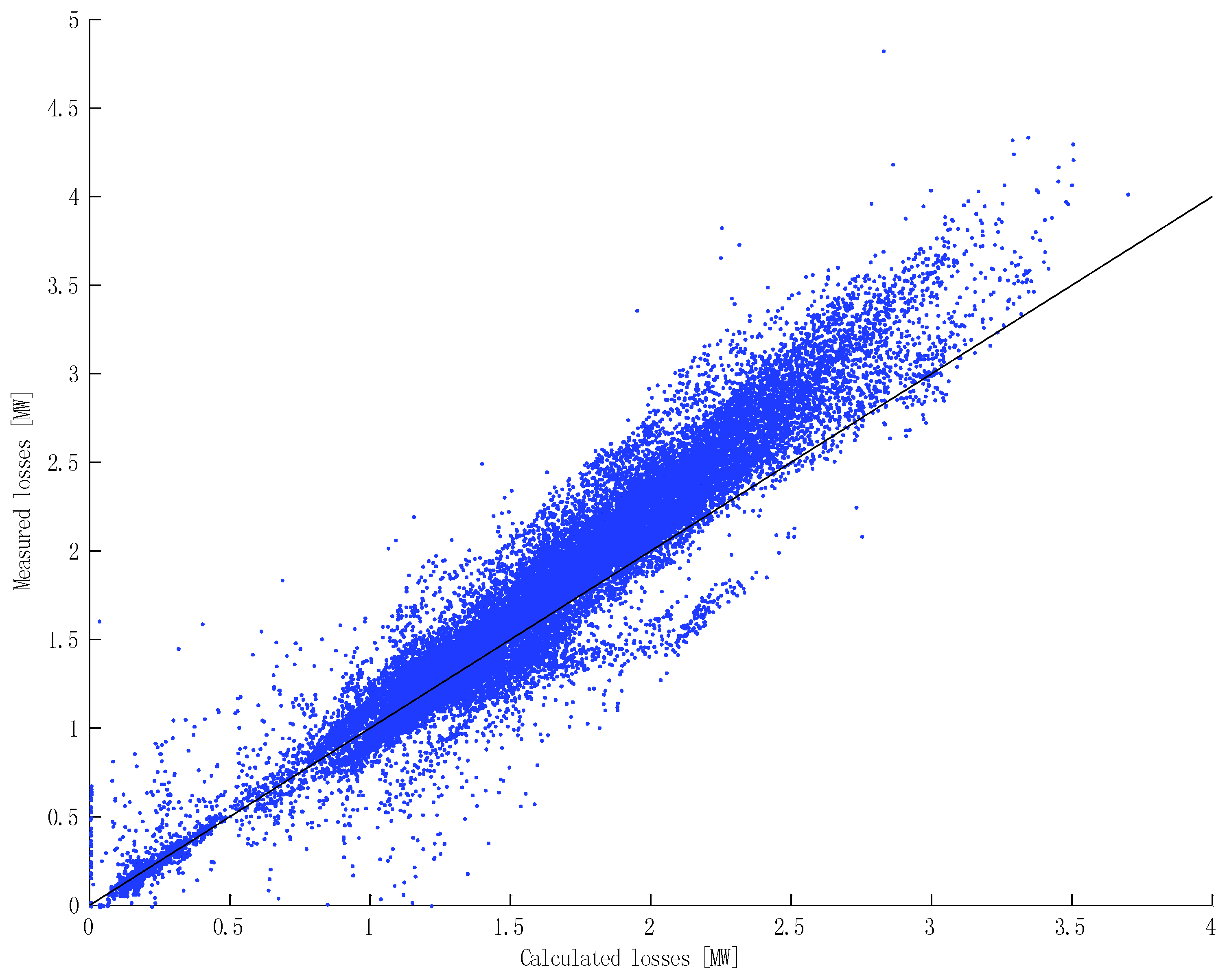
Figure 3.
Sensitivity analysis for single parameters (values in accordance with Table 5), and their impact on the extra cost of Alternative 2 (building a new line) compared to Alternative 1.
Figure 3.
Sensitivity analysis for single parameters (values in accordance with Table 5), and their impact on the extra cost of Alternative 2 (building a new line) compared to Alternative 1.
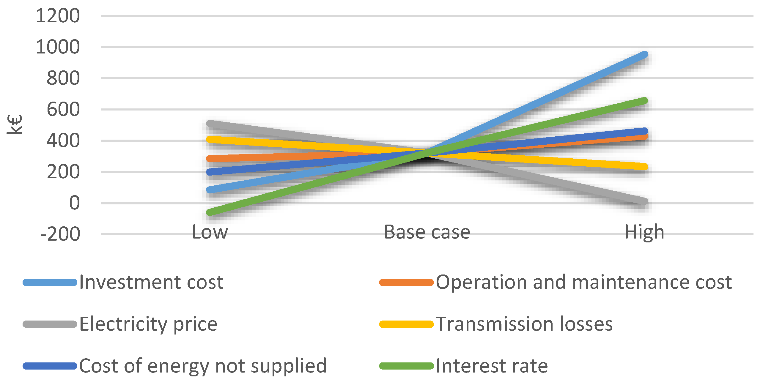
Table 1.
Capacity balance for the maximum generation-minimum load situation.
| Demand/Supply | Value (MW) |
|---|---|
| Existing generation | 32 |
| New generation | 8 |
| Light load | 6 |
| Losses | 2 |
| Required capacity out of area | 32 |
Table 2.
Total amount of energy injected in to each node in 2013, i.e., the sum of production and load under each node. Positive number indicates that the production exceeds the consumption. DSO: distribution system operator.
Table 2.
Total amount of energy injected in to each node in 2013, i.e., the sum of production and load under each node. Positive number indicates that the production exceeds the consumption. DSO: distribution system operator.
| Node | Balance (GWh) | Comment |
|---|---|---|
| Node 1 | 201.6 | Substation. A small village and several power plants |
| Node 2 | - | Joint |
| Node 3 | - | Joint |
| Node 4 | 30.9 | New run-on-river power plant |
| Node 5 | −6.8 | Reserve connection to neighboring DSO and a small load |
| Node 6 | −97.5 | Connection to the transmission grid |
| Node 7 | −114.9 | Substation. Small city. Reserve connection to neighboring DSO |
| Node 8 | - | Joint |
| Node 9 | - | Joint |
| Losses | 13.3 | - |
Table 3.
Calculated losses in MWh and cost of transmission losses for the two alternatives.
| Alternative | MWh | € | ||||
|---|---|---|---|---|---|---|
| Year | Average | Per Year | NPV 10 Years | |||
| 2013 | 2014 | 2015 | ||||
| Alternative 1 | 12,944 | 15,096 | 15,914 | 14,652 | 531,218 | 4,204,472 |
| Alternative 2 | 11,104 | 12,965 | 13,814 | 12,628 | 457,836 | 3,623,674 |
| Reduction | 1804 | 2131 | 2100 | 2027 | 73,382 | 580,798 |
Table 4.
Cost of energy not supplied for the two alternatives. CENS for Alternative 1 are based on realized values for the planning period, while the CENS for Alternative 2 are calculated based on the assumptions give above.
Table 4.
Cost of energy not supplied for the two alternatives. CENS for Alternative 1 are based on realized values for the planning period, while the CENS for Alternative 2 are calculated based on the assumptions give above.
| Cause | CENS Alternative 1 (€) | CENS Alternative 2 (€) |
|---|---|---|
| Lightning | 193,977 | 132,874 |
| Aging | 54,938 | 0 |
| Wind | 199,895 | 68,464 |
| Vegetation | 74,949 | 25,670 |
| Technical faults | 29,648 | 10,154 |
| Human activity | 61,006 | 41,789 |
| Total | 614,413 | 278,952 |
| Average yearly cost | 76,802 | 34,869 |
Table 5.
Applied parameter values in sensitivity analysis, compared to base case.
| Sensitivity Parameters | Low | Base Case | High |
|---|---|---|---|
| Investment cost | 112 k€/km | 162 k€/km | 250 k€/km |
| Operation and maintenance cost | 1% of investment cost over 40 years | 1.5% of investment cost in 40 years | 3% of investment cost in 40 years |
| Electricity price | 25 €/MWh | 36 €/MWh | 56 €/MWh |
| Transmission losses | Calculated losses reduced by 15% | See Table 3. | Calculated losses increased by 15% |
| Cost of energy not supplied | CENS due to technical errors or aging is zero | See Section 3.6. | CENS per km overhead line is the same as the old line. |
| CENS due to wind and vegetation is reduced by 90% | |||
| CENS due to lightning and unexpected human activity is reduced by 50% | |||
| Interest rate | 3% | 5% | 7% |
Table 6.
Present value costs for the two alternatives within the planning period (in thousand €).
| Cost | Alternative 1 | Alternative 2 |
|---|---|---|
| Investment cost | - | 1030 |
| Line removal cost | 170 | 280 |
| Operation and maintenance cost | 170 | 280 |
| Cost of transmission losses | 4200 | 3620 |
| Cost of energy not supplied | 610 | 270 |
| Total | 5150 | 5150 |
© 2017 by the authors. Licensee MDPI, Basel, Switzerland. This article is an open access article distributed under the terms and conditions of the Creative Commons Attribution (CC BY) license (http://creativecommons.org/licenses/by/4.0/).
Share and Cite
MDPI and ACS Style
Kolstad, M.L.; Wolfgang, O.; Josefsen, R.H. Case Study on the Socio-Economic Benefit of Allowing Active Power Curtailment to Postpone Grid Upgrades. Energies 2017, 10, 632. https://doi.org/10.3390/en10050632
AMA Style
Kolstad ML, Wolfgang O, Josefsen RH. Case Study on the Socio-Economic Benefit of Allowing Active Power Curtailment to Postpone Grid Upgrades. Energies. 2017; 10(5):632. https://doi.org/10.3390/en10050632
Chicago/Turabian StyleKolstad, Magne L., Ove Wolfgang, and Rolf Håkan Josefsen. 2017. "Case Study on the Socio-Economic Benefit of Allowing Active Power Curtailment to Postpone Grid Upgrades" Energies 10, no. 5: 632. https://doi.org/10.3390/en10050632
Note that from the first issue of 2016, this journal uses article numbers instead of page numbers. See further details here.