
Tidal Current Power Resources and Influence of Sea-Level Rise in the Coastal Waters of Kinmen Island, Taiwan


1
National Science and Technology Center for Disaster Reduction, New Taipei City 23143, Taiwan
2
Department of Geosciences, National Taiwan University, Taipei 10617, Taiwan
*
Author to whom correspondence should be addressed.
Energies 2017, 10(5), 652; https://doi.org/10.3390/en10050652
Submission received: 2 March 2017
/
Revised: 31 March 2017
/
Accepted: 4 May 2017
/
Published: 9 May 2017
(This article belongs to the Special Issue Marine Energy)
Abstract
:The tidal current power (TCP) resource, the impact of TCP extraction on hydrodynamics and the influence of sea-level rise (SLR) on TCP output in the coastal waters of Kinmen Island (Taiwan) are investigated using a state-of-the-art unstructured-grid depth-integrated numerical model. The model was driven by eight tidal constituents extracted from a global tidal prediction model and verified with time series of measured data for tide level and depth-averaged current. The simulations showed reasonable agreement with the observations; the skill index was in the excellent (0.71–0.93) range with regard to simulating tide level and currents. Model predictions indicated that the channel between Kinmen and Lieyu serves as an appropriate site for deploying the tidal turbines because of its higher tidal current and deeper water depth. The bottom friction approach was utilized to compute the average TCP over a spring-neap cycle (i.e., 15 days). Mean TCP reached its maximum to 45.51 kW for a coverage area of 0.036 km2 when an additional turbine friction coefficient (Ct) increased to 0.08, and a cut-in speed of 0.5 m/s was used. The annual TCP output was estimated to be 1.08 MW. The impact of TCP extraction on the change in current is significant, with a maximum reduction rate of instant current exceeding 60%, and the extent of influence for the average current is 1.26 km in length and 0.30 km in width for the −0.05 m/s contour line. However, the impact of TCP extraction on the change in tide level is insignificant; the maximum change in amplitude is only 0.73 cm for the K2 tide. The influence of SLR on the TCP output in Kinmen waters was also estimated. Modeling assessments showed that due to SLR produces faster tidal current, the annual TCP output increased to 1.52 MW, 2.01 MW, 2.48 MW and 2.97 MW under the same cut-in speed and coverage area conditions when SLR 0.25 m, SLR 0.5 m, SLR 0.75 m and SLR 1.0 m were imposed on the model.
1. Introduction
Global warming is expected to become more intense during this century due to the increasing emissions of greenhouse gases [1]. The relationship between the burning of fossil fuels and climate change is becoming more established. Therefore, renewable marine power resources, in the form of tides, waves, tidal currents and sea temperature (thermal energy), are potential candidates for possible energy sources [2,3]. The extraction of kinetic energy from tidal currents is a desirable form since it is predictable, regular, and has a high energy density with low greenhouse gas emissions [4].
Recently, many researchers have made great efforts to identify the most appropriate locations for the placement of tidal turbines and to assess how much tidal current power (TCP) can be extracted from a specific site [5,6,7]. Tidal currents are highly dependent on the geographic characteristics. For instance, a channel with varying cross-sections linking with two large water bodies is usually rich in TCP [5,6,7,8,9]. In addition, tidal currents can be accelerated in the area around a headland tip [10,11,12,13,14,15].
Although tidal turbine operation has less negative influences on the marine environment, the hydrodynamics of a tidal system, such as tide level and current speed, might change due to the extraction of TCP in a certain sea or estuarine area [2,16]. Thus, an assessment of the environmental impact should be conducted for a turbine farm before the deployment of tidal turbines. Although global warming may be far worse than thought and sea-level rise (SLR) is expected to accelerate over the next century [17,18], few studies have concentrated on estimating the effect of SLR on TCP output [19,20].
A numerical hydrodynamic model is a powerful tool to assess the distribution of TCP resources; a two-dimensional model (2D model) is required for shallow coastal waters [7,21,22], and a three-dimensional model (3D model) is required for the deep sea [2,23,24]. In addition, two approaches are commonly incorporated into numerical models to simulate the effect of TCP extraction on hydrodynamics. The first method is the bottom friction approach, and a 2D model is generally employed; the presence of tidal turbines in the water is represented by adding an additional bottom friction in the model [25,26]. The second method is the momentum-sink approach, which usually adopts a 3D model; in this model, the momentum is diminished by adding the TCP extraction effect terms in the momentum equations [2,23,24]. However, these two approaches produce similar results [24].
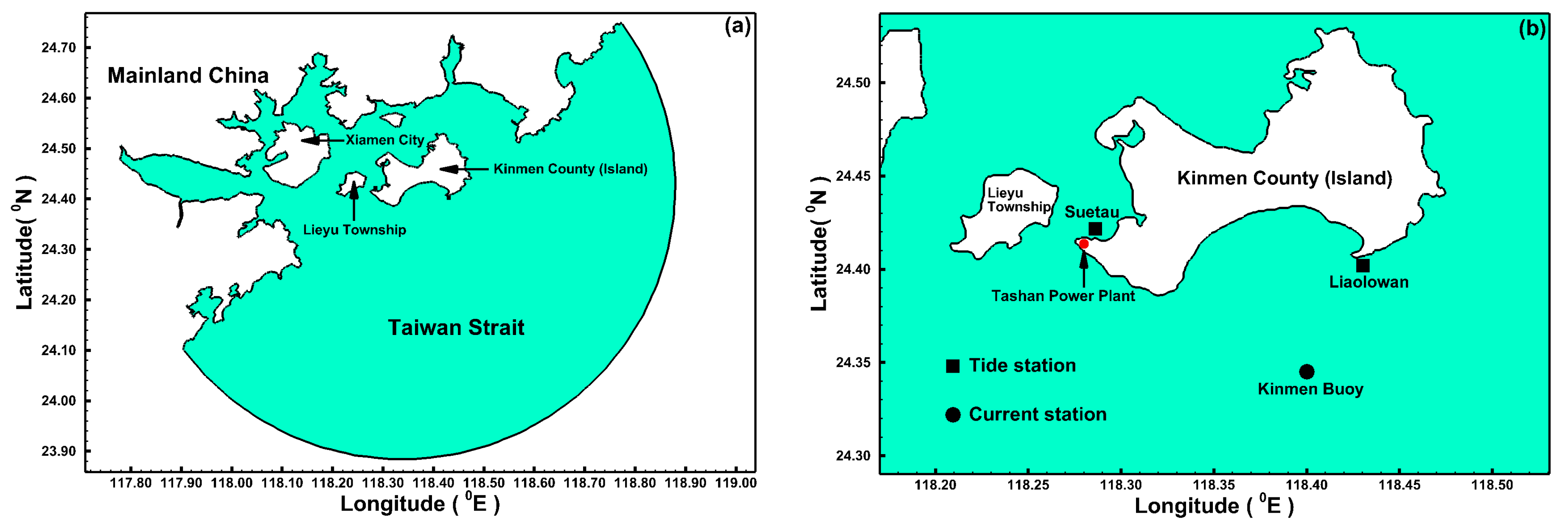
Kinmen Island (Kinmen Taiwan), located just off the southeastern coast of mainland China (Figure 1a), covers an area of 153 km2 and has a population of 135,223 (2017). The Tashan Power Plant (the red solid circle in Figure 1b) on Kinmen Island is a fuel-fired power plant built in 1967. The total power generation capacity of the Tashan Power Plant is approximately 34 MW. It is currently inadequate for meeting the power resource demand for the residents of Kinmen Island. Therefore, the TCP extracted from the coastal waters of Kinmen Island has been considered as an alternative power generation method because of its lower pollution.
The objectives of this study are as follows: (1) investigate the distribution of TCP resources and find an appropriate site for deploying the tidal turbines in the coastal waters of Kinmen Island; (2) calculate maximum mean TCP output over a spring-neap cycle using a high-resolution two-dimensional hydrodynamic model for the turbine site; (3) evaluate the impact of TCP extraction on the tide level and tidal current; and (4) assess the influence of SLR on TCP output.
2. Materials and Methods
2.1. Hydrodynamic Model
A state-of-the-art unstructured-grid hydrodynamic model called Semi-implicit Cross-scale Hydroscience Integrated System Model (SCHISM), has been used to simulate tide levels and tidal currents in the coastal waters of Kinmen Island. SCHISM is a modeling system that is a derivative product of the original SELFE model [27], with many enhancements and upgrades, including a new extension to the large-scale eddying regime and a seamless cross-scale capability from the creek to ocean scale [28].
Similar to the SELFE model, SCHISM is based on an unstructured grid and is designed for seamless simulation of three-dimensional baroclinic circulation across creek-lake-river-estuary-shelf-ocean scales. A highly efficient, parallel computing, robust and accurate semi-implicit finite-element/finite-volume method with an Eulerian-Lagrangian algorithm is implemented in the SCHISM model to solve Reynolds-averaged Navier-Stokes equations for transport of heat, salt and tracers. The wetting and drying scheme is naturally incorporated into the model for inundation studies. Due to their highly flexible frameworks, the SELFE and SCHISM models have been widely used to solve cross-scale problems: general circulation [29], storm surges [30], tsunami hazards [31], water quality [32], oil spills [33], sediment transport [34,35], biogeochemistry [36,37], and assessment of tidal stream energy resources [9,38]. A two-dimensional version of SCHISM, SCHISM-2D, is employed in this study since Kinmen Island is surrounded by shallow coastal waters (as shown in Figure 2a). The governing equations of the SCHISM-2D model with hydrostatic form and Boussinesq approximation in the Cartesian coordinate system are given as follows:
where is the free-surface elevation; and are the depth-averaged velocity in the direction, respectively; is the Coriolis factor; is the acceleration due to gravity; is the earth’s tidal potential; is the effective earth elasticity factor; is the density of water; is the atmospheric pressure at the free surface; and refer to the wind shear stress in the direction, respectively; and are the bottom shear stress in the direction, respectively; and , where is the bathymetric depth. The formulas of the bottom shear stress are as follows:
where is the bottom drag coefficient, which is determined through model validation. is an additional bottom friction coefficient introduced by tidal turbine. is equal to zero when turbine is absent; while is greater than zero when turbine is present.
2.2. Calculation of Tidal Current Power
The extractable TCP over a tidal cycle (spring-neap cycle) for a turbine can usually be estimated as follows:
where is the tidal power extraction rate in watts; is the number of turbines corresponding to the maximum average TCP output; is the turbine thrust coefficient; and is the swept area of the turbine. The over-bar above velocity term indicates the time average over a spring-neap cycle. Although Equation (5) has widely been used, the effects of additional bottom friction induced by turbine deployment on hydrodynamics cannot be appropriately represented. Garrett and Cummins [5] and Bryden and Couch [39] proposed that an additional drag term on the flow will arise from the deployment of turbines. The tidal current power output () can be evaluated considering the turbine-induced additional bottom friction coefficient () using the bottom friction approach [9,19,21,25,40]:
where is the area covered by the tidal turbine field; and are obtained from SCHISM-2D.
2.3. Model Configuration
The computational domain covers the entire Kinmen Islands group, including Kinmen and Lieyu, which are located just off the southeastern coast of mainland China and are surrounded by the Taiwan Strait (Figure 1a). A global gridded bathymetry dataset with a resolution of 30 arc-second obtained from the General Bathymetric Chart of the Oceans (GEBCO) was used in this study. It was generated by combining quality-controlled ship depth soundings with interpolation between sounding points guided by satellite-derived gravity data. The modeling domain is composed of 197,020 triangle mesh grid cells and 100,714 nodes. Coarse mesh with 1000 m resolution was arranged to open ocean boundaries in the Taiwan Strait, while fine mesh with 50 m resolution was used around Kinmen Island (Figure 2b). Once the unstructured grid was constructed, the gridded bathymetry data were interpolated to each node (Figure 2a). The SCHISM-2D model was driven by harmonic constants of eight major tidal constituents (M2, S2, N2, K2, K1, O1, P1, and Q1), which were extracted from the global inverse tidal model, TPXO [41,42]. A time step of 60 s was set to ensure the stability of the model. The initial conditions for the hydrodynamic model are the null free surface elevation and null velocity. Meteorological and hydrological conditions are not considered in the current study. The simulations were only run in barotropic mode, i.e., density gradients are excluded in the model.
2.4. Model Performance Indicators
Two criteria were used to evaluate the model performance for the simulation of tide level and the depth-averaged tidal current, which are the mean absolute percentage error (MAPE) and the skill [43]. It should be noted that the MAPE can only be used when there are no zero value among observations. The optimal value of the skill is 1, indicating perfect performance. A skill value ranging between 0.65 and 1.0 indicates excellent performance. Very good performance is in the range of 0.5–0.65; good performance is in the range of 0.2–0.5; and a skill value less than 0.2 expresses poor performance [44]:
where is the total number of data points; is the simulation value; is the measured data; and is the mean value of the measured data.
3. Results
3.1. Model Validation for Tide Level and Tidal Currents
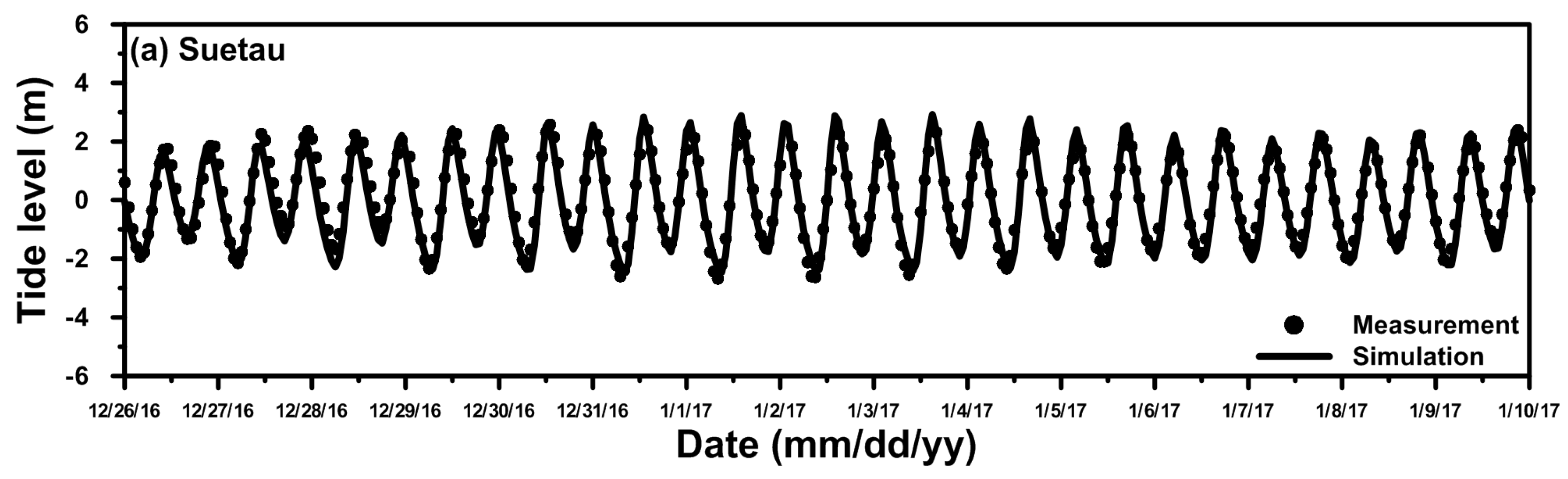
The observational data provided by the Taiwan Central Weather Bureau were used to validate the hydrodynamic model for predicting tide level and tidal currents (the gauging station locations are shown in Figure 1b). The date was measured during the winter (from December 2016 to January 2017); this means that the observations are not affected by severe weather conditions (e.g., typhoon). Although the northeast monsoon is sometimes stronger in this area in winter, the effects of winter monsoon winds on tide level and depth-averaged tidal current are not significant. Because the Kinmen buoy is placed at a location with the water depth of 20–25 m. In addition, the unusual values such as −9999.0 were also filtered. The simulation period, a total of 29 days, was from 12 December 2016 to 9 January 2017. The first 14 days are designed to confirm that the model results will not be affected by the initial conditions. Figure 3 shows the model-data comparison for tide level at Suetao (Figure 3a) and Liaolowan (Figure 3b). Excellent agreement between the simulated and measured time series of tide level is observed at these two tidal stations. The model performance in the tidal simulations is illustrated in Table 1. The MAPE and skill values are 17.68% and 0.93 for Suetao and 15.41% and 0.93 for Liaolowan, respectively.
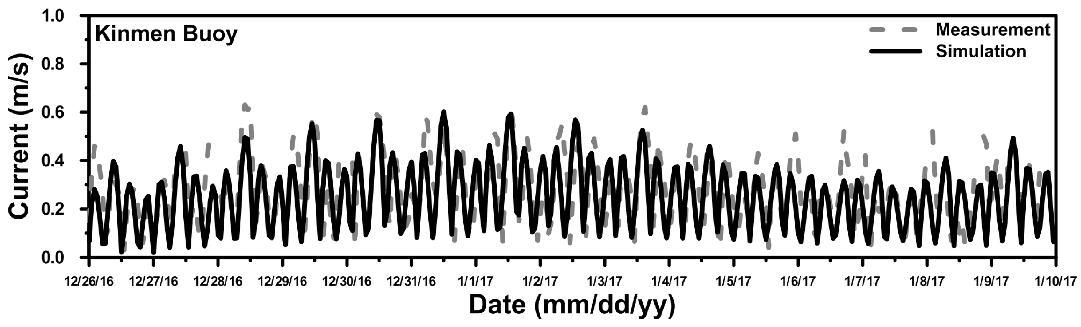
The predictions of the depth-averaged tidal currents for the Kinmen buoy were compared with the measurements; the comparison results are presented in Figure 4. The results reveal that the hydrodynamic model faithfully reproduces the peaks and phases of the tidal current. Table 1 indicates that the MAPE is 20.57%, and the skill score of 0.71 indicates an excellent performance of the tidal current simulations. The bottom drag coefficient () was determined as 0.002 through model validation. The SCHISM-2D model can therefore be practically applied to the TCP calculations.
The distribution of the average tidal current over a spring-neap cycle (i.e., 15 days) around Kinmen Island is shown in Figure 5a. A higher current is observed in a narrow channel between Kinmen and Lieyu, with a maximum current exceeding 2.0 m/s. This suggests that the area is appropriate for the deployment of tidal power turbines. Water depths in the range of 20–50 m are also a requirement, in addition to high tidal velocity [4]. Therefore, Figure 5b shows a desirable site (gray box), with an area of 35762.44 m2 (0.036 km2), depths greater than 20 m and average velocity of 0.43 m/s, for deploying the turbines.
3.2. Assessment of Maximum Tidal Current Power
According to a typical power curve, Robins et al. [45] assumed a cut-in velocity of 0.7 m/s and rated velocity of 2.7 m/s in the evaluation of tidal current power. However, this was an idealized representation of the potential performance of a turbine [46]. To assess the maximum potential TCP output in this study, the cut-in speed was therefore set to 0.5 m/s [47] and the rated velocity was not specified because the average tidal currents did not exceed 2.0 m/s at the turbine site.
The depth-averaged tidal currents were calculated by SCHISM-2D. TCP outputs were computed using Equations (6) and (7); the area covered by the tidal turbine field () was 35762.44 m2 (0.036 km2), and the turbine drag term () incrementally increased from 0.04 to 0.24. was added to in Equations (4a) and (4b), this means that the bottom shear stress would be increased with increasing , and consequently slow the horizontal velocity in the hydrodynamic model. Each simulation was carried out for each value of . In this way, the average TCP output over a spring-neap cycle increased with increasing , resulting in a reduction of the average velocity. There is a limit to the available TCP output as too many turbines not only create drag but also slow the current and therefore reduce the TCP output [4,17]. The maximum average TCP output is estimated to be 45.51 kW when , cut-in speed is 0.5 m/s, turbine coverage area is 35762.44 m2 and the average velocity is 0.33 m/s (as shown in Figure 6). This indicates that the annual TCP output was estimated to be 1.11 MW () at the turbine deployment site. The results shown in Figure 6 are similar to those of other studies for the calculations of TCP output using numerical models or theoretical methods [5,9,19,21].
3.3. Influence of Tidal Current Power Extraction on Hydrodynamics
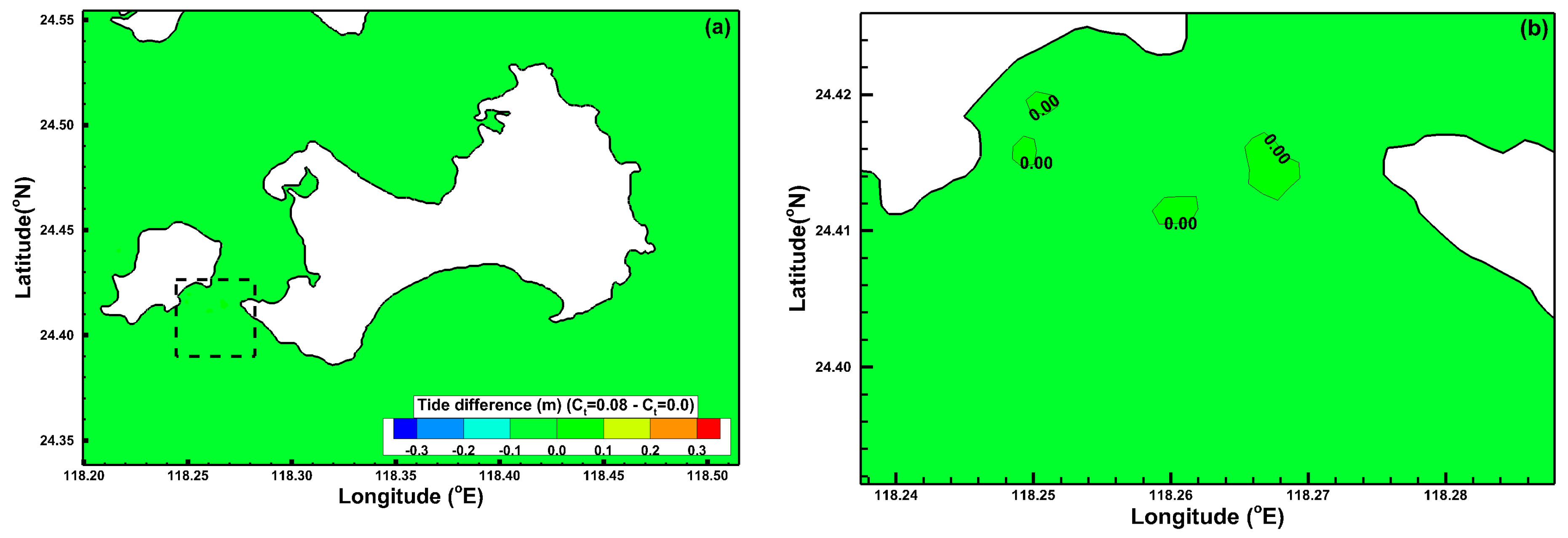
TCP extraction may alter the hydrodynamics (e.g., tide level and currents) over an area where the turbines are deployed. To understand the impacts of turbine operation on tidal dynamics, time series and spatial differences of tide level and currents were compared for an area with and without turbines. Due to produced the maximum mean TCP, Figure 7 depicts a tidal water level time series for and at the turbine site. The turbine-induced tide level change is minor; the difference is difficult to distinguish in Figure 7. The spatial distribution of tide level differences is shown in Figure 8a. The tide level difference at each node was obtained from the average tide level over a spring-neap cycle for minus that for . The differences in the average tide level between and in the spatial distribution are negligible, although an enlargement of the turbine site is shown in Figure 8b.
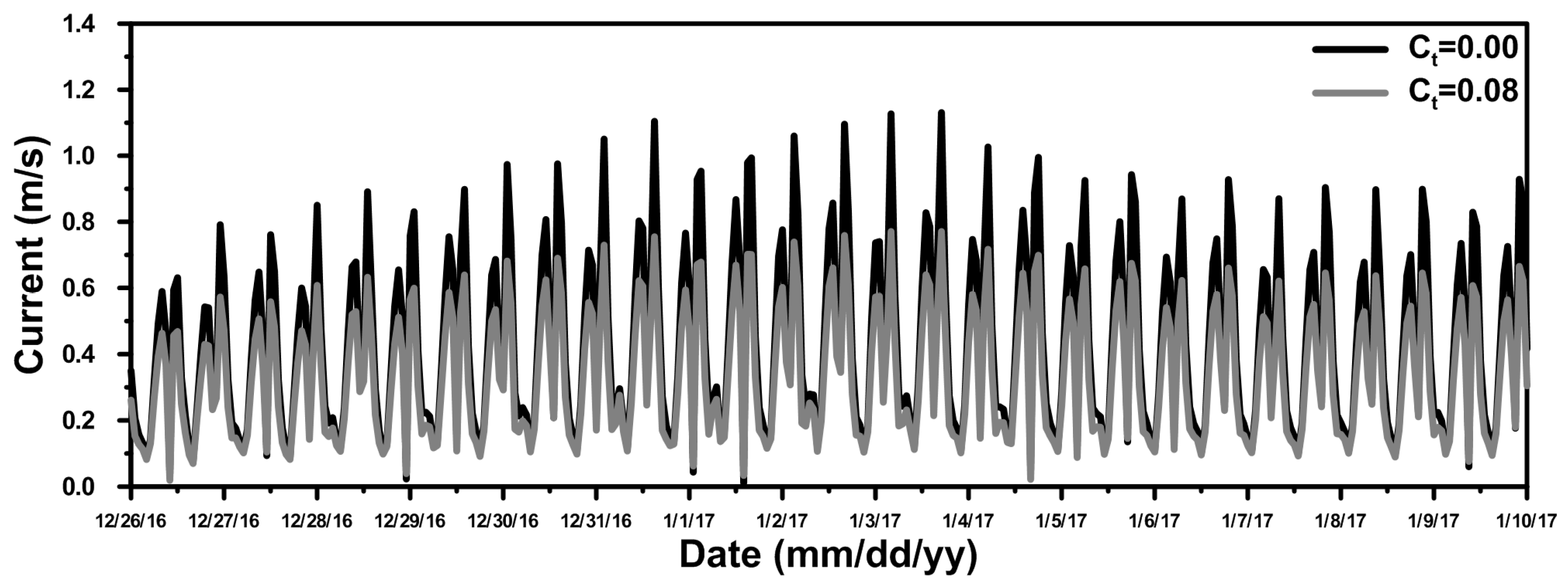
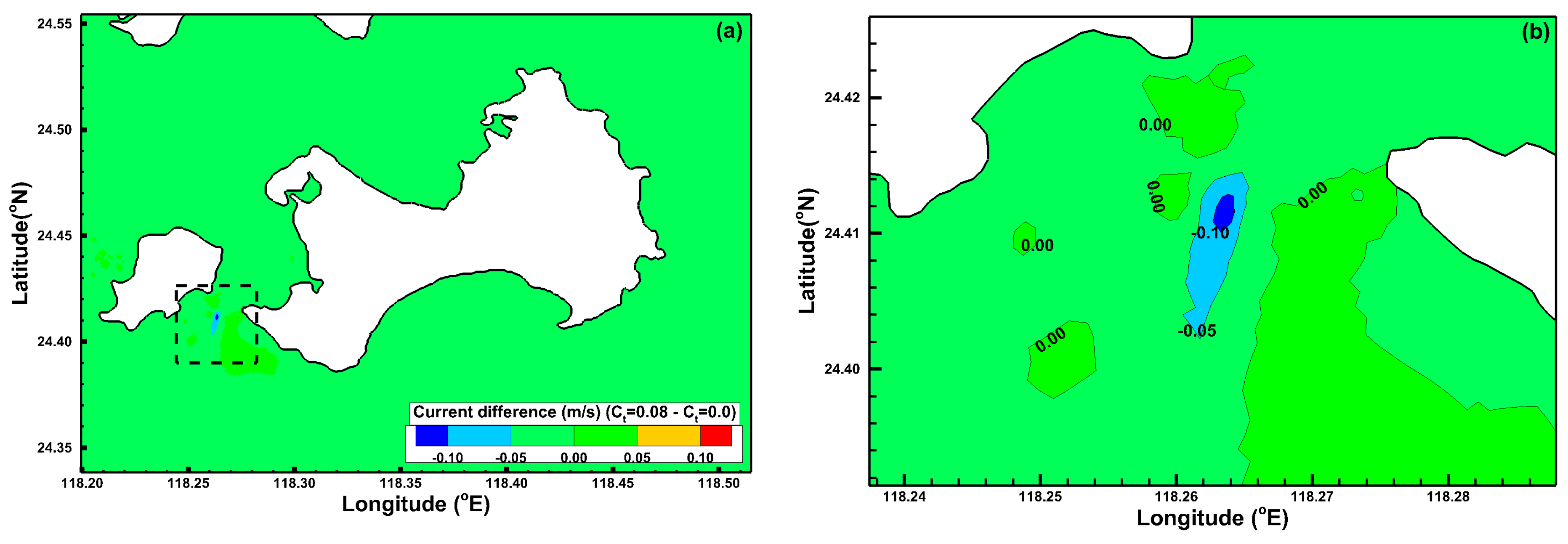
TCP extraction produced a very noticeable reduction in the tidal current. Figure 9 demonstrates a time series of the depth-averaged current for and at the turbine site. The maximum instant tidal current exceeded 1.1 m/s when the turbines are absent in the coastal waters; however, it was reduced to 68% due to the presence of tidal turbines (i.e., ). It is worth noting that the decrease in the time average tidal current was 77% for the comparison between and (as shown in Figure 6). Figure 10a exhibits the spatial distribution difference of the average tidal current over a spring-neap cycle for minus . The extent of the influence is 0.30 km in length and 0.13 km in width for the −0.10 m/s contour line, and 1.26 km in length and 0.30 km in width for the −0.05 m/s contour line (as shown in Figure 10b). The installment of turbines not only significantly retards the tidal current but also affects a certain area adjacent to the TCP extraction site.
3.4. Influence of Sea-Level Rise on Tidal Current Power Output
According to the Intergovernmental Panel on Climate Change (IPCC) AR5 report, the sea levels could rise 0.26 m to 0.54 m for RCP 2.6; 0.32 m to 0.62 m for RCP 4.5; 0.33 m to 0.62 m for RCP6.0; and 0.45 m to 0.81 m for RCP8.5 by 2100 [48]. Therefore the effects of SLR on TCP output were assessed by conducting the scenario simulations for SLR 0.25 m, SLR 0.5 m, SLR 0.75 m and SLR 1.0 m. We assumed that the tidal dynamics outside of the study region do not change. All boundary and bathymetry conditions are kept constant except for increasing the water depth by 0.25 m, 0.5 m, 0.75 m and 1.0 m over the entire computational domain and open boundaries. This straightforward approach has been widely adopted to investigate the effects of SLR on coastal hydrodynamics and tidal energy resources [19,44,49,50]. TCP outputs were also calculated by Equations (6) and (7) with an incremental , a cut-in speed of 0.5 m/s and of 35762.44 m2; the depth-averaged tidal currents were obtained from the outputs of SCHISM-2D.
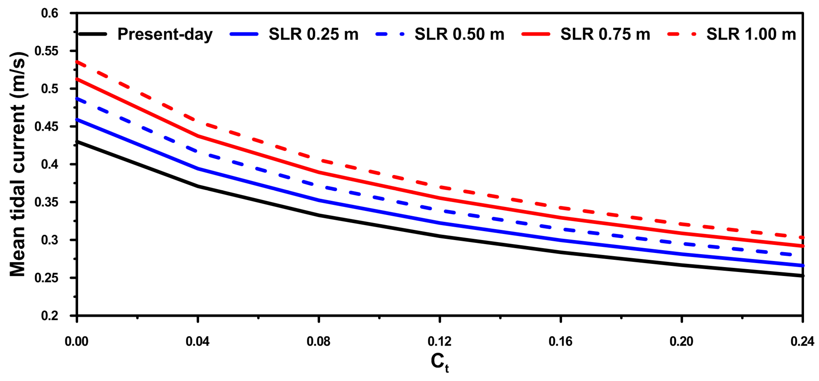
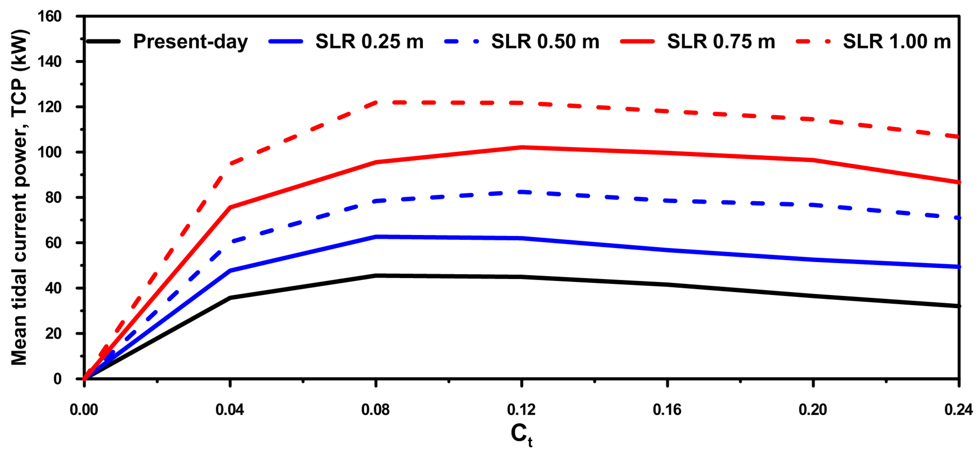
Figure 11 illustrates the average TCP outputs corresponding to different values. The maximum average TCP output is evaluated to be 62.64 kW, 82.43 kW, 102.12 kW and 121.94 kW for SLR 0.25 m, SLR 0.5 m, 0.75 m and SLR 1.0 m. Compared to present-day sea level, the annual TCP output increased to 1.52 MW, 2.01 MW, 2.48 MW and 2.97 MW under the SLR 0.25 m, SLR 0.5 m, SLR 0.75 m and SLR 1.0 m scenarios, respectively. This means that SLR produces higher TCP due to the faster tidal current at the turbine site in the coastal waters of Kinmen Island (Figure 12).
4. Discussion and Future Work
The effect of TCP extraction on the change in tide level is difficult to determine in the time series and spatial difference figures (Figure 7 and Figure 8). To quantify TCP extraction impact on tide level change, harmonic analysis was conducted to extract the main eight tidal components for (without TCP output) and (with maximum mean TCP output) at the turbine site. Table 2 lists the amplitudes and phases of eight tidal constituents for and . The maximum changes in amplitude and phase caused by turbines are only 0.73 cm and 0.77° for the K2 tide, respectively. The change of tide level for TCP extraction is ignored in both qualitative and quantitative analyses. Yang and Wang [51] compared the tide level changes of a tidal channel with and without turbines. They found that TCP extraction had a minor influence on the tidal elevations. Defne et al. [2] assessed the effects of TCP extraction on water level for an estuarine area, they concluded that both the decrease in the maximum water level and the increase in the minimum are kept below 0.05 m. Chen et al. [38] estimated the influences of TCP extraction on water level for the Taiwan Strait using the momentum sink approach. Their study results found that TCP extraction at a specific farm could significantly affect the tidal current, but the change in tidal amplitude and tidal phase could be neglected. Plew and Stevens [52] also suggested that introducing turbines in the numerical model has only a minor influence on the difference in water level through the Tory Channel. This phenomenon might be due to the water level simulations are mainly determined by the tide elevations specified at open boundaries.
According to the numerical experiments conducted in Section 3.4, the maximum average TCP was increased with SLR because a higher sea level produces faster tidal currents (as shown in Figure 12). The momentum equations in Equations (2) and (3) can be used to explain this phenomenon. The last term on the right-hand side of Equations (2) and (3) shows that the horizontal velocities, and , are proportional to the total water depth () when the wind shear stresses ( and ) are excluded in the model. In other words, deeper water depth (i.e., SLR) leads to faster tidal currents if the bottom drag coefficient remains constant. Lopes and Dias [53] estimated the impacts of SLR on tidal dynamics for the Ria de Aveiro lagoon in Portugal, using the ELCIRC 2D model. Chen and Liu [9] assessed the influences of SLR on tidal energy output for the Taiwan Strait. The same findings were also found in their studies, suggesting that SLR produces faster tidal currents and consequently increases TCP output.
Uehara et al. [54] used a two-dimensional model to investigate tidal and tide-dependent changes in the northwest European shelf seas over the last twenty thousand years. They adopted two approaches to consider the effect of future ocean-tide variability on the open boundary of the numerical model. One is fixed to the present state; the other is variable according to a global paleotidal model. They found that the M2 amplitude only increases by 1.0 m (0.9–1.9 m) in the west of the Celtic Sea through twenty thousand years. Although more realistic changes in shelf tides during ten thousand years can be obtained in this way, the variation of tidal amplitude might be small 100 years from now. It would be sensible to assume that the change of tidal amplitudes from 2017 to 2100 is ignorable. Therefore, we compared the TCP output between present-day sea level and future SLR using the same boundary conditions in the model. However, modeling assessment of future hydrodynamics might be more faithful if accurate projections of future tide variations for model boundary conditions are available.
Pelling and Green [19] conducted a series of numerical experiments to assess the SLR influence on TCP output for the Gulf of Maine. In their study, SLR was implemented according to two approaches. The first approach was to increase the water depth over the entire model domain and allow low-lying elements on the land to be flooded (referred to as the ‘flood run’). The second method was the same as the first except that no area was allowed to be flooded (referred to as the ‘no-flood run’). They found that the no-flood run produced higher maximum power output than the flood run for the Minas Passage. This is because TCP became dissipated when new shallow-water areas were created in the flood run. The difference in maximum TCP output is only 8.7% between these two approaches for the Minas Passage. Ward et al. [49] used the flood run method to investigate the impact of SLR on tidal dynamics for the European shelf; they also suggested that different way to implement SLR in the model shown a significant effect on response of tide. Although the flood run approach is much more realistic than the no-flood run approach, we can only adopt the latter due to the scarcity of accurate topography data and land-use data for Kinmen Island and Lieyu Island. In other words, we can suppose that an actual average maximum TCP might be 41.55 kW ( kW) in the Kinmen coastal waters if the flood run were used.
Due to the amount of TCP output is small and semi-diurnal intermittency of tidal current at the turbine deployment site in the Kinmen coastal waters; it might be possible to conduct storage into the supergrid [15,55]. Besides, Neill et al. [56] proposed that optimization of the TCP and finding the optimal site for parallel development for relative low number of arrays are import for large scale exploitation of TCP and should be conducted in the future work. In addition, Lewis et al. [57] found that the wave-current interaction could potentially alter tidal currents and should be included in hydrodynamic models in future studies.
Using a combination of Equations (5) and (7) to obtain the number of turbines is too simple when maximum mean TCP output was given. Myers and Bahaj [58] and Mestres et al. [59] suggested that the separation between both rows is taken as 10 times the dimeter of the tidal turbine rotor and the inter-lateral turbine separation 2.5 times the diameter. The configuration of tidal turbine array should be carefully considered before the construction of tidal turbine farm; however this requires further examination, which is beyond the scope of this paper.
5. Conclusions
The hydrodynamics in the coastal waters of Kinmen Island have been simulated using a state-of-the-art unstructured-grid depth-integrated numerical model, SCHISM-2D. The simulations were verified with tide level and depth-averaged tidal current measurements, showing a reasonable agreement with the observations. The validated model was then applied to evaluate TCP resources and appropriate sites for deploying tidal turbines around the coastal waters of Kinmen Island. A narrow channel between Kinmen and Lieyu was found to be a suitable area for turbine deployment because of its higher mean tidal current. The site has an area of 0.036 km2, depth greater than 20 m and average velocity of 0.43 m/s, making it suitable as a tidal current turbine farm. The bottom friction approach was employed to calculate the mean TCP over a spring-neap cycle. The maximum average TCP output is estimated as 45.51 kW when the additional turbine friction coefficient , cut-in speed is 0.5 m/s and average velocity is 0.33 m/s. The impacts of TCP extraction on hydrodynamics were also estimated. The TCP extraction effect can be ignored for tide level but shows a significant reduction in tidal currents. We found that the installation of turbines not only retarded tidal currents but also affected a certain area near the TCP extraction site. Four SLR scenarios, SLR 0.25 m, SLR 0.5 m, SLR 0.75 m and SLR 1.0 m, were conducted to investigate the influence of SLR on TCP output. Compared to the present-day sea-level condition, the annual TCP output increased to 1.52 MW, 2.01 MW, 2.48 MW and 2.97 MW for SLR 0.25 m, SLR 0.5 m, SLR 0.75 m and SLR 1.0 m, respectively, due to the faster tidal current. Acceptable simulations of tidal dynamics for the coastal waters of Kinmen Island were accomplished in this study, however, there are still many uncertainties associated with tidal current simulations, and TCP calculation should be further considered in the future.
Acknowledgments
This research was funded by the Ministry of Science and Technology (MOST), Taiwan, grant No. MOST 105-2625-M-865-002. The authors would like to thank the Central Weather Bureau, Taiwan, for providing the measurements, and Joseph Zhang of the Virginia Institute of Marine Science, College of William & Mary, for kindly sharing his experiences of using the numerical model.
Author Contributions
Hongey Chen, Lee-Yaw Lin, Yi-Chiang Yu and Wei-Bo Chen conceived the study, and Wei-Bo Chen performed the model simulations. The final manuscript has been read and approved by all authors.
Conflicts of Interest
The authors declare no conflict of interest.
References
- Solomon, S.; Qin, D.; Manning, M.; Chen, Z.; Marquis, M.; Averyt, K.B.; Tignor, M.; Miller, H.L. Climate Change 2007: The Physical Science Basis. Contribution of Working Group I to the Fourth Assessment Report of the Intergovernmental Panel on Climate Change; Cambridge University Press: Cambridge, UK, 2007. [Google Scholar]
- Defne, Z.; Hass, K.A.; Fritz, H.M. Numerical modeling of tidal currents and the effects of power extraction on estuarine hydrodynamics along the Georgia coast, USA. Renew. Energy 2011, 36, 3461–3471. [Google Scholar] [CrossRef]
- Lewis, M.J.; Angeloudis, A.; Robins, P.E.; Evans, P.S.; Neill, S.P. Influence of storm surge on tidal range energy. Energy 2017, 122, 25–36. [Google Scholar] [CrossRef]
- Lewis, M.; Neill, S.P.; Robins, P.E.; Hasheme, M.R. Resource assessment for future generations of tidal-stream energy arrays. Energy 2015, 83, 403–415. [Google Scholar] [CrossRef]
- Garrett, C.; Cummins, P. The power potential of tidal currents in channels. Proc. R. Soc. A 2005, 461, 2563–2572. [Google Scholar] [CrossRef]
- Polagye, B.; Kawase, M.; Malte, P. In-stream tidal energy potential of Puget Sound, Washington. Proc. Inst. Mech. Eng. Part A 2009, 223, 571–587. [Google Scholar] [CrossRef]
- Walkington, I.; Burrows, R. Modelling tidal stream power potential. Appl. Ocean Res. 2009, 31, 239–245. [Google Scholar] [CrossRef]
- Chen, W.-B.; Liu, W.-C.; Hsu, M.-H. Modeling assessment of tidal current energy at Kinmen Island, Taiwan. Renew. Energy 2013, 50, 1073–1082. [Google Scholar] [CrossRef]
- Chen, W.-B.; Liu, W.-C. 2017 Assessing the influence of sea level rise on tidal power output and tidal energy dissipation near a channel. Renew. Energy 2017, 101, 603–616. [Google Scholar] [CrossRef]
- Carballo, R.; Iglesias, G.; Castro, A. Numerical model evaluation of tidal stream energy resources in the Ria de Muros (NW Spain). Renew. Energy 2009, 34, 1517–1524. [Google Scholar] [CrossRef]
- Xia, J.; Falconer, R.A.; Lin, B. Numerical model assessment of tidal stream energy resources in the Severn Estuary, UK. Proc. Inst. Mech. Eng. Part A 2010, 224, 969–983. [Google Scholar] [CrossRef]
- Blunden, L.S.; Bahaj, A.S.; Aziz, N.S. Tidal current power for Indonesia? An initial resource estimation for the Alas Strait. Renew. Energy 2013, 49, 137–142. [Google Scholar] [CrossRef]
- Chen, Y.; Lin, B.; Lin, J.; Wang, S. Effect of stream turbine array configuration on tidal current energy extraction near an island. Comput. Geosci. 2015, 77, 20–28. [Google Scholar] [CrossRef]
- Robins, P.E.; Neill, S.P.; Lewis, M.J.; Ward, S.L. Characterising the spatial and temporal variability of the tidal-stream energy resources over the northwest European shelf seas. Appl. Energy 2015, 147, 510–522. [Google Scholar] [CrossRef]
- Easton, M.C.; Woolf, D.K.; Bowyer, P. The dynamics of an energetic tidal channel, the Pentland Firth, Scotland. Cont. Shelf Res. 2012, 48, 50–60. [Google Scholar] [CrossRef]
- Neill, S.P.; Jordan, J.R.; Couch, S.J. Impact of tidal energy converter (TEC) arrays on the dynamics of headland sand. Renew. Energy 2012, 37, 387–397. [Google Scholar] [CrossRef]
- Church, J.A.; White, N.J. A 20th century acceleration in global sea-level rise. Geophys. Res. Lett. 2006, 33, L01602. [Google Scholar] [CrossRef]
- Woodworth, P.; Gehrels, W.; Nerem, R. Nineteenth and twentieth century changes in sea level. Oceanography 2011, 24, 80–93. [Google Scholar] [CrossRef]
- Pelling, H.E.; Green, A.M. Sea level rise and tidal power plants in the Gulf of Maine. J. Geophys. Res. Ocean. 2013, 118, 2863–2873. [Google Scholar] [CrossRef]
- Tang, H.S.; Kraatz, S.; Qu, K.; Chen, G.Q.; Aboobaker, N.; Jiang, C.B. High-resolution survey of tidal energy towards power generation grid and influence of sea-level-rise: A case study at coast of New Jersey, USA. Renew. Sustain. Energy Rev. 2014, 32, 960–982. [Google Scholar] [CrossRef]
- Karsten, R.; McMillan, J.; Lickley, M.; Haynes, R. Assessment of tidal current energy in the Minas Passage, Bay of Fundy. Proc. Inst. Mech. Eng. Part A 2008, 222, 493–507. [Google Scholar] [CrossRef]
- Draper, S.; Houlsby, G.; Oldfield, M.; Borthwick, A. Modeling tidal energy extraction in a depth-averaged coastal plain. In Proceedings of the 8th European Wave and Tidal Energy Conference, Uppsala, Sweden, 7–10 September 2009. [Google Scholar]
- Hasegawa, D.; Sheng, J.; Greenburg, D.A.; Thompson, K.R. Far-field effects of tidal energy extraction in the Minas Passage on tidal circulation in the Bay of Fundy and Gulf of Maine using a nested-grid coastal circulation model. Ocean Dyn. 2011, 61, 1845–1868. [Google Scholar] [CrossRef]
- Yang, Z.; Wang, T.; Copping, A.E. Modeling tidal stream energy extraction and its effect on transport processes in a tidal channel and bay system using a three-dimensional coastal ocean model. Renew. Energy 2013, 50, 605–613. [Google Scholar] [CrossRef]
- Sutherland, G.; Foreman, M.; Garrett, C. Tidal current energy assessment for Johnstone Strait, Vancouver Island. Proc. Inst. Mech. Eng. Part A 2007, 221, 147–157. [Google Scholar] [CrossRef]
- Atwater, J.; Lawrence, G. Power potential of a split channel. Renew. Energy 2010, 35, 329–332. [Google Scholar] [CrossRef]
- Zhang, Y.; Baptista, A.M. SELFE: A semi-implicit Eulerian-Lagrangian finite-element mode for cross-scale ocean circulation. Ocean Model. 2008, 21, 71–96. [Google Scholar] [CrossRef]
- Zhang, Y.; Ye, F.; Stanev, E.V.; Grashorn, S. Seamless cross-scale modelling with SCHISM. Ocean Model. 2016, 102, 64–81. [Google Scholar] [CrossRef]
- Zhang, Y.; Ateljevich, E.; Yu, H.S.; Wu, C.H.; Yu, J.C.S. A new vertical coordinate system for a 3D unstructured-grid model. Ocean Model. 2015, 85, 16–31. [Google Scholar] [CrossRef]
- Bertin, X.; Li, K.; Roldan, A.; Zhang, Y.J.; Breilh, J.F.; Chaumillion, E. A modeling-based analysis of the flooding associated with Xynthia, central Bay of Biscay. Coast. Eng. 2014, 94, 80–89. [Google Scholar] [CrossRef]
- Zhang, Y.; Witter, R.; Priest, G.R. Tsunami-tide interaction in 1964 Prince William Sound tsunami. Ocean Model. 2011, 40, 246–259. [Google Scholar] [CrossRef]
- Chen, W.; Liu, W. Investigating the fate and transport of fecal coliform contamination in a tidal estuarine system using a three-dimensional model. Mar. Pollut. Bull. 2017, 116, 365–384. [Google Scholar] [CrossRef] [PubMed]
- Azevedo, A.; Oliverira, A.; Fortunato, A.B.; Zhang, Y.; Baptista, A.M. A cross-scale numerical modeling system for management support of oil accidents. Mar. Pollut. Bull. 2014, 80, 132–147. [Google Scholar] [CrossRef] [PubMed]
- Pinto, L.; Fortunato, A.B.; Zhang, Y.; Oliverira, A.; Sancho, F.E.P. Development and validation of a three-dimensional morphodynamic modelling system. Ocean Model. 2012, 57–58, 1–14. [Google Scholar]
- Chen, W.-B.; Liu, W.-C.; Hsu, M.-H.; Hwang, C.-C. Modelling investigation of suspended sediment transport in a tidal estuary using a three-dimensional model. Appl. Math. Model. 2015, 39, 2570–2586. [Google Scholar] [CrossRef]
- Rodrigues, M.; Oliveira, A.; Queiroga, H.; Fortunato, A.B.; Zhang, Y.J. Three-dimensional modeling of the lower trophic levels in the Ria de Aveiro (Portugal). Ecol. Model. 2009, 220, 1274–1290. [Google Scholar] [CrossRef]
- Rodrigues, M.; Oliveira, A.; Guerreior, M.; Fortunato, A.B.; Menaia, J.; David, L.M.; Cravo, A. Modeling fecal contamination in the Aljezur coastal stream (Portugal). Ocean Dyn. 2011, 61, 841–856. [Google Scholar] [CrossRef]
- Chen, W.B.; Liu, W.C.; Hsu, M.H. Modeling evaluation of tidal stream energy and the impacts of energy extraction on hydrodynamics in the Taiwan Strait. Energies 2013, 6, 2191–2203. [Google Scholar] [CrossRef]
- Bryden, I.G.; Couch, S. ME1-marine energy extraction: Tidal resource analysis. Renew. Energy 2006, 31, 133–139. [Google Scholar] [CrossRef]
- Blanchfield, J.; Garrett, C.; Wild, P.; Rowe, A. The extractable power from a channel linking a bay to the open ocean. Proc. Inst. Mech. Eng. Part A 2008, 222, 289–297. [Google Scholar] [CrossRef]
- Egbert, G.D.; Erofeeva, S.Y. Efficient inverse modeling of barotropic ocean tides. J. Atmos. Ocean. Technol. 2002, 19, 183–204. [Google Scholar] [CrossRef]
- Egbert, G.D.; Erofeeva, S.Y.; Ray, D.R. Assimilation of altimetry data for nonlinear shallow-water tides: Quarter-diurnal tides of the Northwest European Shelf. Cont. Shelf Res. 2010, 30, 668–679. [Google Scholar] [CrossRef]
- Willmott, C. On the validation of models. Phys. Geogr. 1981, 2, 184–194. [Google Scholar]
- Chen, W.; Chen, K.; Kuang, C.; Zhu, D.; He, L.; Mao, X.; Liang, H.; Song, H. Influence of sea level rise on saline water instruction in the Yangtze River Estuary, China. Appl. Ocean Res. 2016, 54, 12–25. [Google Scholar] [CrossRef]
- Robins, P.E.; Neill, S.P.; Lewis, M.J. Impact of tidal-stream arrays in relation to the natural variability of sedimentary processes. Renew. Energy 2014, 72, 311–321. [Google Scholar] [CrossRef]
- Neill, S.P.; Litt, E.J.; Couch, S.J.; Davies, A.G. The impact of tidal stream turbines on large-scale sediment dynamics. Renew. Energy 2009, 34, 2803–2812. [Google Scholar] [CrossRef]
- Thiebaut, M.; Sentchev, A.; Schmitt, F.G. Assessing the turbulence in a tidal estuary and the effect of turbulence on marine current turbine performance. In Progress in Renewable Energies Offshore; Guedes, S., Ed.; Taylor & Francis Group: London, UK, 2016. [Google Scholar]
- Intergovernmental Panel on Climate Change (IPCC). Working Group I Contribution to the IPCC Fifth Assessment Report; IPCC: Geneva, Switzerland, 2013. [Google Scholar]
- Ward, S.; Green, J.; Pelling, H. Tides, sea-level rise and tidal power extraction on the European shelf. Ocean Dyn. 2012, 62, 1153–1167. [Google Scholar] [CrossRef]
- Blanton, J. Energy dissipation in a tidal estuary. J. Geophys. Res. Ocean Atmos. 1969, 74, 5460–5466. [Google Scholar] [CrossRef]
- Yang, Z.; Wang, T. Modeling the effects of tidal energy extraction on estuarine hydrodynamic in a stratified estuary. Estuar. Coast. 2015, 38 (Suppl. 1), S187–S202. [Google Scholar] [CrossRef]
- Plew, D.R.; Stevens, C.L. Numerical modelling of the effect of turbines on currents in a tidal channel-Tory Channel, New Zealand. Renew. Energy 2013, 57, 269–282. [Google Scholar] [CrossRef]
- Lopes, C.L.; Dias, J.M. Influence of mean sea level rise on tidal dynamics of the Ria de Aveiro lagoon, Portugal. J. Coast. Res. 2014, 70, 574–579. [Google Scholar] [CrossRef]
- Uehara, K.; Scourse, J.D.; Horsburgh, K.J.; Lambeck, K.; Purcell, A.P. Tidal evolution of the northwest European shelf seas from the last glacial maximum to the present. J. Geophys. Res. 2006, 111, C09025. [Google Scholar] [CrossRef]
- Neill, S.P.; Hashemi, M.R.; Lewis, M.J. Tidal energy leasing and tidal phasing. Renew. Energy 2016, 85, 580–587. [Google Scholar] [CrossRef]
- Neill, S.P.; Hashemi, M.R.; Lewis, M.J. Optimal phasing of the European tidal stream resource using the greedy algorithm with penalty function. Energy 2014, 73, 997–1006. [Google Scholar] [CrossRef]
- Lewis, M.J.; Neill, S.P.; Hashemi, M.R.; Reza, M. Realistic wave conditions and their influence on quantifying the tidal stream energy resource. Appl. Energy 2014, 136, 495–508. [Google Scholar] [CrossRef]
- Myers, L.E.; Bahaj, A.S. An experimental investigation simulating flow effects in first generation marine current energy convert arrays. Renew. Energy 2012, 37, 28–36. [Google Scholar] [CrossRef]
- Mestres, M.; Grino, M.; Sierra, J.P.; Mosso, C. Analysis of the optimal development location for tidal energy converts in the mesotidal Ria de Vigo (NW Spain). Energy 2016, 115, 1179–1187. [Google Scholar] [CrossRef]
Figure 1.
Locations of: (a) the study area; and (b) tide level and current stations. The cyan area represents ocean, while white areas are land.
Figure 1.
Locations of: (a) the study area; and (b) tide level and current stations. The cyan area represents ocean, while white areas are land.

Figure 2.
(a) Bathymetry; and (b) the unstructured grid of the computational domain.
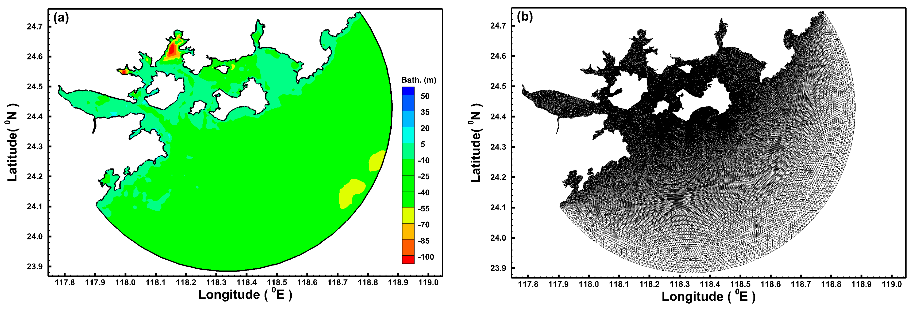
Figure 3.
Mode-data comparison for tide level at: (a) Suetau; and (b) Liaolowan.

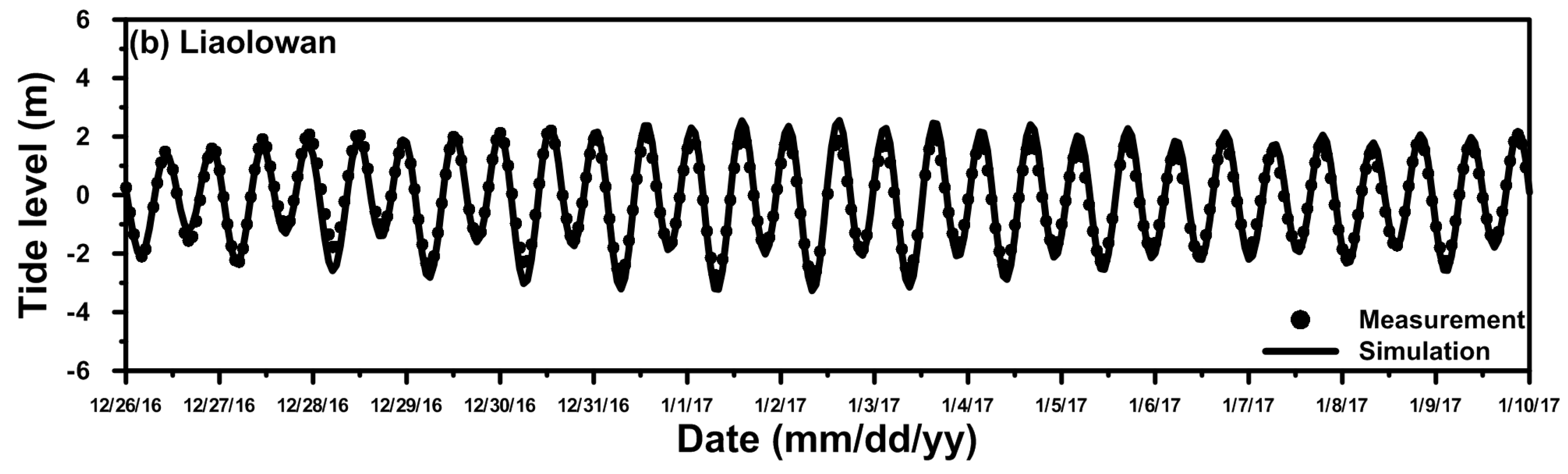
Figure 4.
Mode-data comparison for the depth-averaged current at Kinmen Buoy.

Figure 5.
(a) Distribution of the average current over a spring-neap cycle (i.e., 15 days) around Kinmen Island; and (b) turbine deployment site (gray box).
Figure 5.
(a) Distribution of the average current over a spring-neap cycle (i.e., 15 days) around Kinmen Island; and (b) turbine deployment site (gray box).
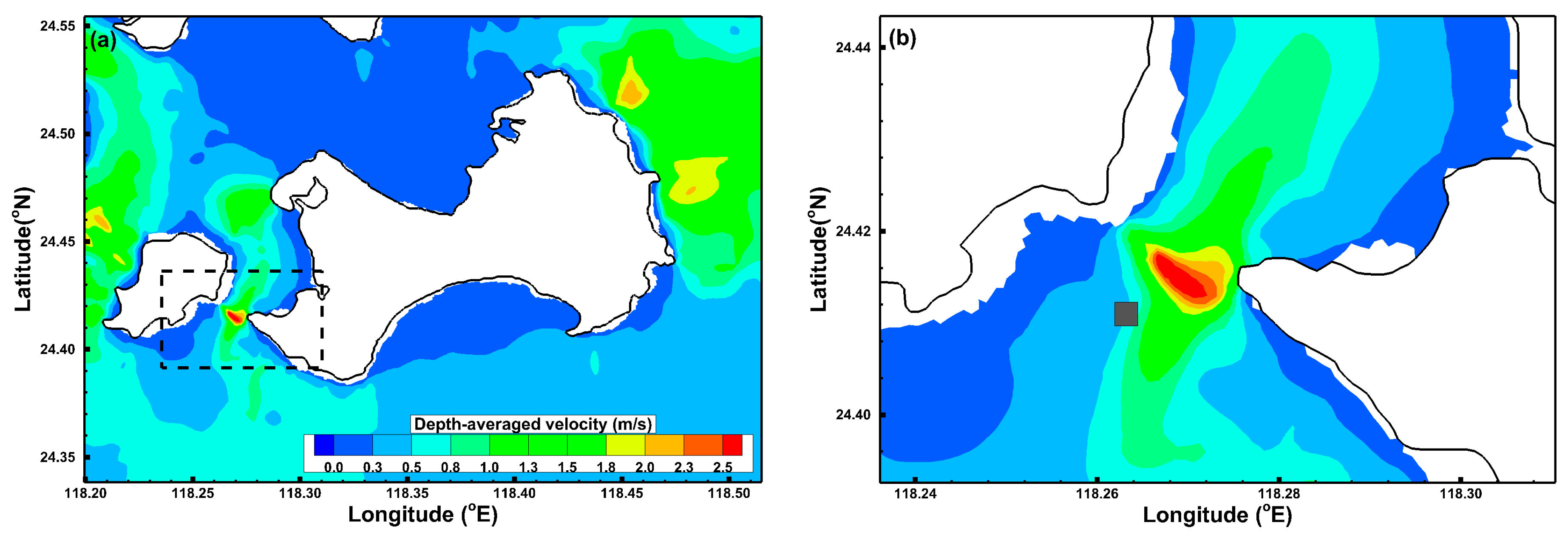
Figure 6.
Average TCP and its corresponding average current over a spring-neap cycle (i.e., 15 days) at the turbine deployment site.
Figure 6.
Average TCP and its corresponding average current over a spring-neap cycle (i.e., 15 days) at the turbine deployment site.
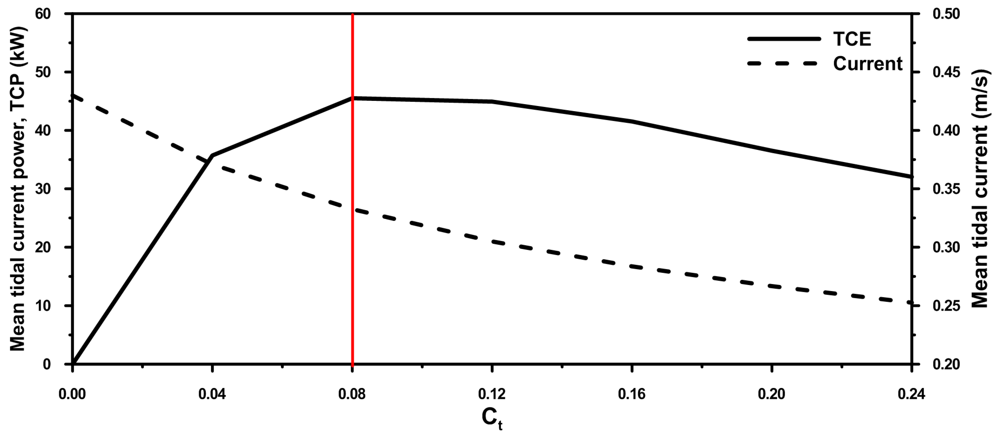
Figure 7.
Comparison of the time series of tide level between and at the turbine deployment site.
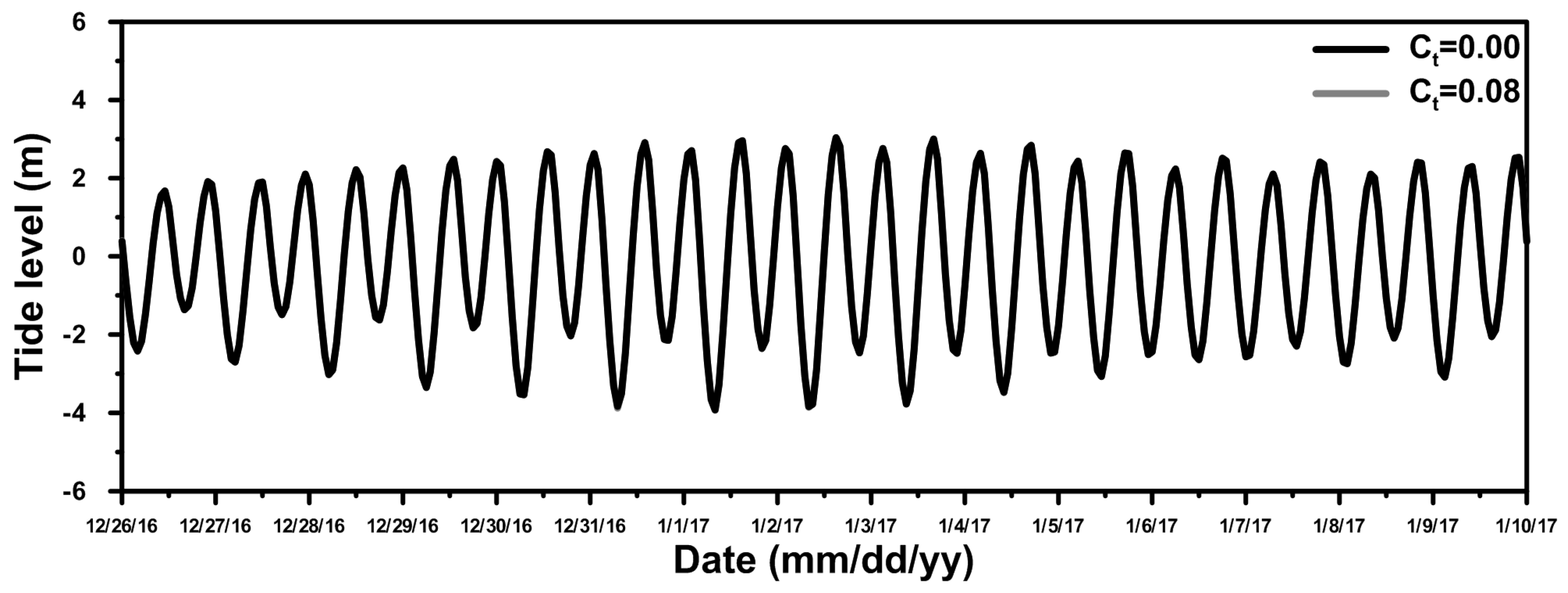
Figure 8.
(a) Spatial distribution of tide level (average tide level over a spring-neap cycle) differences between and around Kinmen waters; and (b) an enlarged view of the turbine site.
Figure 8.
(a) Spatial distribution of tide level (average tide level over a spring-neap cycle) differences between and around Kinmen waters; and (b) an enlarged view of the turbine site.

Figure 9.
Comparison time series of the current between and at the turbine deployment site.

Figure 10.
(a) Spatial distribution of current (average current over a spring-neap cycle) differences between and around Kinmen waters; and (b) an enlarged view of the turbine site.
Figure 10.
(a) Spatial distribution of current (average current over a spring-neap cycle) differences between and around Kinmen waters; and (b) an enlarged view of the turbine site.

Figure 11.
Average TCP over a spring-neap cycle (i.e., 15 days) for present-day sea level, sea-level rise (SLR) 0.25 m, SLR 0.5 m, SLR 0.75 m and SLR 1.0 m, and its corresponding .
Figure 11.
Average TCP over a spring-neap cycle (i.e., 15 days) for present-day sea level, sea-level rise (SLR) 0.25 m, SLR 0.5 m, SLR 0.75 m and SLR 1.0 m, and its corresponding .

Figure 12.
Average tidal current over a spring-neap cycle (i.e., 15 days) for present-day sea level, SLR 0.25 m, SLR 0.5 m, SLR 0.75 m and SLR 1.0 m, and its corresponding .
Figure 12.
Average tidal current over a spring-neap cycle (i.e., 15 days) for present-day sea level, SLR 0.25 m, SLR 0.5 m, SLR 0.75 m and SLR 1.0 m, and its corresponding .

Table 1.
Statistical errors of the model-data difference for tide levels and currents. MAPE: mean absolute percentage error.
Table 1.
Statistical errors of the model-data difference for tide levels and currents. MAPE: mean absolute percentage error.
| Variables | Suetau | Liaolowan | Kinmen Buoy | |||
|---|---|---|---|---|---|---|
| MAPE (%) | Skill | MAPE (%) | Skill | MAPE (%) | Skill | |
| Tide level | 17.68 | 0.93 | 15.14 | 0.93 | - | - |
| Current | - | - | - | - | 20.57 | 0.71 |
-: No data for comparison.
Table 2.
Amplitudes and phases of eight tidal constituents for Ct = 0.00 and Ct = 0.08 at the turbine site yielded by harmonic analysis.
Table 2.
Amplitudes and phases of eight tidal constituents for Ct = 0.00 and Ct = 0.08 at the turbine site yielded by harmonic analysis.
| Tidal Constituent | Amplitude (m) | Phase (o) | ||
|---|---|---|---|---|
| Ct = 0.00 | Ct = 0.08 | Ct = 0.00 | Ct = 0.08 | |
| M2 | 2.4714 | 2.4678 | 114.5893 | 114.8391 |
| S2 | 0.7518 | 0.7474 | 159.1727 | 159.7660 |
| N2 | 0.5004 | 0.4987 | 97.1582 | 97.4440 |
| K2 | 0.2300 | 0.2227 | 138.5008 | 139.2686 |
| K1 | 0.5387 | 0.5422 | 165.6684 | 165.0175 |
| O1 | 0.3885 | 0.3878 | 124.8016 | 124.7191 |
| P1 | 0.0765 | 0.0719 | 124.7396 | 125.4009 |
| Q1 | 0.0644 | 0.0634 | 102.3196 | 102.4989 |
© 2017 by the authors. Licensee MDPI, Basel, Switzerland. This article is an open access article distributed under the terms and conditions of the Creative Commons Attribution (CC BY) license (http://creativecommons.org/licenses/by/4.0/).
Share and Cite
MDPI and ACS Style
Chen, W.-B.; Chen, H.; Lin, L.-Y.; Yu, Y.-C. Tidal Current Power Resources and Influence of Sea-Level Rise in the Coastal Waters of Kinmen Island, Taiwan. Energies 2017, 10, 652. https://doi.org/10.3390/en10050652
AMA Style
Chen W-B, Chen H, Lin L-Y, Yu Y-C. Tidal Current Power Resources and Influence of Sea-Level Rise in the Coastal Waters of Kinmen Island, Taiwan. Energies. 2017; 10(5):652. https://doi.org/10.3390/en10050652
Chicago/Turabian StyleChen, Wei-Bo, Hongey Chen, Lee-Yaw Lin, and Yi-Chiang Yu. 2017. "Tidal Current Power Resources and Influence of Sea-Level Rise in the Coastal Waters of Kinmen Island, Taiwan" Energies 10, no. 5: 652. https://doi.org/10.3390/en10050652
Note that from the first issue of 2016, this journal uses article numbers instead of page numbers. See further details here.