
Bayesian Estimation of Remaining Useful Life for Wind Turbine Blades


Department of Civil Engineering, Aalborg University, Thomas Manns vej 23, DK-9220 Aalborg East, Denmark
*
Author to whom correspondence should be addressed.
Energies 2017, 10(5), 664; https://doi.org/10.3390/en10050664
Submission received: 20 February 2017
/
Revised: 4 May 2017
/
Accepted: 8 May 2017
/
Published: 10 May 2017
(This article belongs to the Special Issue Wind Turbine 2017)
Abstract
:To optimally plan maintenance of wind turbine blades, knowledge of the degradation processes and the remaining useful life is essential. In this paper, a method is proposed for calibration of a Markov deterioration model based on past inspection data for a range of blades, and updating of the model for a specific wind turbine blade, whenever information is available from inspections and/or condition monitoring. Dynamic Bayesian networks are used to obtain probabilities of inspection outcomes for a maximum likelihood estimation of the transition probabilities in the Markov model, and are used again when updating the model for a specific blade using observations. The method is illustrated using indicative data from a database containing data from inspections of wind turbine blades.
1. Introduction
Wind turbine blades are typically designed for a lifetime of 20 years. Nevertheless, variability in strength and loads and various incidents causing damage initiation, will cause some blades to fail earlier if the blades are not maintained. For offshore wind turbines, the costs associated with a major blade failure can be very large due to lost revenue and rent of expensive equipment, such as jack-up vessels, in addition to the cost of a new blade. Blades generally have a damage-tolerant design and will, therefore, not fail until they are severely damaged. Therefore, most blade failures can be avoided by repairing defects at an early state, before the defects become critical. Repairs of smaller defects can be made using rope access, and structural repairs can be made from a maintenance platform, which are both much cheaper than blade exchanges. To do so, defects must be detected by inspections or by condition monitoring at an early state. To adapt the optimal amount of condition monitoring, inspections, and maintenance, a risk-based approach can be used for operations and maintenance planning [1]. For this, probabilistic models are needed for prediction of the remaining useful life (RUL), and the models are updated using condition monitoring and inspection outcomes. This paper concerns the development of such a probabilistic deterioration model for wind turbine blades.
1.1. Failure Modes in Wind Turbine Blades
Wind turbine blades generally consist of a load carrying beam (the spar) enclosed by an aerodynamic shell. For modern wind turbines, both spar and shell are mainly made of composite materials, such as glass fiber laminates and, in the shell and webs of the spar, a sandwich structure is made with a lighter core material, e.g., balsa wood or polymer foams. The laminate consists of aligned fibers (glass or carbon fibers) embedded in a polymer matrix material (polyester, epoxy, or vinylester). Most blade manufacturers cast the shell in two parts, and use an adhesive to glue the parts together at the leading and trailing edge. The outer layer of the blade is a gel coat, protecting the blade structure from moist intrusion [2].
Wind turbine blades can suffer from various failure types. Distinction is made between blade failure (failure of the entire blade), and failure modes in the blade (macroscopic fault types in the blade). Failure modes include faults (e.g., cracking) in adhesive bonds, laminates, gel coats, and interfaces. Laminate failures can be visible cracks parallel, perpendicular or inclined with respect to the main fiber direction, or delamination cracks between plies (layers of fiber), or failure zones due to compression, tension, or shear loading. Cracks in the laminate or in the interfaces with laminate can occur with or without fiber bridging [2].
1.2. Deterioration Modelling for Wind Turbine Blades
Macroscopic growth of single cracks can be described theoretically using fracture mechanics. A crack will grow in a stable manner under a given load, if the energy release rate is below the fracture toughness of the material but above the threshold, where no crack growth occurs. The energy release rate is the sum of elastic strain energy and work done by external forces per unit of new crack area. The rate of growth can be described using Paris law:
where is the energy release rate range , and and are constants depending on material, mode mixity, temperature, stress ratio, and loading frequency [3]. For real detected cracks in wind turbines blades, there are many uncertainties involved in determining these. Even though this approach can, in principle, be used for the prediction of crack growth [4], the difficulties in obtaining the relevant parameters can be hard to overcome. An option is to obtain the parameters by calibration of a fracture mechanics (FM) model to give same reliability as a function of time as obtained using the stress-cycle (S-N) curve approach in design [5], as have been done for risk-based inspection (RBI) planning for fatigue cracks in oil and gas structures [6].
Alternatives to physical models, i.e., fracture mechanical modelling of single cracks for RUL prediction are methods based on data. Sikorska et al. [7] classified methods for RUL that rely on data as life expectancy models (stochastic or statistical), or artificial neural networks. Si et al. [8] considered statistical data-driven approaches for RUL estimation, and classified them based on the type of data: direct observation (e.g., crack size) or indirect observation (e.g., condition monitoring signal).
For composites, recent research has focused on RUL estimation based on online condition monitoring. For example, Peng et al. [9] used in situ stiffness measurements to estimate RUL of an open hole specimen using a Bayesian approach, and Eleftheroglou et al. [10] used acoustic emission data to update a semi-Markov model.
Modern offshore wind turbines typically have vibration-based condition monitoring (CM) systems installed on the drivetrain, able to detect incipient failures in, e.g., gearbox, main bearing, and generator. Even though several available sensor types can be applied for CM of blades, e.g., strain gauges, vibrational sensors, fiber optics, and acoustic emission sensors [11,12], the CM of blades is still in the developmental stage [13]. Laboratory testing [14] and prototype testing have been made, and studies of the rentability have been performed [15], but the long-term reliability and durability have yet to be tested, and only a few turbines have blade CM systems installed. Therefore, methods that rely solely on online CM will have limited applicability for blades of wind turbines currently installed, unless CM systems are installed later, which is more expensive compared to sensors embedded during production [11]. For currently-installed wind turbines, the blade health is, instead, examined using inspections, where access to the turbines is needed, in contrast to online CM.
Wind turbine blade inspections can be performed in several ways: from the ground/access platform, by drones (unmanned aerial vehicles), or as close-up manned inspections. Inspections performed from the ground can be made using binoculars, telephoto cameras, or computerized scan systems. Drones used for inspections can be equipped with both high definition (HD) video and infrared thermography video, to be able to detect some internal damages [16]. Close-up manned inspections can be made using rope access or from a suspended platform/basket, and can be visual in combination with thermography and nondestructive testing techniques, e.g., ultrasonic, shearography, and local resonance spectrography [11]. Generally, blade inspections cannot be considered to result in a direct estimate of the health of a blade, as not all defects are guaranteed to be detected. Generally, the larger the defect, the larger the probability of detection.
For wind turbine blades, a database for inspection data has been made, called Guide2defect [17], and is still under development. The database contains information from blade inspections on e.g., severity, type, and location of detected defects, and information on e.g., type, location, and age of the inspected wind turbines. The aim of this paper is to develop a procedure to use this type of inspection data for estimation of RUL, and to be able to update the RUL estimate for a specific wind turbine blade using inspection and/or CM data.
As inspections are uncertain, the model should allow to consider the probability of detection. A model type which allows for this is the hidden Markov model [8]. Florian and Sørensen [18] used blade inspections performed at one point in time for a fleet of turbines to obtain transition probabilities in a Markov model for the blade health, but the applied approach cannot be used when the turbines in the fleet were inspected at different points in time and several inspections of the same blade were performed, and they did not consider the probability of detection, when the transition probabilities were found. To consider multiple inspections of each blade, we apply the maximum likelihood method for the estimation of transition probabilities, and we apply dynamic Bayesian networks for modelling of a hidden Markov model for estimation of the likelihood of the data. For dynamic Bayesian networks, efficient methods are developed for probability updating, when the variables are discrete [19,20].
2. Dynamic Bayesian Network Model
Bayesian networks are graphical models consisting of nodes representing stochastic variables and directed links between the nodes, representing causal relationships. For a discrete model, each node has a discrete number of states, corresponding to the possible outcomes of the stochastic variable. If the stochastic variable is in fact continuous, it can be discretized such that each state represents an interval of values. To define the Bayesian network, the conditional probability distribution must be specified for each node conditioned on parent nodes (the nodes pointing towards a node). For a node with no parents, the marginal distribution is specified. The network can then be used for calculating the probability of each state for each of the nodes, and these probabilities can be updated, when any of the nodes are observed.
Dynamic Bayesian networks are especially appropriate for problems evolving with time like deterioration, as they consist of a sequence of time slices, each connected only to the previous and following time slice. Dynamic Bayesian networks can be applied for modelling of a Markov chain. For a Markov chain, the future is independent on the past, given the present, and it is modelled as a chain of nodes, each node pointing to the next. For RUL estimation, the nodes in the Markov chain can represent the deterioration state, e.g., damage size. When a Markov model is used, the RUL estimate only depends on the current deterioration state. For wind turbine blades, inspections are associated with uncertainty, and the current deterioration state is not directly observable. Therefore, a hidden Markov model is applied, as illustrated in Figure 1. The time slices generally contain two nodes: a node for the true deterioration state () with states, and a node for the observation of the deterioration state () with states.
For this model, time is discretized into a finite number of time steps, and the probabilities of transferring from each state to the following state within a time step are specified. In a Markov process where time is continuous, the time spent in each state follows an exponential distribution. When time is discretized, this becomes a geometric distribution. This assumption can be relaxed by using a semi-Markov model, where the time in each state does not have to be exponential distributed. To model this using a Bayesian network, each ‘physical’ state is divided into several virtual states, to obtain another sojourn time distribution for the physical state, and the time spent in each virtual state is still exponentially distributed [21]. Dynamic Bayesian networks can also be applied for deterioration modelling based on physical models as shown in Equation (1) [22].
The network in Figure 1 is specified in terms of three probability distributions:
- : prior probability distribution for the initial deterioration state ( vector).
- : conditional probability distribution for the deterioration state in time step given the deterioration state in time step ( matrix).
- : conditional probability distribution for the observation of the deterioration state in time step given the deterioration state in time step ( matrix).
When these three probability distributions are specified, the Bayesian network model can be used for computing the marginal distribution of and for each time step. When no observations have been made, this can be done using forward computing. Sequentially, starting at , the marginal distribution for is found by elementwise multiplication of and to obtain the joint distribution , and then marginalizing out by summation:
When the probability distributions are given as matrices and vectors, this operation corresponds to matrix multiplication. In the same way, the marginal distribution for can be obtained:
When any of the nodes are observed, this affects how the computations are performed. The marginal distribution can be updated, when is observed by applying Bayes rule. The marginal distribution for given the observation is:
where “∝” means “proportional to”. After elementwise multiplication, the distribution is scaled to sum to one.
The task of computing the distribution for time steps , when observations are received for nodes up to , is so-called filtering. It is performed by applying Equations (2) and (4) sequentially. The task of computing the distribution for time steps , when observations are received for nodes up to , is so-called prediction. This is simply performed by applying Equation (2) sequentially.
2.1. Model Specification
To obtain the probability distributions , , and , inspection data in the Guide2defect database is considered for illustration. The database contains an entry for each defect detected during an inspection. For inspections of blades without the detection of any defects, an entry for “no detected defects” is made. The defects are classified based on the type, and categorized based on the severity of the defect. Categorizations similar to the one applied in the database are commonly used in the wind turbine inspection industry [23]. For cracks in the laminate, the categorization is performed based on the size of the crack. For each crack present in the blade, there are seven possible outcomes for an inspection, as shown in Table 1, as these are the categories used in the database. These seven possible outcomes are the states for the node , if the variable represents the size of a specific crack.
If we are interested in a model for the overall health of the blade for the estimation of the RUL, it is not enough to consider each crack separately. Instead, a model is made where the variable represents the overall health of the blade. We assume that the largest crack dominates the repair costs and the probability of failure, and let the variable represent the size of the largest crack in the blade. If the deterioration model calibration is performed based on observations of the largest crack in the blade, the model considers both the possibility that the largest detected crack grows, and the possibility that a smaller crack grows to become the largest. We hereby consider all cracks as belonging to the same population.
The states for the node for the true damage size () must be related to the states of the node for the observed damage size () through the inspection model. It is natural to choose the same states for as for , except for the first state, which should be “no crack initiated” instead of “no detection”.
Adding more sub-states within each observed state can make it possible to model a non-exponential sojourn time. If a physical model was available or each blade was inspected many times, it would be relevant to study the effect of adding more states. However, in the available data, each blade is only inspected one or a few times, and a more accurate estimate of the sojourn time distribution cannot be made. We, therefore, use the same number of states for the deterioration model as for the inspection model, and assume that it is not possible for a crack to grow more than one state during each time step. Then, the conditional probability distribution is defined in terms of six transition probabilities to :
If we assume that no cracks are present in the first time step, the distribution for the initial crack size is:
The inspection model should reflect the reliability of the inspection method being used. For the current version of the database, the inspection method is not specified. We assume that all inspections are visual inspections performed using rope access, that detected cracks are classified correctly, and that no false detections occur. Then, the inspection model is defined based on the probability of detection for each crack size, to :
2.2. Calibration of Markov Deterioration Model Using Inspection Data
Several methods exist for the assessment of probability distributions in a Bayesian network model [7,19]. Here, we apply the maximum likelihood method for estimation of the transition probabilities. In the maximum likelihood method, the transition probabilities are found such that the probability of getting the observed dataset is maximized. To avoid numerical underflow, the logarithm of the product of the probabilities is taken instead, yielding the objective function:
where is the probability of data point for a given set of transition probabilities . Each data point contains information on maximum observed crack size (), age at the time step of inspection (), and blade identification number (). The age () should be given as the number of whole time steps, e.g., months. The dataset is assumed to contain information from one or more inspections for several identical wind turbine blades.
For blades only inspected once, the probability is obtained by applying Equation (2) sequentially for , and then applying Equation (3) for , to get the marginal distribution . The probability of data point is then .
For blades inspected several times, the observations are not independent, and the joint probability of all data points is found using Bayes rules to obtain conditional probabilities. For example, for two observations and of the same blade, the joint probability can be found by multiplication of the probability of the first data point and the probability of the second data point given the first data point:
The probability of the first data point is obtained in the same way, as for blades only inspected once. Then, to obtain the conditional probability of the second data point given the first, Equation (4) is applied for the first data point for . Then Equation (2) is applied sequentially for and, finally, Equation (3) is applied for such that the probability can be retrieved.
The most likely set of transition probabilities is found by solving the maximization problem using a built-in solver for non-linear constrained optimization in MATLAB [24]. The objective function was given in Equation (8), and the constraints for the transition probabilities are the general bounds for probabilities; zero and one.
3. Example
In this example, preliminary data from the database Guide2defect [17] is used for demonstration of the method. Due to confidentiality, the raw data used in the example is not publicly available. To ensure homogeneity in the data, one specific wind turbine model is selected, and all data for this model is extracted. For each blade inspection, the following information is identified: the category of the largest detected crack (or the information that no cracks have been detected), the age of the blade at the time of inspection, and the identification number of the blade. The division of the observations on crack category is shown in Table 3.
In several cases, the same blade has been inspected several times. The method presented in Section 2.2 assumes that the blade has not been repaired between inspections, but in reality, blades will often be repaired after detection of cracks, especially larger cracks. The present version of the database does not contain information of repairs and, therefore, assumptions must be made concerning repairs. If the same blade is inspected several times, and the size of the largest detected crack declines between inspections, it is most likely, that a repair has been made. If the size of the largest crack stays the same or increases, it could be the same crack, if it has not been repaired, or a new crack both if it has or has not been repaired. To identify whether previously detected cracks are still present, the following information on the type and location of the detected cracks is considered:
- Reference number (contains blade ID);
- Defect code (type of defect);
- Section (approximate location on blade in longitudinal direction);
- Outside profile position (location on blade in transverse direction);
- Profile side (suction side, pressure side, leading edge, trailing edge); and
- Defect “radius” (distance from blade root to defect).
The defect radius is a measurement and is, therefore, somewhat uncertain. Two observations are assumed to be observations of the same crack, if the difference in defect radius is less than one meter, and if all other information on location and type is equal. With this information, each crack can be assigned a crack ID number and can be tracked. If the largest crack detected at an inspection is not found in a later inspection, it is assumed to be repaired, and the data from after the repair is discarded. The damage categories for the remaining observations are shown in Table 4.
Based on the dataset summarized in Table 4 and the method outlined in Section 2, the estimates of the transition probabilities in the Markov model are found and are shown together with the mean sojourn time in each state in Table 5. The time step used in the model is one month.
3.1. Estimation of RUL—Remaining Useful Life
Defects of both category 5 and 6 are classified as critical, and we assume that a blade exchange is necessary for both types of defects. Therefore, the remaining useful life is assumed to end when the blade enters state 5, even though it is still able to operate, but at a high risk of catastrophic failure.
If the current state is known, the mean RUL can be found directly by addition of the mean sojourn times from the current state. For a blade in state 0, the mean RUL is 183.1 months (15.3 years). If the useful life was assumed to end when the blade enters state 6, mean RUL is 222.9 months (18.6 years).
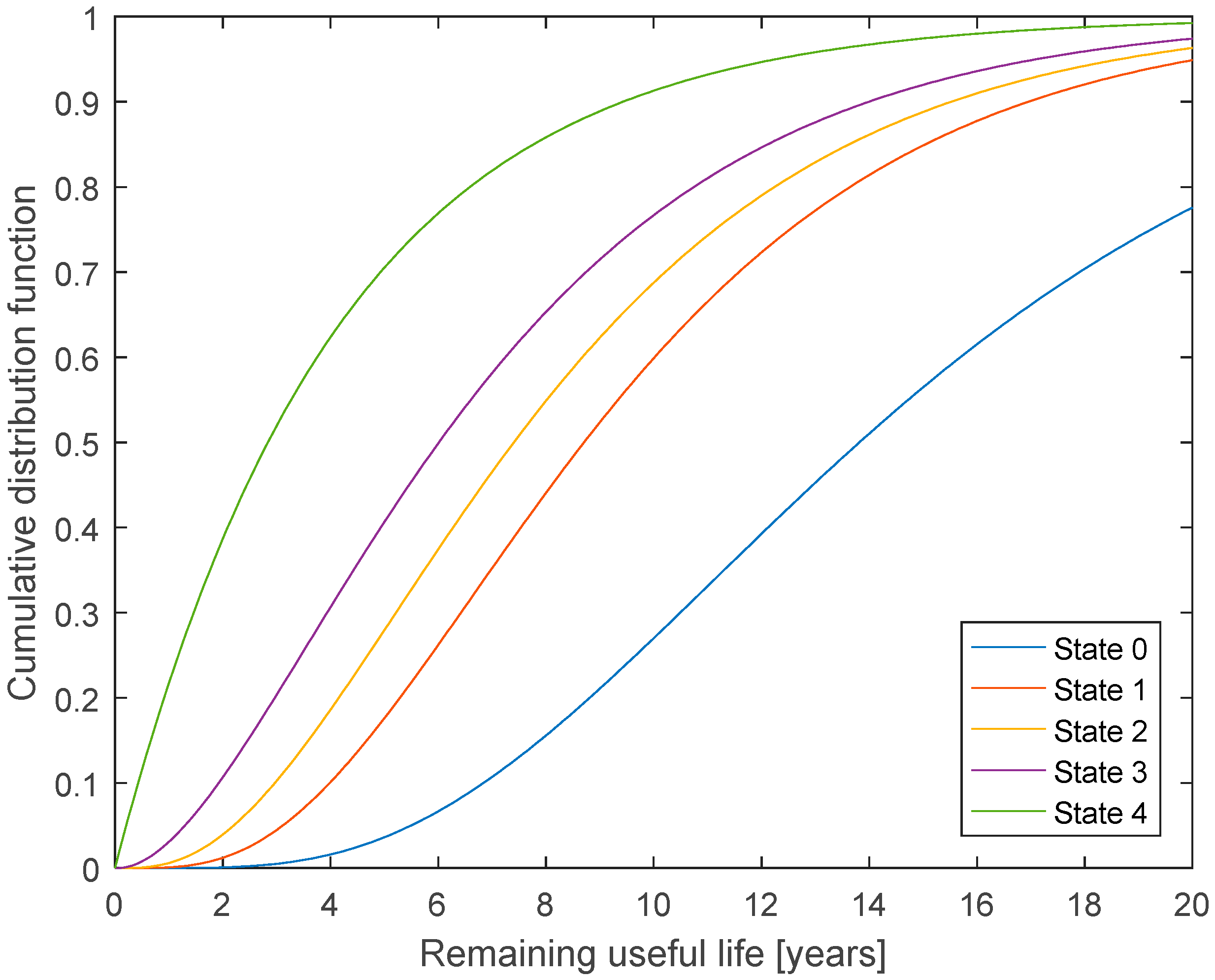
As there is large uncertainty on the RUL, the distribution for RUL is of interest. The Bayesian network model can be used for estimation of the probability distribution for RUL. If the current state is known (or the current distribution for the deterioration state is known), this information can be used as initial deterioration state , and Equation (2) can be used to find the distribution for future deterioration states. For each time step, the value of the cumulative distribution function can be found as the sum of the probability for state 5 and 6. Figure 2 shows the resulting cumulative distribution function for RUL, when the current state is known.
3.2. Updating Using Inspections
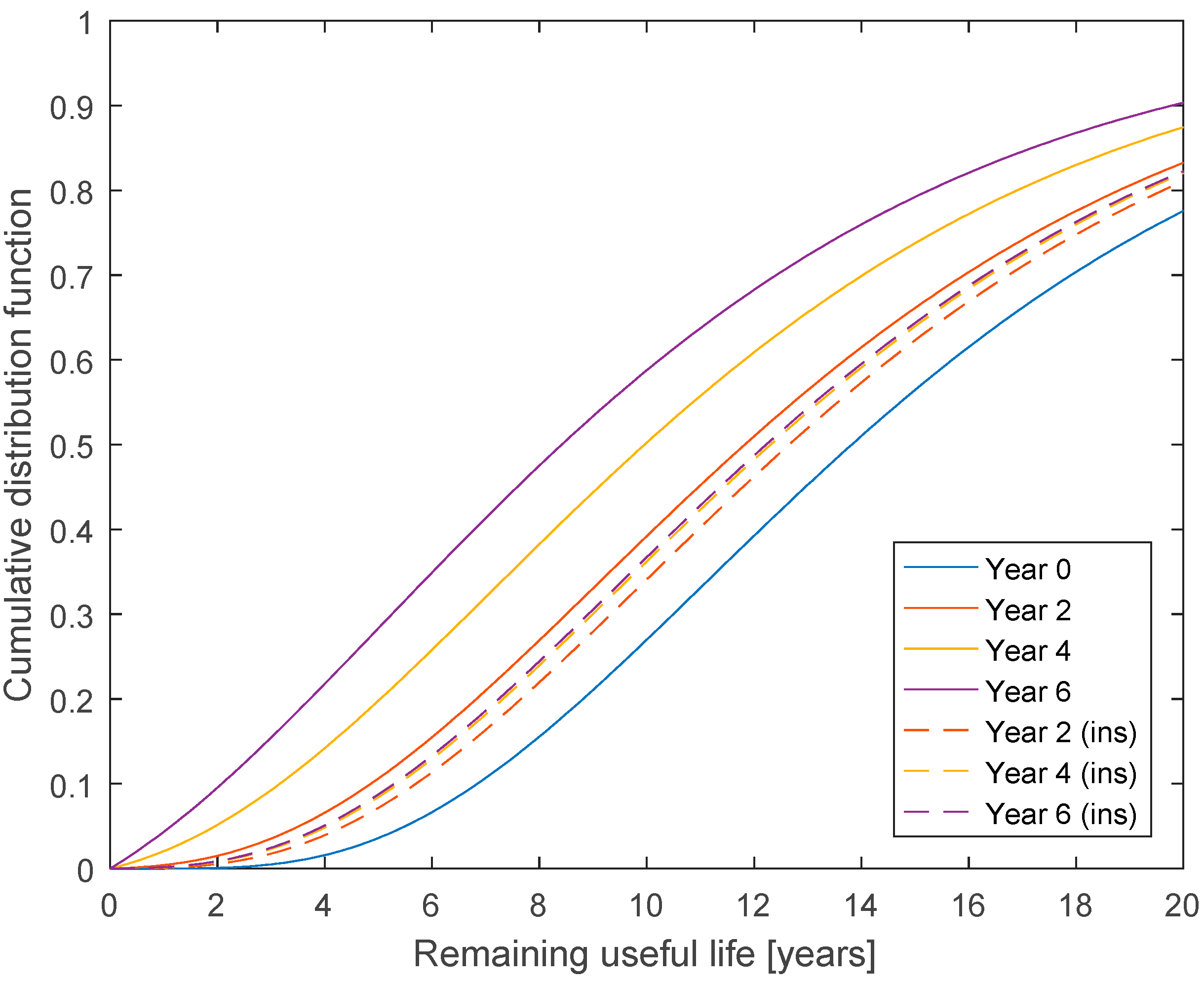
The Bayesian network model can also be used for estimation of RUL, when the current state is not known for certain. When inspection data is available, Bayesian updating can be performed using Equation (4) for time steps with inspections. A similar updating can be performed, if it is known that the useful life has not yet ended. Figure 3 shows the distribution for RUL at year 0, and at year 2, 4, and 6 if it is known that the lifetime has not yet ended, and if annual inspections are made, and no cracks are detected during the inspections.
The updating of the curves depends on the probability of detection for each deterioration state. If a less reliable inspection technique was used, the probability of detection would be reduced. If the values for states 1 to 5 was reduced to 20%, 40%, 80%, 90%, and 95%, respectively, and annual inspections were still made, the estimated RUL would be reduced, as shown in Figure 4.
3.3. Updating Using Condition Monitoring
Compared to inspections, CM has the advantage that information is continuously received without need to access the turbines. If a CM system is installed for health monitoring of the blades, the information from it can be used for updating of the RUL in the same way as inspection information under the following conditions: (1) the model is updated once every time step using a statistical value of the processed signal, e.g., mean or maximum value; (2) the observations used for updating are independent given the damage size. A model for the reliability of the CM method is needed, and should be derived based on information of the actual CM system and the statistics used for updating.
An example of a model with four possible states is shown in Table 6. The values are fictive, but represent a system, where the probability of detection per time step is lower than for a visual inspection, and where two alarm levels have been set. The system is assumed always to detect failures, defined as cracks larger than 3 meters (category 6). Cracks less than 50 mm (category 1) are never detected, and for cracks between 50 mm and 3 m, the probability of detection increases with size, and the probability of high alarm compared to low alarm increases with size.
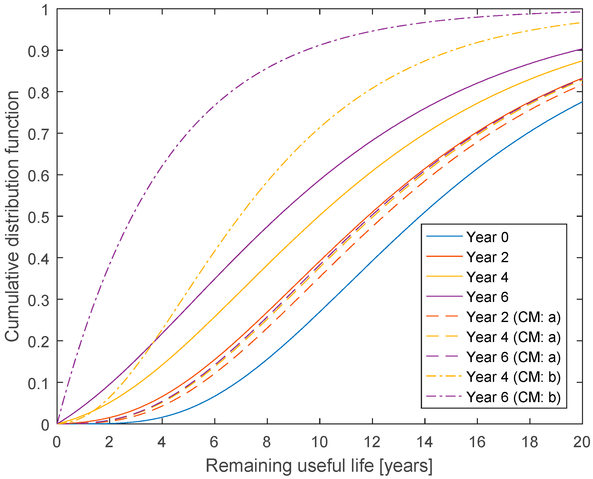
Figure 5 shows two examples of how the RUL estimate is updated using information from CM, together with the case, where RUL is just updated using the information that the useful life has not yet ended. In the first example (CM: a in Figure 5), the CM system is assumed to have the outcome “no detection” in all time steps, until the RUL estimate is made. In the second example (CM: b in Figure 5), the CM signal is assumed to change to “low alarm” after four years. With a CM system with “no detection”, the curve almost stops to move after four years. However, when the first “low alarm” is received after four years, the curve moves to a much lower estimate of RUL, and when “low alarm” is continuously received from the fourth to the sixth year, the curve has moved further. The RUL estimates updated using CM can be used as basis for decisions on inspections using a risk-based approach [1]. Decision rules for inspections can for example be based on the probability of failure within a reference period or the mean (or median) remaining useful life, and the optimal decision rule can be determined as the one resulting in the lowest expected lifetime costs.
4. Conclusions and Discussion
In this paper, a dynamic Bayesian network approach was applied for the estimation of the remaining useful life for wind turbine blades. The maximum likelihood method was applied successfully for the estimation of transition probabilities for a hidden Markov model. Generally, the maximum likelihood method is suitable for estimation of conditional probability distributions for complete dataset, and may not succeed in finding a solution for incomplete data. However, for this application it was assumed, that no states could be skipped, and the conditional probability distribution was specified only in terms of six transition probabilities. For less constrained models, other approaches can be applied for the estimation of probabilities, e.g., the expectation maximization (EM) algorithm [19]. This could be relevant for other wind turbine components, where CM is already implemented, and where CM data is available for the development of deterioration models.
The found transition probabilities were largest for transition from states 1 and 2. The reason for this can be seen in the inspection data, where only few cracks in categories 1 and 2 was found compared to states 3 and 4. Therefore, on average, each crack can only have this size for a short time, otherwise more cracks of these sizes would have been found. However, the transition probabilities also depend on the assumed inspection model. If the probability of detection values were decreased for states 1 and 2, which could also explain the lack of observations, and the resulting transition probabilities for states 1 and 2 would be smaller. However, the other transition probabilities would also be adjusted, such that the effect on the mean RUL for state 0 would be limited.
After the transition probabilities are found, the Bayesian network model can be used for the estimation of RUL, and can be updated using observations from inspections or CM. If no observations were made, the RUL gradually decreased with time. However, when inspections were made, and nothing was detected, the RUL estimate stagnated. It stagnated at a lower RUL, if a less reliable inspection technique was used. Condition monitoring also provided efficient stagnation of the RUL estimate, when nothing was detected, even though the reliability of CM was assumed to be lower than inspections. On the other hand, CM outcomes were achieved in all time steps, not only annually as was assumed for inspections. It should be noted that the observations were assumed to be independent, given the model. In reality, it would be fairer to account for some dependence between CM outcomes in different time steps, as the location and type of crack would affect the probability of detection. Ignoring a correlation, which is, in fact, present could lead to RUL estimates that are too optimistic. The correlation between observations can be included by adding a joint parent node for the nodes for CM outcomes and is an important topic for future research.
Acknowledgments
The research leading to these results has been conducted under the LEANWIND project, which has received funding from the European Union Seventh Framework Programme under the agreement SCP2-GA-2013-614020. The funds cover the costs to publish in open access.
Author Contributions
The main idea for the paper was proposed by John D. Sørensen, and Jannie S. Nielsen developed the models and wrote the first draft of the paper. John D. Sørensen thoroughly reviewed the paper.
Conflicts of Interest
The authors declare no conflict of interest. The founding sponsors had no role in the design of the study; in the collection, analyses, or interpretation of data; in the writing of the manuscript, and in the decision to publish the results.
References
- Nielsen, J.S.; Sørensen, J.D. Methods for risk-based planning of O&M of wind turbines. Energies 2014, 7, 6645–6664. [Google Scholar]
- Sørensen, B.F.; Holmes, J.W.; Brøndsted, P.; Branner, K. Blade materials, testing methods and structural design. In Wind Power Generation and Wind Turbine Design; Tong, W., Ed.; WIT Press: Southampton, UK, 2010; pp. 417–466. [Google Scholar]
- Kenane, M.; Benzeggagh, M.L. Mixed-mode delamination fracture toughness of unidirectional glass/epoxy composites under fatigue loading. Compos. Sci. Technol. 1997, 57, 597–605. [Google Scholar] [CrossRef]
- McGugan, M.; Pereira, G.; Sørensen, B.F.; Toftegaard, H.; Branner, K. Damage tolerance and structural monitoring for wind turbine blades. Philos. Trans. R. Soc. A 2015, 373. [Google Scholar] [CrossRef] [PubMed]
- DNV GL. DNV GL Standard, Rotor Blades for Wind Turbines; DNVGL-ST-0376; DNV GL: Oslo, Norway, 2015. [Google Scholar]
- Straub, D. Generic Approaches to Risk Based Inspection Planning for Steel Structures. Ph.D. Thesis, Swiss Federal Institute of Technology, ETH Zurich, Zurich, Switzerland, 2004. [Google Scholar]
- Sikorska, J.Z.; Hodkiewicz, M.; Ma, L. Prognostic modelling options for remaining useful life estimation by industry. Mech. Syst. Signal Process. 2011, 25, 1803–1836. [Google Scholar] [CrossRef]
- Si, X.-S.; Wang, W.; Hu, C.-H.; Zhou, D.-H. Remaining useful life estimation—A review on the statistical data driven approaches. Eur. J. Oper. Res. 2011, 213, 1–14. [Google Scholar] [CrossRef]
- Peng, T.; Liu, Y.; Saxena, A.; Goebel, K. In-situ fatigue life prognosis for composite laminates based on stiffness degradation. Compos. Struct. 2015, 132, 155–165. [Google Scholar] [CrossRef]
- Eleftheroglou, N.; Theodoros, L. Fatigue damage diagnostics and prognostics of composites utilizing structural health monitoring data and stochastic processes. Struct. Health Monit. 2016, 15, 473–488. [Google Scholar] [CrossRef]
- Katnam, K.B.; Comer, A.J.; Roy, D.; da Silva, L.F.M.; Young, T.M. Composite Repair in Wind Turbine Blades: An Overview. J. Adhes. 2015, 91, 113–139. [Google Scholar] [CrossRef]
- Li., D.; Ho, D.M.; Song, G.; Ren, L.; Li, H. A review of damage detection methods for wind turbine blades. Smart Mater. Struct. 2015, 24. [Google Scholar] [CrossRef]
- Coronado, D.; Fischer, K. Condition Monitoring of Wind Turbines: State of the Art, User Experience and Recommendations; Project Report; Fraunhofer IWES: Freiburg, Germany, 2015. [Google Scholar]
- Tcherniak, D.; Mølgaard, L.L. Vibration-based SHM System: Application to Wind Turbine Blades. J. Phys. Conf. Ser. 2015, 628. [Google Scholar] [CrossRef]
- May, A.; McMillan, D.; Thöns, S. Economic analysis of condition monitoring systems for offshore wind turbine sub-systems. IET Renew. Power Gener. 2015, 9, 900–907. [Google Scholar] [CrossRef]
- Calleguillos, C.; Zorrilla, A.; Jimenez, A.; Diaz, L.; Montiano, Á.L.; Barroso, M.; Viguria, A.; Lasagni, F. Thermographic non-destructive inspection of wind turbine blades using unmanned aerial systems. Plast. Rubber Compos. 2015, 44, 98–103. [Google Scholar] [CrossRef]
- Guide2defect. Available online: http://guide2defect.com/ (accessed on 16 January 2017).
- Florian, M.; Sørensen, J.D. Case study for impact of D-string® on levelized cost of energy for offshore wind turbine blades. Int. J. Offshore Polar 2017, 27, 63–69. [Google Scholar] [CrossRef]
- Jensen, F.V.; Nielsen, T.D. Bayesian Networks and Decision Graphs, 2nd ed.; Springer: New York, NY, USA, 2007. [Google Scholar]
- Murphy, K. Dynamic Bayesian Networks: Representation, Inference and Learning. Ph.D. Thesis, University of California, Berkeley, CA, USA, 2002. [Google Scholar]
- Welte, T.M. A rule-based approach for establishing states in a Markov process applied to maintenance modelling. Proc. IMechE 2009, 223. [Google Scholar] [CrossRef]
- Straub, D. Stochastic modelling of deterioration processes through dynamic Bayesian networks. J. Eng. Mech. ASCE 2009, 135, 1089–1099. [Google Scholar] [CrossRef]
- Meneses, R. How to Create the Optimal Maintenance and Inspection Strategy to minimize OPEX; Iberwind, from Blade Inspection Damage & Repair workshop. Windpower Monthly, 10 October 2016. [Google Scholar]
- MATLAB Release 2016a; The MathWorks, Inc.: Natick, MA, USA.
Figure 1.
Hidden Markov model.
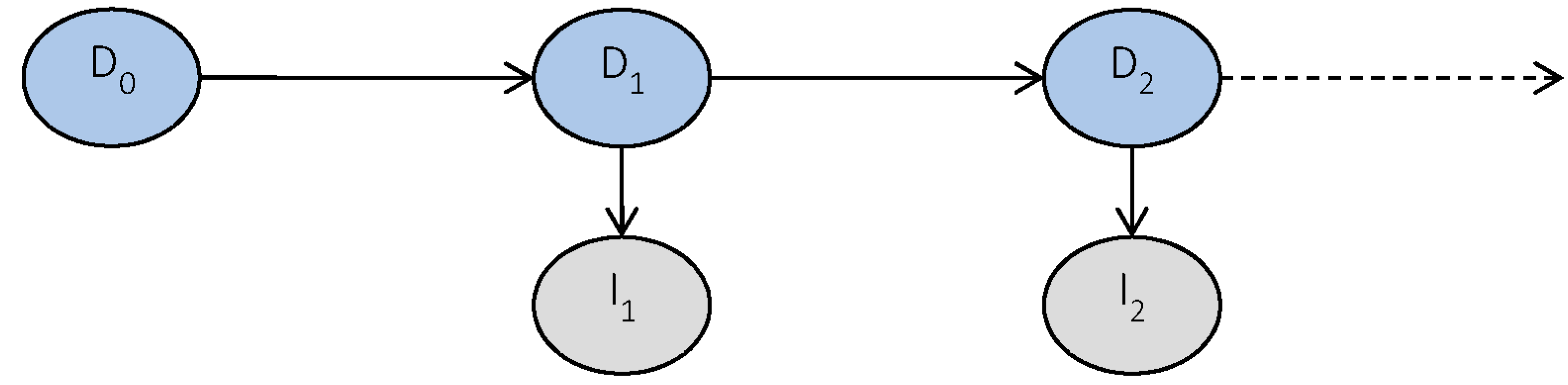
Figure 2.
Cumulative distribution function for remaining useful life for current state zero to four.
Figure 2.
Cumulative distribution function for remaining useful life for current state zero to four.

Figure 3.
Cumulative distribution function for the remaining useful life 0, 2, 4, and 6 years into the lifetime. The dashed lines are for after annual inspections with no detected cracks.
Figure 3.
Cumulative distribution function for the remaining useful life 0, 2, 4, and 6 years into the lifetime. The dashed lines are for after annual inspections with no detected cracks.
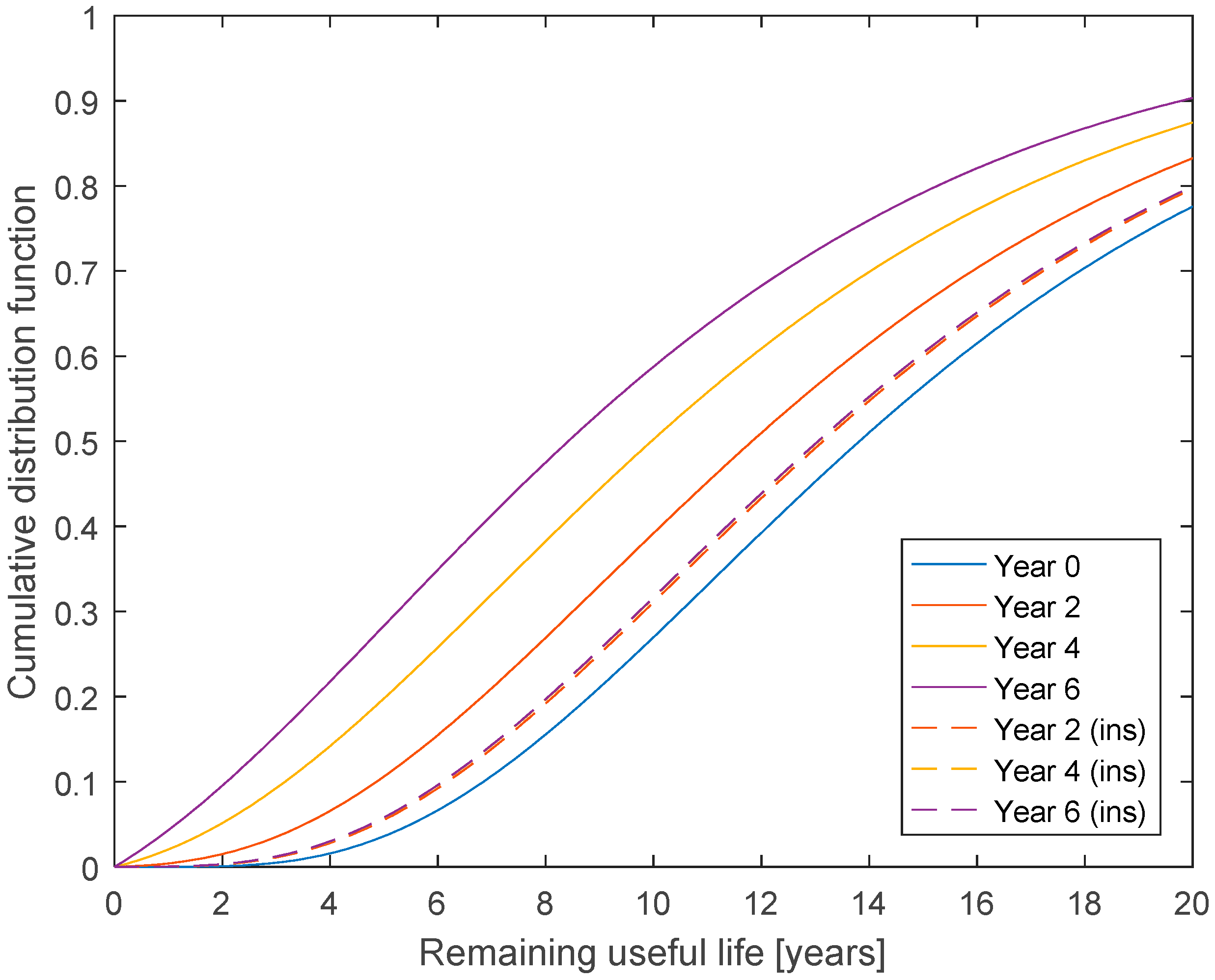
Figure 4.
Cumulative distribution function for the remaining useful life 0, 2, 4, and 6 years into the lifetime. The dashed lines are for after annual inspections with no detected cracks with reduced PoD values.
Figure 4.
Cumulative distribution function for the remaining useful life 0, 2, 4, and 6 years into the lifetime. The dashed lines are for after annual inspections with no detected cracks with reduced PoD values.

Figure 5.
Cumulative distribution function for the remaining useful life 0, 2, 4, and 6 years into the lifetime. The dashed lines (CM: a) are for CM system with no detection, and the dash-dot lines (CM: b) are for CM with no alarm until four years into the lifetime, and for low alarm after four years.

Table 1.
States for .
| State for I | Category | Observed Crack Size |
|---|---|---|
| 0 | No detection | - |
| 1 | Cosmetic | 0–50 mm |
| 2 | Damage, below wear and tear | 50–200 mm |
| 3 | Damage, above wear and tear | 200–500 mm |
| 4 | Serious damage | 500–1000 mm |
| 5 | Critical damage | 1000–3000 mm |
| 6 | Critical damage | >3000 mm |
Table 2.
Probability of detection (PoD) for each defect size.
| State for D | Crack Size | PoD |
|---|---|---|
| 0 | - | 0 |
| 1 | 0–50 mm | 40% |
| 2 | 50–200 mm | 80% |
| 3 | 200–500 mm | 90% |
| 4 | 500–1000 mm | 95% |
| 5 | 1000–3000 mm | 98% |
| 6 | >3000 mm | 100% |
Table 3.
Number of cracks of each category for largest detected crack from each inspection.
| State for I | Category | Number of Observations |
|---|---|---|
| 0 | No detection | 124 |
| 1 | Cosmetic | 14 |
| 2 | Damage, below wear and tear | 34 |
| 3 | Damage, above wear and tear | 76 |
| 4 | Serious damage | 59 |
| 5 | Critical damage | 29 |
| 6 | Critical damage | 18 |
Table 4.
Number of cracks of each category for largest detected crack from each inspection after discarding data after assumed repairs.
Table 4.
Number of cracks of each category for largest detected crack from each inspection after discarding data after assumed repairs.
| State for I | Category | Number of Observations |
|---|---|---|
| 0 | No detection | 103 |
| 1 | Cosmetic | 12 |
| 2 | Damage, below wear and tear | 25 |
| 3 | Damage, above wear and tear | 67 |
| 4 | Serious damage | 56 |
| 5 | Critical damage | 27 |
| 6 | Critical damage | 18 |
Table 5.
Transition probabilities and mean sojourn time for each state.
| State for D | Transition Probability P | Mean Sojourn Time [Months] |
|---|---|---|
| 0 | 0.0154 | 65.1 |
| 1 | 0.0663 | 15.1 |
| 2 | 0.0626 | 16.0 |
| 3 | 0.0269 | 37.2 |
| 4 | 0.0201 | 49.7 |
| 5 | 0.0252 | 39.8 |
| 6 | - | - |
Table 6.
Condition monitoring model.
| State for I | Crack Size | No Detection | Low Alarm | High Alarm | Failure |
|---|---|---|---|---|---|
| 0 | - | 100% | 0 | 0 | 0 |
| 1 | 0–50 mm | 100% | 0 | 0 | 0 |
| 2 | 50–200 mm | 90% | 10% × 80% | 10% × 20% | 0 |
| 3 | 200–500 mm | 80% | 20% × 60% | 20% × 40% | 0 |
| 4 | 500–1000 mm | 60% | 40% × 40% | 40% × 60% | 0 |
| 5 | 1000–3000 mm | 20% | 80% × 20% | 80% × 80% | 0 |
| 6 | >3000 mm | 0 | 0 | 0 | 100% |
© 2017 by the authors. Licensee MDPI, Basel, Switzerland. This article is an open access article distributed under the terms and conditions of the Creative Commons Attribution (CC BY) license (http://creativecommons.org/licenses/by/4.0/).
Share and Cite
MDPI and ACS Style
Nielsen, J.S.; Sørensen, J.D. Bayesian Estimation of Remaining Useful Life for Wind Turbine Blades. Energies 2017, 10, 664. https://doi.org/10.3390/en10050664
AMA Style
Nielsen JS, Sørensen JD. Bayesian Estimation of Remaining Useful Life for Wind Turbine Blades. Energies. 2017; 10(5):664. https://doi.org/10.3390/en10050664
Chicago/Turabian StyleNielsen, Jannie S., and John D. Sørensen. 2017. "Bayesian Estimation of Remaining Useful Life for Wind Turbine Blades" Energies 10, no. 5: 664. https://doi.org/10.3390/en10050664
Note that from the first issue of 2016, this journal uses article numbers instead of page numbers. See further details here.