
The Optimal Road Grade Design for Minimizing Ground Vehicle Energy Consumption


1
School of Electro-Mechanical Engineering, Xidian University, Xi’an 710071, China
2
Key Laboratory of Electronic Equipment Structure Design, Ministry of Education, Xi’an 710071, China
3
Department of Machine Design, KTH Royal Institute of Technology, Stockholm SE-10044, Sweden
4
Institute of Systems Engineering, Macau University of Science and Technology, Taipa 999078, Macau
*
Authors to whom correspondence should be addressed.
Energies 2017, 10(5), 700; https://doi.org/10.3390/en10050700
Submission received: 7 April 2017
/
Revised: 9 May 2017
/
Accepted: 10 May 2017
/
Published: 16 May 2017
(This article belongs to the Special Issue Methods to Improve Energy Use in Road Vehicles)
Abstract
:Reducing energy consumption of ground vehicles is a paramount pursuit in academia and industry. Even though the road infrastructural has a significant influence on vehicular fuel consumption, the majority of the R&D efforts are dedicated to improving vehicles. Little investigation has been made in the optimal design of the road infrastructure to minimize the total fuel consumption of all vehicles running on it. This paper focuses on this overlooked design problem and the design parameters of the optimal road infrastructure is the profile of road grade angle between two fixed points. We assume that all vehicles on the road follow a given acceleration profile between the two given points. The mean value of the energy consumptions of all vehicles running on the road is defined as the objective function. The optimization problem is solved both analytically by Pontryagin’s minimum principle and numerically by dynamic programming. The two solutions agree well. A large number of Monte Carlo simulations show that the vehicles driving on the road with the optimal road grade consume up to 31.7% less energy than on a flat road. Finally, a rough cost analysis justifies the economic advantage of building the optimal road profile.
1. Introduction
With the rapid increase of the number of automobiles, worldwide energy consumption and greenhouse gas emissions have increased greatly. It is a challenge for the automotive industry to reduce energy consumption and carbon emissions. For this purpose, academia and industry have paid much attention to the energy consumption minimization of ground vehicles. For example, many solutions to alternative powertrains have been proposed, including hybrid electric vehicles (powered by an internal combustion engine and at least one electric motor) [1,2,3,4,5], full electric vehicles [6,7,8] and fuelcell vehicles [9,10]. Hybrid powertrains already became an affordable and popular approach to higher fuel efficiency and there are many successful products from Toyota, Honda, Volvo, BYD and so on. In addition to improving the energy efficiency of powertrains, the auxiliary systems, such as the power-assisted steering and brake and thermal management system, are also optimized for better energy efficiency [11,12,13,14,15].
Another significant way for reducing fuel consumption is the optimal energy management control strategies [16]. There are plentiful publications on this topic using different optimization approaches, e.g., dynamic programming [3,17,18], convex optimization [13], Pontryagin’s minimum principle [19] and equivalent fuel consumption minimization strategy [20]. These have been applied to achieve fuel optimal driving in conventional cars and trucks [21], fuelcell cars [8] and electric cars [7]. Model predictive control recently becomes popular for energy management control of ground vehicles when future road condition is predictable [22,23].
Ecological cruise control, namely eco-driving, is an emerging technique for reducing fuel consumption through varying vehicle speed according to road grade angle [24]. The road grade is the angle between the road surface and the horizontal. The road grade profile of a road is the distance-based continuous function of road grade angle along the road. The technology is applicable for both conventional vehicles powered completely by the international combustion engine and HEVs and EVs. For instance, eco-driving is used on a Peugeot EV and test results have shown a reduction of 14% in energy consumption [25]. Thereby it has the potential to reduce the fuel consumption and will soon become a common feature in new commercial vehicles in the world.
All these methods above concentrate exclusively on the improvement or control of the vehicle, and consider the road conditions as external influencing factors. Recent studies suggest that improvements on the transport infrastructure are helpful for increasing traffic efficiency and reducing overall fuel consumption and unhealthy emissions of the transport system. Such improvements include intelligent transportation systems (ITS) [26,27] and the electric highway [28]. A simple road condition that has large impact on fuel consumption is the road grade profile [29,30], which directly determines the maximal fuel reduction potential of HEVs and Eco-driving. The innovation of this paper is to consider the road grade profile as the design variable. We develop both analytical and numerical methods to find the optimal road grade profile between two given points so that the total energy consumption of all vehicles running on the optimal road is minimal. Compared to the conventional flat road, the optimal road can save up to 31.7% energy consumption. The benefit on energy saving of the optimal road is systematically studied through a large number of Monte Carlo simulations in this paper.
The road grade design method presented in this paper considers only the energy consumption of all vehicles using the road, but ignores the usual design objectives and constraints for road construction. The primary reason for the simplification is to derive the analytical solution. More comprehensive study including these design objectives and constraints can be included into the numerical solution in future work.
This paper is organized as follows. We formulate the road design problem as an optimization problem under uncertainty in Section 2. The objective is the mean value of all vehicles’ energy consumptions. Section 3 presents an analytical solution of the optimization problem by Pontryagin’s minimum principle (PMP). Section 4 performs the numerical analysis of the optimal road grade design problem. The benefit of the optimal road is justified through a large number of Monte Carlo simulations under various traffic conditions. Section 5 roughly estimates the cost of building or rebuilding the road and shows the economic benefit of rebuilding the road according to the optimal design. Section 6 summarizes the main results and contributions of the paper and outlooks future work.
2. Problem Formulation
The primary objective of this paper is to find the optimal road grade profile between two points so that the total energy consumption of all vehicles running on the road between the two points is minimal. One point is the origin and the other the terminal. The length of the straight line between the two points is . If the road is a round trip such that the origin and the terminal are identical, we still model them as two distinct points and the length between them is the total distance of the round trip.
Suppose that vehicles running on the road between the two points have constant accelerations in a finite number of segments. Let be the number of segments in the straight line. There are then n different points () along the straight line with the property , , and for all . The value of is the direct distance from the origin to the corresponding point. Define . The distance of the ith segment is
The constant acceleration during the ith segment is for . The sequence determines a piece-wise constant function in domain .
Note that the acceleration value at the terminal is irrelevant and can hence be arbitrary.
Let the vehicle speed at the origin be . Then the vehicle speeds at the n boundary points are
under the condition that , .
The given acceleration sequence and initial vehicle speed also fully determine the vehicle speed at an arbitrary point in the straight line.
2.1. State Space Model
Our design objective is to find the optimal continuous road angle profile for , which results in a continuous trajectory of road altitude for . Suppose that the altitudes of the origin and the terminal are identical, i.e., . Then the straight line between the two points is horizontal and the altitude function meets the differential equation
Owing to the varying road angle, the actual vehicle speed at position is different from the value in Equation (3). We derive its differential equation as follows. Let be the vehicle speed, the acceleration, and the road grade angle at position s. Let be a small distance along the straight line. Then the actual traveling distance along the slope is . Let be the vehicle speed at position . Therefore,
When approaches to zero, the equation yields the differential equation
where is determined by Equation (1).
Equation (5) has the risk of division by zero when is very small or even zero. To avoid the problem, we derive the differential equation of instead. Let be .
Let the state vector be and the control variable be for . Equations (4) and (6) determine the following state space equation
It is a distance based nonlinear time-variant derivative equation.
2.2. Energy Consumption Model
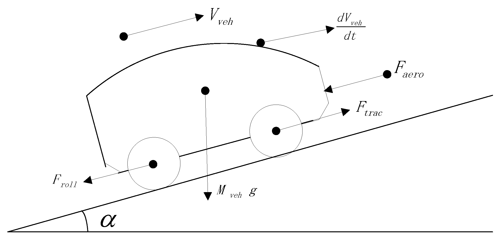
The energy consumption of a vehicle can be estimated from its longitudinal dynamics, illustrated in Figure 1. By the Newton’s law, we have the equation
where is the vehicle mass, the vehicle speed, the rolling friction, the aerodynamic drag, the force caused by the road slope, and the traction force generated by the powertrain.
The rolling friction force is calculated as
where g is the gravity acceleration, the road grade angle in radiant, and the rolling friction coefficient, which is assumed constant in this paper. The aerodynamic drag is directly proportional to the square of the vehicle’s relative speed with the air, namely
where is the density of the ambient air, the air resistance coefficient, and the frontal area of the vehicle. The force induced by the gravity on a slope is the following. The road grade angle is positive (negative), when the vehicle goes uphill (downhill).
Let be the vector of all relevant vehicle parameters. If is given and the vehicle has no regenerative brake, the energy consumption of the vehicle finishing the trip along the varying road angle trajectory is
where is calculated by Equation (8).
The objective is to minimize the total energy consumption of all vehicles traveling on the road during the life time of the road, which is a stochastic process. We consider as a random vector with the probability distribution function
Therefore, is also a random variable. The objective function is the mean value of all vehicle energy consumptions under the probability distribution , namely
where E represents the expectation of a random variable.
In practice, the 4D probability distribution function is difficult to obtain and the corresponding expectation complicated to compute. We simplify it to a 1D probability distribution function as follows. Suppose that all vehicle parameters are bounded within ranges, i.e., , , , and . Assume that all parameters are linearly proportional to vehicle weight. Since the tire rolling resistance is inversely proportional to the radius of the tire, we assume that it decreases when weight increases. Define two boundary vectors and . The parameter vector at an arbitrary weight is
Consider as the only random variable with the probability distribution function
Then the mean value of all vehicle energy consumptions on the road is reduced to
2.3. The Optimal Control Problem
The optimal trajectory of road grade angles to minimize the total energy consumption of all vehicles running on it can be solved as an optimal control problem. The control input is the continuous function of road grade angle , . The road grade angle is limited in the range , where and . The state space equation is given in Equation (7) and the process is a second-order nonlinear process. The constraints on the state vector are , , and . The constraint on the final value of requires identical altitude of the origin and the terminal. This is necessary for round trips. The constraint is also applicable if the road is bidirectional.
3. Analytical Solution
This section simplifies the optimal control problem in Equation (15) and finds the analytical solution of the simplified problem by Pontryagin’s minimum principle (PMP) [31]. The analytical solution provides insight into the problem and verifies the numerical solutions presented in Section 4. Analytical solution may be found only if the state space model, the objective function, and the velocity profile are very simple. See [32,33,34] for examples of finding analytical solutions to minimize vehicular energy consumption.
We apply the following simplifications to the problem in Equation (15).
- Only one vehicle is considered in Equation (15a). The expectation computation in the equation is then unnecessary.
- The absolute value of the road grade angle in radiant is very small, i.e., and . Consequently, and for all .
Owing to the second simplification, the differential equation of the vehicle speed in Equation (15b) is reduced to
whose solution is function calculated by Equation (3). The computing method of ensures for all . The optimal control problem in Equation (15) is then simplified to
s.t. for all ,
This section finds the analytical solution to the simplified control problem by PMP. For convenient presentation, we rewrite the expression of as
where
To remove the nonlinear function max in Equation (16a), we introduce the following assumptions on the sequence of accelerations.
Assumption .
For all , if , then it must satisfy the inequality
Assumption .
For all , if , then it must satisfy the inequality
Let be the maximal vehicle speed during the road.
Assumption .
For all , if , then it must satisfy the inequality
These assumptions are easily satisfiable for common driving scenarios. For instance, consider a small car with the following parameters: , , m, m/s, kg, kg/m, and km/h. Then Assumption 1 implies that if the vehicle is accelerated, the acceleration must be no less than m/s. This is a very small value for vehicle acceleration. Assumption 2 implies that if the vehicle is braked, the acceleration must be no more than m/s. The constraint is easily satisfiable by the vehicle’s brake. In Assumption 3, when the minimal road is , the traction force is N and obviously less than 0.
Assumption 1 ensures that the traction force is not negative during acceleration, and Assumption 2 ensures that the traction force is not positive during deceleration. Assumption 3 requires that the absolute value of the angle of the steepest downhill is so large that brake must be applied to keep constant speed. The statements are formalized as the following propositions.
Proposition 1.
For all , if and Assumption 1 holds, then it must be true for all .
Proof.
By the definition of in Equation (17), we have
If , then . If and Assumption 1 holds, we apply the inequality of Assumption 1 to the previous equation.
Because , we have . Because , we have . Moreover, because and , we also have . Consequently, we obtain the final statement , . ☐
Proposition 2.
For all , if and Assumption 2 holds, then it must be true for all .
Proof.
The proof is very similar to the proof of Proposition 1. If , then . If and Assumption 2 holds, we have the inequality
Since , , and , we obtain the final statement , . ☐
Proposition 3.
For all , if and Assumption 3 holds, there must exist a unique angle such that , for all , and for all .
Proof.
Since , for all . Because , Assumption 3 yields
Evidently . The derivative of the traction force to angle is
Because , and , we can show
Consequently, is a monotonically increasing and differentiable function. There must exist a unique zero point such that
Since both and are positive, it must be true . The value of can be obtained by solving the nonlinear equation; however, when , the nonlinear equation is approximated as a linear equation
and its solution is
Finally, the monotonicity of ensures and . ☐
The Hamiltonian of the control problem in Equation (16) is
where is the costate function. Note that the Hamiltonian is independent of . By PMP, the optimal costate function satisfies the differential equation
Consequently, the optimal costate function is a constant over the entire road and its value will be determined by solving a nonlinear equation at the end of this section. The optimal road grade angle at any position is
This minimization problem is solved in three cases depending on the value of acceleration .
3.1. Positive Acceleration
If , then Assumption 1 and Proposition 1 ensure that is non-negative and the minimization problem in Equation (20) becomes
where , , , and are defined in Equation (17). The term disappears at the second equation, because it is independent of . A necessary condition of the minimum point is where the first derivative of H being zero.
Since both and are positive in this case, we have . Three possible cases arise depending on the value of .
- (1)
- If , thenEquation (21) has no solution in the range and the Hamiltonian is monotonically increasing in the range. The minimum point is hence .
- (2)
- If , thenEquation (21) has no solution in the range and the Hamiltonian is monotonically decreasing in the range. The minimum point is hence .
- (3)
- If , then the solution to Equation (21) is
Furthermore, the second derivative of H at is
Consequently, must be a local minimum point. We can further prove that at this case is the global minimum point in the range .
Proposition 4.
If is positive and exists, then .
Proof.
Since , for any , we have the inequality
and hence
Similarly, for any ,
and hence
The two inequalities imply that is the global minimum point of H, i.e., . ☐
Summarizing the three cases, we have the minimum point of as
3.2. Negative Acceleration
If , then Assumption 2 and Proposition 2 ensure that is non-positive and the minimization problem in Equation (20) becomes
Its solution depends on the value of .
The symbol * in the last case represents an arbitrary value in .
3.3. Zero Acceleration
If , Assumption 3 and Proposition 3 ensure that there is a unique angle such that and and . The Hamiltonian is then a continuous function of two cases.
Note that .
Let be the minimum point of and the minimum point of . The global minimum of the Hamiltonian is
and the global minimum point is
The values of and are dependent on . Three cases follow.
- (1)
- If , is then monotonically increasing in and . The derivative of to isBecause , , and , we haveConsequently, . Since H is a continuous function,In this case, we have
- (2)
- If , and . By the definition of , we have for all . Consequently,where * represents an arbitrary value.
- (3)
- If , is then monotonically decreasing in and . The minimum point of in is identical to Equation (23), except that and is replaced by .
3.4. The Value of
Section 3.1, Section 3.2 and Section 3.3 show that the minimum road angle of the Hamiltonian in Equation (20) is dependent on the value of . The following properties related to the value of can be proved.
Lemma 1.
If and there are at least two accelerations and , , such that and , then the solution to Equation (20) is not unique.
Proof.
Since and , Equation (24) states that is arbitrary in at .
Since , the vehicle speed at any position is a the constant . Since ,
The zero point must exist and Equation (25) states that is arbitrary in at .
Since the optimal angles at two sections can be arbitrary, the total solution of () is not unique. ☐
Lemma 2.
Proof.
We show this lemma in three cases depending on the value of acceleration at position .
- (1)
- : The minimum point to Equation (20) is given by Equation (23). In the first case of the equation, if , then the value of belongs to this case. Consequently, must be . If , then the value of may belong to the first or the third case. It cannot belong to the second case, because it is always true . Therefore, or . By Equation (22), if , then .
- (2)
- (3)
- : The minimum point to Equation (20) is found in Section 3.3. If ,
In summary, the optimum road angle is always negative for the entire road. ☐
Lemma 3.
If and there is at least one accelerations , , such that , then the solution to Equation (20) has the property for all and for all .
Proof.
We show this lemma in three cases depending on the value of acceleration at position .
- (1)
- (2)
- (3)
Since the negative acceleration exists, we must have for . In summary, the optimal road angle is always non-negative during the road and positive during the deceleration segment. ☐
Theorem 1.
If there are at least two accelerations and , , such that and , the optimal control problem in Equation (16) with the altitude constraint in Equation (16d) has a unique solution only if .
Proof.
If , the solution is not unique by Lemma 1. If , the optimal road angle function has the property according to Lemma 2. Applying integration to Equation (16b), we have the identity
Therefore, and it violates the constraint in Equation (16d).
If , Lemma 3 ensures that and . This yields the inequality and it violates the constraint in Equation (16d).
In summary, the necessary condition for the existence of a unique optimal road angle function to Equation (16) is . ☐
With the new knowledge of Theorem 1, we summarize the optimal road angle function in one equation depending on acceleration . At any ,
In the equation, if is very large, the argument in the arcsin function may be larger than 1. Then takes the second value in the max function.
Equations (16b) and (16d) yield a nonlinear equation of .
The tricky part of establishing this equation is that at the segments where are dependent on , which is yet unknown. Conjecture on the value of and iterations are necessary to find . We start with conjectures on for the segments where and construct the equation as in Equation (28). After solving the equation, we verify if the conjectures are correct. If so, we have found a candidate of the optimal costate . Moreover, since PMP and Theorem 1 provide only necessary conditions on the optimal costate, there may be multiple candidates satisfying Equation (28) and all relevant constraints derived from Equation (27). In this case, we must compute the energy consumptions by Equation (16a) for all these candidates and identify the one with the minimal energy consumption.
There are more complicated cases where the optimal angle value switches from one extreme to the other. For example, if in the segment , then we know is monotonically increasing in the segment . If there exists a position such that for and for , then a corresponding equation can be constructed and solved. Among the n acceleration values of the sequence , , if there are accelerations that are positive, we repeat the equation solving process at least times.
3.5. An Illustrative Example
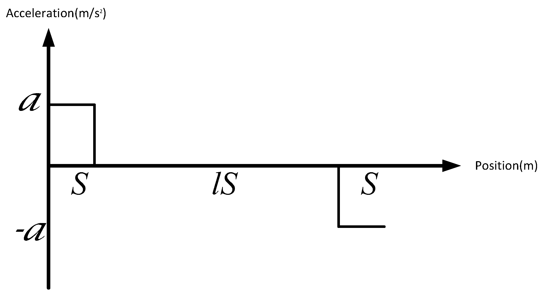
Figure 2 shows the acceleration sequence corresponding to the position sequence , where , , and . Evidently, the road is divided into segments for this example. Let . The speed sequence by Equation (2) is .
Let . By Equation (3), when . By Equation (27), the optimal angles in segment are negative and the optimal angle in segment is . Therefore the optimal angle during the first segment cannot be always . We further assume that the optimal road angle in the first segment is always larger than , i.e.,
Since , we have the approximation
and
The vehicle speed is constant in segment . The optimal road angle in the segment cannot be determined yet.
Since , we have the approximation
and
The optimal road angle in the last segment is constant . The change of the road altitude during this segment is
The solutions to Equations (29a) and (29b) are
and
respectively. The two solutions must both satisfy the inequalities
where . Since the second inequality must hold for all and , it is reduced to
The two solutions also individually satisfy the following two inequalities.
To complete the example, we use the vehicle parameters given behind Assumption 3. Let m/s and the maximal speed be km/h m/s. Then m. Solving the problem with different values of l, we find the following results.
- When , is the only valid costate value and hence the optimal one. The optimal road angle function is
- When , is the only valid costate value and hence the optimal one. The optimal road angle function is
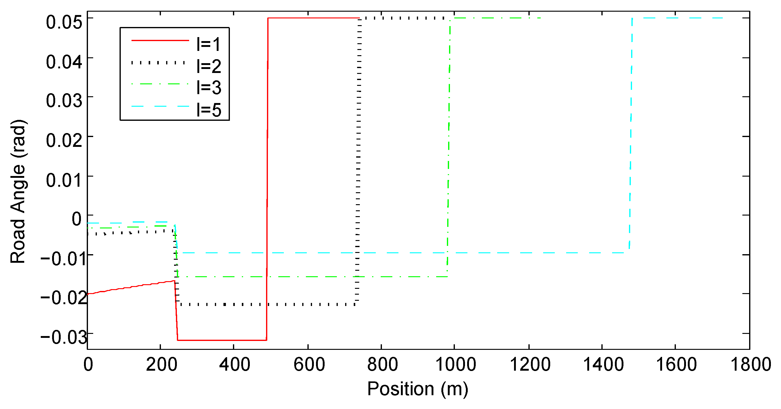
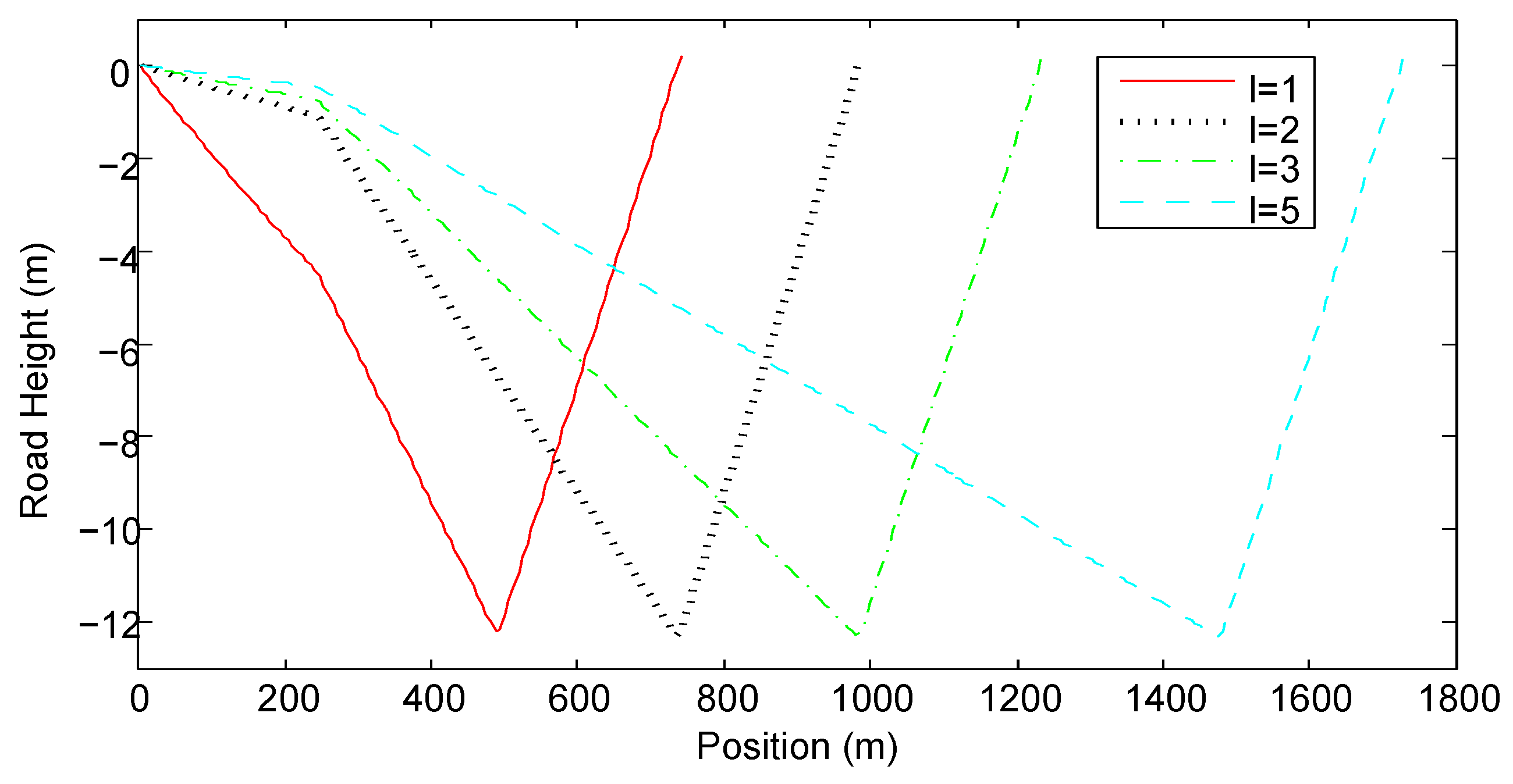
Figure 3 and Figure 4 show the optimal road grade and the optimal road height with different values of l, respectively. When , the road angle is about rad during the acceleration segment. During the constant speed segment, the road angle is about rad and during the deceleration segment, the road grade reaches its maximal limit. When , the road angle is approximately within the range in the acceleration and constant-speed segments. During the deceleration segment, the road angle always reaches the its maximal limit. The larger is the value of l, the larger is the road angle in the acceleration and constant-speed segments. Contrary to intuition, the optimal road has steeper downhill during the constant speed segment than during the acceleration segment. Figure 4 shows that regardless of the length of the road, the lowest road height is identical, because it is determined by the length of S and the maximal road angle .
Recall that the optimization problem in Equation (16) ignores the speed dynamics in Equation (15b). Figure 5 justifies the validity of the simplification. In the figure, the numbers correspond to different values of l , reference speed means the velocity of the vehicle running on the flat road and actual speed means the velocity of the vehicle running on the optimal road. For example, the annotation "Reference speed 1" represents the velocity of the vehicle running on the flat road when . Figure 5 shows the relationship between actual speed and reference speed. Evidently, the actual speed is very close to the reference speed. Table 1 provides RMSE and normalized RMSE between the reference and actual speeds.
Finally, we validate the correctness of the optimal road angle function by comparing energy consumption with two reference road profiles. The first one is the flat road. The second one is the road that has the minimal/maximal angle during the acceleration/deceleration segments and zero angle during the constant-speed segment. We call it the symmetric road. Its corresponding road angle is provided in Equation (32). The results are listed in Table 2. Evidently the road profile obtained by PMP results in the least energy consumption.
4. Numerical Analysis
In the previous section, the analytical solution is obtained for only one vehicle driving at a given acceleration profile. Recall that our ultimate objective as formulated in Equation (15) is to find the optimal road angle profile to minimize the total energy consumption of all vehicles running on the road. This problem is too complex to solve by the same analytical solution. This section solves the road angle optimization problem with deterministic dynamic programming (DP). The section contains four parts. Section 4.1 presents the discrete-time model of the optimal road grade design problem suitable for DP. Section 4.2 solves the illustrative example in Section 3.5 again by DP. The comparison of the analytical and DP solutions confirms the correctness of the DP solution. Section 4.3 presents a general problem with a larger number of different vehicles and solves the problem by DP. Section 4.4 applies the Monte Carlo method to verify the correctness of the DP result by a large number of simulations. The simulation results prove that the total energy consumption of all vehicles running on the optimal road is smaller than energy consumption on the flat road and the reduction is achievable even though the assumed vehicle speed profile and weight distribution are not satisfied. When we compare energy consumption of all vehicles driving on the optimal road and those on the symmetric road, the simulation results show that the optimal road results in less energy consumption in most cases. Small exceptions may appear if the driving condition is significantly different from the assumption.
4.1. Model for DP
Dynamic programming (DP) is a powerful optimal control method that can handle complex models and constraints [35]. This section elaborates our approach to solve the optimal control problem in Equation (15) by DP. We first transform both the continuous-time optimal control problem and the continuous-time state-space equation into a discrete-time optimal control problem. The time variable is in fact the distance. The number of discretization steps is calculated by , where is the traveling distance and is a small positive distance that can divide . The continuous road angle function is discretized into a sequence of , . The road grade angle is limited in the range , where and . The continuous state-space equation in Equation (15b) is discretized into
where is the square of the speed at the distance , , and .
The objective function in Equation (15a) should be converted from the continuous function into a discrete function. First, the weight distribution function in Section 2.2 is discretized by W points of distinct weights, which satisfy the relation: . The probability of is for , and .
4.2. Numerical Solution to the Illustrative Example
We use a generic dynamic programming MATLAB (DPM) function [36] to solve the optimal control problem in Equation (33) for the illustrative example in Section 3.5. Only one set of vehicle parameters is used in Equation (33), i.e., the probability of vehicle weight being 750 kg is 1. Other vehicle parameters are identical to those in Section 3.5. According to the result in Section 3.5, the height is within the range [−13, 0] m and divided by 131 points. Each step in height is 0.1 m. According to Figure 5 and Table 1, the difference between the actual and reference vehicle speeds is very small. We then set the discretization grid of as a dynamic range , where is obtained by Equation (3) for and is a small positive number estimated from Table 1. The range is discretized by 101 points at one step. The control signal is divided by 501 points. Thus, a step of is rad.
The numerical solution for Equation (33) by DP is very close to the analytical solution presented in Section 3.5 and the comparison is shown in Figure 6. The small difference is due to the numerical error of DP. When the vehicle has positive acceleration or constant speed, the corresponding road angle is negative. In the deceleration region, the optimal road grade reaches the highest positive grade. Table 3 shows the comparison of DP and the analytical solution. Table 4 presents the results of the traveling time with three distances. The influence of the optimal road angle profile to traveling time is very small and the longer is the distance, the smaller is the influence on traveling time.
4.3. Numerical Solution to the General Problem
Section 4.2 considers only one vehicle. This section uses DP to find the optimal road angle profile between two points for a larger number of different vehicles. The acceleration profile is identical to that in Figure 2 and the maximal vehicle speed is 80 km/h. The parameter l is 5, corresponding to the direct distance of around 1700 m between the origin and the terminal. The distance is common between two bus stops. Suppose that the vehicle weights are between 750 kg and 40 t. The range is discretized by 10 distinct points, whose probabilities are listed in Table 5. The corresponding vehicle parameters are also given in the table. The probability values of the vehicle weights are estimated by our observation of common urban traffic. The vehicle frontal area and aerodynamics coefficient are increasing with the vehicle weight, but the tire rolling resistance is decreasing with the vehicle weight.
In this problem, the height is within the range m and divided by 131 points. Each step in height is 0.1 m. We then set the discretization grid of as a dynamic range . The range is discretized by 101 points for one step. The control signal is divided by 501 points. Thus, a step of is rad. Applying these values in DPM, we obtain the optimal trajectories of road angle and height plotted in Figure 7 as blue solid lines. The trajectories of road angle and height of the symmetric road are also plotted in Figure 7 as the red dashed lines. The optimal results agree well with the DP solution in Figure 6 when and the difference is because the result in Figure 7 considers the mean value of various vehicle weights.
4.4. Monte Carlo Simulation
We verify the correctness and advantage of the DP solution in Section 4.3 via Monte Carlo simulations on a large number of vehicles with various weights. The simulations cover three scenarios. Section 4.4.1 simulates a large number of vehicles with random weights whose probability distribution function is consistent with Table 5. Section 4.4.2 simulates the scenario where the distribution of vehicle weights is inconsistent with Table 5. Section 4.4.3 simulates the scenario where all vehicles must make an extra stop during the travel.
4.4.1. Weight Probability Distribution Similar to the Assumption
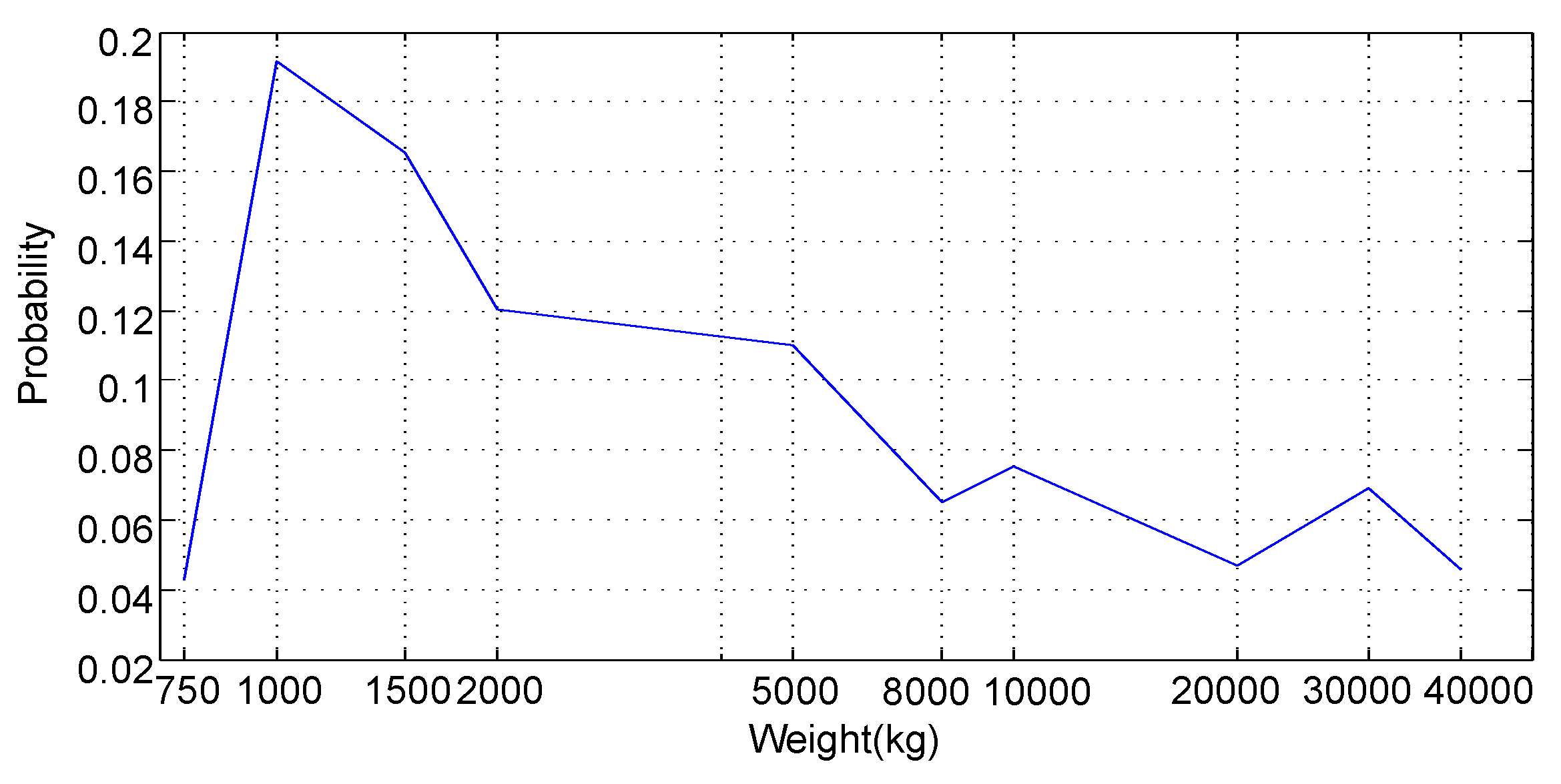
In the first scenario, we simulate a large number of vehicles whose weights satisfy a probability distribution function that is consistent with Table 5. Figure 8 illustrates the occurrence ratio of the weights of 1000 randomly generated vehicles. To clearly show weights from 750 kg to 40 tonnes, the weight axis is in logarithmic scale. To demonstrate the advantage of the optimal road angle profile, we compare the energy consumptions of the same set of randomly generated vehicles on the optimal road, the symmetric road, and the flat road, respectively. The numbers of random vehicles range from 1000 to , as listed in Table 6. For each number, e.g., 1000, we generate 10 sets of random vehicles and each set contains the given number, e.g., 1000, of vehicles. For each set of vehicles, we calculate the average energy consumptions of all vehicles for three types of roads. The mean values and standard deviations of the 10 random vehicle sets for the three types of roads are listed in Table 6. The energy reduction percentages of the optimal road compared with the flat road as well as that compared with the symmetric road are indicated by the corresponding values in the last column in Table 6. The value at the row of “Flat Road”/“Symmetric Road” is the reduction percentage of the optimal road compared to the flat/symmetric road.
It is evident from Table 6 that vehicles running on the optimal road can save about and energy compared with vehicles running on the flat road and the symmetric road, respectively. Note that the standard deviation in the table decreases when the number of simulated vehicles increases. This implies that the simulation result with a larger number of vehicles is more accurate.
4.4.2. Weight Probability Distribution Different from the Assumption
In order to verify that the optimal road profile is robust, we simulate a large number of vehicles whose weights satisfy a probability distribution function that is inconsistent with Table 5 in this section. We consider four cases: normal distribution, exponential distribution, uniform distribution, and lots of trucks and less light vehicles.
In the case of normal distribution, the mean and standard deviation are 1500 and 500 kg, respectively. Figure 9 illustrates the weights of 1000 randomly created vehicles satisfying the normal distribution. The minimal weight is 750 kg.
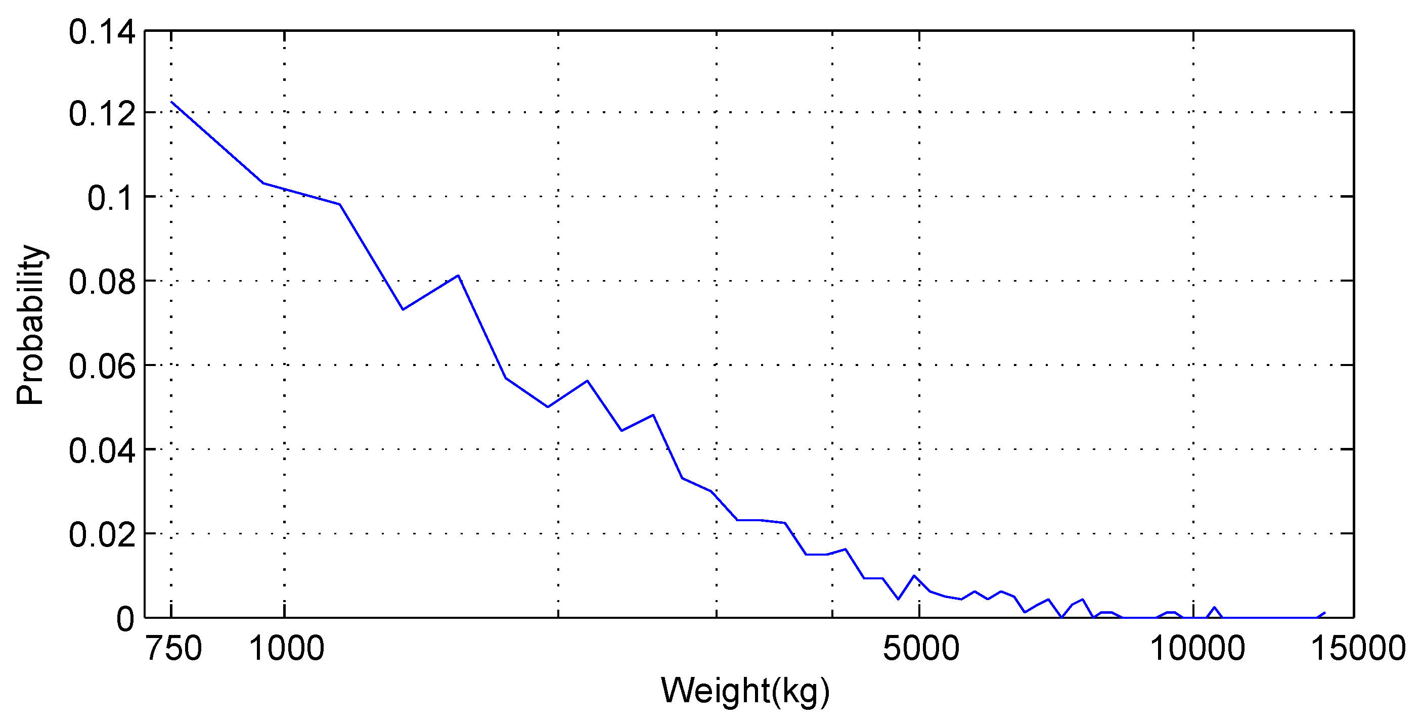
In the case of exponential distribution, the probability distribution function is . The definition ensures that the weight is at least 750 kg. The value of is . Therefore the mean weight of the distribution function is kg. Figure 10 illustrates the weights of 1000 randomly created vehicles which satisfy the exponential distribution.
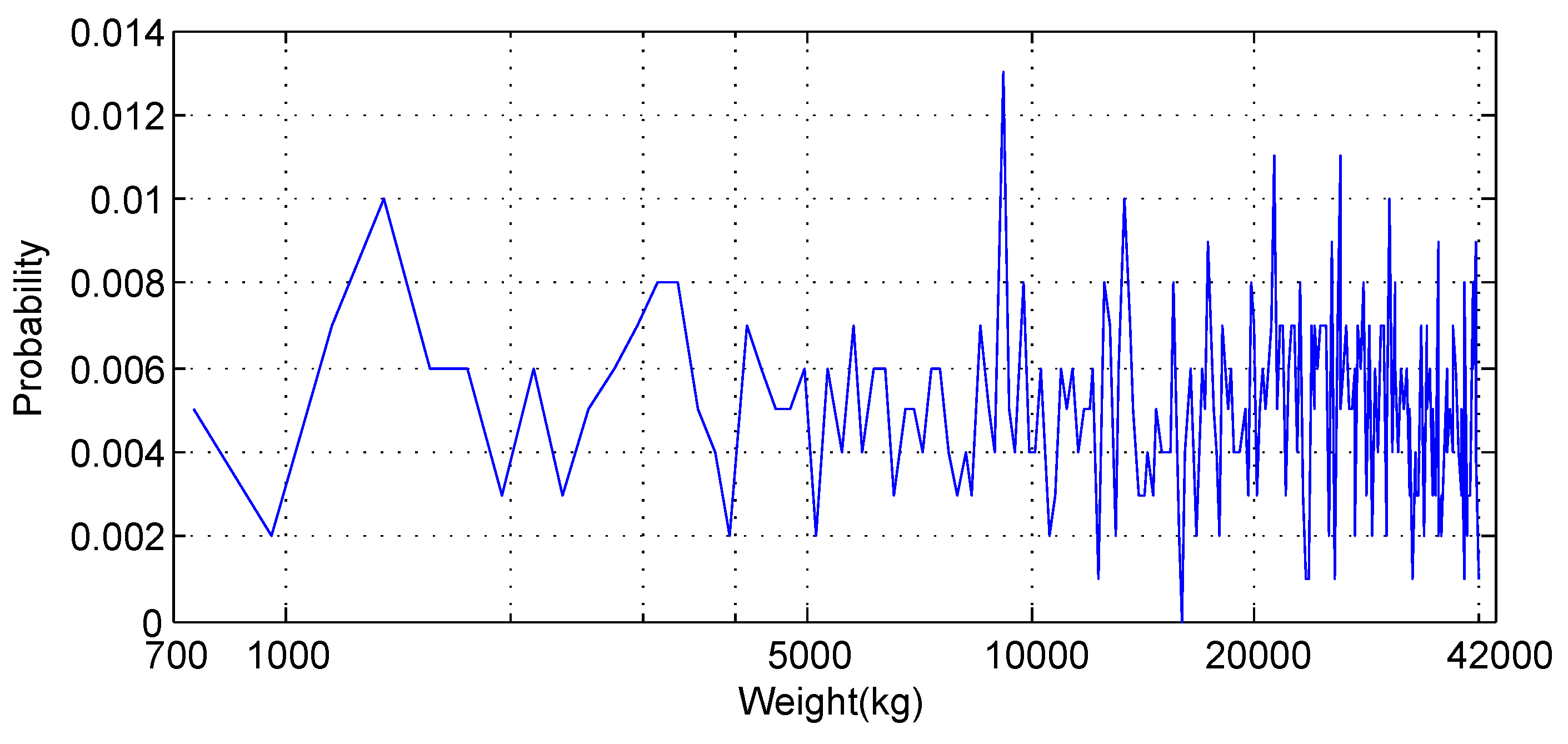
In the case of uniform distribution, the vehicles are uniformly distributed between 750 kg and 40 tonnes. Figure 11 illustrates the weights of 1000 randomly created vehicles which satisfy the uniform distribution. Finally, we simulate the scenario that there are much more heavy trucks on the road than light-weight passenger cars. The weight distribution function of 1000 random vehicles is plotted in Figure 12.
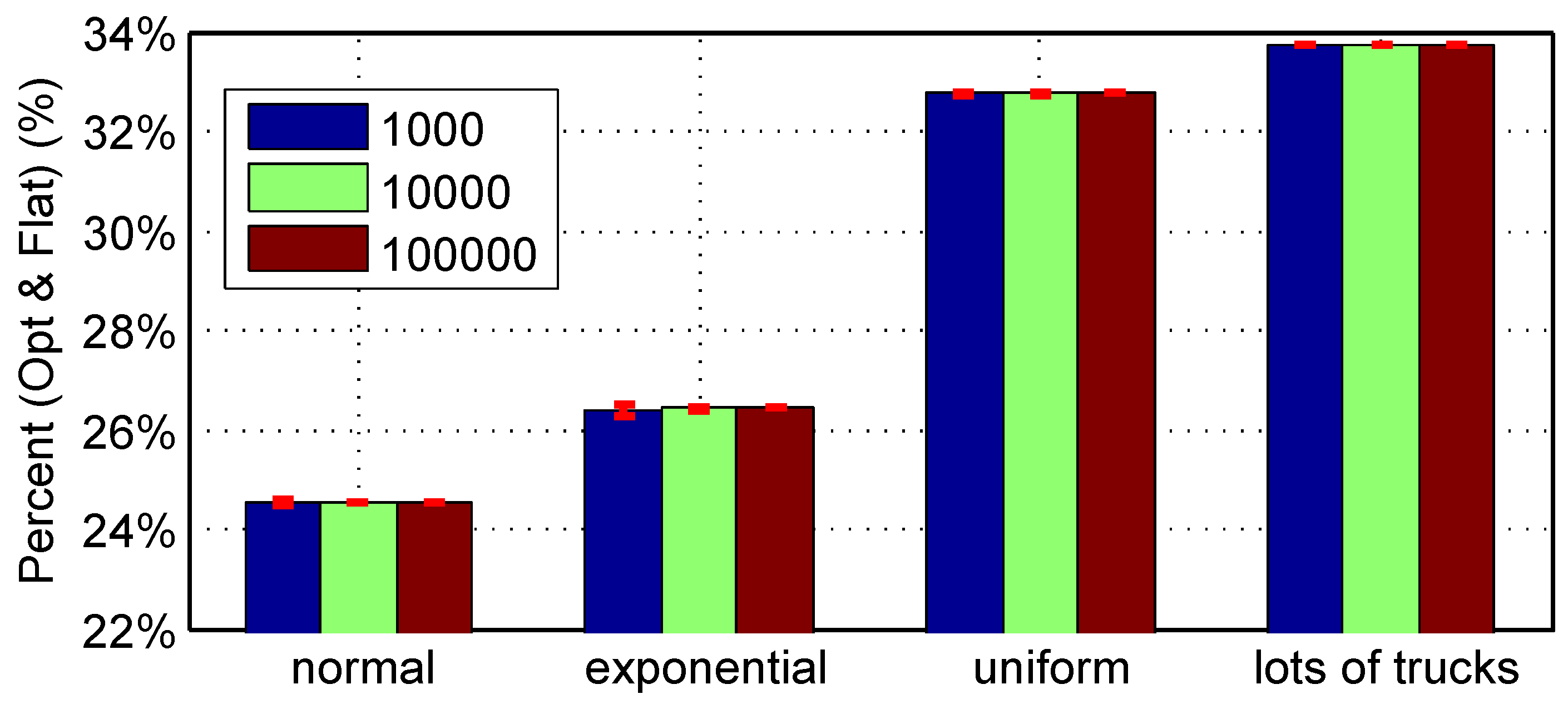
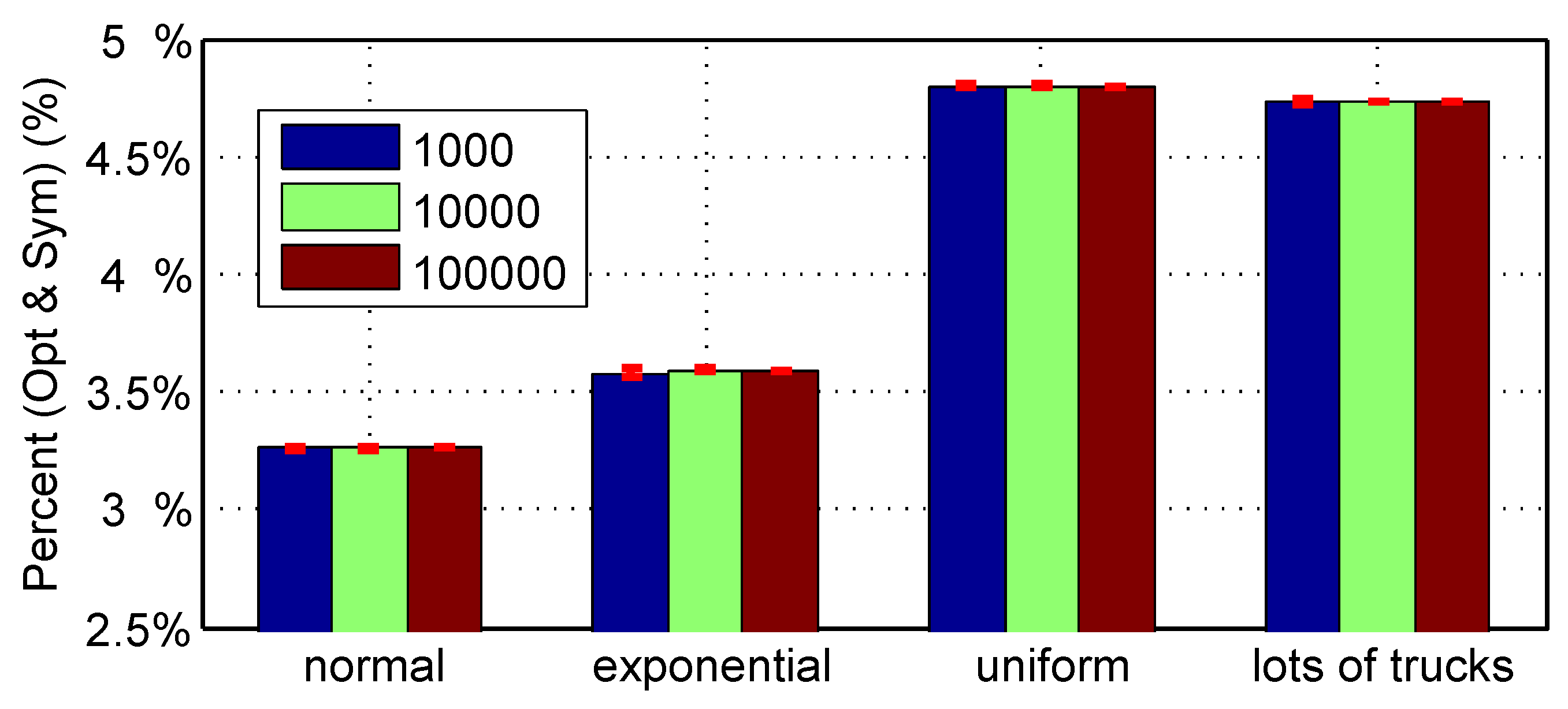
We repeat the same simulations and calculations described in Section 4.4.1. For each number of simulated vehicles, 10 Monte Carlo simulations are repeated. For every simulation, we calculate the average energy consumptions on the three different roads, namely the optimal road, the symmetric road, and the flat road. From these results, we calculate the reduction percentages of the optimal road compared to the flat and symmetric roads for each simulation. The 10 reduction percentages are then used to calculate the mean and standard deviations of the saving percentages, as illustrated in Figure 13 and Figure 14 and Table 7. The bars and the red line sections in Figure 13 and Figure 14 represent the means and standard deviations of the saving percentages, respectively.
Table 7 shows the standard deviations of energy reductions in Figure 13 and Figure 14. As shown in Figure 13, the energy consumption of all vehicles running on the optimal road is compared to the energy consumption on the flat road. About 24.5% energy is saved in the normal distribution. In the exponential distribution, about 26.5% energy is saved. In the uniform distribution, about 32.7% energy is saved. When there are lots of trucks and less light vehicles, about 33.7% energy is saved. The larger energy reductions for the uniform and lots of trucks cases indicate that the optimal road has larger benefit for heavy vehicles.
Figure 14 shows the mean value of energy reduction of the optimal road compared to the symmetric road. About 3.25% energy is saved in the normal distribution. In the exponential distribution, about 3.6% energy is saved. In the uniform distribution, about 4.8% energy is saved. When there are lots of trucks and less light vehicles, about 4.72% energy is saved.
The Monte Carlo simulations clearly reveal the advantage of the optimal designed road compared to symmetric and flat roads in reducing the total energy consumption of all vehicles running on the road.
4.4.3. Speed Profile Different from the Assumption
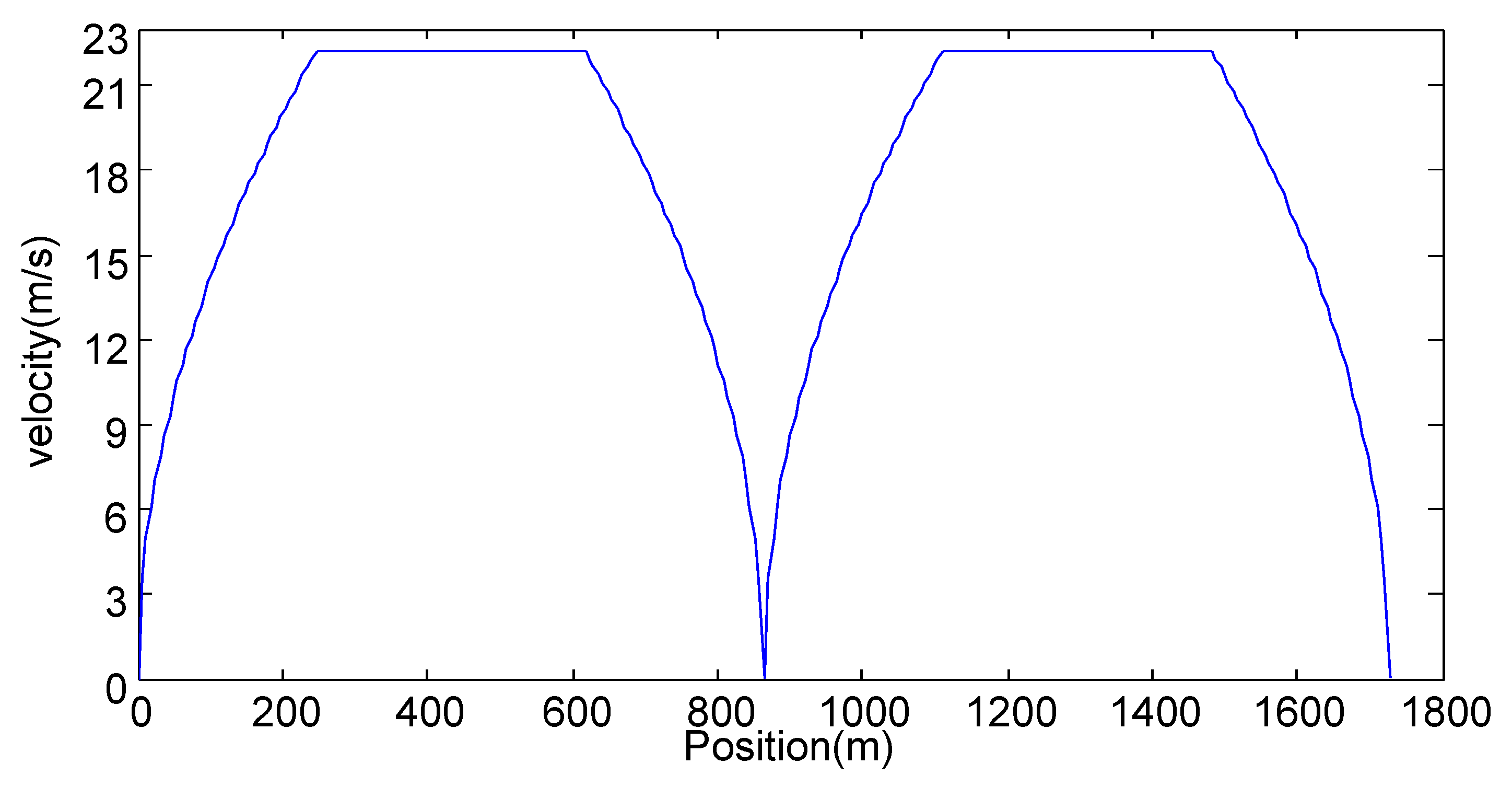
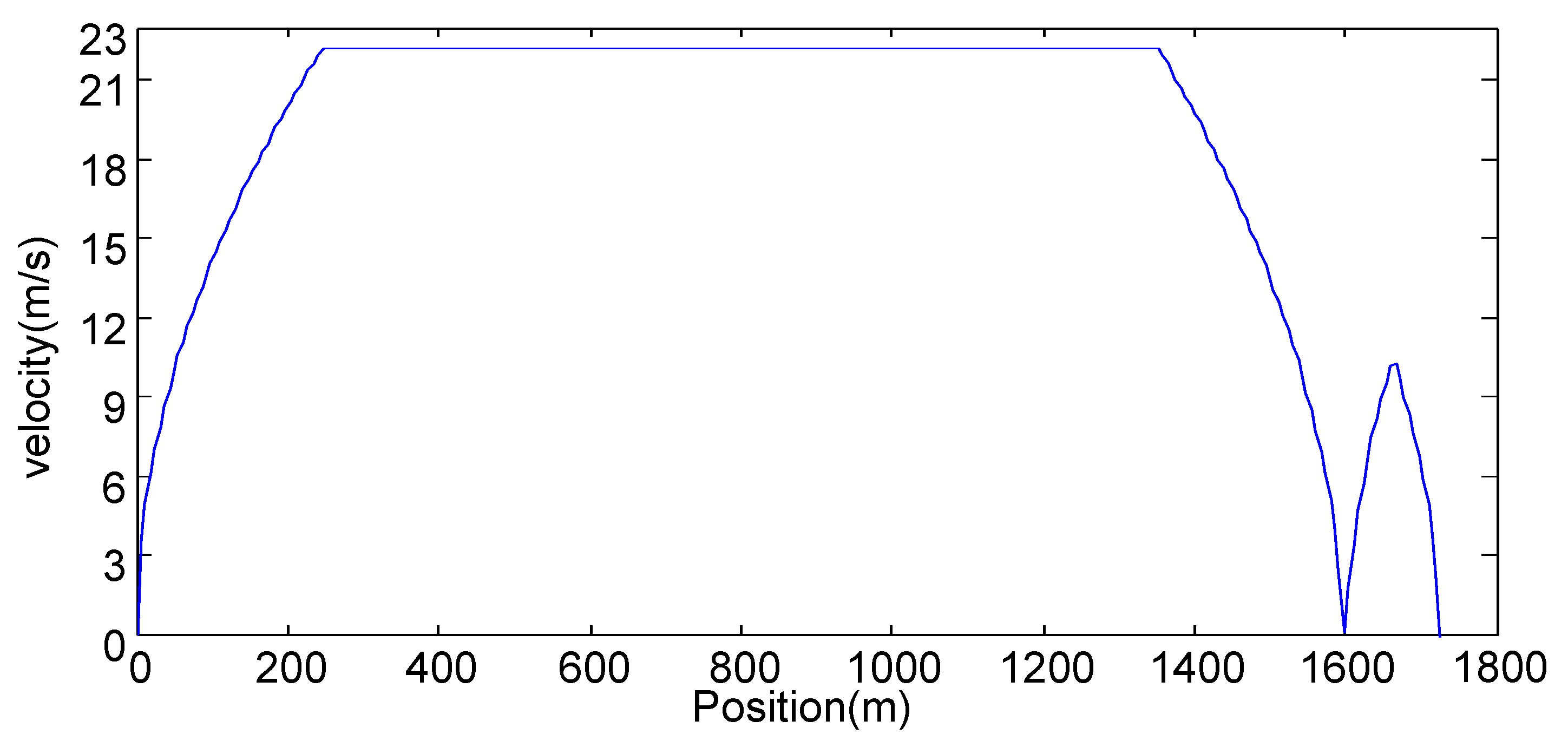
In this part, we simulate the two scenarios where all vehicles must make an extra stop during the travel. The first is an extra stop at the half distance as illustrated in Figure 15. The second is the vehicle stops at the uphill as illustrated in Figure 16. The probability distribution of weights is the same as in Section 4.4.1. We repeat the same Monte Carlo simulations discussed in Section 4.4.1. Table 8 and Table 9 list the simulation results of the means and standard deviations of average energy consumptions on the three types of roads for the two speed profiles, respectively. In Table 8 and Table 9, the energy reduction percentages of the optimal road compared with the flat road as well as that compared with the symmetric road are indicated by the corresponding values in the last column.
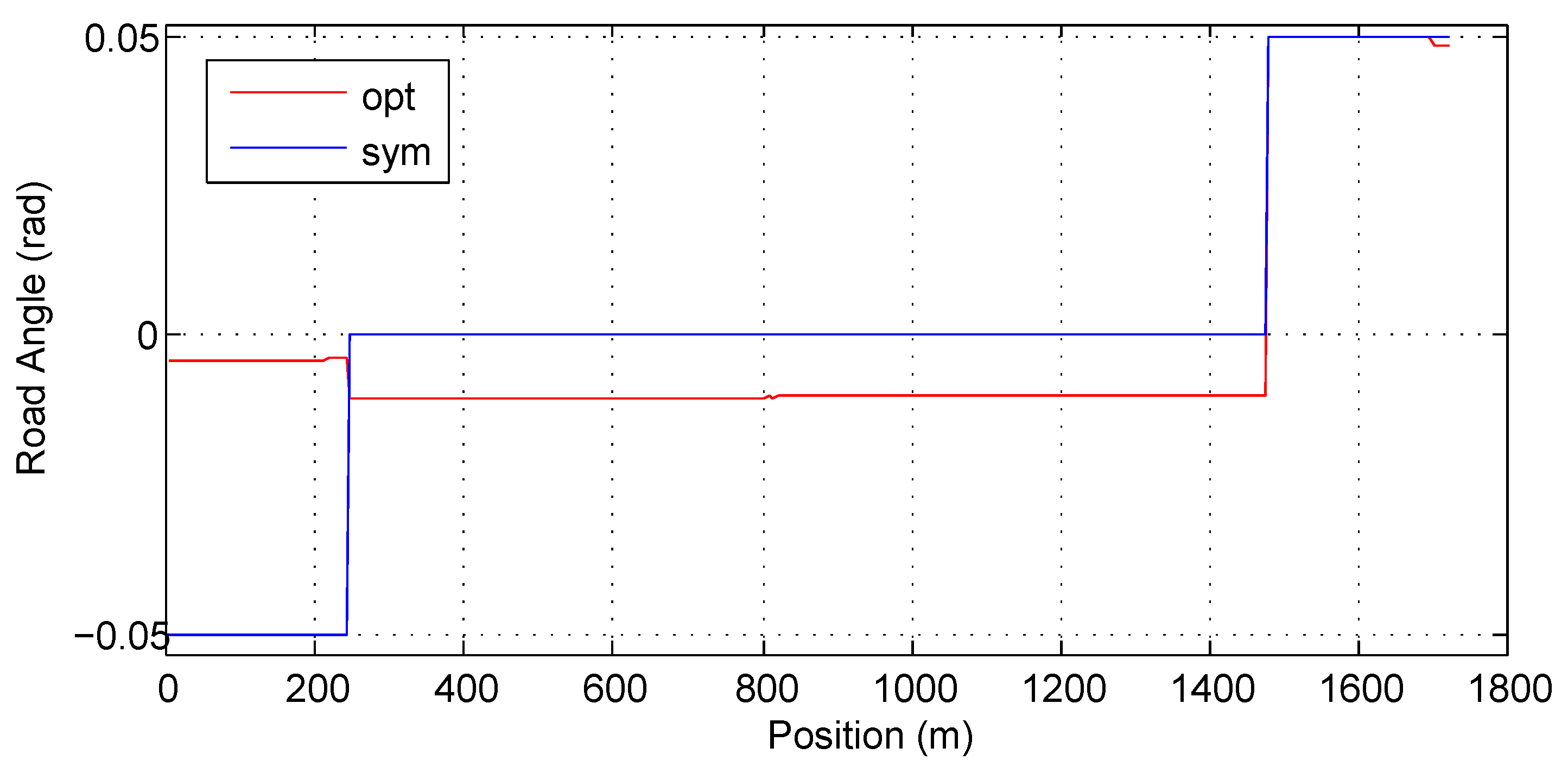
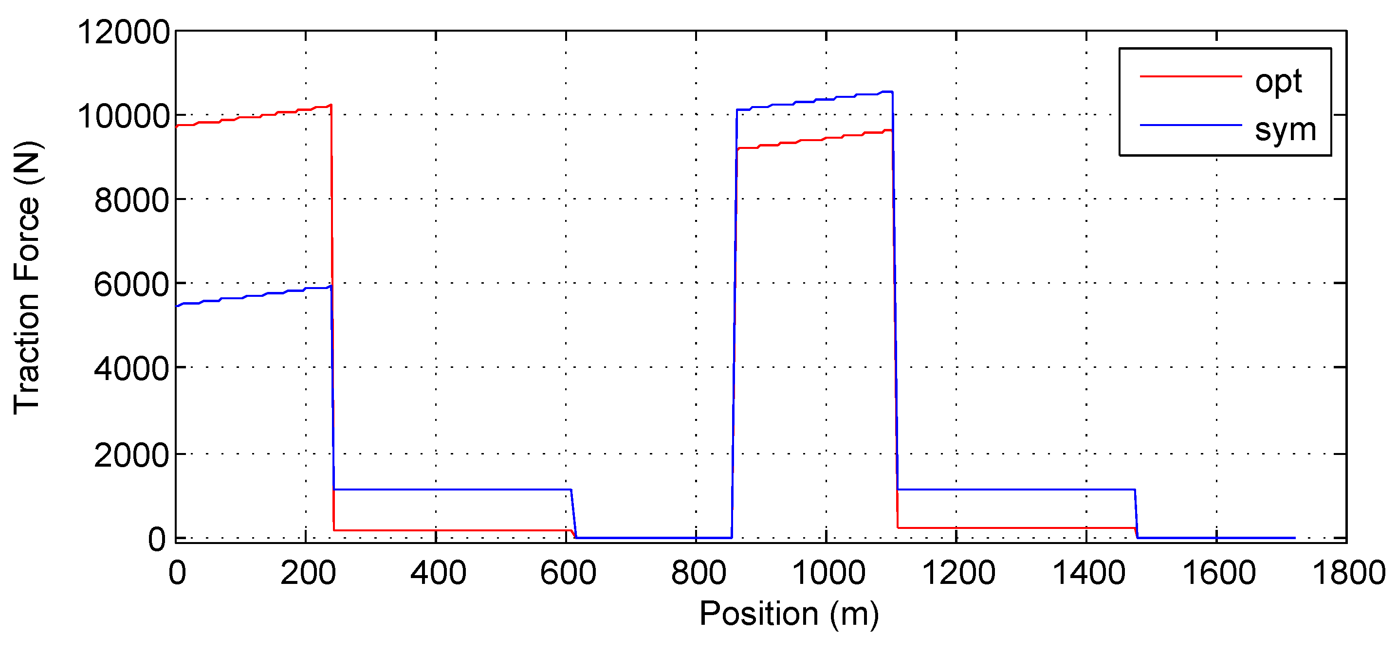
Table 8 shows that the optimal road saves about energy compared with the flat road but consumes about 2.2% more energy compared with the symmetric road. The reason is that the downhill of the symmetric road is steeper than the downhill of the optimal road, as illustrated in Figure 17. The corresponding average traction forces on the two roads are plotted in Figure 18. The energy consumption on the optimal road is larger than that on the symmetric road during the first acceleration. Without the unexpected stop, the energy saving on the optimal road during the constant speed section outweighs the additional consumption at the acceleration section. The unexpected stop, however, reduces the energy saving during the constant speed section and hence results in larger energy consumption on the optimal road than on the symmetric road.
To maintain smaller energy consumption on the optimal road, the distance of the constant speed section needs to be longer. We study the energy consumption comparison between the optimal and symmetric roads for different distances. There is always a stop in the middle of the distance. We simulate 1000 vehicles with the weight distribution as in Section 4.4.1. The results are listed in Table 10. When the distance is 20 km, the energy consumption of the optimal road is again smaller than the symmetric road.
Finally, Table 9 shows that the optimal road saves about 19.2% energy compared with the flat road and about energy compared with the symmetric road when all vehicles make one stop at the uphill during the traveling.
5. Preliminary Cost Analysis
The analysis suggests large reduction of the total energy consumption of all vehicles running on the optimally designed road, but a major concern to road optimization is cost. Road construction is expensive and has many concerns in addition to cost and energy consumption. If we build a new road, the dominating costs are for evacuating assets along the road, hiring the construction company, digging earth and rock, transporting waste and construction materials, paving the road, etc. These costs are independent of the road grade profile and hence our method can be applied with little influence on the cost of building the road. The benefit of the new road design method is obvious in this case. In our future work, we shall include more practical constraints, e.g., the maximal/minimal altitude, the longest distance for downhill/uphill, into the optimization process.
The questionable case is then to rebuild an existing road to obtain the optimal angle profile. We have no expertise in cost estimation of road construction and can only give a very preliminary estimate on it. Take the road in Section 4.3 and Section 4.4 for an example. Its direct distance is around 1.7 km and we estimate its cost by the methods presented in [37]. Relevant data for making the gross estimate are taken from a practical example in China [38]. The example project spends about $10.5 million to build a 8.5 km-long road. Consequently it takes nearly $1.23 million to build 1 km-long road. Thus, the budget of building the 1.7 km-long optimal road is approximately $2.1 million, which is about the same expenses as that for building a flat road, since the grade of the optimal road is very small. For estimating the cost of rebuilding road, the relevant data come from another example of reconstructing a 25.124 km-long road [39]. The additional cost to rebuild the road is very small. In this reconstruction example, it takes about $5.4 million to rebuild the road and hence the average cost is approximately $0.215 million per km. Then the budget to rebuild the 1.7 km-long optimal road is about $0.365 million.
Suppose that averagely 5000 vehicles use the road every day and the road can be in service for 30 years. If the weights of the vehicles satisfy the distribution in Table 5, Table 6 shows about 31.7% reduction of the total energy consumption over 30 years. Assume that the average fuel consumption is 6.5 L gasoline per 100 km. Thus, one vehicle averagely saves 0.0350 L gasoline per day on the 1.7 km optimal road. The total saving for 5000 vehicles per day for 30 years is roughly 1.918 million liter gasoline. The current gasoline price in China is about $0.93 per liter and assume the same price for the next 30 years. The total saving in money is about $1.8 million for 30 years. Since the fuel price will certainly increase in the future, more saving can be achieved. The saving outweighs the cost of rebuilding the road. Moreover, the reduction on energy consumption also reduces harmful vehicle emissions and contributes to cleaner environment.
6. Conclusions and Future Work
This article presents both analytical and numerical solutions to the optimization problem of finding the optimal road grade that minimizes the overall energy consumption of all vehicles running on the road. We assume that all vehicles on the road follow a given acceleration profile between the two given points. In order to find the analytical solution, the optimal control problem is simplified and the Pontryagin’s minimum principle is used to derive the optimal road grade trajectories. Dynamic programming (DP) is utilized to solve the problem numerically. The paper finds that the numerical solution is almost identical to the analytical solution. Then we use DP to find the optimal road angle profile between two points for a larger number of different vehicles. After that we verify the correctness and advantage of the DP solution via Monte Carlo simulations on a large number of vehicles with various weights. Three cases are considered in the Monte Carlo simulations. First, a large number of vehicles with random weights whose probability distribution function is consistent with the assumption. Second, the distribution of vehicle weights is inconsistent with the assumption. Third, all vehicles must make an extra stop during the travel. The simulations reveal that the optimal road saves energy for all cases, except one. Explanation of the exception is given in the paper.
Compared to the flat road, the optimal road reduces the energy consumption of all vehicles by around 31.7%. Thereby the optimal road has advantage in reducing fuel consumption of ground vehicles and has large application potential.
In the future, we will continue to improve fuel economy by the optimal design of the road infrastructural. Firstly, more comprehensive design objectives and constraints coming from road construction techniques will be included in the DP formalism. Secondly, as stated in Section 4.4.3, if the actual speed profile is inconsistent with the assumed speed profile, the energy consumption on the optimal road may not be the least if the traveling distance is short. We will thus investigate robust road optimization method for reducing the total energy consumption of vehicles with more complex and stochastic velocity trajectories. Thirdly, the optimal road grade profile is dependent on the driving direction. If we design an optimal road between two destinations for both driving directions, the road profiles for both ways are distinct. The implication of the asymmetric design will be further analyzed.
Acknowledgments
This work is supported in part by the National Natural Science Foundation of China under Grant 61374068, Grant 61472295, and Grant 61673309, in part by the Recruitment Program of Global Experts, and in part by the Science and Technology Development Fund, MSAR, under Grant 078/2015/A3. Lei Feng is partly supported by the XPRES project.
Author Contributions
The idea of optimizing the road grade profile to minimize the total energy consumption of all vehicles was initiated by Lei Feng. Junhui Liu developed the numerical solution by dynamic programming and verified the correctness by Monte Carlo simulations under the guidance of Lei Feng and Zhiwu Li. Junhui Liu and Lei Feng jointly developed the analytical solution by PMP. Junhui Liu wrote the draft of the article, which was substantially and repeatedly edited by Lei Feng and Zhiwu Li.
Conflicts of Interest
The authors declare no conflict of interest.
References
- Sciarretta, A.; Guzzella, L. Control of hybrid electric vehicles. IEEE Control Syst. 2007, 27, 60–70. [Google Scholar] [CrossRef]
- Pisu, P.; Rizzoni, G. A comparative study of supervisory control strategies for hybrid electric vehicles. IEEE Trans. Control Syst. Technol. 2007, 15, 506–518. [Google Scholar] [CrossRef]
- Wang, R.; Lukic, S.M. Dynamic programming technique in hybrid electric vehicle optimization. In Proceedings of the 2012 IEEE Conference on Electric Vehicle, Greenville, SC, USA, 4–8 March 2012; pp. 1–8. [Google Scholar]
- Van Keulen, T.; De Jager, B.; Foster, D.; Steinbuch, M. Velocity trajectory optimization in hybrid electric trucks. In Proceedings of the 2010 American Control Conference, Baltimore, MD, USA, 30 June–2 July 2010; pp. 5074–5079. [Google Scholar]
- Liu, J.; Peng, H. Modeling and control of a power-split hybrid vehicle. IEEE Trans. Control Syst. Technol. 2008, 16, 1242–1251. [Google Scholar]
- Gessat, J. Electrically Powered Hydraulic Steering Systems for Light Commercial Vehicles; SAE Technical Paper 2007-01-4197; SAE: Warrendale, PA, USA, 2007. [Google Scholar]
- Petit, N.; Sciarretta, A. Optimal drive of electric vehicles using an inversion-based trajectory generation approach. IFAC Proc. Vol. 2011, 18, 14519–14526. [Google Scholar] [CrossRef]
- Sciarretta, A.; Guzzella, L.; Baalen, J.V. Fuel optimal trajectories of a fuel cell vehicle. In Proceedings of the AVCS, Buenos Aires, Argentina, 28–31 October 2004. [Google Scholar]
- Trichet, D.; Chevalier, S.; Wasselynck, G.; Olivier, J.C.; Auvity, B.; Josset, C.; Machmoum, M. Global energy optimization of a light-duty fuel-cell vehicle. In Proceedings of the 2011 IEEE Vehicle Power and Propulsion Conference (VPPC), Chicago, IL, USA, 6–9 September 2011; pp. 1–6. [Google Scholar]
- Xu, L.; Li, J.; Hua, J.; Ouyang, M. Optimal vehicle control strategy of a fuel cell/battery hybrid city bus. Int. J. Hydrogen Energy 2009, 34, 7323–7333. [Google Scholar] [CrossRef]
- Khodabakhshian, M.; Wikander, J.; Feng, L. Fuel efficiency improvement in HEVs using electromechanical brake system. In Proceedings of the 2013 IEEE Intelligent Vehicles Symposium, Gold Coast, Australia, 23–26 June 2013; Volume 36, pp. 322–327. [Google Scholar]
- Wagner, J.R.; Srinivasan, V.; Dawson, D.M.; Marotta, E.E. Smart Thermostat and Coolant Pump Control for Engine Thermal Management Systems; SAE Technical Papers 2003-01-0272; SAE: Warrendale, PA, USA, 2003. [Google Scholar]
- Nilsson, M.; Johannesson, L. Convex optimization for auxiliary energy management in conventional vehicles. In Proceedings of the 2014 IEEE Conference on Vehicle Power and Propulsion, Coimbra, Portugal, 27–30 October 2014; pp. 1–6. [Google Scholar]
- Khodabakhshian, M.; Feng, L.; Börjesson, S.; Lindgärd, O.; Wikander, J. Reducing auxiliary energy consumption of heavy trucks by onboard prediction and real-time optimization. Appl. Energy 2017, 188, 652–671. [Google Scholar] [CrossRef]
- Bottiglione, F.; Pinto, S.D.; Mantriota, G.; Sorniotti, A. Energy consumption of a battery electric vehicle with infinitely variable transmission. Energies 2014, 7, 8317–8337. [Google Scholar] [CrossRef]
- Koot, M.; Kessels, J.T.B.A.; De Jager, B.; Heemels, W.P.M.H. Energy management strategies for vehicular electric power systems. IEEE Trans. Veh. Technol. 2005, 54, 771–782. [Google Scholar] [CrossRef]
- Hong, T.L.; Nouvelière, L.; Mammar, S. Dynamic programming for fuel consumption optimization on light vehicle. IFAC Proc. Vol. 2010, 43, 372–377. [Google Scholar]
- Hellström, E.; Aslund, J.; Nielsen, L. Design of an efficient algorithm for fuel-optimal look-ahead control. Control Eng. Pract. 2010, 18, 1318–1327. [Google Scholar] [CrossRef]
- Kim, N.; Cha, S.; Peng, H. Optimal control of hybrid electric vehicles based on Pontryagin’s Minimum Principle. IEEE Trans. Control Syst. Technol. 2011, 19, 1279–1287. [Google Scholar]
- Zhang, F.; Liu, H.; Hu, Y.; Xi, J. A supervisory control algorithm of hybrid electric vehicle based on adaptive equivalent consumption minimization strategy with fuzzy PI. Energies 2016, 9, 919. [Google Scholar] [CrossRef]
- Terwen, S.; Back, M.; Krebs, V. Predictive powertrain control for heavy duty trucks. In Proceedings of the IFAC Symposium in Advances in Automotive Control, Salerno, Italy, 19–23 April 2004; pp. 451–457. [Google Scholar]
- Van, K.T.; De, J.B.; Serrarens, A.; Steinbuch, M. Optimal energy management in hybrid electric trucks using route information. Oil Gas Sci. Technol. 2009, 65, 103–113. [Google Scholar]
- Johannesson, L.; Murgovski, N.; Jonasson, E.; Hellgren, J.; Bo, E. Predictive energy management of hybrid long-haul trucks. Control Eng. Pract. 2015, 41, 83–97. [Google Scholar] [CrossRef]
- Sciarretta, A.; Nunzio, G.D.; Ojeda, L.L. Optimal ecodriving control: Energy-efficient driving of road vehicles as an optimal control problem. IEEE Control Syst. 2015, 35, 71–90. [Google Scholar] [CrossRef]
- Dib, W.; Chasse, A.; Moulin, P.; Sciarretta, A.; Corde, G. Optimal energy management for an electric vehicle in eco-driving applications. Control Eng. Pract. 2014, 29, 299–307. [Google Scholar] [CrossRef]
- Gong, Q.; Li, Y.; Peng, Z.R. Optimal power management of plug-in HEV with intelligent transportation system. In Proceedings of the 2007 IEEE International Conference on Advanced Intelligent Mechatronics, Zurich, Switzerland, 4–7 September 2007; pp. 1–6. [Google Scholar]
- Dorle, S.S.; Bajaj, P.; Keskar, A.G.; Chakole, M. Design of base station’s vehicular communication network for intelligent traffic control. In Proceedings of the 9th IEEE Conference on Vehicle Power and Propulsion, Dearborn, Michigan, 7–11 September 2009; pp. 1118–1121. [Google Scholar]
- Horowitz, R.; Varaiya, P. Control design of an automated highway system. Proc. IEEE 2000, 88, 913–925. [Google Scholar] [CrossRef]
- Khan, A.S.; Clark, N. An empirical approach in determining the effect of road grade on fuel consumption from transit buses. SAE Int. J. Commer. Veh. 2010, 3, 164–180. [Google Scholar] [CrossRef]
- Boriboonsomsin, K.; Barth, M. Impacts of road grade on fuel consumption and carbon dioxide emissions evidenced by use of advanced navigation systems. Transp. Res. Rec. J. Transp. Res. Board 2009, 2139, 21–30. [Google Scholar] [CrossRef]
- Saerens, B.; Diehl, M.; Bulck, E.V.D. Optimal control using Pontryagin’s maximum principle and dynamic programming. In Automotive Model Predictive Control; Del Re, L., Allgöwer, F., Glielmo, L., Guardiola, C., Kolmanovsky, I., Eds.; Springer: London, UK; Berlin/Heidelberg, Germany, 2010; pp. 119–137. [Google Scholar]
- Ozatay, E.; Ozguner, U.; Michelini, J.; Filev, D. Analytical solution to the minimum energy consumption based velocity profile optimization problem with variable road grade. IFAC Proc. Vol. 2014, 47, 7541–7546. [Google Scholar] [CrossRef]
- Ozatay, E.; Ozguner, U.; Onori, S.; Rizzoni, G. Analytical solution to the minimum fuel consumption optimization problem with the existence of a traffic light. In Proceedings of the ASME 2012 5th Annual Dynamic Systems and Control Conference Joint with the JSME 2012 11th Motion and Vibration Conference, Fort Lauderdale, FL, USA, 17–19 Octobor 2012; pp. 837–846. [Google Scholar]
- Ozatay, E.; Ozguner, U.; Filev, D.; Michelini, J. Analytical and numerical solutions for energy minimization of road vehicles with the existence of multiple traffic lights. In Proceedings of the 52nd IEEE Conference on Decision and Control, Florence, Italy, 10–13 December 2013; pp. 7137–7142. [Google Scholar]
- Bertsekas, D.P. (Ed.) The dynamic programming algorithm. In Dynamic Programming and Optimal Control; Athena Scientific: Nashua, NH, USA, 2005; pp. 2–51. [Google Scholar]
- Sundström, O.; Guzzella, L. A generic dynamic programming Matlab function. In Proceedings of the 2009 IEEE Conference on Control Applications and Intelligent Control, St. Petersburg, Russia, 8–10 July 2009; pp. 1625–1630. [Google Scholar]
- Shen, M. The budget estimate and budget handbook of highway project. In The Budget Estimate and Budget Handbook of Highway Project; China Communication Press: Beijing, China, 2010. [Google Scholar]
- Examples for the Budget in Road Construction. Available online: http://www.doc88.com/p-1466194513691.html (accessed on 29 January 2017). (In Chinese).
- Ma, Q. Review Cases of Road Reconstruction Projects. 2013. Available online: http://www.doc88.com/p-0129356648493.html (accessed on 29 January 2017). (In Chinese).
Figure 1.
Longitudinal forces on a running vehicle.

Figure 2.
The vehicle acceleration trajectory.

Figure 3.
The optimal road angle profiles.

Figure 4.
The optimal road height profiles.

Figure 5.
The comparison of velocity.
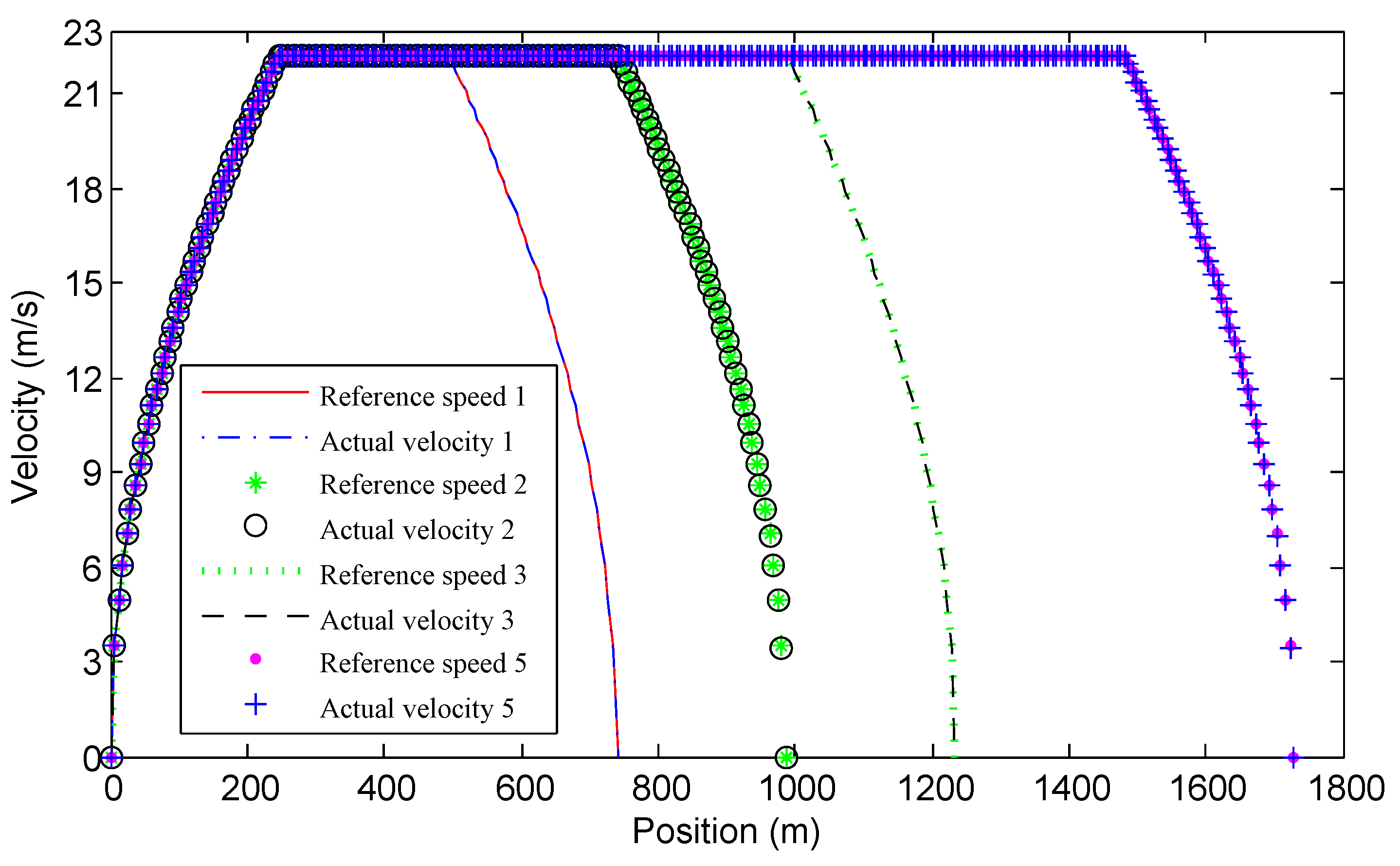
Figure 6.
The comparison of the numerical solution with the analytical solution. (a) ; (b) ; (c) .
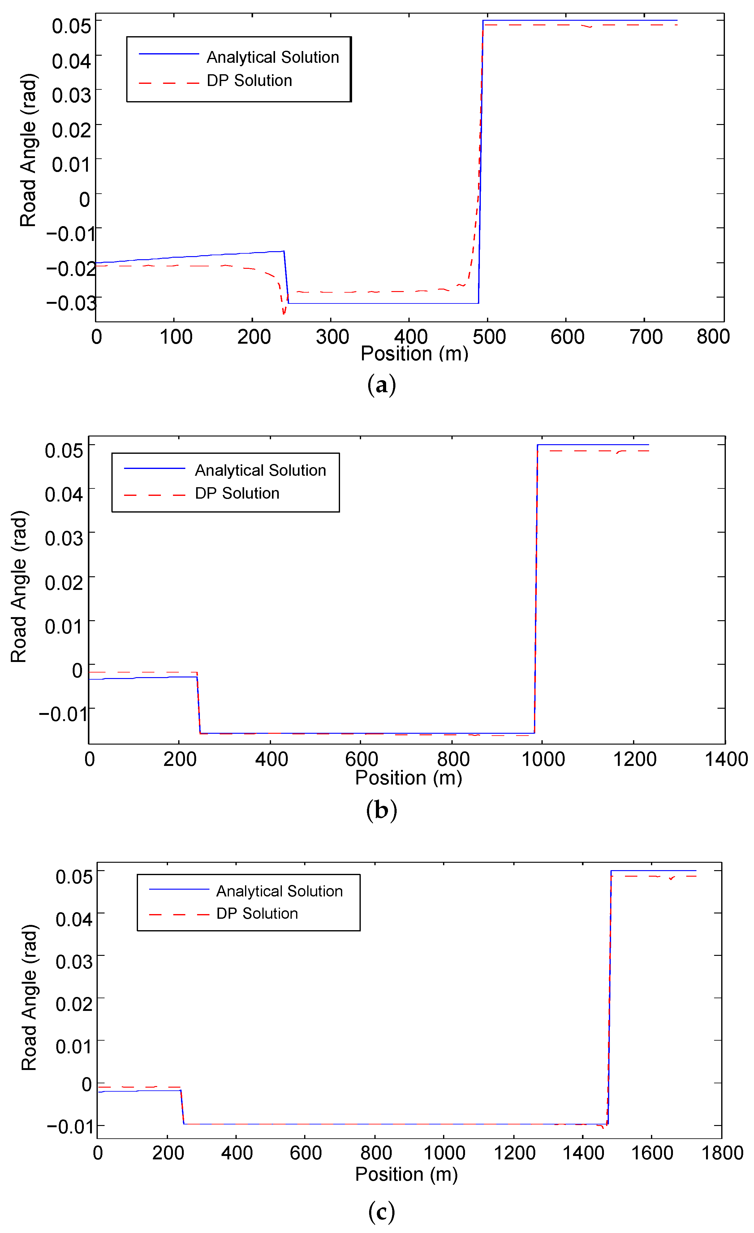
Figure 7.
The optimal and the symmetric roads. (a) The comparison of the optimal and the symmetric road grade profiles; (b) The comparison of the optimal and the symmetric road height profiles.
Figure 7.
The optimal and the symmetric roads. (a) The comparison of the optimal and the symmetric road grade profiles; (b) The comparison of the optimal and the symmetric road height profiles.
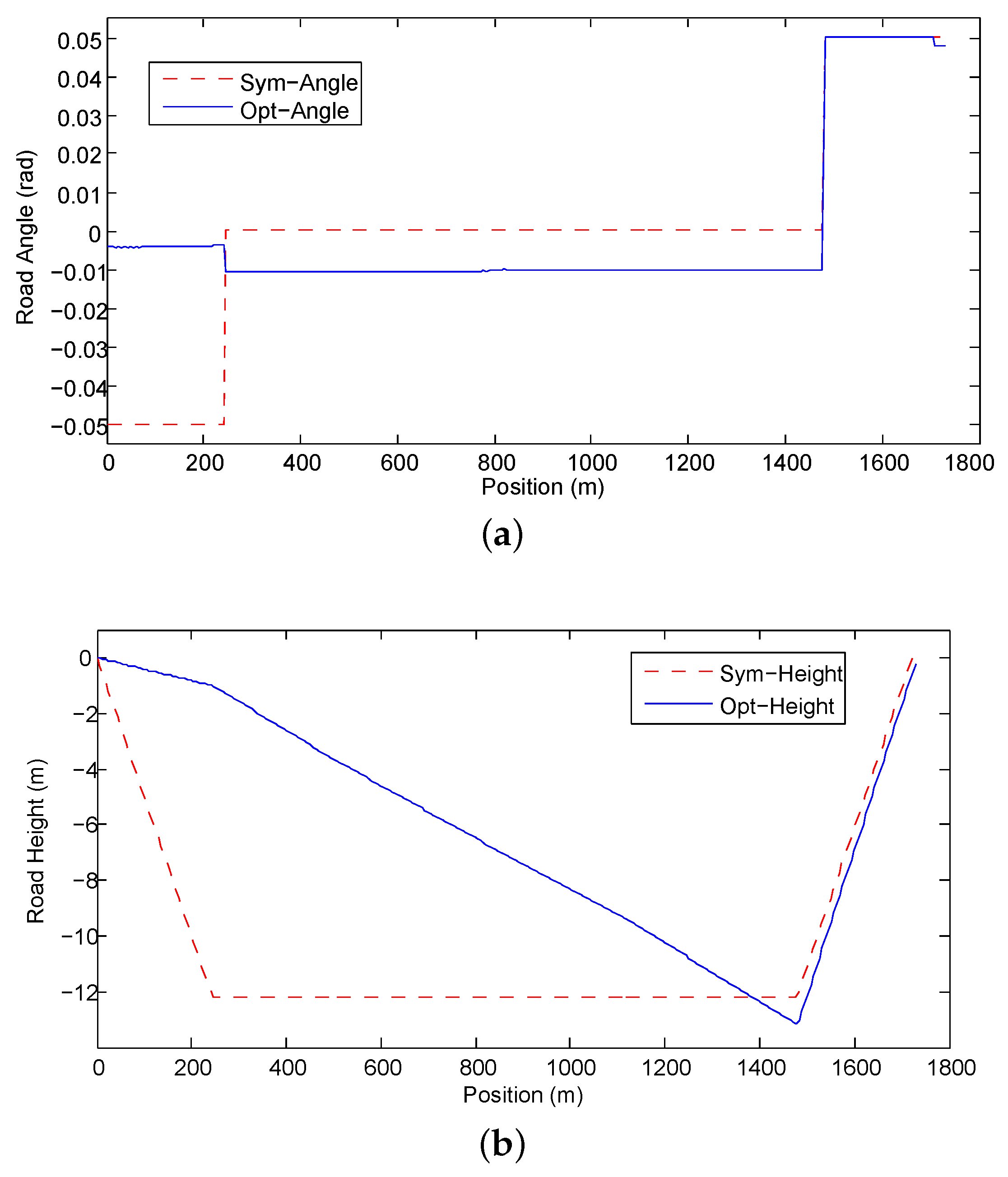
Figure 8.
Weight probability distribution is consistent with the assumption.

Figure 9.
Normal distribution.

Figure 10.
Exponential distribution.

Figure 11.
Uniform distribution.

Figure 12.
Lots of trucks and less of light vehicles.
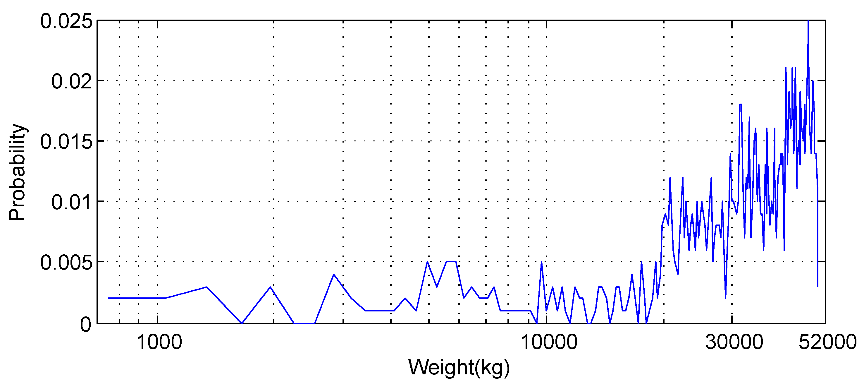
Figure 13.
The energy reduction of optimal road compared with flat road.

Figure 14.
The energy reduction of optimal road compared with symmetric road.

Figure 15.
The vehicles stop at half the distance.

Figure 16.
The vehicles stop at the uphill.

Figure 17.
The comparison of the road grade.

Figure 18.
The comparison of mean traction force for vehicles.


Table 1.
RMSE, normalized RMSE and maximal deviation of speed.
| Value of l | RMSE | Normalized RMSE (%) | Maximal Deviation (m/s) 1 |
|---|---|---|---|
1 The column shows the maximal absolute deviation between the reference and the actual speeds.
Table 2.
Comparison of energy consumptions.
| Value of l | Energy (J) | Reduction Percentage (%) | |||
|---|---|---|---|---|---|
| Flat Road | Symmetric Road | Optimal Road | Opt vs. Sym | Opt vs. Flat | |
| 0.52 | 32.6 | ||||
| 0.53 | 27.1 | ||||
| 0.43 | 23.1 | ||||
| 0.32 | 17.8 | ||||
Table 3.
Comparison of DP and PMP solutions.
| Value of l | Energy (J) | Relative Deviation (%) 1 | |
|---|---|---|---|
| DP Solution | Analytical Solution | ||
| 0.45 | |||
| 0.37 | |||
| 0.31 | |||
1 The column is calculated by the following equation: .
Table 4.
Comparison of traveling time.
| Value of l | Road | Distance (m) | Traveling Time (s) | Percentage of Increase (%) |
|---|---|---|---|---|
| Optimal Road by DP | 740.9390 | 52.7924 | 2.41 | |
| Optimal Road by PMP | 740.9486 | 52.6957 | 2.22 | |
| Symmetric Road | 740.1393 | 52.8091 | 2.44 | |
| Flat Road | 740.7407 | 51.5492 | – | |
| Optimal Road by DP | 1234.7076 | 74.8885 | 1.70 | |
| Optimal Road by PMP | 1234.7017 | 74.7725 | 1.55 | |
| Symmetric Road | 1233.9665 | 75.0313 | 1.90 | |
| Flat Road | 1234.5679 | 73.6343 | – | |
| Optimal Road by DP | 1728.4989 | 96.9720 | 1.31 | |
| Optimal Road by PMP | 1728.4945 | 96.8560 | 1.19 | |
| Symmetric Road | 1727.7936 | 97.2535 | 1.60 | |
| Flat Road | 1728.3951 | 95.7193 | – |
The column shows the percentage of increase of the traveling time for different road compared with the flat road.
Table 5.
Different parameters.
| Weight (kg) | Probability | |||
|---|---|---|---|---|
| 750 | 0.05 | 1.8000 | 0.3000 | 0.0100 |
| 1000 | 0.2 | 1.8546 | 0.3017 | 0.0100 |
| 1500 | 0.2 | 1.9636 | 0.3052 | 0.0099 |
| 2000 | 0.1 | 2.0732 | 0.3086 | 0.0099 |
| 5000 | 0.1 | 2.7290 | 0.3292 | 0.0096 |
| 8000 | 0.1 | 3.3848 | 0.3499 | 0.0093 |
| 10,000 | 0.1 | 3.8220 | 0.3636 | 0.0091 |
| 20,000 | 0.05 | 6.0080 | 0.4324 | 0.0080 |
| 30,000 | 0.05 | 8.1940 | 0.5012 | 0.0070 |
| 40,000 | 0.05 | 10.380 | 0.5700 | 0.0060 |
Table 6.
Comparison of simulation results (weight probability distribution is consistent with the assumption).
Table 6.
Comparison of simulation results (weight probability distribution is consistent with the assumption).
| Number of Vehicles | Road | Mean Average Energy (J) | Standard Deviation (J) | Reduction Percentage (%) |
|---|---|---|---|---|
| 1000 | Flat Road | 31.68 | ||
| Symmetric Road | 4.46 | |||
| Optimal Road | - | |||
| 10,000 | Flat Road | 31.67 | ||
| Symmetric Road | 4.46 | |||
| Optimal Road | - | |||
| 100,000 | Flat Road | 653.62 | 31.66 | |
| Symmetric Road | 991.13 | 4.46 | ||
| Optimal Road | 681.50 | - |
The reduction percentage is calculated from the mean values.
Table 7.
Standard deviation of reduction percentage.
| Number of Vehicles | Comparison | Standard Deviations of Reduction Percentages (%) | |||
|---|---|---|---|---|---|
| Normal | Exponential | Uniform | Lots of Trucks | ||
| 1000 | Opt vs. Flat | 0.05 | 0.122 | 0.036 | 0.0071 |
| Opt vs. Sym | 0.0084 | 0.022 | 0.0076 | 0.0095 | |
| 10,000 | Opt vs. Flat | 0.014 | 0.037 | 0.018 | 0.0018 |
| Opt vs. Sym | 0.0024 | 0.0066 | 0.0025 | 0.0095 | |
| 100,000 | Opt vs. Flat | 0.0035 | 0.009 | 0.0039 | 0.00053 |
| Opt vs. Sym | 0.00054 | 0.0016 | 0.00081 | 0.00081 | |
Table 8.
Simulation results (the vehicles stop at half the distance).
| Number of Vehicles | Road | Mean Average Energy (J) | Standard Deviation (J) | Reduction Percentage (%) |
|---|---|---|---|---|
| 1000 | Flat Road | 16.88 | ||
| Symmetric Road | ||||
| Optimal Road | - | |||
| 10,000 | Flat Road | 16.89 | ||
| Symmetric Road | ||||
| Optimal Road | - | |||
| 100,000 | Flat Road | 990.5073 | 16.89 | |
| Symmetric Road | ||||
| Optimal Road | 959.7524 | - |
Table 9.
Simulation results (the vehicles stop at uphill).
| Number of Vehicles | Road | Mean Average Energy (J) | Standard Deviation (J) | Reduction Percentage (%) |
|---|---|---|---|---|
| 1000 | Flat Road | 19.17 | ||
| Symmetric Road | 0.32 | |||
| Optimal Road | - | |||
| 10,000 | Flat Road | 19.18 | ||
| Symmetric Road | 0.38 | |||
| Optimal Road | - | |||
| 100,000 | Flat Road | 939.5625 | 19.17 | |
| Symmetric Road | 0.33 | |||
| Optimal Road | 923.0986 | - |
Table 10.
The comparison of energy consumption for different distances.
| Distance (km) | Mean Average Energy (J) | Standard Deviation (J) | Reduction Percentage (%) | ||
|---|---|---|---|---|---|
| Opt | Sym | Opt | Sym | ||
| 1.7 | |||||
| 5 | |||||
| 10 | |||||
| 20 | 0.01 | ||||
© 2017 by the authors. Licensee MDPI, Basel, Switzerland. This article is an open access article distributed under the terms and conditions of the Creative Commons Attribution (CC BY) license (http://creativecommons.org/licenses/by/4.0/).
Share and Cite
MDPI and ACS Style
Liu, J.; Feng, L.; Li, Z. The Optimal Road Grade Design for Minimizing Ground Vehicle Energy Consumption. Energies 2017, 10, 700. https://doi.org/10.3390/en10050700
AMA Style
Liu J, Feng L, Li Z. The Optimal Road Grade Design for Minimizing Ground Vehicle Energy Consumption. Energies. 2017; 10(5):700. https://doi.org/10.3390/en10050700
Chicago/Turabian StyleLiu, Junhui, Lei Feng, and Zhiwu Li. 2017. "The Optimal Road Grade Design for Minimizing Ground Vehicle Energy Consumption" Energies 10, no. 5: 700. https://doi.org/10.3390/en10050700
Note that from the first issue of 2016, this journal uses article numbers instead of page numbers. See further details here.