
A Numerical Study on the Impact of Grouting Material on Borehole Heat Exchangers Performance in Aquifers


1
Civil and Environmental Engineering Department, Politecnico di Milano, P.zza L. da Vinci 32, Milano 20133, Italy
2
Energy Department, Politecnico di Milano, via Lambruschini 4, Milano 20156, Italy
*
Author to whom correspondence should be addressed.
Energies 2017, 10(5), 703; https://doi.org/10.3390/en10050703
Submission received: 24 March 2017
/
Revised: 11 May 2017
/
Accepted: 12 May 2017
/
Published: 17 May 2017
(This article belongs to the Special Issue Low Enthalpy Geothermal Energy)
Abstract
:U-pipes for ground source heat pump (GSHP) installations are generally inserted in vertical boreholes back-filled with pumpable grouts. Grout thermal conductivity is a crucial parameter, dominating the borehole thermal resistance and impacting the heat exchanger efficiency. In order to seal the borehole and prevent leakages of the heat carrier fluid, grouting materials are also hydraulically impermeable, so that groundwater flow inside the borehole is inhibited. The influence of groundwater flow on the borehole heat exchangers (BHE) performance has recently been highlighted by several authors. However groundwater impact and grouting materials influence are usually evaluated separately, disregarding any combined effect. Therefore simulation is used to investigate the role of the thermal and hydraulic conductivities of the grout when the BHE operates in an aquifer with a relevant groundwater flow. Here 3 main cases for a single U-pipe in a sandy aquifer are compared. In Case 1 the borehole is back-filled with the surrounding soil formation, while a thermally enhanced grout and a low thermal conductivity grout are considered in Case 2 and Case 3 respectively. Simulations are carried out maintaining the inlet temperature constant in order to reproduce the yearly operation of the GSHP system. For each of the 3 cases three different groundwater flow velocities are considered. The results show that a high thermal conductivity grout further enhances the effects of a significant groundwater flow. The conditions when neglecting the grout material in the numerical model does not lead to relevant errors are also identified.
1. Introduction
Borehole heat exchanger (BHE) technology is growing on a worldwide scale. Ground source heat pump (GSHP) systems are used increasingly because they are among the cleanest and most energy efficient heating/cooling systems for buildings. Furthermore this technology is being applied widely, not only in civil buildings, but also in agricultural and zoo-technical facilities [1]. From the hydrogeological point of view, one of the most important aspects in the use of GSHP systems is the forecast and control of the temperature in aquifers and the development of the heat perturbation in groundwater, often considered as a contaminant plume in some environmental regulations. From here, the need arises to simulate, through mathematical models, the GSHP systems in order to evaluate the impact of temperatures in the subsoil [2,3].
Some of the most used hydrogeological computer codes, for instance MT3DMS [4] or FEFLOW [5], are suitable for reproducing heat transfer between BHE and aquifer and have been recently used to simulate BHE operation in different hydrogeological settings. In previous studies [6], the authors demonstrated that MT3DMS can be used to predict the thermal impact and the energy performance of BHE systems with a good accuracy, fully simulating the U-pipe geometry and the heat carrier fluid. The model predictions were compared to some well-known analytical solutions, producing a very good agreement in the purely conductive case and a good agreement for a wide range of Darcy velocities.
The energy performance of GSHPs strongly depends on the heat transfer process between the BHEs and the ground. The BHE, which often consists of single or double U-shaped pipes inserted in a borehole back-filled with grout, is characterized by an effective thermal resistance Rbh [7] related to the temperature drop between the average fluid temperature and the BHE wall. The grout provides a heat transfer medium between the heat exchanger and the surrounding formation and prevents contamination in case of leakage of the anti-freeze circulating fluid. Grout thermal conductivity is known as a crucial parameter, dominating the borehole thermal resistance [8,9] and impacting the heat exchanger efficiency [10,11,12,13]. Therefore so-called thermally enhanced grouts are being developed and investigated since the late 90’s [14,15,16]. Clearly a grouting material with low thermal conductivity increases the borehole thermal resistance, although the latter closely depends also on the spacing between the pipes [17,18,19]. Although these studies are related to the use of thermally enhanced grouts, it remains unclear how much these ones can improve long-term BHE performance. Dehkordy and Schincariol [20] indicated that a thermally enhanced grout (λg = 3 W·m−1 K−1) increases heat extraction by more than 10% compared to a grout with poor thermal conductivity (λg = 1 W·m−1 K−1). However, this influence has to be compared to that of the ground thermal conductivity, which can play a more important role in increasing or reducing BHE performance. Ghasemi-Fare and Basu [21] showed that the soil thermal conductivity has a much larger impact on the long-term energy performance of an energy pile than the pile thermal conductivity. In Delaleux et al. [22], an enhancement of the grout thermal conductivity was chosen as the best way to improve the overall exchanger performance; Jun et al. [23] evaluated the grout conductivity influence on the heat transfer length and on the thermal resistance of borehole and soil. Finally, Lee et al. [24] stated that an increase in the thermal conductivity of backfilling grouts leads to considerable reduction in the installation cost of a ground heat exchanger by shortening the required bore length.
While most studies focused on the thermal properties of the grout, it is important to keep in mind that grout is also characterized by a very low hydraulic conductivity and this property can play a role in BHE performance in subsoils with a significant groundwater flow. The impact of groundwater flow on the ground heat exchangers operation and performance in the short and long term was recently investigated and highlighted by several authors [12,13,25,26,27,28]. As far as groundwater-influenced Thermal Response Tests are concerned, Wagner et al. [29] pointed out that the discontinuity in the hydraulic properties passing from the grout to the surrounding ground may result in a different borehole wall temperature affecting the TRT interpretation. However, to the best of the authors’ knowledge, whenever a sensitivity analysis of the BHE efficiency to relevant parameters is performed [10,13,30,31], groundwater impact and grouting materials influence are evaluated separately, disregarding any combined effect.
As long as conduction is the only heat transfer mechanism in the surrounding ground, the low hydraulic conductivity of the grout has marginal impact on the borehole thermal performance. In turn, when a significant groundwater flow is present, the question arises whether hindering advection in the borehole results in a penalty. Therefore in this paper finite-difference numerical simulations investigate the role of the grouting material thermal and hydraulic conductivities when the borehole heat exchanger operates in an aquifer with a relevant groundwater flow. A single U-pipe borehole in a sandy aquifer is simulated as in the previous study by the authors [6], where however the surrounding soil formation was assumed as back-filling material for the borehole. A comparison is then carried out among the base case (Case 1), where the borehole is back-filled with the surrounding soil formation, and the cases where thermally enhanced grout (Case 2) and poor grout are used (Case 3).
Simulations are carried out maintaining the inlet temperature constant in order to reproduce the yearly operation of the GSHP system. Then the effect of the grouting material is assessed comparing the models results. Three groundwater flow velocities are simulated: the null-velocity (i.e., purely conductive condition), i.e., Case a, Darcy velocity equal to 10−6 m/s, i.e., Case b and 10−5 m/s, i.e., Case c. A list of parameters and symbols used in the paper is shown in Nomenclature.
2. Heat and Mass Transport Equations
In this section the heat and mass transport equations at the basis of the numerical modelling are briefly introduced. Firstly, the analogy between solute transport and heat transport, at the basis of the use of MT3DMS, is shown. Then heat and mass transport equation is put in a form that allows to identify the physical quantities required as inputs by the tool.
Indeed MT3DMS is a modular three-dimensional multispecies transport model for the simulation of advection, dispersion and chemical reactions of contaminants in groundwater systems [4] and represents the evolution of MT3D. MT3DMS can be used to simulate concentration changes in miscible contaminants in groundwater through advection, dispersion, diffusion and some basic chemical reactions, with various types of boundary conditions and external sources or sinks. MT3DMS can accommodate very general spatial discretization schemes and transport boundary conditions. MT3DMS is designed for use with any block-centered finite-difference flow model, such as the U.S. Geological Survey code named MODFLOW [32,33].
The partial differential equation describing the fate and transport of contaminants of species k in three-dimensional, transient groundwater flow systems, disregarding chemical reactions, can be written as follows [4]:
where:
is the bulk density and:
Kd is the distribution coefficient. Other symbols and parameters are listed in Nomenclature.
Even though MT3DMS was designed to simulate solutes transport, thanks to analogies between the heat transport and solute transport equation, Equation (1) can be rewritten considering temperature as one of the chemical species transported. Nevertheless, as the energy is transported and stored both by the fluid and the solid, some adaptations are required [34], as explained below.
Storage: in Equation (1) the left term accounts for changes in solute storage in an aquifer matrix due to sorption processes. As heat is stored both in solid and liquid phase, both the specific heat capacity cps and cpw have to be considered on the left side. Energy stored in the solid depends on temperature, solid volume, heat capacity and density: . Similarly energy stored in the fluid phase is given by: .
Thermal equilibrium was assumed to be between the solid and the fluid phase. Then the storage term in the heat transport equation can be written as:
Advection: considering the advection process for heat transport, it is necessary to relate the temperature of the flowing water to the energy stored in the fluid. The energy can be calculated multiplying temperature by water density and specific heat capacity. As vi is the volumetric flow rate per unit area [(m3/s)/m2], multiplying it by gives the mass flow rate per unit area which, when multiplied by water temperature and specific heat capacity, gives the advective heat flux in the flowing water: .
Therefore, the advection term can be rewritten as:
Diffusion-Dispersion: in solute groundwater transport, contaminant movement can be considered essentially limited to the liquid phase, whereas energy is also carried through the solid by the conduction process. This means that the diffusion process cannot be neglected for heat transport. As stated by Fourier’s law, assuming an isotropic medium, the heat flux by conduction is given by:
For a saturated porous medium, two different thermal conductivity values need to be used in the right term that takes into account diffusion-dispersion processes, namely λs for solid phase and λw for liquid phase, as well as an effective thermal conductivity:
Then a last adaptation is necessary for the dispersion transport because, similarly to advective transport, it is needed to relate the temperature of the “dispersed flowing” water to the energy stored in the fluid, which depends on density and specific heat capacity. The term in Equation (1) is thus replaced by:
Source/Sink: the last term in Equation (1) represents the source or sink that adds or extracts solute mass from the system. Again for heat transport it is needed in order to take into account the energy stored in the fluid. Hence the new term is:
Consequently, taking into account all the modifications described above, the heat transport equation can be written as [34]:
Note that if there is no groundwater flow, the pore velocity is null, so the advection and dispersion terms can be erased. Based on these hypothesis Equation (10) can be rewritten in the form of Fourier’s equation:
where π is the energy source/sink term (W/m3).
Considering Equation (10), by dividing all the terms by the following was obtained:
By introducing the bulk density as in Equation (2), the distribution coefficient Kd as in Equation (3) and the diffusion coefficient D* as in the following equation:
Equation (12) can be rewritten in a form where the input parameters necessary for MT3DMS implementation are shown:
In this study, Equations (11) or (14) are applied in every portion of the domain that is composed of a porous saturated medium (the sandy aquifer), a solid (the pipe) and a fluid (the heat carrier fluid into the U-pipe). The input parameters in Equation (14) are varied in each part of the domain according to its properties.
3. Model Implementation
The case study refers to a typical BHE, consisting of a 100 m polyethylene U-pipe with an internal diameter of 0.04 m and a pipe-to-pipe centerline distance of 0.06 m, as in Angelotti et al. [6]. The U-pipe is a 200 m deep saturated sandy aquifer, assumed homogeneous with an hydraulic conductivity of 2 × 10⁻⁴ m/s, a frequent value detected in the Po Plain area [35,36]. A simple three-dimensional model is implemented (Figure 1), in which active cells are assigned properties representing the aquifer and the pipe where the heat carrier fluid is assumed to circulate. Preliminary considerations demonstrated the importance in describing the entire U-pipe geometry [37] and considering the thermal resistance of the plastic pipe, despite the fact that this could require a significant computational effort. An initial undisturbed aquifer temperature (Tg0) equal to 11.8 °C, representative of the yearly average air temperature in Milan, Northern Italy, is set for the entire domain as boundary condition (Constant Concentration, i.e., Dirichlet condition) on the left and right sides of the model. The pipe is represented with a square section, whose size is derived from the assumption of conserving the total thermal resistance per unit length between the heat carrier fluid and the surrounding ground, as shown more in detail in Angelotti et al. [26]. It was found that a circular pipe with an internal diameter of 4 cm is equivalent to a square pipe with a side (L) of 3.36 cm. The polyethylene thickness (sp) is equal to 0.37 cm and is representative of real commonly used U-pipes. This representation requires a strong grid refinement in MODFLOW. The cells strictly representing U-pipes and the drilled hole where they are inserted, smoothly varied from 0.37 cm to 0.66 cm maintaining constant the total thermal resistance between circular and square geometry and the classical 6 cm distance between the two center of pipes. Row and column widths range from 0.0037 to 10 m; layers have variable thickness ranging from 0.0037 to 25 m. The horizontal model domain was varied according to the groundwater velocity simulated, because the higher is the flow velocity, the more extended should be the horizontal domain in order to distance the down-gradient constant head boundary condition. The vertical model domain is independent from groundwater flow velocity and is divided in 18 layers. In order to hydraulically isolate the cells representing the pipe from the aquifer, the MODFLOW Package Horizontal Flow Barrier (HFB) is assigned to the polyethylene pipe walls (kp = 10−21 m/s). The parameters assigned to the aquifer, borehole and pipe cells are set with reference to [34]. The thermal and hydrogeological properties of the porous medium and of the pipe wall are listed respectively in Table 1 and Table 2. Constant Head (i.e., Dirichlet condition) H = 1 m is assigned in layer 1 to the left side cells representing the entrance of the U-pipe, while h = 0.508 m is set for the right side cells representing the exit of the U-pipe in order to correctly simulate the heat carrier fluid flow rate inside the pipe (1000 kg/h) that represents the usual operating rate. Observation points are located downstream the BHE along the flow line indicated in Figure 1. The solver algorithm adopted in the calculation is the Jacobi solver, used for a finite difference solution scheme. The number of stress periods is variable according to the different simulated cases. For instance, a stress period equal to 183 days (representing the winter period) was divided into 12 simulations. In any stress period, the transient time step was set equal to a maximum of 0.024 days (34 min).
In accordance with Hecht-Mendez et al. [38], previous simulations carried out with this model [6] demonstrated that MT3DMS can be used to predict the thermal impact and the energy performance of such systems with good accuracy, comprehensively simulating the U-pipe geometry and the heat carrier fluid. Details about the model validation under different groundwater flow velocities can be found in Angelotti et al. [6].
Grout Implementation
The previously validated model [6] is used here to evaluate the influence of the back-filling grout on the seasonal energy performance and on the temperature distribution in the subsoil. For this reason three main cases are compared (Table 3), differing for the back-filling material inserted in the 12.5 cm diameter borehole:
- (1)
- the surrounding aquifer material;
- (2)
- a thermally enhanced grout with a thermal conductivity equal to the surrounding soil;
- (3)
- a poor grout with a low thermal conductivity.
In Table 3 the borehole thermal resistance Rbh calculated by means of GLHEPRO tool [39] in the 3 cases is also reported for the sake of comparison (Figure 2).
Firstly, it is worth clarifying that Case 1 is mainly a theoretical case used here as reference, since backfilling the borehole with a proper grouting material is the common practice in most countries and in some of them, e.g., Germany, the grouting material has to comply with a specific maximum hydraulic conductivity. Therefore even though the hydraulic conductivity value of the grout in Case 1 would not be realistic for a grouting material, it is adopted here just in order to investigate the influence of the hydraulic conductivity. Actually the high thermal conductivity grout Case 2 differs from the base Case 1 only because of the lower hydraulic conductivity of the grout. The grout thermal conductivity value (2.3 W/mK) of Case 2 can be achieved by mixing water and a specific commercial grout powder, called Thermoplast PLUS® (GTS well components S.n.c., San Benedetto Po, Italy), with a ratio 1:1.12. Having the same thermal conductivity, the borehole thermal resistance Rbh of Case 2 is the same as the base case. Therefore it can be argued that, as long as groundwater flow is negligible, the energy performance will be similar. Then it is interesting to investigate what happens at increasing Darcy velocity.
The low thermal conductivity grout Case 3 instead differs from the base Case 1 due to both a lower hydraulic and a lower thermal conductivity. The low value of thermal conductivity (0.7 W/mK) of this back-filling material corresponds to neat cement grouts [40]. A worse energy performance at null Darcy velocity is then expected because of the higher BHE thermal resistance Rbh (+151%). However, when a significant Darcy flow in the aquifer is present, it is interesting to investigate how distant are the BHE performances depending on the kind of grout adopted. For this reason the effect of the grouting material is assessed comparing the models. Different Darcy velocities are considered: (a) 0 m/s, (b) 10−6 m/s (8.6 cm/day) and (c) 10−5 m/s (86.0 cm/day), as shown again in Table 3. The Case a corresponds to an extreme situation where the hydraulic gradient is nearly null (horizontal water table). The previous study by the authors Angelotti et al. [6] demonstrated that at a Darcy velocity equal to 10−7 m/s the geothermal system behaviour is very similar to null velocity, therefore the minimum velocity adopted here is 10−6 m/s. Thus Cases b and c are generally representative of the velocities in alluvial sediments. Simulations are carried out maintaining the inlet fluid temperature constant at 1 °C for 6 months in order to reproduce, in a simplified way, the winter operation of the GSHP system.
4. Simulation Results
Simulations of Cases 1, 2 and 3 are compared at variable Darcy velocity (a, b, c). The energy exchanged by the BHE during the winter operation is calculated as:
and shown in Table 4 together with the percentage differences related to Case 1 for the same Darcy velocity. At null groundwater velocity the seasonal energy performance of the BHE is very similar between the base case (Case 1a) and the high thermal conductivity grout case (Case 2a), as thermal conductivity of the material surrounding the U-pipe is the same. As shown in Table 4 at a velocity equal to 10−5 m/s the seasonal energy exchanged with the high conductivity grout (Case 2c) becomes slightly smaller (−1.3%) than the Case 1c. In the latter case, back-filling with the surrounding ground means promoting advection around the pipe and thus slightly increasing the exchanged energy. However it can be argued that the differences in the seasonal exchanged energy between the base case and the high thermal conductivity grout case, at every velocity, are in the order of magnitude of the numerical accuracy.
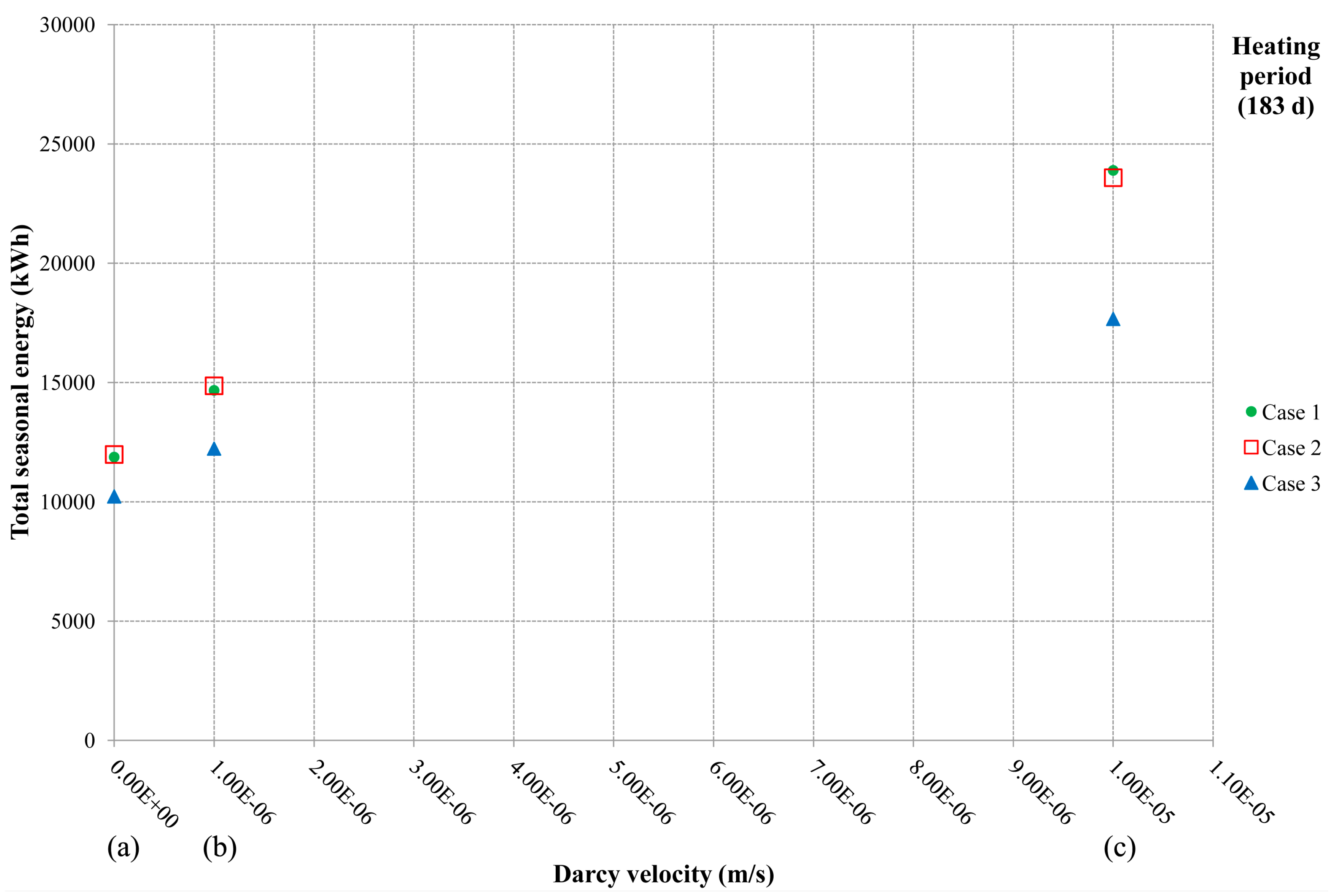
As expected at null groundwater velocity, the energy performance of the low thermal conductivity grout (Case 3a) is worse (−13.9%) than the base case (Case 1a). Further, it becomes even worse (−26.1%) at high groundwater velocity (Case 3c vs. 1c). Similar results are found comparing the low thermal conductivity grout cases (3a, 3b and 3c) with the high thermal conductivity (Cases 2a, 2b and 2c respectively). This is also shown in Figure 3, that represents the total seasonal energy extracted from the ground versus Darcy velocity for different grout types (namely cases 1, 2 and 3), and in Figure 4, where the heat rate extracted from the ground for different Darcy velocities is plotted versus the time from the beginning of the winter season.
As shown in Figure 3, the influence of Darcy velocity on the BHE energy performance is more significant in Cases 1 and 2, i.e., at relatively low borehole thermal resistance Rbh. Actually, compared to the null groundwater velocity case, a Darcy velocity equal to 10−5 m/s increases seasonal energy by 101% (Case 1c), 97% (Case 2c) and 73% (Case 3c).
The usefulness of the thermal network analysis to predict borehole heat exchangers energy performance was shown by several authors, e.g., Zeng et al. [8]. Even here, a semi-quantitative explanation of these outcomes can be obtained with a simple thermal network modeling of the heat transfer between the heat carrier fluid in the U-pipe and the ground at the end of the winter season, when a steady state has almost been reached (as shown in Figure 4). In such condition the specific heat rate exchanged by the BHE can be expressed as:
where the ground thermal resistance Rg is expected to decrease at increasing Darcy velocity (vi) due to the contribution of the advection. At the same time:
where z is the borehole depth. Combining the two equations we obtain:
Therefore, given that the fluid inlet temperature and the undisturbed ground temperature are the same in all the cases, the resulting heat rate is inversely proportional to the total thermal resistance:
Extracting the heat flow rate at the end of the winter season from Figure 4 and using the borehole resistance Rbh calculated from GLHEPRO tool in Table 3, the ground resistance Rg at each velocity can be derived from Equation (18).
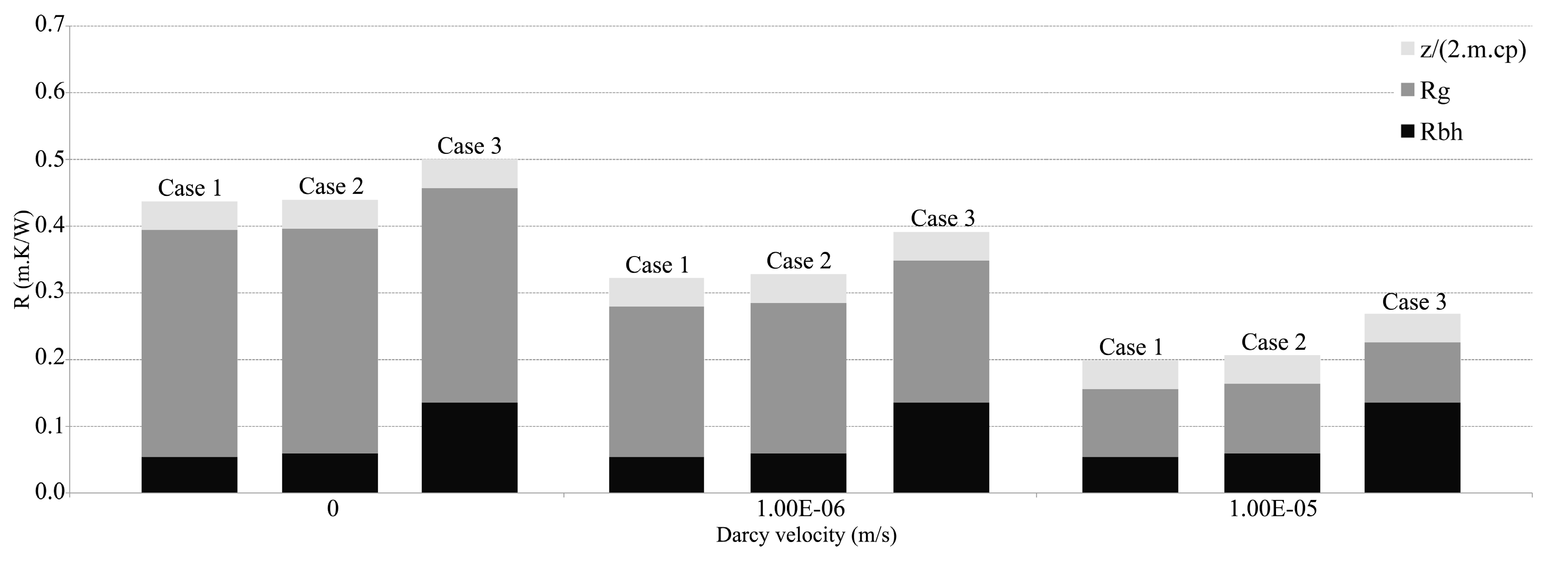
The composition of the total thermal resistance in Case 1, Case 2 and Case 3 is then shown in Figure 5. In each case it is evident that, as the Darcy velocity increases, the total thermal resistance decreases (e.g., Case 1c vs. 1a, −54.6%). Furthermore it is evident that for the low thermal conductivity grout Case 3 the total resistance is higher respect to the other two cases because of the relatively high value of the borehole thermal resistance, while the ground resistance Rg and the term do not seem to change for the three different cases. That means the higher the Rbh is, depending on the borehole grout, the less is the impact of the Rg decrease on the total thermal resistance variation (Case 3c vs. 3a, −46.4%).
The results obtained from the above simulations can be analyzed from different perspectives:
- From the modeling perspective, these results indicate that when the grout has a thermal conductivity equal or near to the surrounding ground, neglecting the grouting material in the numerical model does not lead to relevant errors, even at important Darcy velocities. On the contrary, when the grouting material has a poor thermal conductivity compared to the surrounding ground, it is necessary to represent the grout in the numerical model because neglecting it leads to significantly overestimate the BHE performance. Moreover, this study specifically shows that the overestimation increases with Darcy velocity.
- From the BHE design perspective, these results indicate that adopting a high thermal conductivity grout is even more important at high Darcy velocities, since it further enhances the benefits of the advective transport in the surrounding aquifer. Furthermore it arises that reducing the environmental risk of heat carrier fluid leakages by adopting a grout in the borehole does not affect significantly the BHE performances (see Table 4, the maximum seasonal energy decrease is −1.3%). The negligible decrease is due to the low hydraulic conductivity in the neighborhood of the pipes.
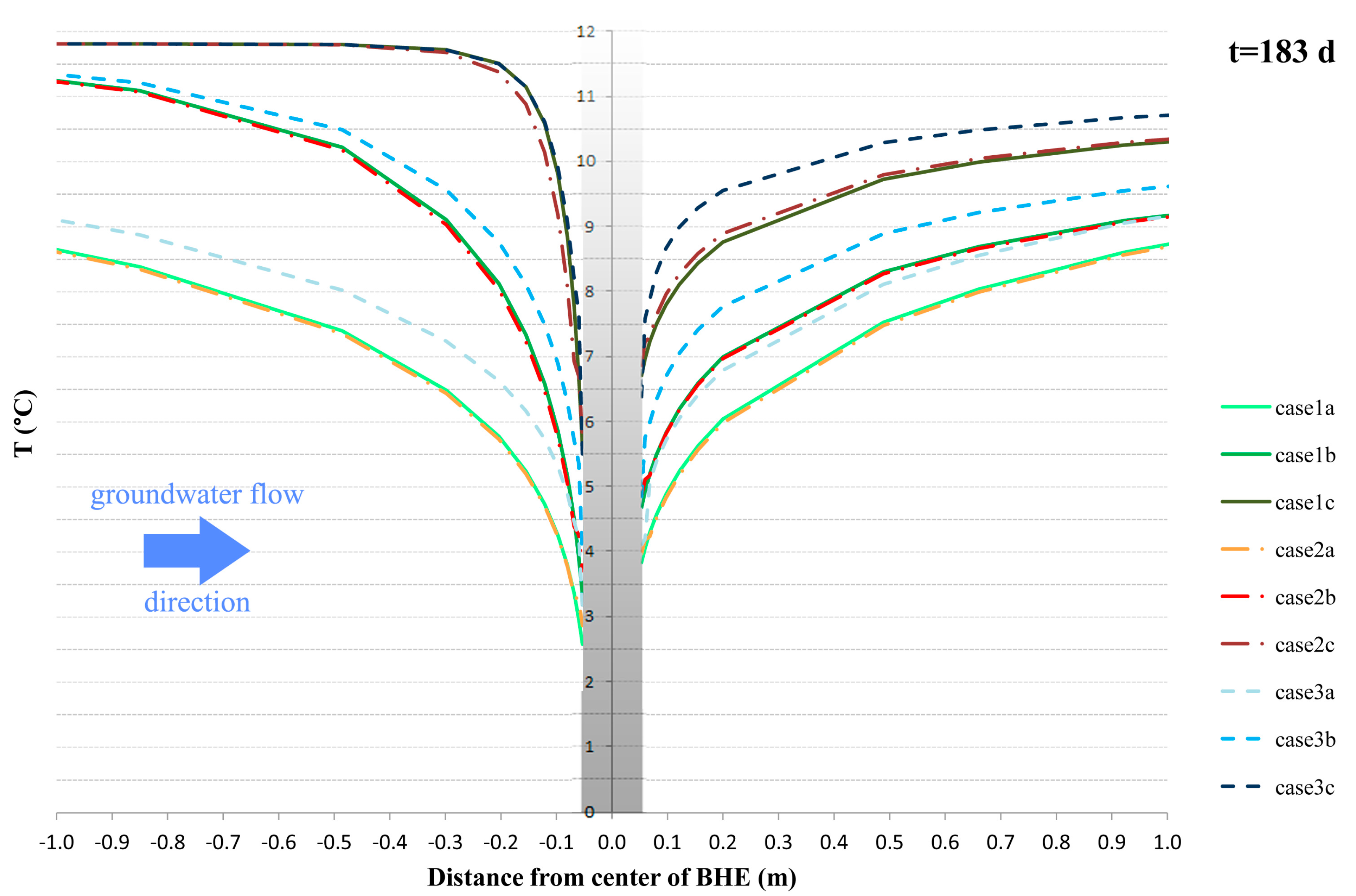
- From the environmental perspective it is interesting to assess the possible impact of the grout on the temperature distribution in the subsoil. The cold thermal perturbation generated in the aquifer at the end of the winter BHE operational period is then shown in Figure 6 for the three considered velocities and the three grouting cases. The Figure 6 shows the ground temperature distribution across the BHE along the longitudinal groundwater flow direction approximately at half the BHE depth. It is worth noting that, since in the model the inlet pipe is positioned exactly upstream while the outlet pipe is downstream, the curves are not symmetrical, even in the null velocity condition. The latter absence of symmetry was already remarked by several authors, e.g., Kramer et al. [41].
As expected, whatever the grouting material, when high groundwater velocity is simulated (10−5 m/s) the BHE cooling effect in the aquifer is less pronounced, i.e., a large advection component causes a lower environmental impact. No differences between thermal perturbations in Case 1 and Case 2 are observed for the null (a) and the moderate (b) Darcy velocities. Instead for the highest velocity (c) a slight difference in aquifer temperature can be noted: however such difference in the proximity of the borehole is always lower than 0.7 °C and becomes negligible beyond 20 cm from the center of the U-shaped pipe. Different from the other two is Case 3, which always shows higher temperature values in the subsoil for the three velocities. The temperature difference between the poor grout case and the other two reduces to less than 1 °C at about 1 m from the U-pipe downstream.
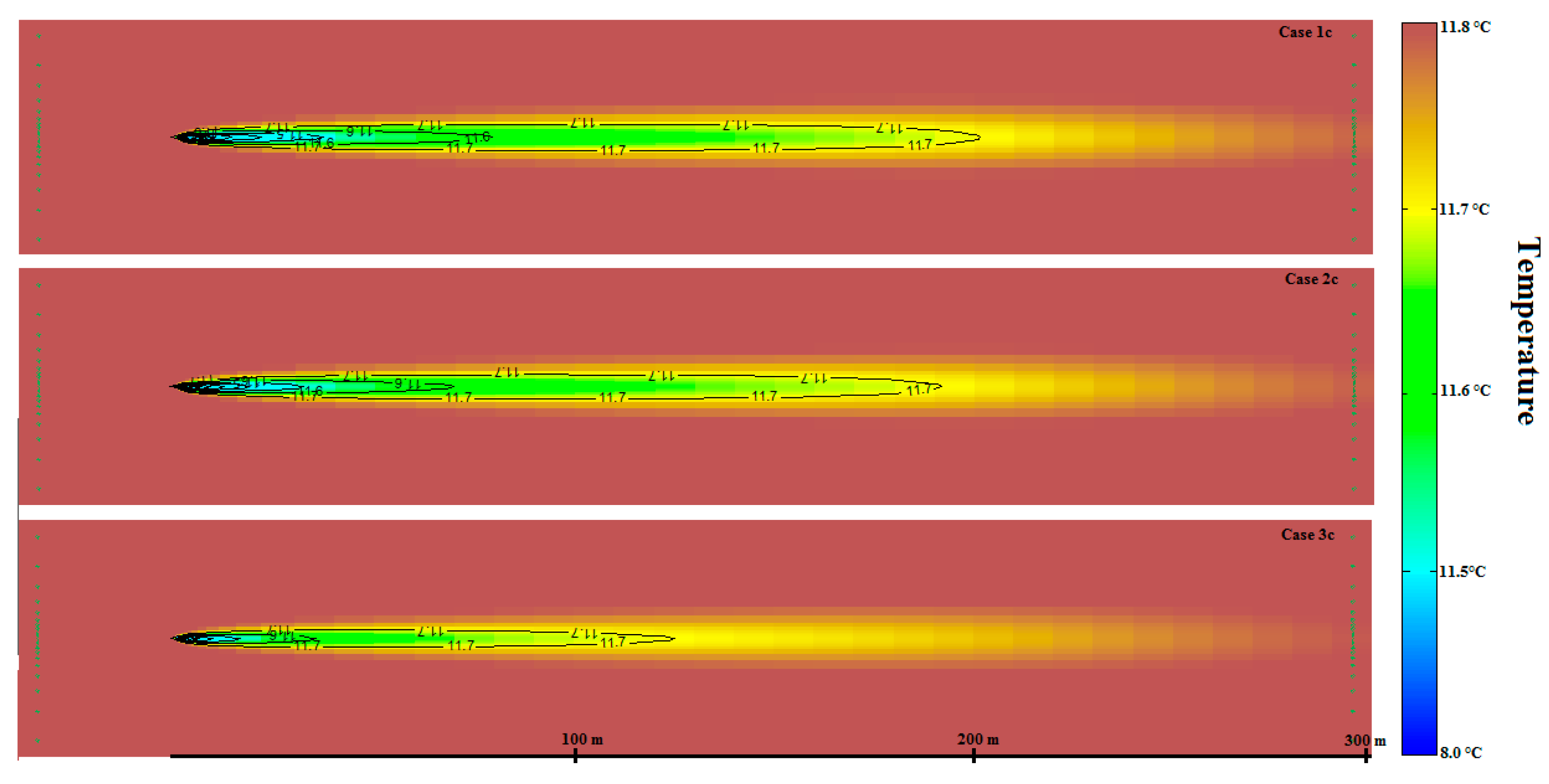
Considering the environmental point of view, these outcomes confirm that disregarding the grout in the model is a safe option, since it leads to slightly overestimate the BHE environmental impact. This result is also confirmed by the representation of the temperature perturbations in the plan view, reported in Figure 7, showing that in Case 1c the plume length (e.g., considering the isothermal line 11.7 °C) is always overestimated compared to Cases 2c and 3c. The plume length of the isothermal line 11.7 °C is extended to 200 m, 190 m and 125 m for Cases 1c, 2c and 3c respectively. One again the Case 3 with a poor grout shows the greatest differences compared to the other two cases.
5. Conclusions
In this paper the role of the grouting material for a BHE operating in an aquifer with a relevant groundwater flow is investigated by means of a finite-difference numerical model. The effect of the two kinds of grouting materials is assessed at variable Darcy velocities, both in terms of exchanged energy and temperature distribution in the subsoil. Adopting a thermally enhanced grout (Case 2) instead of back-filling with surrounding soil formation (Case 1) results in marginal variations in the exchanged energy both in conduction-dominated conditions (0 m/s and 10−6 m/s) and in the advection-dominated one (vi = 10−5 m/s). Furthermore, as far as temperature distribution in the subsoil is concerned, simulations reveal that the effect of the high thermal conductivity grout (Case 2) is negligible: there is only a minimal difference respect to back-filling with ground (Case 1) very near to the BHE (20 cm around the pipe) and mainly in the advective-dominated case.
In turn in the comparison between Case 1 and the low thermal conductivity grout (Case 3), appreciable differences have been noticed. At null groundwater velocity, the energy performance in Case 3 is worse than the Case 1 by 14%. Further, it becomes even worse at the highest groundwater velocity, since the higher the borehole thermal resistance, the lower the impact of the ground resistance decrease on the total thermal resistance between the thermal carrier fluid and the undisturbed ground. From the BHE design perspective, these results indicate that adopting a high conductivity grout is even more important at high Darcy flows, since it further enhances the benefits of the advective transport in the surrounding medium. Case 3 also shows higher temperature values in the subsoil for the three considered velocities, namely the BHE impact on the subsoil is lower in accordance to the lower heat exchange rate.
These results allow also to derive some considerations on the numerical modeling issue. When the grout has a thermal conductivity similar to the surrounding ground is not necessary to represent the grouting material in the numerical model, even at important Darcy velocity, namely the effect of the discontinuity in the hydraulic conductivity between the surrounding ground and the borehole is marginal. This is justified by the fact that the energy exchanges differences are negligible and aquifer temperature variations are slightly overestimated by the model that assumes the borehole is back-filled by surrounding formation. Differently, when the grouting material has a poor thermal conductivity compared to the surrounding ground, neglecting the grout in the numerical model leads to overestimate significantly the BHE performance. Moreover, the overestimation increases with Darcy flow. In this case it is recommended to fully represent the grout in the numerical model.
Author Contributions
All authors conceived and designed the methodology and discussed simulation results. Most of the results achieved in this study derive from Matteo Antelmi’s Ph.D. thesis. Luca Alberti supervised Antelmi’s Ph.D. thesis as an expert in the hydrogeology area and in groundwater numerical modeling; he also wrote the section of mathematical equations together with Adriana Angelotti, who was the co-supervisor of Antelmi’s Ph.D. thesis. She is an expert in energy engineering area and analysed the simulation results in aquifer in terms of BHE energy performance. Matteo Antelmi, being an expert in heat transport simulations by means of his Ph.D. thesis, run all simulations together with Ivana La Licata, who is an expert in the groundwater numerical modeling through MODFLOW code. Therefore, the following manuscript was written by the 4 authors in equal parts.
Conflicts of Interest
The authors declare no conflict of interest.
Nomenclature
| Symbol | Variable | Unit |
| BHE | Borehole Heat Exchanger | - |
| Cm, Cw, Cp | Volumetric heat capacity of the porous medium or water or pipe | J/(m3·K) |
| Ck | Dissolved mass concentration | kg/m3 |
| Cs | Concentration of the sources or sinks | kg/m3 |
| cps, cpw, cpf | Specific heat capacity of the solid or water or fluid | J/(kg·K) |
| D* | Molecular diffusion coefficient/Thermal diffusion coefficient | m2/s |
| Dij | Diffusion-dispersion tensor | m2/s |
| d, dp | Dispersivity coefficient of the porous medium or pipe | m |
| E | Exchanged energy by BHE | kWh |
| θ, θp | Volumetric water content of the porous medium or pipe | - |
| GSHP | Ground Source Heat Pump | - |
| H, h | Hydraulic head | m |
| km, kg, kp | Hydraulic conductivity of the porous medium or grout or pipe | m/s |
| Kd | Distribution coefficient | m3/kg |
| λm | Effective thermal conductivity of the porous medium | W/(m·K) |
| λg, λs, λw, λp | Thermal conductivity of the grout or solid or water or pipe | W/(m·K) |
| I | Identity tensor | - |
| L | Side of the pipe represented by square section | m |
| Mass flow rate at time i | kg/s | |
| π | Energy source/sink rate per unit volume | W/m3 |
| qi | Heat rate per unit length or specific heat rate | W/m |
| qs | Volumetric flow rate per unit volume of aquifer representing sources and sinks | (m3/s)/m2 |
| qt | Heat flux | W/m2 |
| Rbh, Rg | Borehole or ground thermal resistance per unit length | m·K/W |
| ρb | Porous medium bulk density | kg/m3 |
| ρs, ρw | Density of the solid material or water | kg/m3 |
| sp | Thickness of the pipe | m |
| T, Ts, Tg0 | Temperature, temperature of the source or undisturbed ground | K |
| Tfi, Tfo, Tfm | Inlet, outlet or average temperature of the heat carrier fluid | K |
| t | Time | s |
| vi | Groundwater Darcy velocity | m/s |
| xi, xj | Space coordinates along directions i and j | m |
| z | Borehole depth | m |
References
- Angelotti, A.; Alberti, L.; Antelmi, M.; Formentin, G.; Legrenzi, C. Zoo-technical application of ground source heat pumps: A pilot case study. In Proceedings of the 12th REHVA World Congress 2016 (CLIMA 2016), Aalborg, Denmark, 22–25 May 2016. [Google Scholar]
- Alcarez, M.; Garcìa-Gil, A.; Vázquez-Suñé, E.; Velasco, V. Advection and dispersion heat transport mechanisms in the quantification of shallow geothermal resources and associated environmental impacts. Sci. Total Environ. 2016, 543, 536–546. [Google Scholar] [CrossRef] [PubMed]
- Somogyi, V.; Sebestyén, V.; Domokos, E.; Zseni, A.; Papp, Z. Thermal impact assessment with hydrodynamics and transport modelling. Energy Convers. Manag. 2015, 104, 127–134. [Google Scholar] [CrossRef]
- Zheng, C.; Wang, P.P. MT3DMS: A Modular Three-Dimensional Transport Model for Simulation of Advection, Dispersion and Chemical Reactions of Contaminants in Groundwater Systems; Documentation and User’s Guide; Contract Report SERDP-99-1; US Army Engineer Research and Development Center: Vicksburg, MS, USA, 1999. [Google Scholar]
- Diersch, H.J.G. FEFLOW Reference Manual; WASY GmbH Institute for Water Resources Planning and Systems Research Ltd.: Berlin, Germany, 2002; p. 278. [Google Scholar]
- Angelotti, A.; Alberti, L.; La Licata, I.; Antelmi, M. Energy performance and thermal impact of a borehole heat exchanger in a sandy aquifer: Influence of the groundwater velocity. Energy Convers. Manag. 2014, 77, 700–708. [Google Scholar] [CrossRef]
- Mogensen, P. Fluid to duct wall heat transfer in duct system heat storage. In Proceedings of the International Conference on Surface Heat Storage in Theory and Practice, Stockholm, Sweden, 6–8 June 1983; pp. 652–657. [Google Scholar]
- Zeng, H.; Diao, N.; Fang, Z. Heat transfer analysis of boreholes in vertical ground heat exchangers. Int. J. Heat Mass Transf. 2003, 46, 4467–4481. [Google Scholar] [CrossRef]
- Chang, K.S.; Kim, M.J. Thermal performance evaluation of vertical U-loop ground heat exchanger using in-situ thermal response test. Renew. Energy 2016, 87, 585–591. [Google Scholar] [CrossRef]
- Casasso, A.; Sethi, R. Efficiency of closed loop geothermal heat pumps: A sensitivity analysis. Renew. Energy 2014, 62, 737–746. [Google Scholar] [CrossRef]
- Wołoszyn, J.; Gołas, A. Sensitivity analysis of efficiency thermal energy storage on selected rock mass and grout parameters using design of experiment method. Energy Convers. Manag. 2014, 87, 1297–1304. [Google Scholar] [CrossRef]
- Casasso, A.; Sethi, R.G. POT: A quantitative method for the assessment and mapping of the shallow geothermal potential. Energy 2016, 106, 765–773. [Google Scholar] [CrossRef]
- Hein, P.; Kolditz, O.; Görke, U.J.; Bucher, A.; Shao, H. A numerical study on the sustainability and efficiency of borehole heat exchanger coupled ground source heat pump systems. Appl. Therm. Eng. 2016, 100, 421–433. [Google Scholar] [CrossRef]
- Allan, M.; Philippacopoulos, A. Performance characteristics and modelling of cementitious grouts for geothermal heat pumps. In Proceedings of the World Geothermal Congress, Kyushu, Tohoku, Japan, 28 May–10 June 2000. [Google Scholar]
- Alrtimi, A.A.; Rouainia, M.; Manning, D.A.C. Thermal enhancement of PFA-based grout for geothermal heat exchangers. Appl. Therm. Eng. 2013, 54, 559–564. [Google Scholar] [CrossRef]
- Erol, S.; François, B. Freeze damage of grouting materials for borehole heat exchanger: Experimental and analytical evaluations. Geomech. Energy Environ. 2016, 5, 29–41. [Google Scholar] [CrossRef]
- Hellström, G. Thermal performance of borehole heat exchangers. In Proceedings of the Second Stockton International Geothermal Conference, Galloway, NJ, USA, 16–17 March 1998. [Google Scholar]
- Wagner, V.; Bayer, P.; Kübert, M.; Blum, P. Numerical sensitivity study of thermal response tests. Renew. Energy 2012, 41, 245–253. [Google Scholar] [CrossRef]
- Witte, H.J.L. A parametric sensitivity study into borehole performance design parameters. In Proceedings of the 12th International Conference on Energy Storage, Lleida, Spain, 16–18 May 2012. [Google Scholar]
- Dehkordi, S.E.; Schincariol, R.A. Effect of thermal-hydrogeological and borehole heat exchanger properties on performance and impact of vertical closed-loop geothermal heat pump systems. Hydrogeol. J. 2014, 22, 189–203. [Google Scholar] [CrossRef]
- Ghasemi-Fare, O.; Basu, P. Predictive assessment of heat exchanger performance of geothermal piles. Renew. Energy 2016, 86, 1178–1196. [Google Scholar] [CrossRef]
- Delaleux, F.; Py, X.; Olives, R.; Dominguez, A. Enhancement of geothermal borehole heat exchangers performances by improvement of bentonite grouts conductivity. Appl. Therm. Eng. 2012, 33–34, 92–99. [Google Scholar] [CrossRef]
- Jun, L.; Xu, Z.; Jun, G.; Jie, Y. Evaluation of heat exchange rate of GHE in geothermal heat pump systems. Renew. Energy 2009, 34, 2898–2904. [Google Scholar] [CrossRef]
- Lee, C.; Lee, K.; Choi, H.; Choi, H.P. Characteristics of thermally-enhanced bentonite grouts for geothermal heat exchanger in South Korea. Sci. China Technol. Sci. 2010, 53, 123–128. [Google Scholar] [CrossRef]
- Hecht-Méndez, J.; De Paly, M.; Beck, M.; Bayer, P. Optimization of energy extraction for vertical closed-loop geothermal systems considering groundwater flow. Energy Convers. Manag. 2013, 66, 1–10. [Google Scholar] [CrossRef]
- Angelotti, A.; Alberti, L.; La Licata, I.; Antelmi, M. Borehole heat exchangers: Heat transfer simulation in the presence of a groundwater flow. J. Phys. Conf. Ser. 2014, 501, 012033. [Google Scholar] [CrossRef]
- Munoz, M.; Garat, P.; Flores-Aqueveque, V.; Vargas, G.; Rebolledo, S.; Sepúlveda, S.; Daniele, L.; Morata, D.; Parada, M.A. Estimating low-enthalpy geothermal energy potential for district heating in Santiago basine Chile (33.5 °S). Renew. Energy 2015, 76, 186–195. [Google Scholar] [CrossRef]
- Rivera, J.A.; Blum, P.; Bayer, P. Analytical simulation of groundwater flow and land surface effects on thermal plumes of borehole heat exchangers. Appl. Energy 2015, 146, 421–433. [Google Scholar] [CrossRef]
- Wagner, V.; Blum, P.; Kübert, M.; Bayer, P. Analytical approach to groundwater-influenced thermal response tests of grouted borehole heat exchangers. Geothermics 2013, 46, 22–31. [Google Scholar] [CrossRef]
- Vettorello, L.; Pedron, R.; Sottani, A.; Chieco, M. Heat exchange modeling in a multilayered karst aquifer affected by seawater intrusion. Acque Sotterr. Ital. J. Groundw. 2015, 4, 25–35. [Google Scholar] [CrossRef]
- Sàez Blázquez, C.; Farfán Martín, A.; Martín Nieto, I.; Carrasco García, P.; Sánchez Pérez, L.S.; González-Aguilera, D. Efficiency analysis of the main components of a vertical closed-loop system in a borehole heat exchanger. Energies 2017, 10, 201. [Google Scholar] [CrossRef]
- McDonald, M.G.; Harbaugh, A.W. Programmer’s Documentation for MODFLOW-96, an Update to the U.S. Geological Survey Modular Finite-difference Groundwater Flow Model; U.S. Geological Survey Open-File Report 96-486; U.S. Geological Survey: Reston, VA, USA, 1996; pp. 1–228.
- Harbaugh, A.W.; Banta, E.R.; Hill, M.C.; McDonald, M.G. MODFLOW-2000, the US Geological Survey Modular Ground-Water Model—User Guide to Modularization Concepts and the Ground-Water Flow Process; U.S. Geological Survey Open-File Report 00-92; U.S. Geological Survey: Reston, VA, USA, 2000; pp. 1–127.
- Thorne, D.; Langevin, C.D.; Sukop, M.C. Addition of simultaneous heat and solute transport and variable fluid viscosity to SEAWAT. Comput. Geosci. 2006, 32, 1758–1768. [Google Scholar] [CrossRef]
- Alberti, L.; Alimi, H.; Ertel, T.; Trefiletti, P.; Pietrini, I. Fingerprinting and groundwater model application to evaluate hydraulic barrier efficiency (Italy). Environ. Forensics 2015, 16, 217–230. [Google Scholar] [CrossRef]
- Alberti, L.; Cantone, M.; Colombo, L.; Lombi, S.; Pianan, A. Numerical modeling of regional groundwater flow in the AddaTicino Basin: Advances and new results. Rend. Online Della Soc. Geol. Ital. 2016, 41, 10–13. [Google Scholar] [CrossRef]
- Chiasson, A.; Rees, J.; Spitler, J. A preliminary assessment of the effects of groundwater flow on closed-loop ground-source heat pump systems. ASHRAE Trans. 2000, 106, 380–393. [Google Scholar]
- Hecht-Mendez, J.; Molina-Giraldo, N.; Blum, P.; Bayer, P. Evaluating MT3DMS for heat transport simulation of closed geothermal systems. Groundwater 2010, 5, 741–756. [Google Scholar] [CrossRef] [PubMed]
- Spitler, J.D. GLHEPRO—A design tool for commercial building ground loop heat exchangers. In Proceedings of the Fourth International Heat Pumps in Cold Climates Conference, Aylimer, QC, Canada, 17–18 August 2000. [Google Scholar]
- Heat Pump Geothermal Systems. Design and Sizing Requirements; UNI 11466; UNI: Milano, Italy, 2012.
- Kramer, C.; Ghasemi-Fare, O.; Basu, P. Laboratory thermal performance tests on a model heat exchanger pile in sand. Geotech. Geol. Eng. 2015, 33, 253–271. [Google Scholar] [CrossRef]
Figure 1.
Plan view of the model and boundary conditions implemented in MODFLOW for: (a) extended domain; (b) zoom on the modelled BHE [6].
Figure 1.
Plan view of the model and boundary conditions implemented in MODFLOW for: (a) extended domain; (b) zoom on the modelled BHE [6].
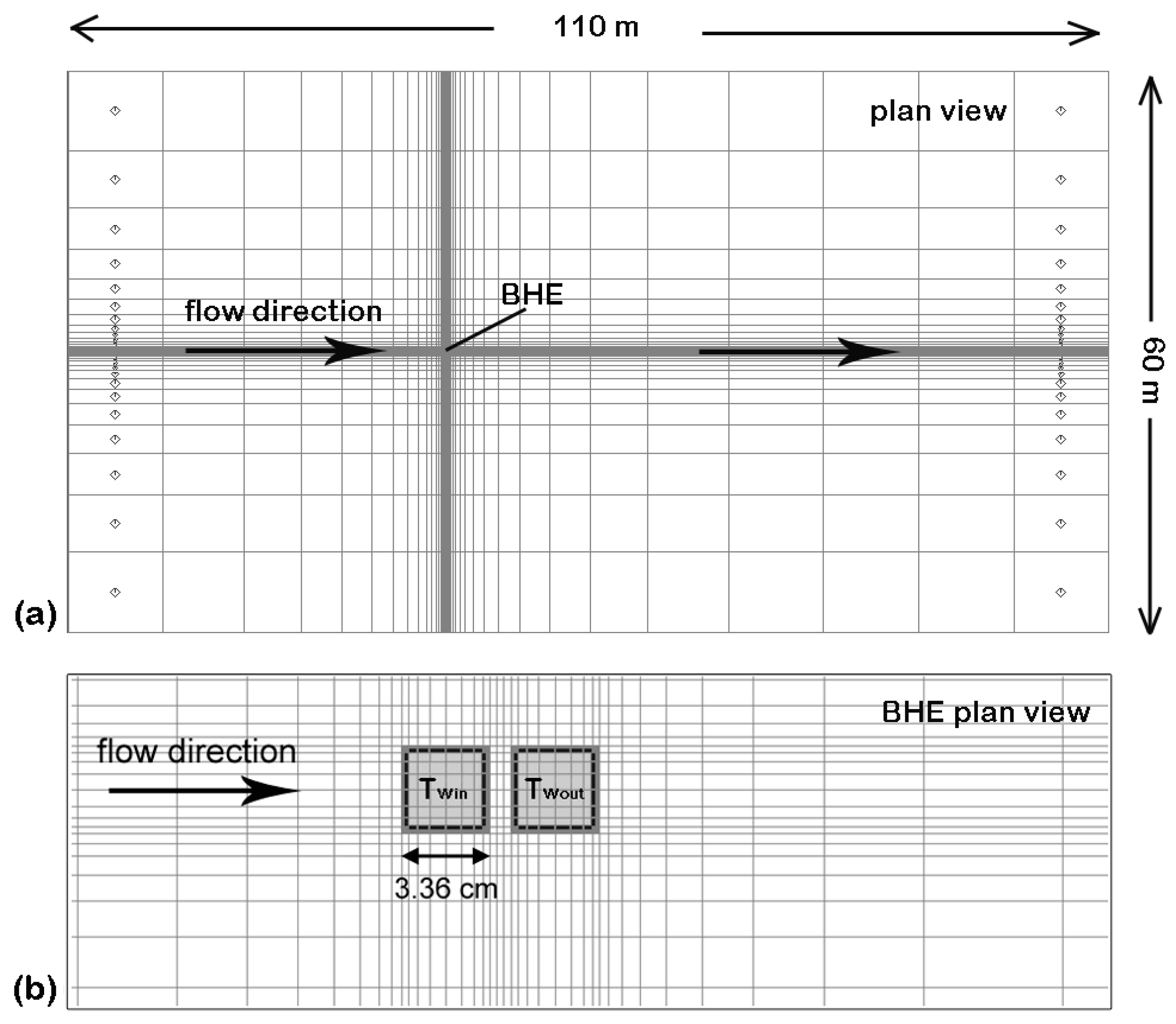
Figure 2.
Horizontal cross section of a typical BHE.
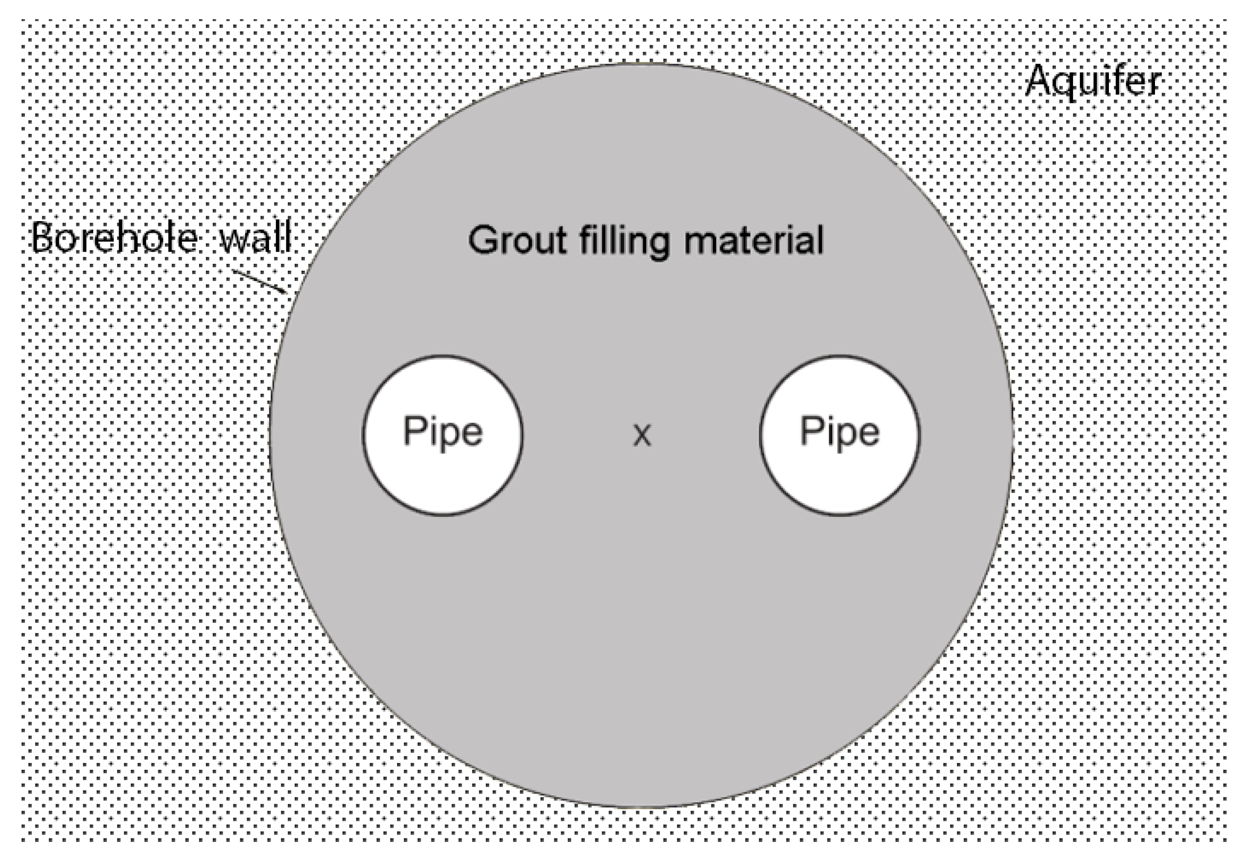
Figure 3.
Total seasonal energy extracted from the ground versus Darcy velocity, for different grouts.
Figure 3.
Total seasonal energy extracted from the ground versus Darcy velocity, for different grouts.

Figure 4.
Heat rate extracted from the ground versus time, for different Darcy velocities and different grouts.
Figure 4.
Heat rate extracted from the ground versus time, for different Darcy velocities and different grouts.
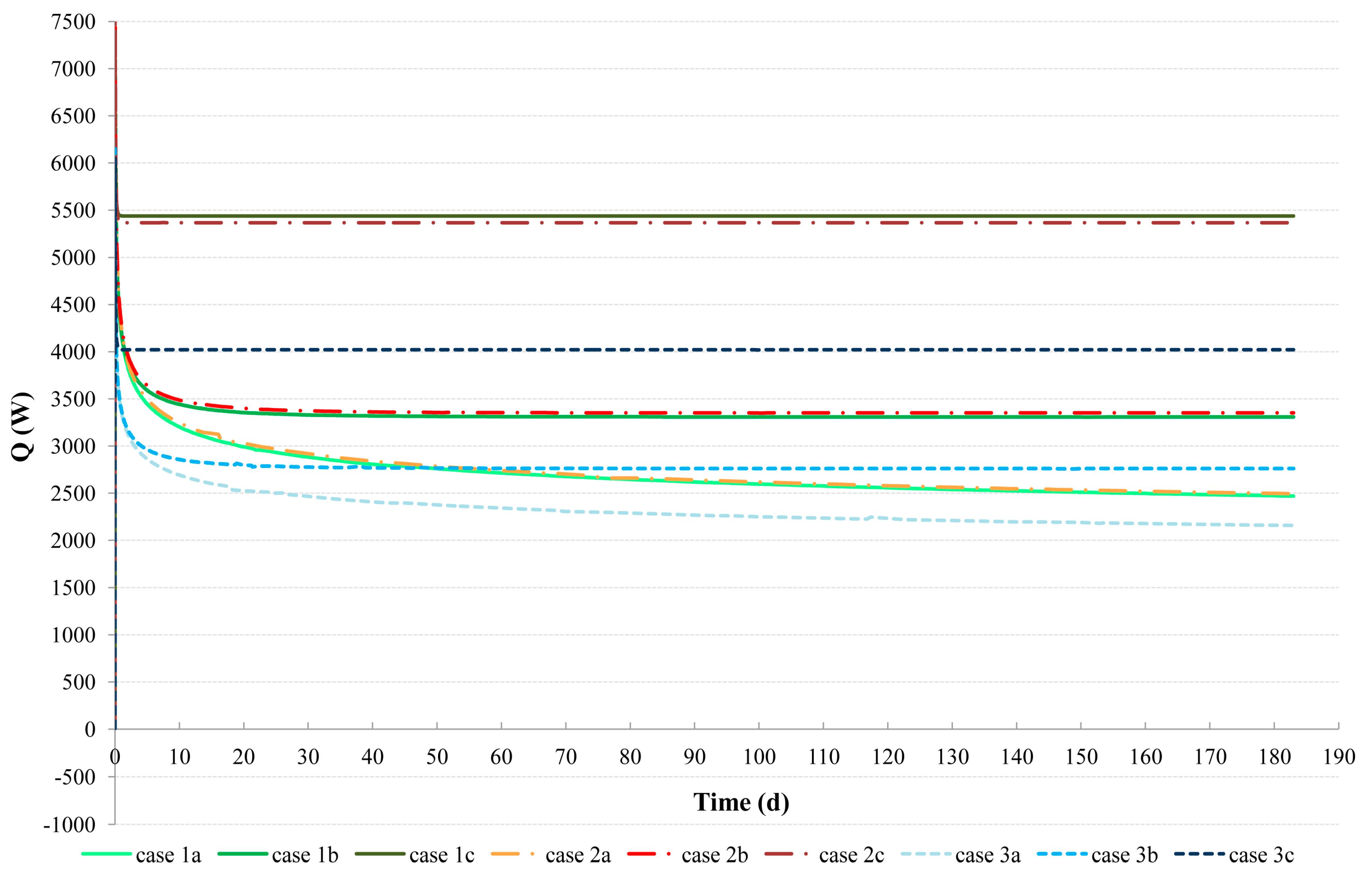
Figure 5.
Composition of the total thermal resistance in Case 1, Case 2 and Case 3 for different Darcy velocities and different borehole grouts.
Figure 5.
Composition of the total thermal resistance in Case 1, Case 2 and Case 3 for different Darcy velocities and different borehole grouts.

Figure 6.
Ground temperature versus distance from the BHE, for different Darcy velocities and different borehole grouts at t = 183 days (winter period end).
Figure 6.
Ground temperature versus distance from the BHE, for different Darcy velocities and different borehole grouts at t = 183 days (winter period end).

Figure 7.
Plan view of aquifer temperature perturbations for Darcy velocity equal to 10−5 m/s and different borehole grouts (Case 1c top; Case 2c middle; Case 3c bottom) at t = 183 days (winter period end); aquifer undisturbed temperature is 11.8 °C.
Figure 7.
Plan view of aquifer temperature perturbations for Darcy velocity equal to 10−5 m/s and different borehole grouts (Case 1c top; Case 2c middle; Case 3c bottom) at t = 183 days (winter period end); aquifer undisturbed temperature is 11.8 °C.


Table 1.
Porous medium thermal and hydrogeological properties.
| Porosity | θ | 0.35 |
|---|---|---|
| Dispersivity | d | 0 m |
| Effective thermal conductivity | λm | 2.3 W/(m·K) |
| Volumetric thermal capacity | Cm | 2.72 MJ/(m3·K) |
| Hydraulic conductivity | km | 2 × 10⁻⁴ m/s |
| Darcy velocities | vi | 0; 10−6; 10−5 m/s |
Table 2.
Thermal and hydrogeological properties of the pipe wall.
| Porosity | θp | 0.02 |
|---|---|---|
| Dispersivity | dp | 0 m |
| Thermal conductivity | λp | 0.38 W/(m·K) |
| Volumetric thermal capacity | Cp | 1.78 MJ/(m3·K) |
| Hydraulic conductivity | kp | 1 × 10⁻²¹ m/s |
Table 3.
Simulated cases: borehole back-filling properties and thermal resistance calculated with GLHEPRO tool (Rbh percentage differences are related to Case 1).
Table 3.
Simulated cases: borehole back-filling properties and thermal resistance calculated with GLHEPRO tool (Rbh percentage differences are related to Case 1).
| Simulated Cases | Darcy Velocity (m/s) | ||||||||
|---|---|---|---|---|---|---|---|---|---|
| Grout Type | Case | Back-Filling | λg (W·m−1 K−1) | kg (m/s) | θ | Rbh (m·K/W) | a | b | c |
| 1 | Ground | 2.3 | 2 × 10⁻⁴ | 0.35 | 0.0540 | 0 | 1 × 10⁻⁶ | 1 × 10⁻⁵ | |
| 2 | High thermal conductivity grout | 2.3 | 5 × 10⁻¹¹ | 0.2 | 0.0540 | 0 | 1 × 10⁻⁶ | 1 × 10⁻⁵ | |
| 3 | Low thermal conductivity grout | 0.7 | 5 × 10⁻¹¹ | 0.2 | 0.1354 (+151%) | 0 | 1 × 10⁻⁶ | 1 × 10⁻⁵ | |
Table 4.
Total seasonal energy exchanged by the BHE during the seasonal operation and the percentage differences related to Case 1.
Table 4.
Total seasonal energy exchanged by the BHE during the seasonal operation and the percentage differences related to Case 1.
| Total Seasonal Energy (kWh) | Percentage Differences (%) | ||||
|---|---|---|---|---|---|
| Case | 1 | 2 | 3 | Case 2 vs. 1 | Case 3 vs. 1 |
| a | 11,871.6 | 11,979.1 | 10,220.2 | 0.9 | −13.9 |
| b | 14,666.9 | 14,858.7 | 12,226.1 | 1.3 | −16.6 |
| c | 23,888.8 | 23,579.9 | 17,661.9 | −1.3 | −26.1 |
© 2017 by the authors. Licensee MDPI, Basel, Switzerland. This article is an open access article distributed under the terms and conditions of the Creative Commons Attribution (CC BY) license (http://creativecommons.org/licenses/by/4.0/).
Share and Cite
MDPI and ACS Style
Alberti, L.; Angelotti, A.; Antelmi, M.; La Licata, I. A Numerical Study on the Impact of Grouting Material on Borehole Heat Exchangers Performance in Aquifers. Energies 2017, 10, 703. https://doi.org/10.3390/en10050703
AMA Style
Alberti L, Angelotti A, Antelmi M, La Licata I. A Numerical Study on the Impact of Grouting Material on Borehole Heat Exchangers Performance in Aquifers. Energies. 2017; 10(5):703. https://doi.org/10.3390/en10050703
Chicago/Turabian StyleAlberti, Luca, Adriana Angelotti, Matteo Antelmi, and Ivana La Licata. 2017. "A Numerical Study on the Impact of Grouting Material on Borehole Heat Exchangers Performance in Aquifers" Energies 10, no. 5: 703. https://doi.org/10.3390/en10050703
Note that from the first issue of 2016, this journal uses article numbers instead of page numbers. See further details here.