
Modeling and Optimization of a CoolingTower-Assisted Heat Pump System


College of Civil Engineering, Hunan University, Changsha 410082, China
*
Authors to whom correspondence should be addressed.
Energies 2017, 10(5), 733; https://doi.org/10.3390/en10050733
Submission received: 15 April 2017
/
Revised: 16 May 2017
/
Accepted: 17 May 2017
/
Published: 20 May 2017
(This article belongs to the Special Issue Solar Energy Application in Buildings)
Abstract
:To minimize the total energy consumption of a cooling tower-assisted heat pump (CTAHP) system in cooling mode, a model-based control strategy with hybrid optimization algorithm for the system is presented in this paper. An existing experimental device, which mainly contains a closed wet cooling tower with counter flow construction, a condenser water loop and a water-to-water heat pump unit, is selected as the study object. Theoretical and empirical models of the related components and their interactions are developed. The four variables, viz. desired cooling load, ambient wet-bulb temperature, temperature and flow rate of chilled water at the inlet of evaporator, are set to independent variables. The system power consumption can be minimized by optimizing input powers of cooling tower fan, spray water pump, condenser water pump and compressor. The optimal input power of spray water pump is determined experimentally. Implemented on MATLAB, a hybrid optimization algorithm, which combines the Limited memory Broyden-Fletcher-Goldfarb-Shanno (L-BFGS) algorithm with the greedy diffusion search (GDS) algorithm, is incorporated to solve the minimization problem of energy consumption and predict the system’s optimal set-points under quasi-steady-state conditions. The integrated simulation tool is validated against experimental data. The results obtained demonstrate the proposed operation strategy is reliable, and can save energy by 20.8% as compared to an uncontrolled system under certain testing conditions.
1. Introduction
With rapid economic development and improvement of living standard, energy demand in buildings has increased in China. Central air conditioning systems have been widely used, and their energy consumptions account for over 40% of the total energy consumption in buildings [1]. In cooling load-dominated areas, the cooling tower-assisted heat pump (CTAHP) system is a suitable alternative as the cold and heat sources for central air conditioning systems with the same advantage as common water-cooling air conditioners and water source heat pumps. Obviously, the efficient operation of CTAHP systems exerts significant implication on the energy-saving of central air conditioning systems.
Numerous studies have highlighted the potential impact of optimization on energy consumption of cooling tower-assisted air conditioning systems. The significant energy saving potential of cooling tower-assisted chiller systems can be estimated by using different optimization strategies, such as an energy optimization methodology [2], multi-objective evolutionary algorithms [3], an effective and robust chiller sequence control strategy [4], a multivariable Newton-based extremum-seeking control (ESC) scheme [5], an optimal approach temperature (OAT) control strategy [6], a data-driven approach with a two-level intelligent algorithm [7], etc.
Apart from this effort, efficient operation of CTAHP systems can also be effectively achieved by using different optimal operation strategies, such as thermodynamic and thermoeconomic optimization with evolutionary algorithms [8], numerical simulation with TRNSYS [9], a golden section search algorithm [10], etc. In addition, some researchers have focused on the optimal control strategies to reduce the total power consumption of central air conditioning systems. For example, Ma and Wang [11] presented a model-based supervisory and optimal control strategy for a central chiller plant to enhance the system performance and energy efficiency with 0.73–2.25% of daily energy savings via a reference using traditional settings. All these studies above demonstrated the energy-saving potential of air conditioning systems associated with the application of different control techniques.
To minimize the total energy consumption of the CTAHP system in cooling mode, a model-based control strategy with hybrid optimization algorithm for the system is presented in this paper. An existing experimental CTAHP system, which has been designed, built and tested in Hunan University, China, is selected as the study object. The system was originally designed to provide hot water. In order to find out the effects of sprayed antifreeze on the system efficiency under frost prevention conditions, Cheng et al. [12] conducted a series of experiments and developed heat and mass transfer models of the cooling tower. They found that when ambient wet-bulb temperature is below 3.6 °C, spray antifreeze could improve the system efficiency by 5% to 11%. In this paper, theoretical and empirical formulas are adopted to model the nonlinear relationship among the operating variables of the system. Four variables, viz. the desired cooling load, the ambient wet-bulb temperature, the temperature and flow rate of chilled water at the inlet of the evaporator, are set as independent variables. The system energy consumption can be minimized by optimizing the input powers of the cooling tower fan, the spray water pump, the condenser water pump and compressor. The optimal input power of the spray water pump is determined experimentally. A hybrid algorithm [13] that combines the Limited memory Broyden-Fletcher-Goldfarb-Shanno (L-BFGS) algorithm [14] with the Greedy Diffusion Search (GDS) algorithm, is used to search for the optimal set points of the other three independent variables. The models, experimental data and the hybrid optimization algorithm are coded and implemented in the Matlab environment. The results demonstrate the proposed control strategy is reliable, and can offer a remarkable energy saving under certain testing conditions.
2. System Description
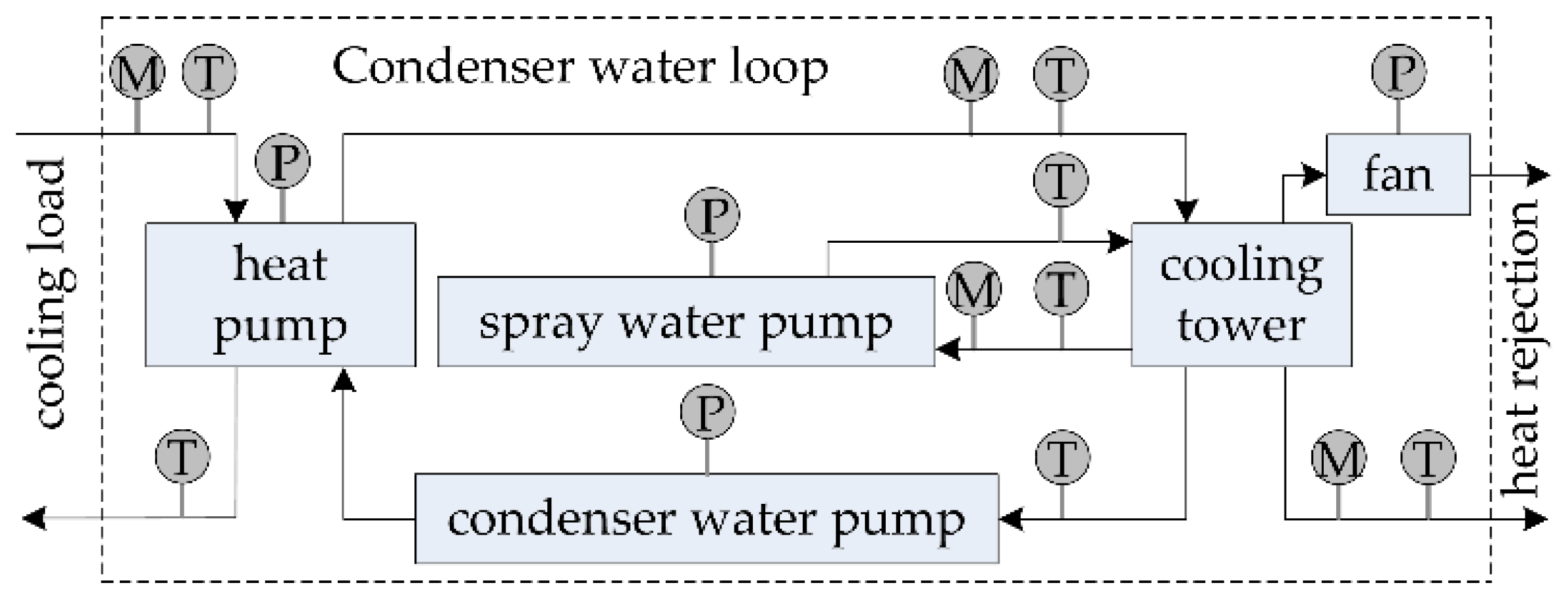
Figure 1 illustrates the schematic diagram of the CTAHP system in cooling mode. The system comprises a closed wet cooling tower (CWCT) with counter flow construction, a water source heat pump (WSHP) unit, a condenser water pump, a spray water pump, valves and connection tubes. The counter-flow CWCT is an important component of the CTAHP system. In the CWCT unit, there are three fluids, viz. spray water, condenser water and air. The air enters into the tower and goes through the finned heat-exchanger coil from bottom to top, while the condenser water and spray water flow through the coil from top to bottom, and the heat and mass transfer are completed in the course of flow. Another important part of the system is the WSHP unit which is coupled into the CWCT as a cooling source. The cooling water is fed by the circulating pump to the condenser of the WSHP unit, and then returns to the tower after being heated by the refrigerant of R22. Meanwhile, the chilled water is cooled by the refrigerant in the evaporator. In Figure 1, M, T and P indicate the mass flow rate, temperature and input power measurements, respectively.
3. Formulation of the Optimization Problem
3.1. Mathematical Modeling
Nonlinearity and complexity exist inherently in the dynamic process of the whole integrated CTAHP system, which makes it different to represent accurately using only theoretical approaches. Approaches combining theoretical and empirical methods are adopted herein to allow for performance prediction over a very wide range of operating conditions. Modeling approaches for most of the system components, including the heat pump, cooling tower, fan and pumps, as shown in Figure 1, are described as follows.
3.1.1. Heat Pump Model
The cooling load is expressed as follows:
During the cooling process, the heat pump is typically a vapor-compression refrigerant device. The power consumption of the water-to-water scroll heat pump is a function of the cooling load, the chilled water temperature at the inlet of the evaporate and the condenser water temperature at the inlet of the tower [15,16]. A regression function is used to describe the relationship of the power consumption and these variables, which is expressed as follows [17].
As the heat pump unit is treated as a single unit for modeling, the energy balance of the subsystem can be expressed as follows [18]:
3.1.2. Cooling Tower Model
A counter-flow heat exchanger with fins is used in the CWCT. The air inside the tower is sucked into the heat exchanger by means of an axial fan on the tower. The condenser water passing through the heat exchange coil heats the air outside the tubes. The heat transfer rate in the heat exchanger can be determined by the following relation:
3.1.3. Fan and Pump Models
3.1.4. Uncertainty Analysis
In Equations (1)–(8), there are seven input variables, viz. ambient wet-bulb temperature, inlet temperature and flow rate of the chilled water, and the power consumptions of the compressor, condenser water pump, spray water pump and cooling tower fan. The eight output variables include water temperatures at the inlet and outlet of the condenser, flow rates of condenser water and air, the cooling capacity of the heat pump unit and the heat rejection rate of the cooling tower unit, the dynamic viscosity coefficient of condenser water, and outlet chilled water temperature. The outcomes can be calculated by solving Equations (1)–(8) simultaneously.
In the present study, the coefficient of performance (COP) of the heat pump unit and the CTAHP system were chosen as performance indices, which were introduced as follows:
Uncertainty analyses for the experiment results could be calculated by the following equation [22]:
In order to compare the predicted performance indices and their deviation from the measured data, the mean squared error (MSE) is selected as the performance metric. The values of MSE average errors close to zero means a more useful prediction. Compared to mean bias error and mean absolute error, MSE is analytically tractable and measures the precision (variance) and accuracy (bias) [23], which is defined as follows: (y*: predicted value, y: measured value).
3.2. Objective Function and Inequality Constraints
In the CTAHP system, three types of devices, viz. compressor, fan and pumps, consume electric energy. The objective function, which is to minimize the systemic energy consumption when the required cooling load is satisfied, is expressed as follows:
The optimization problem is formulated through the determination of the controlled variables to achieve a minimum of an objective function subject to constraints. The objective is the power consumption of the CTAHP system. The decision variables are the power consumptions of cooling tower fan, condenser water pump, spray water pump and compressor. The uncontrollable variables include ambient wet-bulb temperature, inlet temperature and flow rate of the chilled water. Other dependent variables are the heat rejection rate of the cooling tower, the cooling capacity of the heat pump unit, the dynamic viscosity coefficient of water at the temperatures Tcw,i, the flow rate of air and condenser water. The mathematical formulations of the equality constraints are described as shown in Section 3.1, and the physical explanations of the inequality constraints are given below.
The input powers of the compressor, fan, condenser water pump and spray water pump are restricted by boundaries that are often provided by the manufacturers for the safe operation of the CTAHP system, which are expressed as follows:
Here, the data for a water-loop heat pump under cooling conditions are specified in one of China's national industry standards [24], as follows:
In the cooling tower, the ideal minimum temperature of the condenser water is the ambient wet bulb temperature, while the actual value is larger than the ideal value, which is expressed as:
The temperature difference between the inlet and outlet condenser water of tower is usually not greater than 5 °C, which can be expressed as [19]:
3.3. An Appropriate Optimization Algorithm and its Settings for the Problem at Hand
In order to better carry out the following analysis, fifteen operating variables of the CTAHP system are reclassified as follows. The four known variables include the ambient wet-bulb temperature, the desired cooling load, the flow rate and temperature of the chilled water at the inlet of the evaporator. The optimal input power of the spray water pump is determined experimentally. The other ten variables are listed in Table 1, and their symbols are unified for notational simplicity.
The constrained global optimization problem in Section 3.2, which is referred to as Problem (P), can be rewritten as follows:
Using the exact penalty function approach for nonlinear constrained optimization problems, the constraint functions can be augmented to the objective function, which is proposed in Reference [25]. The constraint violation function on X can be defined as follows:
For a given , the following penalty function on can be defined as follows:
Instead of solving Problem (P) directly, the following optimization problem should be considered:
For notational simplicity, z = (x, ϵ) and . Then, Problem (P) can be written as:
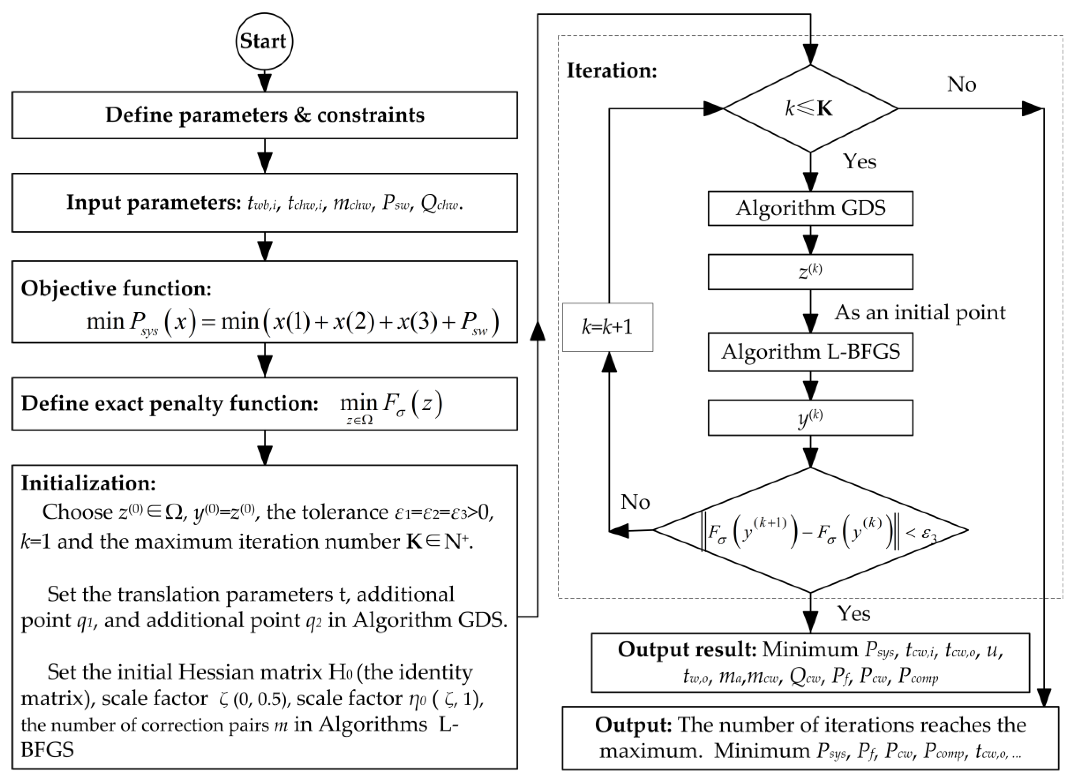
Algorithm limited memory BFGS (L-BFGS) is usually selected for the unconstrained optimization problem, and it has excellent performance for local search [26]. To enable the algorithm L-BFGS to escape from local minima, Liu et al. [13] proposed a hybrid approach which combined L-BFGS with a stochastic search strategy, namely the Greedy Diffusion Search (GDS). The results have shown that this method can achieve higher accuracy with a lower number of function evaluations. More details on the definition of Algorithm L-BFGS, Algorithm GDS and Algorithm hybridizing L-BFGS with GDS (L-GDS) can be found in Refs. [13,14]. Based on the hybridizing L-BFGS with GDS algorithms, the MATLAB optimization flowchart proposed in this paper, specifying inputs and outputs of the model, is illustrated in Figure 2.
4. Experiments
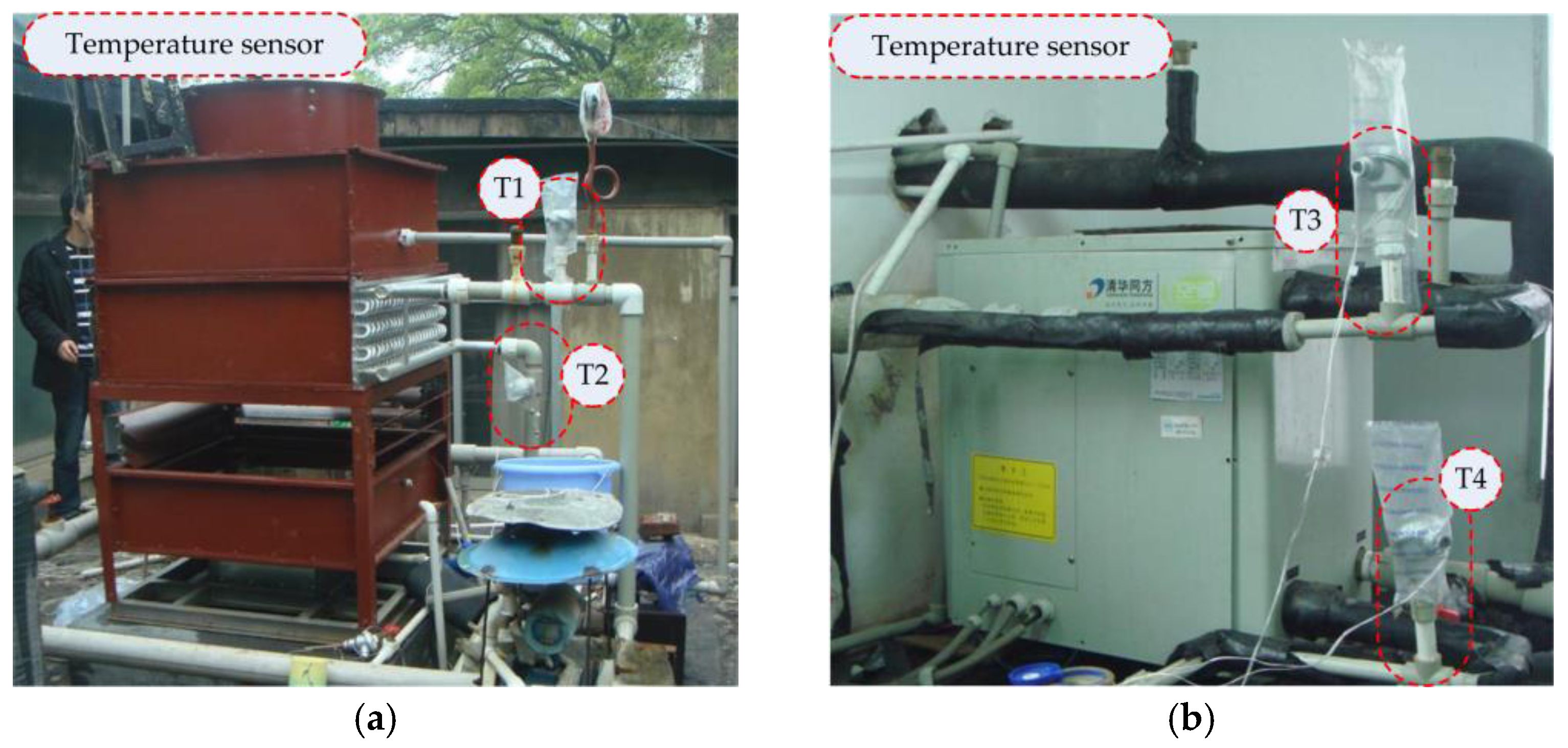
In this paper, an experimental CTAHP system has been selected for modeling as an example. The system, located on the rooftop of a single-story building at Hunan University of China, was originally designed as a heating source for hot water supply [12,27]. As shown in Figure 3a, the closed wet cooling tower was an induced draft counter-flow type and specially designed, and Figure 3b showed that the heat pump system was an integrated water-to-water HP unit with a rated power of 3.1 kW and a total cooling capacity of 15.3 kW. The rated powers of the fan and the condenser water pump were 0.55 kW and 0.75 kW, respectively. The rated power of the spray water pump was divided into three grades adjustable, viz. 0.200 kW, 0.175 kW and 0.150 kW. More details of the experimental set-up could be found in Reference [12].
A well-equipped instrumentation system was deployed to measure various properties of the cooling process, such as flow rate, power consumption and temperature. The water flow rates were measured by the ultrasonic flowmeters (PFSE) with an accuracy of 1%. In addition, the air flow rate was measured by standard nozzles (GB14294) with an accuracy of 1%. The input powers of the fan, compressor and condenser water pump were controlled by frequency conversion control cabinet, and the input power of the spray water pump could be adjusted manually. The operating loads of compressor, condenser water pump and fan, all of which were equipped with VSDs, could vary from 10% to 110% of their rated values. The actual power consumptions of these energy consuming devices were measured by digital clamp multimeters (UT202A UNI-T) with an accuracy of 1.5%. For the measurement of ambient wet-bulb temperature and water temperatures at different locations, platinum resistance thermometers (PT100) with an accuracy of 0.2 °C were used. In Figure 3, T1, T2, T3 and T4 indicate the condense water temperatures sensors at the inlet and outlet of cooling tower, inlet and outlet chilled water temperatures sensors, respectively. The various readings of instruments were monitored continuously and recorded with color paperless recorders (EN880) every five minutes. When the acquired temperatures from the color paperless recorders fluctuated within ±0.2 °C for longer than 15 min, each set of data was selected for further analyses.
5. Results and Discussion
5.1. Experimental Data and Model Validation
A number of tests were performed with the CTAHP system under approximately steady states. The energy consumption of spray water pump was investigated experimentally when the other variables were constant. The results showed that the power consumption of spray water pump did not have a considerable effect on the cooling capacity of the cooling tower unit when it was adjusted to 0.150 kW, 0.175 kW and 0.200 kW. The reason was that the spray water flow rate was influenced by the power consumption of spray water pump monotonically. Spray water pump power consumption of 0.150 kW could provide a large enough spray water flow to ensure the external surfaces of the heat exchanger in the tower was fully wetted by the spray water. When the spray water moistened all the surfaces, the effect of the variation of spray water flow rate on the thermal performance of the cooling tower unit could be neglected [19,28]. Thus, the power consumption of the spray pump was selected as 0.150 kW for the following analysis. As shown in Table 2, 26 sets of typical experiment data were selected for determining the corresponding coefficients of the models as well as validating against the proposed models, which were described in Section 3.1.
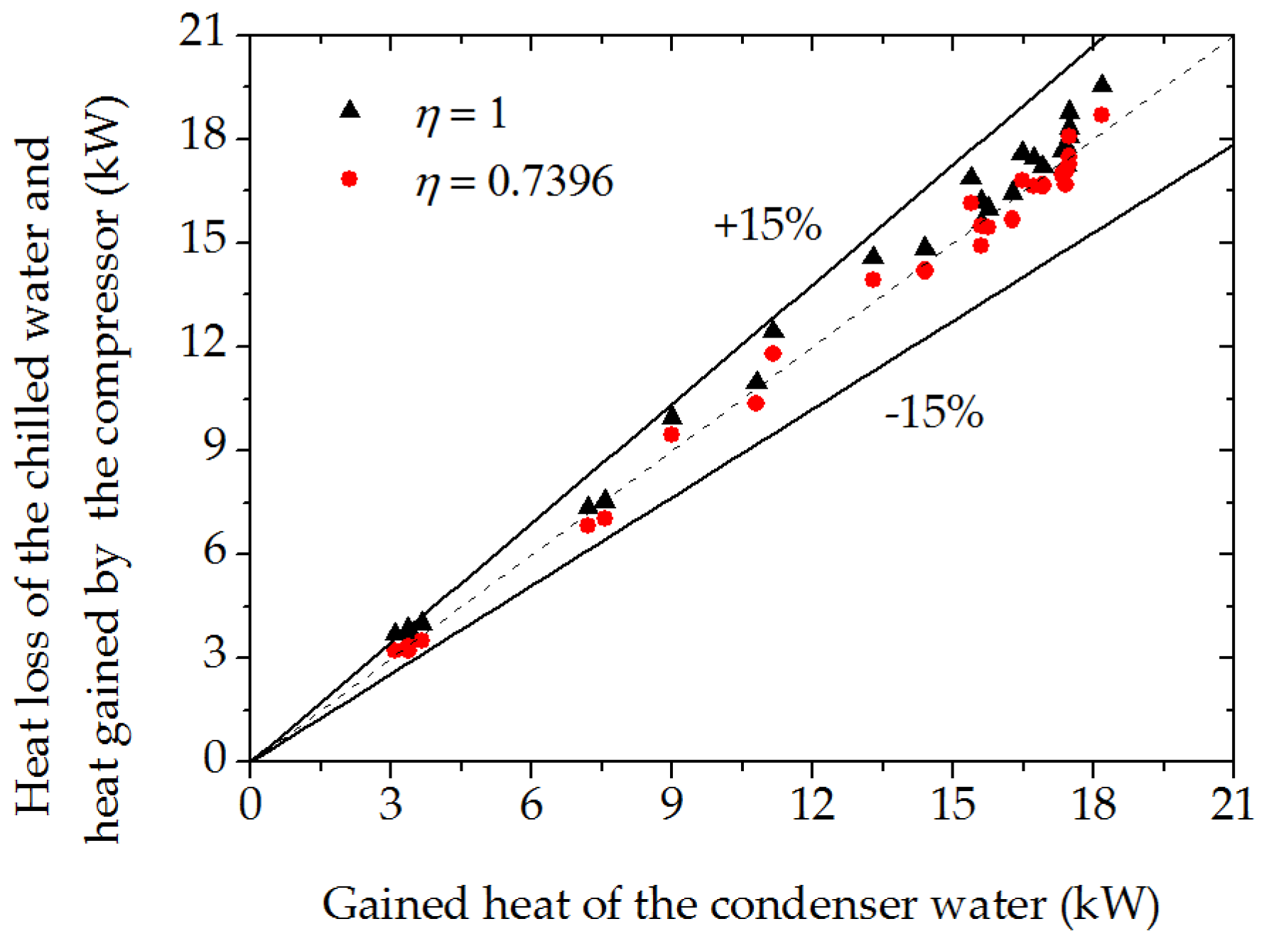
To verify the reliability of the experiment data, the energy balance of the heat pump unit was adopted. Based on the data provided by the manufacturer, the efficiencies of compressor and motor were both 86%. Therefore, η in Equation (5) was equal to 0.7396, viz. 0.86 multiplied by 0.86. At the same time, η = 1 in Ref. [18] was also selected for analyzing the energy balance. As shown in Figure 4, the unbalanced ratios of the heat gained by the condenser water and the heat lost by the chilled water and heat generated by the compressor were within ±15%. When η = 1 and η = 0.7396, the average absolute unbalanced ratios were 5.3% and 3.2%, respectively, which meant the data were reliable.
Based on well-established experimental data under quasi-steady-state conditions, when the least-square method and the confidence level of 95% were used, the regression results of the coefficients of Equations (2), (5), (7) and (8) were obtained, as listed in Table 3.
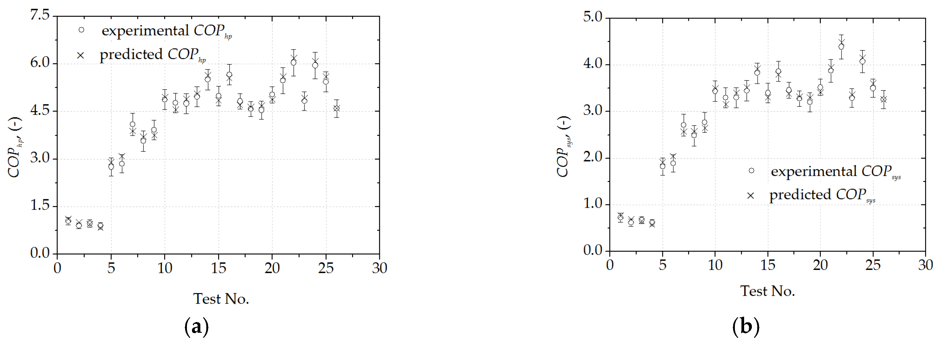
Figure 5 illustrates the predicted COPs, experimental COPs and their uncertainties. Model validation was carried out for predicting the COPhp, and COPsys. When the predicted values were compared with the measurements for the CTAHP system, the MSEs of COPhp, and COPsys were 0.0179 and 0.0081, respectively. Validation results indicated that the predicted COPs of the heat pump unit and the system were in good agreement with the experimental data, which meant the models were accuracy enough for performance prediction and further analysis of the CTAHP system. The uncertainty of COPhp, calculated based on the experimental data, was (8.1 ± 3.7)%. The uncertainty of COPsys was (9.0 ± 3.9)%, of which the uncertainty caused by the temperature difference between inlet and outlet chilled water accounted for (69.2 ± 0.9)% of the total uncertainty; while the uncertainties caused by the power consumptions of the system and the chilled water mass flow rate were (20.7 ± 6.4)% and (13.8 ± 4.5)%, respectively. Therefore, improving the temperature measurement accuracy can effectively improve the test accuracy.
5.2. Sensitivity Analysis
A sensitivity analysis was conducted to investigate the influences of the variation of six independent variables, viz. ambient wet-bulb temperature, inlet temperature and flow rate of chilled water, the input powers of compressor, fan and condenser water pump, on the COPs of the heat pump unit and the CTAHP system. Normal probability analyses of these independent variables were conducted with 26 sets of typical experiment data, as shown in Figure 6.
As listed in Table 4, the linear regression relations between COPs and these independent variables could be determined by curve fitting of experimental data with the least-square method and a confidence level of 95%. The sensitivity analysis was carried out using a sensitivity tool, Oracle’s Crystal Ball, which was the leading spreadsheet-based application for forecasting. The assumption, decision and forecast of the tool for the CTAHP system are given in Table 4. Figure 7 illustrates the sensitivity analysis results. Chilled water flow rate had a significant positive effect on the values of COPhp and COPsys, followed by fan input power. Compressor input power had a significant negative effect on the COPhp, while it had little effect on the COPsys. The effect of the other three variables on the COPhp is similar to that of the COPsys.
5.3. Energy Analysis
The mathematical model and experimental data for the system components were implemented in MATLAB. The codes were written with double precision arithmetic. For all the optimization problems below, the maximum number of iterations K = 5000. The translation parameter t = 1/3, additional points q1 = 10, additional points q2 = 5 in Algorithm GDS. The initial symmetric positive definite matrix H0 = I (the identity matrix), scale factor ζ = 0.25, scale factor η0 = 0.75, tolerance ε1 = ε2 = ε3 = 10−6 and the number of correction pairs m = 5 in Algorithm L-BFGS. During the execution of Algorithm L-BFGS, the numerical gradients were calculated by a two-point computational formula.
The optimal set-points, obtained from the proposed algorithm, were aimed at minimizing systemic power consumption while fulfilling the cooling load. The operating loads of the compressor, condenser water pump, and fan, all of which were equipped with VSDs, could vary from 10% to 110% of their rated values. The specifications of the system and operating conditions for the considered case are given in Table 5.
5.3.1. Effect of the Two Controlled Variables at a Required Cooling Load
As depicted in Figure 8a,b, any addition to the compressor power consumption would lead to decrease the power consumption of condenser water pump or fan power consumption. Further increasing the compressor power consumption could significantly increase the system power consumption, which meant the compressor power consumption had a high impact on the system power consumption. This was because the compressor power consumption directly affected the refrigerant flow rate and the temperature difference of the refrigerant in the condenser and evaporator. The flow rate and temperature of the refrigerant in the evaporator determined the ability of the heat pump unit to absorb heat from the chilled water, while those in the condenser affected the heat rejection rate of the unit. Figure 8c illustrates that the trend of fan power consumption was opposite to that of the power consumption of condenser water pump. This meant the condenser water flow rate was increased with the decrease of the air flow rate when the heat rejection rate of the cooling tower was constant, which was consistent with the results of our previous study [18]. In addition, the system power consumption was slightly decreased with the decrease of the pump power consumption and the increase of the fan power consumption, which meant the impact of the power consumption of condenser water pump on the system power consumption was greater than that of cooling tower fan.
5.3.2. Effect of Three Controlled Variables at a Desired Cooling Load
As shown in Figure 9a, the variations of the power consumptions of the compressor, condenser water pump and cooling tower fan were investigated for the case study. The results showed that the compressor power consumption should be lowered in the process of system optimization operation. Figure 9b,c shows that the system power consumption changed with the controlled variables three-dimensionally and two-dimensionally, respectively. At this optimal set-point, the fan power consumption was very close to its maximum, 0.605 kW. The power consumption of the condenser water pump was slightly higher than its rated value, 0.750 kW, and the compressor power consumption was approximately two thirds of its rating. These results suggest that for a required cooling load, moderate increase in fan energy consumption is conducive to reducing system energy consumption, while excessive compressor energy consumption is not conducive to system energy saving.
5.3.3. Effect of the Three Controlled Variables at Different Required Cooling Loads
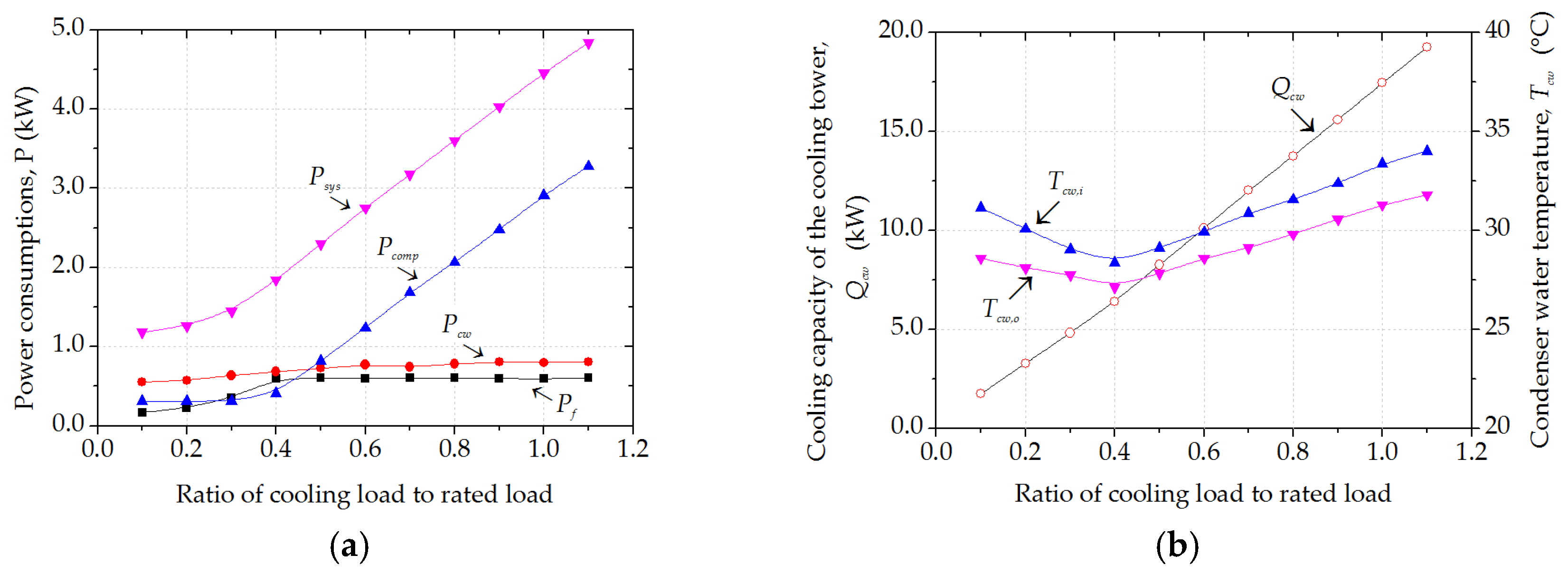
As the ratio of cooling load to rated load increased, the optimal power consumptions of the CTAHP system and its components were investigated, as shown in Figure 10a. When the ratio of cooling load to rated load was below 0.4, the growth of system power consumption was mainly caused by the increase in fan power consumption. And the ratio of cooling load to rated load varied from 0.4 to 1.1, the increase of the compressor power consumption directly caused a significant increase in the system power consumption. Moreover, Figure 10a illustrates the power consumption of the condenser water pump increased gradually with the increase of the ratio. Figure 10b shows that the cooling capacity of the cooling tower increased with the increase in the ratio of cooling load to rated load, and the condenser water temperatures at the inlet and outlet were lowest at the ratio of 0.4.
5.4. Analysis of Energy Saving Potential under Test Operating Conditions
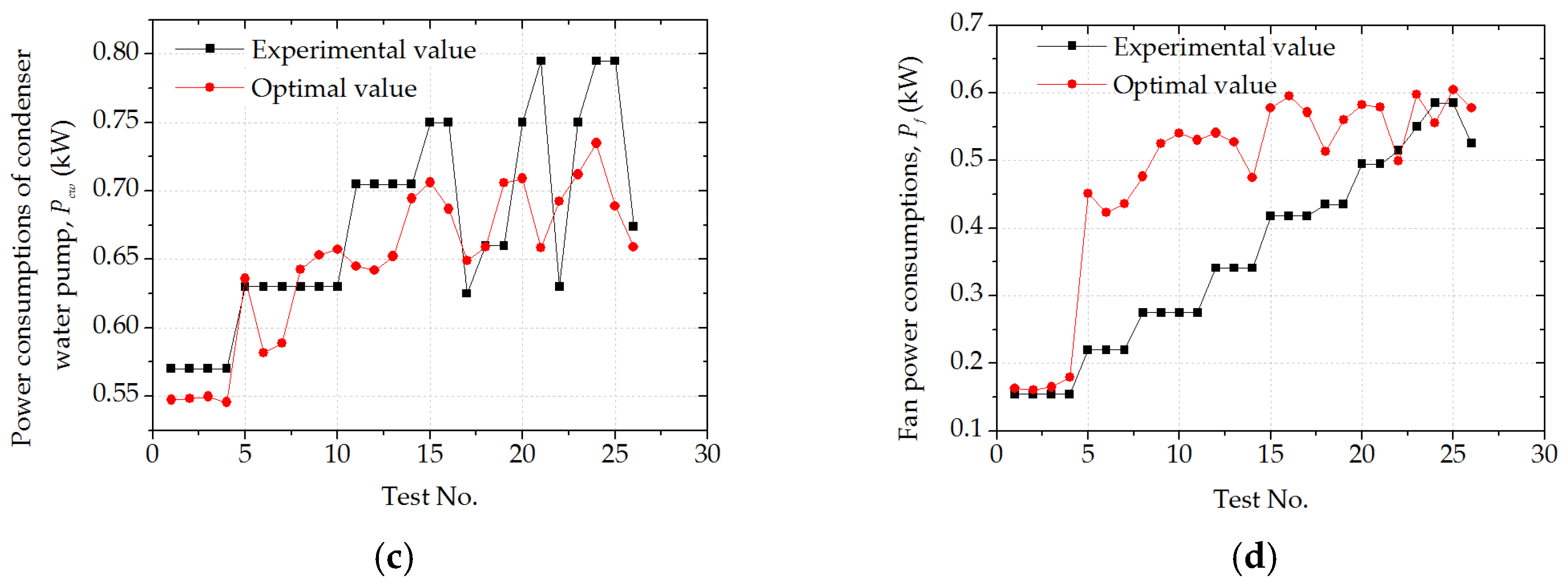
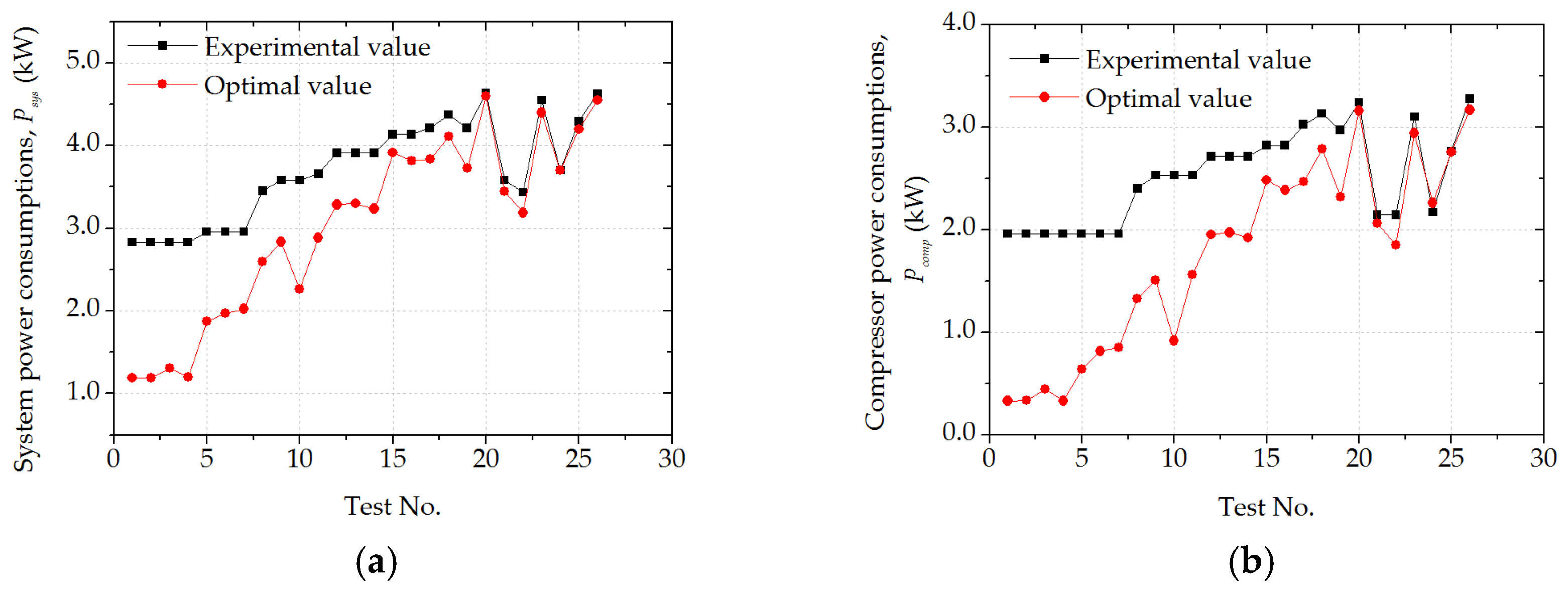
The required cooling load, measured uncontrollable variables, and other initial values obtained from the proposed L-GDS algorithm were fed to MATLAB in order to compute the optimal set-points of the controlled variables. These optimal set-points were aimed to minimize the systemic power consumption while fulfilling the desired cooling load. As shown in Figure 11a–d, the power consumptions of the system and its components without optimization were compared to those with optimization. The results showed that the average systemic power consumption with optimization was nearly 20.8% less than that without optimization. Power consumption values of the compressor and condenser water pump with optimization were generally less than those without optimization while the fan power consumption was higher than that without optimization. The energy savings potential for the compressor and condenser water pump were 34.1% and 3.5%, respectively, while the cooling tower fan power consumption increased by 40.3%. The reason was that a higher fan power consumption caused a lower condenser water temperature and required a lower refrigerant superheat temperature entering the condenser. When the power consumption of condenser water pump slightly decreased as a result of the increased fan power consumption, the compressor power consumption also reduced because a lower condensing pressure was required. Meanwhile, as the fan power consumption increased, the system power consumption became lower. Therefore, an appropriate increase in the fan power consumption was conducive to significantly reduce the power consumptions of the CTAHP system and compressor. In addition, the results obtained showed a relatively high influence of the compressor power consumption on the system power consumption. From this discussion, the proposed optimal control strategy could effectively ensure that the CTAHP system was guaranteed to meet the required cooling load while the system was working in good conditions.
6. Conclusions
In order to minimize the power consumption of a cooling tower-assisted heat pump (CTAHP) system under cooling conditions, the modeling and optimization problem of the system has been addressed, and the proposed approach has been verified on an experimental platform. An existing CTAHP system has been used for experimentation and data collection. By using the experimental data, the mathematical models for the systemic components have been developed and implemented in MATLAB to predict the system’s performance operating under various conditions. A novel hybrid optimization-simulation algorithm has been adopted to find the optimizing set-points of the power consumptions of the compressor, condenser water pump and cooling tower fan. The main conclusions are summarized below:
- (1)
- The predicted coefficient of performances (COPs) of the heat pump unit and the system are in good agreement with the experimental data, which means the modeling method is reliable and accurate for performance prediction of the CTAHP system.
- (2)
- Sensitivity analysis results demonstrate that chilled water flow rate has a significant positive effect on the values of COPhp and COPsys, followed by fan input power. Compressor input power has a significant negative effect on the COPhp, while it has little effect on the COPsys.
- (3)
- The average systemic power consumption with optimization is nearly 20.8% less than that without optimization under certain testing conditions.
The proposed operation strategy proposed in this paper is reliable, and it can significantly reduce the energy consumption of the CTAHP system in cooling mode, especially in part-load conditions.
Acknowledgments
The study has been supported by the China National Key R&D Program “Solutions to heating and cooling of buildings in the Yangtze River region” (Grant No. 2016YFC0700305). The authors also appreciated the financial support from National Natural Science Foundation of China (No. 51578220).
Author Contributions
Jianlin Cheng designed and built the CTAHP system. The measurement data was collected and analyzed by Xiaoqing Wei, Jianlin Cheng, Jinhua Hu, and Meng Wang. Xiaoqing Wei conducted the simulations, and accomplished the writing of the paper in close and steady cooperation with all authors. Nianping Li and Jinqing Peng guided the whole work and edited language.
Conflicts of Interest
The authors declare no conflict of interest.
Nomenclature
| m | mass flow rate, kg/s |
| T | temperature, °C |
| cw | specific heat of cooling water at constant pressure, 4.1868 kJ/(kg·°C) |
| cpsat | the fictitious specific heat of saturated air at constant pressure, kJ/(kg·°C) |
| H | Hessian matrix |
| P | power consumption, kW |
| Q | heat rejection rate, kW |
| x | x = (x(1), x(2), …, x(10))∈R10 |
| hi | continuously differentiable functions, Equation (i), i = 1, 2, …, 8 |
| gj | continuously differentiable functions, Equation (j), j = 16, 17 |
| L,U | L = [L1, L2, …, L10] and U = [U1, U2, …, U10] are, respectively, the lower and upper bounds of the ten unknown variables. |
| Greek Symbols | |
| μcw | dynamic viscosity coefficient of water at the temperatures Tcw,i, kg/(m·s) |
| μo | dynamic viscosity coefficient of water at 0 °C, 1.792 × 10⁻³ kg/(m·s) |
| α, β | positive constants, 1 ≤ β ≤ α |
| σ | penalty parameter, σ > 0 |
| βint | a constant which is influenced by the coil’s geometry and constant water-properties |
| βext | a constant which depends on the thermal properties of air and on the coil’s geometry |
| η | heat generated efficiency by the compressor |
| ζ, ηo | scale factor, 0 < ζ < 0.5, ζ < ηo < 1 |
| Subscripts | |
| a | air |
| f | cooling tower fan |
| sw | spray water |
| cw | condenser water |
| chw | chilled water |
| comp | compressor |
| i | inlet |
| o | outlet |
| wb | ambient wet-bulb |
References
- American Society of Heating, Refrigerating, and Air-Conditioning Engineers (ASHRAE). ASHRAE Handbook—2011 HVAC Applications; ASHRAE: Atlanta, GA, USA, 2011. [Google Scholar]
- Thangavelu, S.R.; Myat, A.; Khambadkone, A. Energy optimization methodology of multi-chiller plant in commercial buildings. Energy 2017, 123, 64–76. [Google Scholar] [CrossRef]
- Sayyaadi, H.; Nejatolahi, M. Multi-objective optimization of a cooling tower assisted vapor compression refrigeration system. Int. J. Refrig. 2011, 34, 243–256. [Google Scholar] [CrossRef]
- Shan, K.; Wang, S.; Gao, D.C.; Xiao, F. Development and validation of an effective and robust chiller sequence control strategy using data-driven models. Autom. Constr. 2016, 65, 78–85. [Google Scholar] [CrossRef]
- Mu, B.; Li, Y.; Seem, J.E.; Hu, B. A multivariable newton-based extremum seeking control for condenser water loop optimization of chilled-water plant. J. Dyn. Syst. 2015, 137, 111011. [Google Scholar] [CrossRef]
- Liu, C.W.; Chuah, Y.K. A study on an optimal approach temperature control strategy of condensing water temperature for energy saving. Int. J. Refrig. 2011, 34, 816–823. [Google Scholar] [CrossRef]
- Wei, X.; Xu, G.; Kusiak, A. Modeling and optimization of a chiller plant. Energy 2014, 73, 898–907. [Google Scholar] [CrossRef]
- Sayyadi, H.; Nejatolahi, M. Thermodynamic and thermoeconomic optimization of a cooling tower-assisted ground source heat pump. Geothermics 2011, 40, 221–232. [Google Scholar] [CrossRef]
- Chargui, R.; Sammouda, H.; Farhat, A. Numerical simulation of a cooling tower coupled with heat pump system associated with single house using TRNSYS. Energy Convers. Manag. 2013, 75, 105–117. [Google Scholar] [CrossRef]
- Yuan, S.; Grabon, M. Optimizing energy consumption of a water-loop variable-speed heat pump system. Appl. Therm. Eng. 2011, 31, 894–901. [Google Scholar] [CrossRef]
- Ma, Z.; Wang, S. Supervisory and optimal control of central chiller plants using simplified adaptive models and genetic algorithm. Appl. Energy 2011, 88, 198–211. [Google Scholar] [CrossRef]
- Cheng, J.; Li, N.; Wang, K. Study of heat-source-tower heat pump system efficiency. Procedia Eng. 2015, 121, 915–921. [Google Scholar] [CrossRef]
- Liu, J.; Zhang, S.; Wu, C.; Liang, J.; Wang, X.; Teo, K.L. A hybrid approach to constrained global optimization. Appl. Soft Comput. 2016, 47, 281–294. [Google Scholar] [CrossRef]
- Liu, D.C.; Nocedal, J. On the limited memory BFGS method for large scale optimization. Math. Program. 1989, 45, 503–528. [Google Scholar] [CrossRef]
- Braun, J.E.; Comstock, M.C. Development of Analysis Tools for the Evaluation of Fault Detection and Diagnostics for Chillers; Deliverable for Ashrae Research Project: Atlanta, GA, USA, 1999. [Google Scholar]
- Cheung, H.; Braun, J.E. Empirical modeling of the impacts of faults on water-cooled chiller power consumption for use in building simulation programs. Appl. Therm. Eng. 2016, 99, 756–764. [Google Scholar] [CrossRef]
- American Society of Heating, Refrigerating, and Air-Conditioning Engineers (ASHRAE). ASHRAE Handbook—1999 HVAC Applications Handbook; ASHRAE: Atlanta, GA, USA, 1999; Volume 40, pp. 1–36. [Google Scholar]
- Lu, L.; Cai, W.; Soh, Y.C.; Xie, L.; Li, S. HVAC system optimization—Condenser water loop. Energy Convers. Manag. 2004, 45, 613–630. [Google Scholar] [CrossRef]
- Wei, X.; Li, N.; Peng, J.; Cheng, J.; Hu, J.; Wang, M.; Sciubba, E. Performance analyses of counter-flow closed wet cooling towers based on a simplified calculation method. Energies 2017, 10, 282. [Google Scholar] [CrossRef]
- Stabat, P.; Marchio, D. Simplified model for indirect-contact evaporative cooling-tower behaviour. Appl. Energy 2004, 78, 433–451. [Google Scholar] [CrossRef]
- Kreider, J.F.; Curtiss, P.; Rabl, A. Heating and Cooling of Buildings: Design for Efficiency, 2nd ed.; CRC Press: Boca Raton, FL, USA, 2010. [Google Scholar]
- Kline, S.J.; Mcclintock, F.A. Describing uncertainties in single sample experiments. Mech. Eng. 1953, 78, 3–8. [Google Scholar]
- Afram, A.; Janabi-Sharifi, F. Review of modeling methods for HVAC systems. Appl. Therm. Eng. 2014, 67, 507–519. [Google Scholar] [CrossRef]
- General Administration of Quality Supervision, Inspection and Quarantine of the People’s Republic of China. GB/T 19409–2013 Water-Source (Ground-Source) Heat Pump; Standards Press of China: Beijing, China, 2013.
- Lin, Q.; Loxton, R.; Teo, K.L.; Wu, Y.H.; Yu, C. A new exact penalty method for semi-infinite programming problems. J. Comput. Appl. Math. 2014, 261, 271–286. [Google Scholar] [CrossRef]
- Xiao, Y.; Wei, Z.; Wang, Z. A limited memory BFGS-type method for large-scale unconstrained optimization. Comput. Math. Appl. 2008, 56, 1001–1009. [Google Scholar] [CrossRef]
- Wei, X.; Li, N.; Peng, J.; Cheng, J.; Su, L. Analysis of the effect of the CaCl2 mass fraction on the efficiency of a heat pump integrated heat-source tower using an artificial neural network model. Sustainability 2016, 8, 410. [Google Scholar] [CrossRef]
- Yoo, S.Y.; Kim, J.H.; Han, K.H. Thermal performance analysis of heat exchanger for closed wet cooling tower using heat and mass transfer analogy. J. Mech. Sci. Technol. 2010, 24, 893–898. [Google Scholar] [CrossRef]
Figure 1.
Schematic diagram of the CTAHP system under cooling conditions. M, T and P indicate the mass flow rate, temperature and input power measurements, respectively.
Figure 1.
Schematic diagram of the CTAHP system under cooling conditions. M, T and P indicate the mass flow rate, temperature and input power measurements, respectively.

Figure 2.
Flowchart of the optimization approach based on hybridizing L-BFGS with GDS algorithms.

Figure 3.
Photographs of: (a) closed wet cooling tower; and (b) water source heat pump unit. T1, T2, T3 and T4 indicate the condense water temperatures sensors at the inlet and outlet of cooling tower, inlet and outlet chilled water temperatures sensors, respectively.
Figure 3.
Photographs of: (a) closed wet cooling tower; and (b) water source heat pump unit. T1, T2, T3 and T4 indicate the condense water temperatures sensors at the inlet and outlet of cooling tower, inlet and outlet chilled water temperatures sensors, respectively.

Figure 4.
Energy balance of the HP unit test.

Figure 5.
The predicted COPs, experimental COPs and their uncertainties: (a) COPhp, (b) COPsys.

Figure 6.
Normal probability plots of: (a) ambient wet-bulb temperature; (b) chilled water inlet temperature; (c) chilled water flow rate; (d) fan input power; (e) input power of condenser water pump and (f) compressor input power.
Figure 6.
Normal probability plots of: (a) ambient wet-bulb temperature; (b) chilled water inlet temperature; (c) chilled water flow rate; (d) fan input power; (e) input power of condenser water pump and (f) compressor input power.
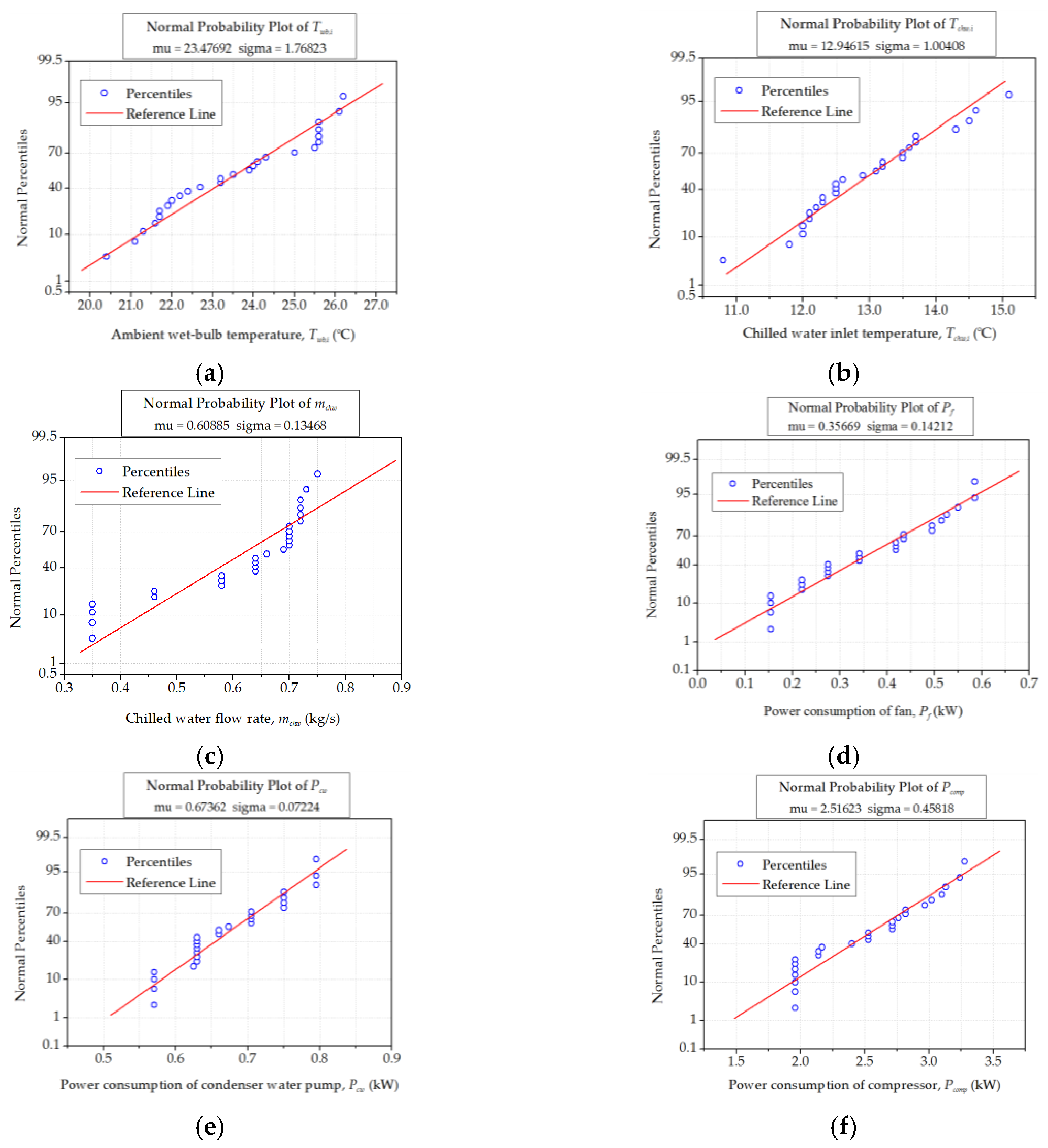
Figure 7.
Sensitivity analysis on the values of (a) COPhp and (b) COPsys.
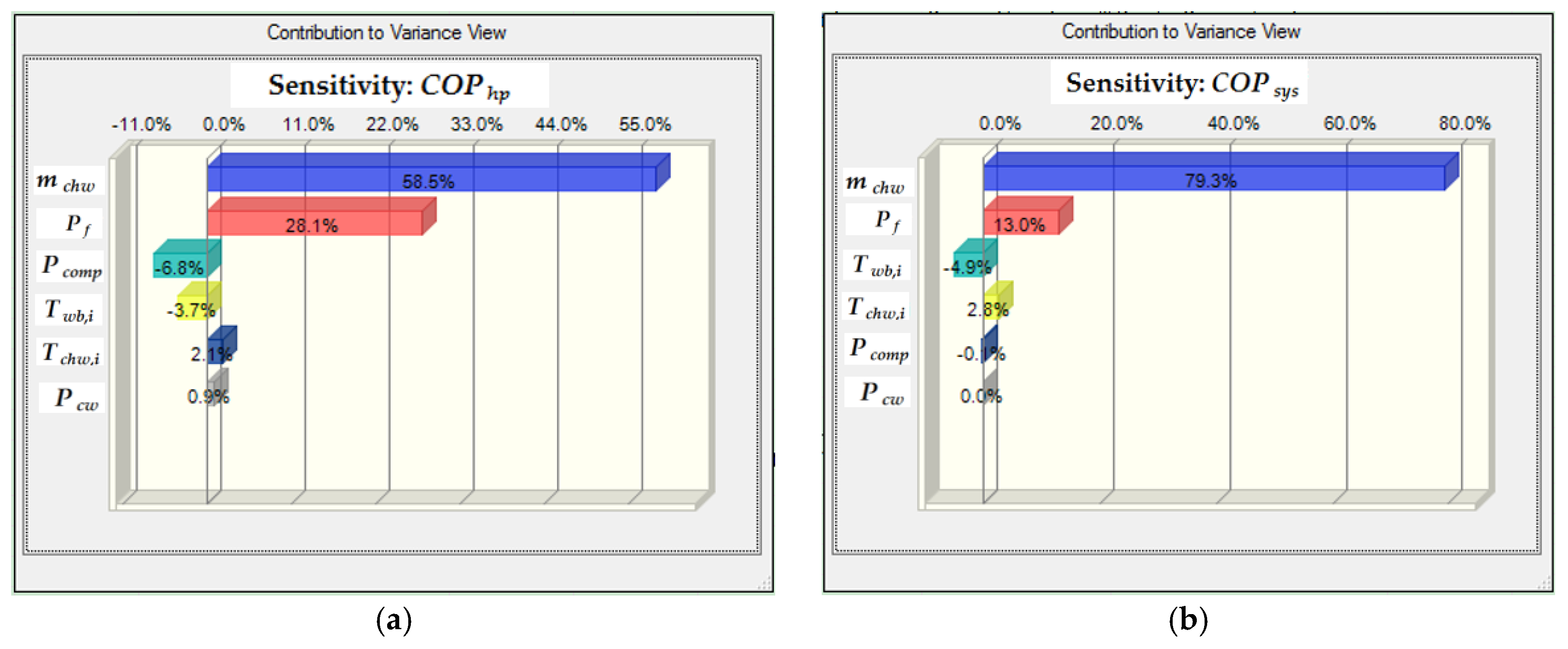
Figure 8.
Two optimal controlled variables at a required cooling load of 12.24 kW: (a) compressor input power versus the input power of condenser water pump; (b) compressor input power versus fan input power; (c) fan input power versus the input power of condenser water pump.
Figure 8.
Two optimal controlled variables at a required cooling load of 12.24 kW: (a) compressor input power versus the input power of condenser water pump; (b) compressor input power versus fan input power; (c) fan input power versus the input power of condenser water pump.
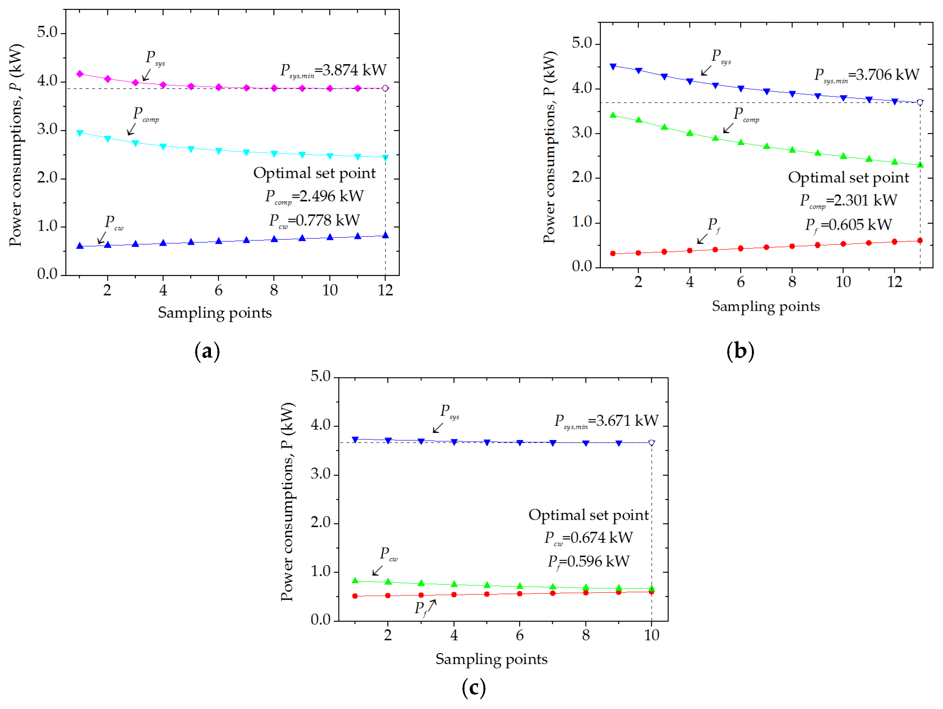
Figure 9.
Three optimally controlled variables at a required cooling load of 12.24 kW: (a) compressor power consumption versus the power consumptions of fan and condenser water pump; (b) system power consumption versus the power consumptions of fan and condenser water pump (Three-dimensional); and (c) system power consumption versus the power consumptions of fan and condenser water pump (Two-dimensional).
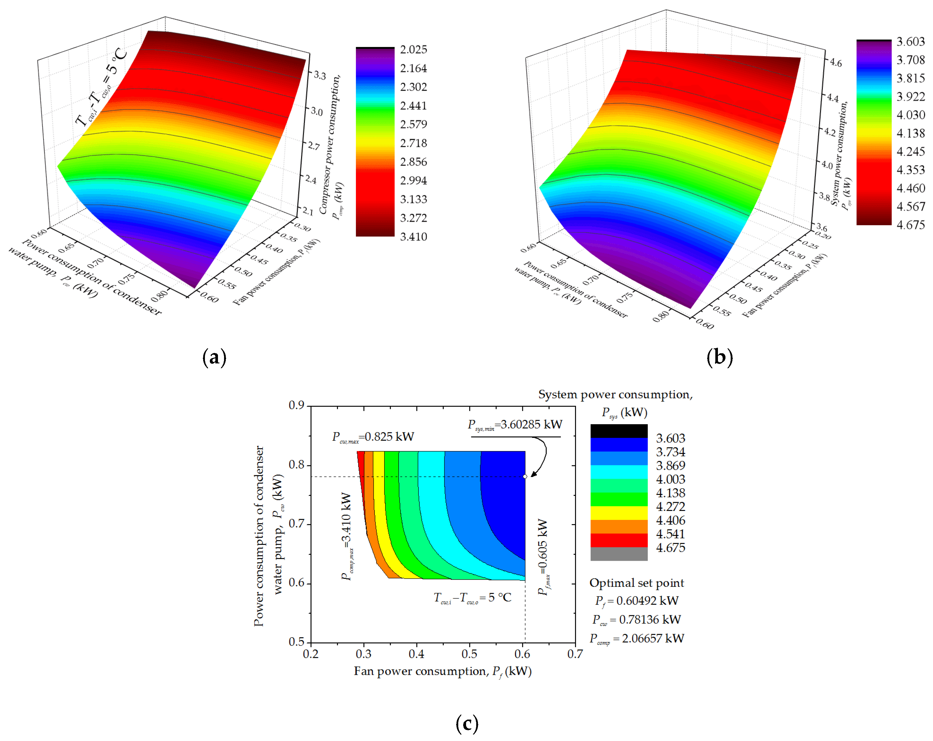
Figure 10.
Optimal variables at different ratios of cooling load to rated load: (a) minimum power consumptions of the CTAHP system and its optimal controlled variables; (b) cooling capacity and condenser water temperatures at the inlet and outlet of the cooling tower.
Figure 10.
Optimal variables at different ratios of cooling load to rated load: (a) minimum power consumptions of the CTAHP system and its optimal controlled variables; (b) cooling capacity and condenser water temperatures at the inlet and outlet of the cooling tower.

Figure 11.
Power consumptions of the devices: (a) system; (b) compressor; (c) condenser water pump; and (d) cooling tower fan.
Figure 11.
Power consumptions of the devices: (a) system; (b) compressor; (c) condenser water pump; and (d) cooling tower fan.


Table 1.
Ten unknown variables and their uniform symbols.
| Variables | Uniform Symbols | Variables | Uniform Symbols |
|---|---|---|---|
| Pf, kW | x(1) | µ, kg/(m·s) | x(6) |
| Pcw, kW | x(2) | Qcw, kW | x(7) |
| Pcomp, kW | x(3) | Tcw,i, °C | x(8) |
| ma, kg/s | x(4) | Tcw,o, °C | x(9) |
| mcw, kg/s | x(5) | Tw,o, °C | x(10) |
Table 2.
The experimental data of the CTAHP tests.
| Test No. | Input Parameters | Output Parameters | |||||||||
|---|---|---|---|---|---|---|---|---|---|---|---|
| Twb,i | Pf | Pcw | Pcomp | mchw | Tchw,i | ma | mcw | Tcw,i | Tcw,o | Tchw,o | |
| (°C) | (kW) | (kW) | (°C) | (kg/s) | (°C) | (kg/s) | (kg/s) | (°C) | (°C) | (°C) | |
| 1 | 21.3 | 0.154 | 0.570 | 1.957 | 0.35 | 12.3 | 0.18 | 0.35 | 38.6 | 36.1 | 10.9 |
| 2 | 22.4 | 0.154 | 0.570 | 1.957 | 0.35 | 12.3 | 0.18 | 0.35 | 38.7 | 36.4 | 11.1 |
| 3 | 23.2 | 0.154 | 0.570 | 1.957 | 0.35 | 12.5 | 0.18 | 0.35 | 39.0 | 36.7 | 11.2 |
| 4 | 24.0 | 0.154 | 0.570 | 1.957 | 0.35 | 12.1 | 0.18 | 0.35 | 38.7 | 36.6 | 10.9 |
| 5 | 25.6 | 0.220 | 0.630 | 1.957 | 0.46 | 11.8 | 0.83 | 0.86 | 35.6 | 33.6 | 9.0 |
| 6 | 26.1 | 0.220 | 0.630 | 1.957 | 0.46 | 13.1 | 0.83 | 0.86 | 36.6 | 34.5 | 10.2 |
| 7 | 21.7 | 0.220 | 0.630 | 1.957 | 0.58 | 12.0 | 0.83 | 0.86 | 34.4 | 31.9 | 8.7 |
| 8 | 25.6 | 0.275 | 0.630 | 2.400 | 0.64 | 13.2 | 1.27 | 0.86 | 36.7 | 33.7 | 10.0 |
| 9 | 26.2 | 0.275 | 0.630 | 2.528 | 0.64 | 14.3 | 1.27 | 0.86 | 38.0 | 34.9 | 10.6 |
| 10 | 21.1 | 0.275 | 0.630 | 2.528 | 0.64 | 14.6 | 1.27 | 0.86 | 36.1 | 32.1 | 10.0 |
| 11 | 22.7 | 0.275 | 0.705 | 2.528 | 0.64 | 13.5 | 1.27 | 1.38 | 35.8 | 33.5 | 9.0 |
| 12 | 24.3 | 0.341 | 0.705 | 2.715 | 0.70 | 14.5 | 1.71 | 1.38 | 36.4 | 33.7 | 10.1 |
| 13 | 22.0 | 0.341 | 0.705 | 2.715 | 0.70 | 12.9 | 1.71 | 1.38 | 34.5 | 31.8 | 8.3 |
| 14 | 20.4 | 0.341 | 0.705 | 2.715 | 0.70 | 13.7 | 1.71 | 1.38 | 34.1 | 31.1 | 8.6 |
| 15 | 23.9 | 0.418 | 0.750 | 2.820 | 0.70 | 12.1 | 2.15 | 1.67 | 34.2 | 32.0 | 7.3 |
| 16 | 21.6 | 0.418 | 0.750 | 2.820 | 0.72 | 12.6 | 2.15 | 1.67 | 33.2 | 30.7 | 7.3 |
| 17 | 23.5 | 0.418 | 0.625 | 3.022 | 0.58 | 13.2 | 2.15 | 0.82 | 35.9 | 31.1 | 7.2 |
| 18 | 22.2 | 0.435 | 0.660 | 3.130 | 0.58 | 10.8 | 2.25 | 1.08 | 33.8 | 30.1 | 4.9 |
| 19 | 24.1 | 0.435 | 0.660 | 2.968 | 0.70 | 12.5 | 2.25 | 1.08 | 35.2 | 31.6 | 7.9 |
| 20 | 25.6 | 0.495 | 0.750 | 3.240 | 0.66 | 13.5 | 2.59 | 1.67 | 36.1 | 33.5 | 7.6 |
| 21 | 21.9 | 0.515 | 0.795 | 2.142 | 0.72 | 12.2 | 2.59 | 1.98 | 30.7 | 28.8 | 7.6 |
| 22 | 21.7 | 0.550 | 0.630 | 2.142 | 0.72 | 15.1 | 2.71 | 0.86 | 32.7 | 28.0 | 10.1 |
| 23 | 25.0 | 0.585 | 0.750 | 3.100 | 0.73 | 12.0 | 2.94 | 1.67 | 34.3 | 31.8 | 7.1 |
| 24 | 23.2 | 0.585 | 0.795 | 2.169 | 0.72 | 13.7 | 3.19 | 1.98 | 31.5 | 29.4 | 8.7 |
| 25 | 25.6 | 0.585 | 0.795 | 2.764 | 0.69 | 13.6 | 3.19 | 1.98 | 34.1 | 32.0 | 8.4 |
| 26 | 25.5 | 0.526 | 0.674 | 3.277 | 0.75 | 12.5 | 2.78 | 1.18 | 35.8 | 32.3 | 7.7 |
Table 3.
Corresponding coefficients of the models and constraint.
| Equations | Coefficients |
|---|---|
| (2) | a0 = −4.6929; a1 = 0.2698; a2 = −0.0011; a3 = 0.1782; a4 = −9.4509 × 10⁻⁵; a5 = −1.102 × 10⁻³ |
| (5) | βext = 0.310; βint = 0.574 |
| (7) | b0 = 0.2336; b1 = −0.0961; b2 = 0.1262; b3 = −0.0193 |
| (8) | c0 = 0.5417; c1 = 0.0673; c2 = 0.0482; c3 = −0.0083 |
Table 4.
The assumption, decision and forecast of Crystal Ball.
| Parameters | Twb,i (°C) | mchw (kg/s) | Tchw,i (°C) | Pf (kW) | Pcw (kW) | Pcomp (kW) | |
|---|---|---|---|---|---|---|---|
| Assumption | Distribution | Normal | Normal | Normal | Normal | Normal | Normal |
| Arithmetic mean | 23.48 | 0.61 | 12.95 | 0.36 | 0.67 | 2.52 | |
| Standard deviation | 1.77 | 0.13 | 1.00 | 0.14 | 0.07 | 0.46 | |
| Decision | Min.: 0; Max.: 8 | ||||||
| Forecast | COPhp = 0.0595 + 5.3095×Pf + 1.3963×Pcw − 0.7907×Pcomp − 0.1785×Twb,i + 8.0858×mchw + 0.2053×Tchw,i, R2 = 0.9431 | ||||||
| COPsys = −0.5018 + 2.2054×Pf + 0.3148×Pcw − 0.0199×Pcomp − 0.1150×Twb,i + 5.5347×mchw + 0.1373×Tchw,i, R2 = 0.9339 | |||||||
Table 5.
The specifications of the system and operating conditions for the considered case.
| Parameters | Rated Values | Constant Values for the Case Study | Specified Range |
|---|---|---|---|
| Twb,i (°C) | 25.0 | 25.0 | — |
| mchw (kg/s) | 0.73 | 0.73 | — |
| Tchw,i (°C) | 12.0 | 12.0 | — |
| Psw (kW) | 0.150/0.175/0.200 | 0.150 | — |
| Qchw (kW) | 15.30 | 12.24 | 1.53–16.83 |
| Pf (kW) | 0.550 | 0.450 | 0.055–0.605 |
| Pcw (kW) | 0.750 | 0.650 | 0.075–0.825 |
| Pcomp (kW) | 3.100 | 2.000 | 0.310–3.410 |
© 2017 by the authors. Licensee MDPI, Basel, Switzerland. This article is an open access article distributed under the terms and conditions of the Creative Commons Attribution (CC BY) license (http://creativecommons.org/licenses/by/4.0/).
Share and Cite
MDPI and ACS Style
Wei, X.; Li, N.; Peng, J.; Cheng, J.; Hu, J.; Wang, M. Modeling and Optimization of a CoolingTower-Assisted Heat Pump System. Energies 2017, 10, 733. https://doi.org/10.3390/en10050733
AMA Style
Wei X, Li N, Peng J, Cheng J, Hu J, Wang M. Modeling and Optimization of a CoolingTower-Assisted Heat Pump System. Energies. 2017; 10(5):733. https://doi.org/10.3390/en10050733
Chicago/Turabian StyleWei, Xiaoqing, Nianping Li, Jinqing Peng, Jianlin Cheng, Jinhua Hu, and Meng Wang. 2017. "Modeling and Optimization of a CoolingTower-Assisted Heat Pump System" Energies 10, no. 5: 733. https://doi.org/10.3390/en10050733
Note that from the first issue of 2016, this journal uses article numbers instead of page numbers. See further details here.