
Overview of Real-Time Simulation as a Supporting Effort to Smart-Grid Attainment


1
Tecnológico de Monterrey, Calle del Puente 222, Tlalpan 14380, Mexico
2
School of Electrical Computer and Energy Engineering, Arizona State University, Tempe 85287-5706, Arizona
*
Author to whom correspondence should be addressed.
Energies 2017, 10(6), 817; https://doi.org/10.3390/en10060817
Submission received: 29 March 2017
/
Revised: 16 May 2017
/
Accepted: 26 May 2017
/
Published: 16 June 2017
(This article belongs to the Special Issue Energy Production Systems)
Abstract
:The smart-grid approach undergoes many difficulties regarding the strategy that will enable its actual implementation. In this paper, an overview of real-time simulation technologies and their applicability to the smart-grid approach are presented as enabling steps toward the smart-grid’s actual implementation. The objective of this work is to contribute with an introductory text for interested readers of real-time systems in the context of modern electric needs and trends. In addition, a comprehensive review of current applications of real-time simulation in electric systems is provided, together with the basis to understand real-time simulation and the topologies and hardware used to implement it. Furthermore, an overview of the evolution of real-time simulators in the industrial and academic background and its current challenges are introduced.
1. Introduction
Smart-grid (SG) management and control have not been developed as quickly as expected due to the rapid urbanization, deriving a one-way mostly open-loop electric system as described in [1,2]. Their great complexity, cost and risks related to testing have restricted research efforts, as validation is commonly out of reach [1]. Moreover, the smart-grid approach lacks a precise technical plan toward its actual implementation (besides being conceptually referred to since 1998 [3]).
The required integration of “clean energies” (growing internationally at an average annual rate of 2% since the 1990s [3]) have interfered with a standardized plan toward SG integration as their intermittent generation conditions demand a deeper mathematical analysis and forecasting [4]. The inconsistencies in the SG realization have led to a rush into partial non-standard solutions proposed by many companies [1,5] while there are no concrete plans or actions toward SG implementation as a whole [6,7]. Most new standards regarding SG are mostly devoted to expected outcomes, and pilot tests can encompass only limited versions of modern grids; thus, an integration process, fully compliant with the SG approach, seems far from current reality.
Contradictorily, such penetration of distributed generation, advancements in power electronics and novel storage systems constitute the technological justification for SG proposals [8]. This will obviously demand a modernized smart-city infrastructure requiring minimum human intervention [3] where the power grid becomes decentralized and an enabler of customer-side integration to the power flow [9]. The grid must be outwardly simple for customer integration in spite of internal sophistication [10].
In order to achieve the SG integration, the “ingredients” to be added are control, automation, protection, sensing, monitoring, demand-response abilities, management abilities and energy effective usage [11], so that clean, safe, reliable, resilient, efficient and sustainable energy could be generated and consumed. All of these smart-energy “modules” are expected to be complementary and to operate under a pervasive command-and-control approach, almost in a plug-n-play fashion [1,7,10]. Such modules, and their integration, demand exhaustive testing together with “what-if” analyses. This is mostly due to the variety of circumstances over which their integration is expected, as well as its desired “virtual power plant” [4] performance.
Thus, a faster way to validate research proposals pertaining to the aforementioned objectives is needed. It has been noted that a near real-world environment to develop, test and validate such solutions stands as a critical requirement for such a purpose [1]. In this way, a platform capable of testing local and hierarchical integration is desired so that the technical issues could be solved swiftly, easing a common agreement around a standardized modern grid. Actually, the recommendations made in [10] directly point toward robust research and analysis, so a ”unified” architecture is proposed to face grid modernization at the local and regional levels.
Recent advances in real-time (RT) simulation and specific hardware usage have depicted a path that can effectively carry the research efforts toward the aforementioned objectives [6,12]. Complex and dangerous (i.e., power systems involving high voltages and/or high currents where direct testing represents a risk for the physical system, as well as for the staff on duty) systems can be simulated against new hardware/software proposals as a first step toward actual implementation [13]. Consequently, the designer is empowered, and his/her proposals can be corrected, further analyzed or immediately rejected. This process can fit the “ultimate goal” established in [1], which states that a “path from lab to field” is needed for the development of innovative and cost-effective technologies and solutions.
In order to provide the system with all of the benefits pertaining to the SG approach, normally-unavailable tests and proofs of concept are needed, as well as a full agreement regarding its implementation steps and schemes. Such novel integration and standardization of the electric network must move forward as quickly as the social and political needs, so RT simulation could help establish a sufficient test-bed to speed research and innovation methods.
Similar Works
Some works regarding the usage of RT simulation over power systems have been already reported in the literature and serve as complementary material to the purpose of the present work. RT simulation in SG applications has been outlined in [12] as a means to face the following issues: innovative control methodologies, novel approaches to distribution grid state estimation using high discrimination phasor measure units, control system development and testing, active filter methods to attached several power electronic converters to SGs, large-area renewable integration, power Hardware-In-the-Loop (HIL) techniques and phasor simulation.
Likewise, a state of the art work is presented in [14], where examples of RT simulation on power and energy areas are included (in a broader manner). The authors provide a high-level classification including field-specific applications as power systems, power electronics and control systems. Furthermore, the classification considers simulation fidelity-based applications like electromagnetic transient simulation and phasor simulation.
In addition, many other works have dealt with specific simulation areas of application, like in [15], where the state of the art and the structure of a hardware-in-the-loop laboratory are presented. The main proposal of the authors is a general structure for an HIL lab. Another state of the art for HIL simulation is reported in [16], where a comparative table between CPU (Central Processing Unit)- and FPGA (Field-Programmable Gate Array)-based simulation is provided.
An overview of offline and RT tools to simulate electromagnetic transients is reported in [17]. Particularly, the authors report the most acknowledged tools dedicated to the analysis of electromagnetic transients in power systems. The RT tools reported are: Transient Network Analyzers (TNAs), RT Digital Simulators and RT Playback Simulators. In addition, an overview of co-simulation platforms is provided in [18] to enlighten the need for combining control and communication simulators (also RT simulators) over networked control systems.
A description of the main modules/elements that comprise an RT simulator is presented in [19]. Furthermore, a list with the characteristics of the most popular commercial RT simulator is presented. In [14], the same group reported the applications of RT simulation in power and energy systems. Some of the applications are: transmission systems and its electrical protections, interconnection of an AC system of 39 buses with two high-voltage DC links, testing of the flexible-ac-transmission-system (FACTS) and the RT operation and control of a micro-grid.
Figure 1 is presented here as a basic tool to understand most of the cited works’ contents. Firstly, the multidimensional SG model is presented [20], so all of the complexity around its integration is effectively accounted for. Secondly, the gradient bars exhibit, depending on the cited works, how far simulation has extended over the SG approach. Lastly, it points toward an effective integration of a real SG and how effectively the discussed testing-environment has been built so far.
This work aims to provide the foundations of RT simulation together with a complementary classification of those already presented, based on RT simulation technical capabilities. In this way, several applications are listed in order to portray the main benefits or drawbacks of each presented technology. In addition, the SG context is provided in order to link recent research efforts (over RT simulation systems) to those trends regarding modern electric systems, particularly SG.
More importantly, the core concepts of RT simulation are explained so their benefits become evident, together with a schematic exhibition of current devices and their technical characteristics. As a result, an accessible way for the reader to understand and possibly adopt RT systems is provided.
2. Current Status of Grid Modernization
Besides that all of the SG requirements and related expectancies will be perhaps covered in the far future, the grid modernization has already begun and is delivering tangible short-term benefits. Due to some cost-effective pilot projects regarding grid monitoring and automation, international efforts are being made, if not integrating an SG as a whole, setting the directions to be followed in order to reach it.
As reported in 2011 by the International Energy Agency (IEA) [21], the SG development was hindered due to the absence of governments’ action toward new electricity systems regulation, policy and technology. Such a drawback is also reported in [22] where the maturity of policy/regulatory progress is graded as “low” for the U.S.
It has been also reported that there was not enough international collaboration regarding SG technology standards [21,23]. It is noteworthy that not international, but local efforts have been made though, as stated by an exponential increase in venture capital funding for SG start-ups in the U.S. [22].
Such international division is also noticeable in [11], as each continent’s investments are reported to be made in different SG areas. In addition, projects supposedly regarding SG are actually focused on grid-side technology, particularly on grid automation. Accordingly, the customer side is reported to be mostly disregarded [11].
Indeed, among all SG capabilities, there are some that have become a priority, so current projects focus on their research and development. Monitoring, sensing, advanced-metering- infrastructure (AMI), demand response and automation are the most important areas, while field-crew management, work order, non-technical losses, cyber-security, storage and electric vehicles are the least [11] (however, cyber-security was said to be paramount as a part of all other areas, but unimportant by itself).
In the same report [11], the analyzed projects were found to be mostly focused on sensing/ monitoring/control, integration and asset management, offering an impact on the costumer-side predominantly on energy savings. The same projects were devoted to improve the system’s reliability in terms of interruptions, transmission losses and voltage quality, while targeting (most of them) to renewable energy integration, emissions’ reduction and environmental awareness improvement.
It can be noted that the current trend directly points to AMI integration, which has exhibited an undeniable growth in terms of installments (from around US$1 million in 2006 to US$16 millions in 2010) [22]. In the same cited report, AMIs are one of the few areas reported to have a “high” trending behavior.
The main reasons behind AMI success can be described as follows: technically, they enable the service provider to monitor the grid; socially, they may permit active engagement from the costumer-side regarding energy consumption; and economically, they could account for US$2.8 billions in savings for their expected life-span of 20 years [24]. Monitoring the grid is the first step toward its modernization, as it provides some feedback, so that the grid can be controlled later.
Furthermore, among the 30 projects analyzed in [11], 27% of them showed a positive return-on-investment (ROI) rating. If the operating cost is added to the ROI rating, the percentage grows to 40%. SG projects are becoming cost effective, against the traditional belief of economic burden. This can encourage further private and public investment.
By 2013, the 30 projects reported in [11] represented an immediate overall investment of US$9.5 billions. Other prospective reports address local investment like [25], where a huge Chinese project including US$101 billion for SG technology is presented. Similarly, South Korea’s government planed to spend US$15.9 billions between 2009 and 2016 for SG projects [26]. It is noteworthy that both projects report most of the budget to be assigned to some kind of smart metering technology.
It is clear that the AMI and the integration of distributed energy sources are thriving areas among grid modernization. However, the incursion of smart meters in SG projects, for instance, doubles their average cost-per-costumer [11]. Hence, the steps already taken toward grid modernization could be thoroughly benefited by RT simulation, as all control, automation and instrumentation can be performed with real physical signals in test-exhaustive close-to-real environments.
RT simulation could not only reduce the related costs and risks of actual implementation, but also could ease and accelerate international collaboration through common case studies under common tests. It is thus important to clearly identify the different simulation potentials as SG projects’ enablers. The next section presents a classification of the simulation types, highlighting the reasons why each kind of simulation is different and how P-HIL simulation, for instance, could help the aforementioned desired SG testing.
3. Simulation Foundations
From its traditional definition, simulation is the computation of a system’s mathematical model in order to study its properties. This model can be manipulated by hand, by a computer or by a combination of people and computers working together [27]. Mathematical models are represented as Ordinary Differential Equations (ODE) in order to be solved, so any simulator will need an integration method to compute their solution.
- Explicit single-step: These methods calculate ODE results for specific and fixed time steps and do not require information from past iterations; then, they can work with discontinuous input signals. Furthermore, the number of calculations per step can be easily estimated. Examples of these methods are ”Euler” and ”Runge-Kutta”.
- Implicit single-step: These methods are rarely used in real-time simulation since they solve a system of nonlinear equations at each step, increasing the computation effort. However, the number of iterations required to compute a valid result is bounded to a fixed value, making them sometimes suitable for RT processing.
- Multi-step methods: These methods require past information to calculate the next step (higher order approximation). Its main assumption is that the differential equation is smooth, producing inaccurate results when this assumption is not satisfied. However, the number of function evaluations per step is low. The Adams-Bashforth method is widely used in RT simulation.
Nowadays, simulation systems can interact differently, enabling physical connections with other systems to better address issues like actual power transfer. This implies that the solution of ODE models will interact with real signals, making it possible to analyze different systems on an integrated environment.
Such interactions can benefit research and development around SG as they enable the much-needed integration testing. Simulation systems can additionally address communications among sub-systems, so the SG approach could be thoroughly covered. As explained in the sequel, RT simulation can appropriately account for the dynamic behavior of the systems-under-test and actually face it with marginal or fault scenarios considering real energy transfer.
Current simulation technologies can be broadly classified as shown in Figure 2. It is noteworthy that the main difference between such technologies is given in terms of their capability to run in RT and ”in-line”, so a deeper explanation is provided in the following subsections as both simulation characteristics are paramount for achieving a lab-to-field SG solution.
3.1. Real vs. Non-Real Time
As stated in [30] (p. 6), “’real’ indicates that the reaction of the system to external events must occur during their evolution”. In this way, RT implies that a system’s specific dynamic characteristics should be consistent with its environment’s timing. RT simulation is thus achieved whenever the dynamic behavior of the modeled system matches that of the “real” system subjected to the “real” time (wall-clock) [14]. As said in [31] (p. 5), the simulation runs at “local-time” while the real world does so at the “global-time” . Having means that both systems measure the time equally.
A simulated system will provide a dynamic output subject to its particular simulation time-step, which can be faster/slower than the real-life system’s dynamics. Therefore, ensuring RT is not a matter of accelerating or slowing the simulation, but providing valid outputs at precise (reality-consistent) instants. Having an early or a delayed result makes the simulation fail as it no longer captures the real dynamics of the system. As said in [31] (p. 3), in non-real-time systems, “time is implied but never stated”.
As a result, the main difference between real and non-real time is that the former is subject to a deadline [19,30] (p. 8), like a periodic clock [31] (p. 4). Such a deadline represents the time at which there is dynamic consistency with reality. Conclusively, RT is not directly subjected to its speed, but its predictability [30] (p. 8). Actually, it is a common engineering practice to test such proposals using models running in RT before testing over real conditions [9,32,33] as the dynamic consistency is guaranteed.
In order to address some concepts around RT systems, a brief introduction to how such a simulation is performed is included here. All of the following definitions were consulted in [30] (pp. 23–51), so the reader can refer to the cited text for a deeper explanation.
A simulation requires a set of parallel (“concurrent”) or “sequential” computations to output a result. Each independent computing procedure is named a “process”, “task” or “thread”. Tasks are organized depending on the processor’s capabilities, which are mainly given in terms of “clock-frequency” and “number of concurrent threads”. The clock-frequency determines the time in which a fundamental processor’s operation can be computed, while the number of concurrent threads establishes how many tasks can overlap in time.
It is important to mention that a basic processor’s operation can be understood as any computational procedure that can be performed in one single “clock-tick”. Tasks are comprised of a number of such operations so they take different times to be accomplished. In order to organize all required tasks on the available processing resources, a “scheduling policy” is required.
Figure 3 shows a task-graph and a schematic view of their scheduling considering two concurrent available processing tracks. Each track resembles an individual processing unit, which can be of any kind (micro-controller, FPGA, digital signal processors (DSP), etc.), requiring data transfer to happen between them (represented as black arrows). The graph shows the tasks’ “precedence” (dependencies), implying that some task cannot start without the output of a previous one, so the concurrence actually helps the process finish within the deadline by dividing the computational burden. A digital clock is also shown to address the need for the processors’ synchronization, the tasks’ base-time and the time measurement.
In this particular example, the second track is set to handle the peripheral hardware so the time the system takes to acquire or output signals is labeled as the tasks “input” and “output”, respectively. This kind of operation is common in hybrid systems where one of the devices offers benefits regarding a specific task; managing peripherals in this case. It is important to notice that both tracks could be run on a single processing device whenever it is capable of doing so.
Depending on the tasks’ dependencies and their required times to be concluded, the scheduling is adjusted so each task is “dispatched” (started) appropriately. As long as the tasks and their scheduling remain unchanged, this condition can be easily met as the processing speed is normally constant; however, depending on the processor technology being used and its specific firmware, “preemption” may occur.
Preemption implies that tasks can be “interrupted” so other tasks with a higher “level of criticality” (importance) can be run. This breaks processing tracks into “time-slices” as the interrupted task must be later resumed. Resources must be properly allotted and “synchronized” so preemption succeeds, which increases scheduling complexity and may lead to “overhead” and deadline breaches. Common preemptive tasks are “interruptions” (events) and “exception” routines (error handling).
The uncertainty derived from preemptive scheduling and processing in general have led to the definition of three RT constraints: “Hard” RT implies that missing the deadline causes catastrophic consequences on the system. “Firm” RT also requires the deadline to be met, but whenever it is not, the output value is simply discarded as it is assumed it will not damage the overall results. Finally, “soft” RT means that the output value is still useful to some extent, but leads to performance decimation.
A set of invariant tasks that fulfills a common objective and whose precedence is also invariant is called a “job” or an “instance”. Besides that each conforming task has its own deadline, an overall job’s deadline can be considered as in Figure 3 where, actually, both processing tracks are left “idle” at some point to exactly match the required simulation time-step.
In this case, a hard RT simulation (a job) is required to output the modeled system’s output at specific, periodic, time instants. If the platform in which the system is being simulated incorporates preemptive tasks or jobs, the simulation scheduling must consider enough idle time to address them all, so the deadline is not missed even in the worst-case scenario. A different alternative is to assign a higher level of criticality or to assign dedicated processing resources to the simulation alone.
Some bottlenecks and restrictions of RT simulation are presented throughout [32] and are entirely related to specific hardware shortcomings (e.g., FPGAs normally work with fixed-point numbers, decimating calculations’ precision). This has lead to ”optimally-distributed systems” [32] where different modules of specific hardware are interfaced in order to take advantage of each module’s particular capabilities and/or to perform parallel computing.
All preceding concepts and their actual application to RT systems depend on the processing technology being used. RT performance can be achieved on micro-controllers, DSPs, FPGAs and even PCs with a compliant operating system. Preemption can be sometimes fully managed by the user and sometimes imposed by the operating system. Most RT simulation software has already dealt with the aforementioned issues; however, it is important to be familiar with RT systems in order to take full advantage of their potentials.
3.2. On-Line vs. Off-Line
Another major differentiator among simulation technologies is whether they are run on-line or off-line. This characteristic is a determinant for establishing the capabilities of the simulation system and their reach.
A process can be understood as a series of steps along a sequential ”line” of events. The connotation of on-line refers to the inclusion of the simulation system in between the process, so performing the tasks of a certain step. Those tasks normally include the interaction with the remaining sub-processes, so input/output exchange is required. On the other hand, off-line simulation can cope with systems that require no interaction with other subprocesses either because the whole system is simulated or such interaction is integrated artificially (e.g., injecting recorded data from the process).
Briefly, on-line simulation makes the modeled sub-system part of the full process as it runs, while off-line simulation runs independently. Both approaches can cope with human intervention in order to adjust set-points or parameters; however, such human interaction yields on-line behavior only if it is an actual sub-process in the aforementioned line of events, i.e., when it cannot be replaced by automatic injection.
The above distinction is critical to understand the scope of RT simulation systems. On-line simulations can only be run if RT is ensured, as the surrounding events react under wall-clock timing. In this way, the simulation copes with the dynamic behavior and the input/output characteristics of the simulated sub-process. Effective on-line simulation will be useful for detailed analyses as the collected data will depict close-to-real process behavior. In this way, bandwidth, precision, gains and limits, as well as stability, sensitivity, noise rejection, output effort, etc. [8], can be studied due to dynamical consistency and minimized assumptions.
The designer is then enabled to test high-bandwidth controllers with synchronized acquisition and fast protection systems, independently from the electric system rating being studied [32]. This implies that the evaluation tests can be accelerated.
It is worth mentioning that RT off-line simulations are possible. As long as the deterministic simulation deadlines are met effectively, the RT simulation can be guaranteed on an independent environment. However, as no input/output interaction exists, there is no point to delaying simulated outputs (this is represented with a dashed line in Figure 2). All of the sub-processes of an off-line simulated system can be ”clocked” appropriately, so that dynamical consistency is ensured, thus enabling faster simulation rates and easing variable-step solving techniques.
It is important to notice that both real and non-real time simulations have their own scope and benefits. Briefly, RT simulation is needed if interaction with other “real” subprocesses is desired. RT simulation is wrongly and commonly associated with high hardware capabilities and speed, disregarding time consistency. Ensuring a deterministic process will be computationally demanding indeed; however, off-line simulations would also benefit from better processing capabilities; the difference is they can afford to be slow or time-uncertain.
3.3. In-The-Loop
Whenever a process is cyclical, a “loop” instead of a line depicts the system’s flow. Having any in-the-loop sub-process implies the same on-line integration with the surrounding system. The In-the-Loop (IL) notation is used to denote such an interaction together with the specific system being added to the main process. In this way, model-IL (MIL), software-IL (SIL), processor-IL (PIL), hardware-IL (HIL) and power-HIL (P-HIL) directly refer to the specific technologies used and their supported interactions [19].
As depicted in Figure 2, HIL and P-HIL simulations require RT conditions, as actual signals and power interactions are used as the interface, respectively. Non-real-time simulations can benefit from testing specific MILs, incorporating specialized software (SIL, e.g., for co-simulation) and using dedicated hardware to run some sub-process (PIL).
Summarizing, a simple non-real-time simulation will wait for all results to be ready after performing the required ODE solver operations. This will commonly take a long time to be computed and will provide “ideal” discrete results. RT simulation forces the processing to fit into a deterministic time-step, so exhibiting the RT characteristics of the system. RT results are closer to reality because all processing modules are demanded to respond to changes at the applicable time scale.
Finally, HIL incorporates the actual hardware solution to be implemented. Consequently, the RT model accounts for those cases at the appropriate time scale to which the Hardware-under-Test (HuT) is to be subjected. Timing issues related to the actual hardware capabilities like delay and acquisition times are exposed on HIL tests together with an opportune portrait of its expected real behavior.
3.4. Evolution of RT Simulators
Since the 1950s, simulation tools have been an important part in the design of new devices [34]. Some of the first ones were flight simulators produced for aircraft companies. Most of these simulators were analog and enormous because they were composed of hundreds of servo units, relays, electronic components and vacuum tubes [35].
Physical (analog) simulators were popular until 1970 when analog/digital conversion started to be used. This enabled testers to take advantage of the interaction of analog components and programmed routines as hybrid simulators [14,36]. The emerging of microprocessor and floating-point DSP technologies was important to the development of digital RT simulators; in fact, the fist commercial digital RT simulator used DSP, and it was produced by RTDS Tech. in 1995 [36].
The next stage in the evolution of RT simulators was the use of supercomputers, which began to thrive in 1990. The first supercomputer-based simulator was presented by Hydro-Quebec under the name of HYPERSIM [36]. One more stage of RT simulators appears in 1990: the COTS (Commercial Off-The-Shelf)-based RT simulators, equipped with multi-core processors (Intel and AMD) having as advantages lower cost and easy scalability.
FPGAs are part of the final stage of RT simulation evolution. The advantages of FPGA-based real-time simulators are: very small processing time-step (250 nanoseconds), the independence of the computation time toward the system’s size, and they cannot overrun. The only limitation of this approach is that the number of digital gates is limited, which results in the models’ size limitations. Figure 4 presents a time-line of the evolution of RT simulators.
4. Simulation Examples
As explained before, RT simulation can benefit from the interaction with real devices through physical signals. Nevertheless, there are some cases in which a non-interacting simulation is still desired to run in RT, especially when software is expected to react to RT dynamics or when the RT conditions demand enhanced synchronization strategies. In different circumstances, a traditional non-RT simulation is enough to attain the expected outcomes.
In the following subsections, three different types of works are classified in terms of their approach to simulation platforms. The first subsection shows examples of both, non-RT and RT simulation, which do not interact with external devices, so they are purely digital. The remaining two sections present similar examples, which however, have been implemented in an HIL or P-HIL fashion, respectively.
4.1. Digital Simulation
RT simulation has been used to deal mostly with new control proposals over power electronics and electric machinery. It has become an effective validation tool prior to experimentation and a bridge between offline simulation and valid data acquisition. Complex power systems and similar control schemes can be tested with high degree of accuracy as shown in [33], where a comparison between state of the art controllers over active filters is presented. Likewise, a complex Kalman filter approach to robust control of active filters using the sliding-mode concept was validated through RT simulation in [37]. In addition, RT simulation can also be used just to have a closer approximation to reality, as shown in [2], where different DC-DC converters are tested toward a new design methodology for MPPT (Maximum Power Point Tracker) purposes.
Similarly, a new algorithm for topology processing (network management: interconnection) is presented in [38]. It is noteworthy that their validation method was chosen to be the “IEEE reliability Test System 1996” standard, which was simulated in RT to be effectively analyzed.
The scale of the system to be tested depends on the platform being used. In [8], the automation of a micro-grid is presented, robustly addressing the administration of distributed sources and unbalanced and/or nonlinear loads. In [39], a full induction machine drive is RT simulated on a single FPGA. It is noteworthy that the model included the motor dynamics, power electronics, field-oriented controller and space vector modulation technique. This work makes a remarkable effort to clarify the RT resolution and issues related to its programming.
The size of simulated systems as a major bottleneck for RT simulation was addressed in [13], as well as communications issues. The authors present the guidelines to incorporate several power switches at up to 10 kHz and use a micro-grid as a case study to show the effective integration of distributed generators, power conditioning circuits, solid state switches and communication latency.
After all, any RT simulation system is intended to test some specific behavior of a to-be-implemented solution. In this way, and considering the aforementioned RT simulation characteristics, it is also possible to test some proposed piece of code as the interacting engine of some given process. Software in-the-loop (SIL) is understood as a precise computer simulator used to test designed software. SIL is useful to analyze software performance reducing implementation problems [15].
Just as for dynamic systems being incorporated into some RT simulated loop, the software module under test will exhibit a close-to-real performance when tested in RT. Processing times, delays, OS interruptions, task management issues, etc., will degrade the expected performance; as a result, RT testing would reveal such disadvantages. The simulation model of a solar thermal system presented in [40] is an example of SIL. The simulation model is connected to a standard system controller using an Ethernet connection, and an adapting program created in C-Code is tested via SIL.
Whenever the system grows in complexity or it is comprised by easily differentiated modules for which specialized solver software exists, it is possible to join each piece of software toward a common output. The connection of simulation models (modules) implemented on different tools, where each tool runs and solves one module independently, is defined as co-simulation [41]. During this simulation, intermediate values of variables and information are exchanged/shared between modules via discrete communication. The overall results’ precision is enhanced, and particular issues regarding the complexity of each module can be taken into account.
As an example, the co-simulation of 500 kV transformers in an AC/DC hybrid power grid is presented in [42]. Three modules conform the co-simulation system: One module uses Hypersim to simulate electromagnetic transients. The next module uses Flux for Finite Element (FE) calculation. The third module consists of a platform based on MATLAB. Using real-time hardware-software, the electromagnetic solver receives measured data while the FE analysis runs offline via a connection of Flux and Simulink in MATLAB.
Another example is a co-simulation platform to test the impact of advanced photo-voltaic (PV) inverters on feeder voltage during a cloud transient [43]. Co-simulation architecture is composed of three modules: the HIL, distribution model and communication link. The HIL module contains the PV dynamics on an RT simulator together with the inverters. The distribution module includes the model of the feeder, wide power flow, thermal models of the houses and stochastic patterns of other loads. Finally, the communication link has a data exchange protocol to establish the communication between the HIL module and the distribution module.
4.2. Hardware In-The-Loop
HIL operates with real components in connection with real-time simulated ones [44]; the real components tested with HIL are named “Hardware-under-Test (HuT)” [45]. The classification within HIL simulation answers to the specific type of HuT. Consequently, one can find “control-prototyping” HIL simulations, “product in-the-loop”, and so on.
Ideally, an RT simulation should describe the physical system under study completely, since it is required to understand the design and operation of the proposed technological advancements. In this way, hardware and software can be validated under extreme/dangerous environmental conditions since everything is tested in the laboratory [45]. Another advantage of HIL is the possibility of performing several automated experiments, saving time and the cost of production.
HIL simulation started in the 1960s, when a simulation of an airplane’s pilot cabin was realized [15,44]. Nowadays, HIL applications have increased throughout several fields as stated in [15]: aircraft and aerospace, vehicle systems, robotics and power systems.
One thriving area within HIL testing is control-prototyping, involving the testing of some real embedded controller toward an RT-simulated plant. In this case, the scope of the HuT is subjected to the capacity of the RT simulator to integrate complex dynamical systems. Indeed, both simple and complex plants have been tested through this approach. For instance, the simulation of a drive for a PMSM (permanent-magnet synchronous motor), which considers dead-times, modulation index, source angle offset and operating frequency, is presented in [32]. The authors added HIL capabilities by interfacing a second RT system containing the programmed controller with the PMSM drive model.
Likewise, an RT micro-grid was simulated in [9]; it was later controlled by a different RT system, which included multi-agent decision-making control. The main aim of the aforementioned work was to hierarchically manage the grid in a supervisory fashion. Notice that the controller under test can be also subjected to faulty scenarios during HIL tests. In this way, the overall performance of the proposed controlling platform can be easily and quickly tested.
One example of product prototyping using HIL is the electric vehicle (EV) simulation presented in [46]. The elements of HIL simulation are: a fast real-time simulator connected with an Electronic Control Unit (prototype) via low-power logic and analog signals. In this case, the real-time simulator includes the models of a battery, an inverter, the electric motor and the mechanical system. The HuT is the electronic control unit composed of the controller and a protection system logic. This HIL simulation reproduces system performance under normal and fault conditions in order to thoroughly analyze the system before replacing using the EV hardware.
4.3. Power Hardware In-The-Loop
Power hardware in-the-loop (P-HIL) is an HIL simulation involving real power/energy transfer to/from the HuT, so a power source generating or absorbing power is required [19,47]. During the past decade, plenty of power electronics devices have been certified via P-HIL simulation prior to their incorporation into real processes [48,49]. Figure 5 portrays a P-HIL simulation. Power amplifiers and sensors provide the interfaces between the HuT and the simulated environment. In the referred figure, a controlled load is included to specifically account for power sinking capabilities.
An example of P-HIL simulation is reported in [50], where a test-bed for Auxiliary Active Power Control (AAPC) of Wind Power Plants (WPP) is presented. Both frequency regulation and damping control of WPP are illustrated. Wind generation is emulated using an asynchronous motor coupled with a Double Feed Induction Generator (DFIG). A power system is implemented in the RT simulator, and the HuT is the wind turbine emulated with the asynchronous motor and DFIG. The P-HIL interface consists of an IGBT-based converter with an LCL (L: inductive, C: capacitive) filter to amplify the reference signals from the RT simulator, while a current sensor provides the required feedback to the real-time simulator.
Another example is the battery emulator with applications to hybrid electric vehicles, presented in [51]. The battery model is implemented on the RT simulator, and the HuT is an electric vehicle drive system. The interface between the RT simulator and the HuT is composed of current sensors and a DC power supply with a digital controller as the amplifier.
A P-HIL platform useful in the certification of wind turbines is presented in [52], where a platform of Rheinisch-Westfälische Technische Hochschule (RWTH) Aachen University (capable of testing wind turbine nacelles up to the 1 MW level at a 1:1 ratio) is analyzed. Then, the proposed certifications process is applied for the evaluation of the platform. A commercial 2.5 MW Variable Speed motor Drive (VSD) with an active front end is tested in [53]. The motor was connected to a virtual power system using a 5 MW Variable Voltage Source (VVS) amplifier for integrating the drive with a simulated power system.
The closed-loop stability is another important issue in P-HIL (also HIL) simulation [54]. The P-HIL platforms are composed of Digital-to-Analog (D/A) converters, the power amplifier and HuT, which can produce unstable/oscillatory behaviors destroying HUT devices [55]. Hence, the analysis of the stability and stabilization methods [56,57] must be proposed to solve this problem, which is difficult since the stability depends on the system under test.
5. Real-Time Simulators for the Smart-Grid
RT simulators can be classified (in a very broad way) as commercial and lab-made. This section covers both types, but only those simulation platforms that are used to perform power systems simulations. Here are shown some of the most important companies that are being referenced in academic and research papers where RT simulation is conducted. There may be other companies that, however, are not that distinguishable in research resources. Hence, the reader is invited to look for more options whenever a specific performance is desired.
5.1. Commercial Simulators
The most popular RT platforms are OPAL-RT, RTDS Tech., Typhoon HIL, NI-PXI and dSPACE. All of them exhibit common characteristics as [19]: (1) multiple processors operate in parallel to conform the target platform on which the simulation runs; (2) a host computer is used to prepare the model off-line; it is later compiled and loaded on the target platform; the host computers are also used for monitoring the results of the simulation; (3) I/O terminals to interface with external hardware; (4) a communication network to exchange data between multiple targets.
RT simulators for power systems are commonly benchmarked in terms of AC nodes, under the assumption that those nodes will be adequately solved within a sufficient time-step (normally 50 s for grid-scale models [19]). However, there are other parameters to address, especially if the model at hand has a lower scale. For instance, a power electronics system will require a much smaller time-step (sometimes ns) to provide dynamical consistency (see Figure 6).
Although the commercial real-time simulators share a main list of components, they offer different technical characteristics. OPAL-RT and dSPACE processors are from Intel, while RTDS Tech. uses those from NXP. OPAL-RT processors are capable of simulating 25 (three-phase) nodes by the processor’s core, and it is possible to select equipment with 4–32 cores. The processor’s card of RTDS Tech. allows the simulation of 30 (three-phase) nodes per rack [58]. Typhoon HIL simulation capacity is up to 500 buses according to the technical details of micro-grid test-bed [59]. It is noteworthy that some simulators are also stackable, implying that further expansion is possible by communicating two or more simulators.
Another distinction between RT simulators is the hardware engines used. The industry considers two main types of hardware [16]: multi-core CPUs and FPGAs. Furthermore, Graphics Processing Units (GPU) are a promising technology. These core processors are sometimes combined to achieve increased performance or higher throughput. Commercial simulators perform an automatic allocation of cores and engines depending on the user’s simulation, which is compiled off-line to satisfy performance restrictions.
National Instruments (NI) commercializes PXI (PC1 extensions for Instruments), based on the compact PCI bus first presented in 1997 [60]. This platform has a synchronous bus: each of the interconnected devices has a dedicated bandwidth and peer-to-peer communication, increasing the efficiency by reducing the system bus utilization [61]. It is then possible to custom-build an RT simulator by combining the CPU and FPGA capabilities of the NI chassis available, together with many options for I/O and communications interfacing modules.
A summary of the aforementioned RT simulators is presented in Table 1 considering OS compatibility and simulation software compatibility.
5.2. Lab-Made Simulators
In order to have affordable test-beds to simulate physical systems, some research groups have developed low-cost RT simulators. For instance, the University of South Carolina built its own simulator named “Virtual Test-Bed (VTB-RT)”, which consists of software tools for the prototyping of large-scale systems [62]. Another example is the one presented in [39], where an RT simulator for induction motors based on FPGA is proposed.
In addition, RWTH Aachen University in Germany proposed a platform for RT simulation; it is based on Digital Signal Processors (DSPs) and FPGAs. This platform is expandable and customizable since it has a modular design and flexible open interfaces [63]. Another example of a low-cost RT simulator is the one presented in [64], where an embedded platform for the distributed RT simulation of dynamic systems is shown. The platform is named the “Real-Time Simulator for Dynamic Systems (RTSDS)”.
Another example of a lab-made RT simulator is reported in [65], where an RT simulator of an agricultural bio-gas plant is proposed. The behavior of the bio-gas, biomass and temperature system are replicated with circuits, then the gas production process is simulated.
It must be noted that lab-made RT simulators may present the same (or even better) capabilities than commercial ones, but the time and work necessary to develop a ready-to-use RT simulator must be considered.
A research team newly involved in RT simulation should consider the following issues before establishing an RT simulation laboratory (some of them can be found in [66]):
- What kind of systems are to be simulated on the RT target? There are no generic simulators, so the hardware/software chosen or designed must fit research expectancies.
- What kind of interfacing is required? HIL and P-HIL simulations demand appropriate physical channels and, sometimes, adequate facilities. On the other hand, it is possible to complete a loop only using a communication channel.
- How is the loop to be closed? The system may be furnished to incorporate a controller board, electric machinery, a product prototype, etc., so specific high-end instrumentation will be needed, respectively.
- Is the system supposed to grow in complexity/capabilities? Modular simulators will fit better if different systems, tests and features are to be considered from experiment to experiment.
- How long is the system expected to provide a valid output? The simulation project should consider the time regarding development, installation, facilities suitability, software/hardware learning-curve, testbed/model modifications and data acquisition and processing.
- How much does it cost? RT simulation is computationally demanding and requires specific/sophisticated supporting devices. Related characteristics are commonly expensive.
- Does the system includes support, examples and usage resources? The research team can take advantage of such resources to accelerate testing processes and to better fit the system to the team needs.
- Is the system standard? There are some systems, as those mentioned above, that are being used internationally and can be found as the enabler technology of research papers and academic materials. Such systems will ease the research process providing examples and a base for comparison.
RT simulation imposes new standards and requirements in order to be useful. For the sake of easiness, the following subsection describes and lists those specific supporting components and their characteristics to make use of RT simulators effectively.
5.3. Supporting Components for Power Systems’ RT Simulation
A simulation of power systems should conveniently perform a power-flow analysis between generators (renewable/non-renewable), loads, storage systems, the electric grid, etc. Thus, considering the simulation examples of Section 4 and the technological trends presented in Section 2, P-HIL is the type of RT simulation that better fits those requirements. It can be seen in Figure 5 that sensors, D/A and A/D converters, as well as power amplifiers (or sinks) are the supporting systems that will enable such power interaction and data acquisition.
It is noteworthy that testing tasks related to AMIs and the integration of distributed energy resources, as introduced in Section 2, comprised of design/development, prototyping, product testing, marginal/worst-case scenario evaluation and certification, can be driven through P-HIL simulation. Hence, RT simulation stands as an enabling technology, which could ease and accelerate the integration of technologies of interest into the electric grid, setting a path toward SG realization.
Both HIL and P-HIL simulations require A/Ds, D/As and digital I/Os. Such channels permit the simulation processing unit to integrate the HuT into the simulated process through real physical variables. However, those channels are not enough if a signal different from the voltage is needed to interface both systems, so specialized transducers are then needed. Actually, P-HIL simulations need more sophisticated means to perform such an interface as the acquired and exerted variables have higher magnitudes than those commonly supported by conventional interfacing hardware, and actual power flow is needed. In addition, the time-delay produced by the sensors/actuators should be as small as possible without affecting accuracy and bandwidth.
It is recommended that high precision interfaces are used in HIL and P-HIL simulations [54]. The relevant A/D and D/A characteristics to consider are [67]:
- Throughput: the amount of data that can be processed together;
- Bandwidth: the maximum bandwidth the processed signal can have before aliasing or data loss occur;
- Resolution: the number of bits used to describe a full-scale signal; a higher resolution implies that the device’s range is divided into more discrete steps, so the analog-digital conversion becomes more precise;
- Latency: the time it takes to the converter to perform the conversion; this is considered as a time delay;
- Linearity: the consistency between the signal and the digital value; how effectively a linear input resembles a linear output;
- Accuracy: the maximum absolute error toward the ideal conversion;
- Multiplexing: a single converter is sometimes connected to more than one input/output, which must be then multiplexed to be processed; this reduces conversion throughput and bandwidth as more channels are converted through the same converter.
Nowadays, the conversion hardware associated with HIL and P-HIL simulations has from 12 to 32 channels, processes from 250 kS/s–1 MS/s (samples per second) with 16-bit resolution, exhibit a latency of 1 s–6 s and allows inputs as high as 20 V or outputs up to 16 V. On the other hand, digital I/Os are commonly grouped from 32 to 64 channels, which exhibit a latency of about 50 ns and works with traditional logic voltage levels or industrial standards.
Modular converters, like those used in PXI applications, range from a single channel to 48, which can be sampled at 12.5 GS/s to 1.25 MS/s. It is important to notice that all module’s characteristics (like number of channels, bandwidth, resolution and voltage range) are dependent on one another, so increasing one of them normally hinders some others. For instance, such modules exhibit a resolution ranging from 8 to 24 bits at voltage levels that go from CMOS low voltages to 10 V, including current outputs up to 20 mA. Digital I/Os are found up to 500 MS/s at conventional or industrial voltage levels.
The bandwidth of several P-HIL peripherals is in the order of tens of kHz, while a high/medium accuracy is understood as less than 100 ppm (millionths of the full scale) [68]. It is important to notice that most P-HIL applications require transducers in addition to the converting capabilities of the simulator, which also imposes similar restrictions on the whole testbed.
The power amplifier is the core of P-HIL simulation since it enables the power-flow through the HuT (see Figure 5). Power amplifiers can be classified as switching-mode amplifiers, synchronous generator units and linear amplifiers [69].
Switching-mode amplifiers have the ability to operate as voltage and current amplifiers. They are normally used in applications that require high-power transfer. However, they present a higher time delay and lower accuracy than linear amplifiers. Furthermore, linear amplifiers’ dynamics can be represented by a simple transfer function, which ease the theoretical analysis of the simulated system. Synchronous generator units were first proposed in the 1940s and are not widely used on micro/smart-grid applications nowadays.
It is important to notice that four-quadrant amplifiers are required if a bidirectional flow of power is necessary. A classification of power amplifiers, taking into account their operation is the one presented in [70], which is replicated in Table 2.
Commonly, the amplifier, sensors, variable loads, etc., of the P-HIL simulation (see Figure 5) are grouped into one block named “power interface” [70,71]. In order to provide examples and characteristics of the components of the power interface, Table 3 shows a list of bidirectional power amplifiers used for P-HIL simulation (for more details, see [59,72,73,74,75]).
6. Challenges of Real-Time Simulation of SGs
The industry is demanding more powerful simulation tools since the complexity of modern electric systems is increasing. For example, some elements are involved in the SG approach as modern power grids, as well as the integration of renewable energy systems, distributed generation, smart-metering and required complex power electronics. Then, RT simulation of SG’s has to face challenges as identified in [76]:
- Real-time simulation of large power systems: The ability of the simulator to replicate large power distributed systems with a considerable number of components, modules and buses. Electromagnetic Transients (EMT) of power grids require the computations of big matrices. Then, the challenge is to solve all of the grid equations in a simulation cycle. Dividing the grid model into groups and assigning each group to one of the multi-processors included in the simulator stands as the only possible solution [77].
- Accuracy of power electronics’ simulation: The accuracy in simulating switching power converters, especially considering the tendency of switching frequency increase. The accuracy of the simulator depends on the simulation step size, which should be small, but not too small, since RT processors have to solve all of the equations in limited time cycles. For example, EMT is simulated with a step-size between 20–100 s, and power electronics need to be simulated with a step size of 1 s or below (achieved by FPGAs).
The aforementioned challenges can be understood as the trade-off (size of the simulated systems vs. the length of the simulation step-size) illustrated in Figure 6. The versatility of a single simulator is evidently constrained by the processing time, but also by the associated hardware to interface the HuT.
Furthermore, RT simulation of complex systems as SGs includes communication networks. Then, the model of the communication network has to be included in the RT simulation, and the effects of latency, bandwidth and packet losses have to be considered. The analysis of these problems is another challenge for real-time simulation of SGs [13,55].
It can be foreseen that the above challenges will eventually be solved as the computing capacity is constantly increasing. Furthermore, many of the cited works are devoted to novel integration schemes, which propitiate the use of parallel platforms and foster modularity. However, even for the listed applications, in order for RT simulation to be entirely embraced, more research efforts toward the simulation’s validity against reality are still needed. This later objective is clearly hard to attain, but would unleash RT simulation benefits fully.
7. RT Simulation Toward Innovation and Research on SG
The SG approach offers a new field of action where innovation is deeply involved. However, the specific technology to be used is not part of any standard, so innovation and research are free to be proposed and enhanced [4]. A fast platform to perform the proofs of concept and case studies is then beneficial for the innovation vein. Some steps have been taken toward innovation like in [78], where a “lab to market” example is shown; however, their lab is comprised by the real installed systems, and besides the validation being definitive, evaluation and testing cannot be freely performed as in a simulated environment.
Indeed, RT simulation enables thorough testing of control strategies and software protection routines. This testing can be performed in parallel as the actual physical system is under development [32]. Furthermore, risky or borderline conditions can be tested without damaging the real prototype [32], and actually, the observed results may help the design process. Actually, the product development flow can use RT simulation at almost all of its stages as specified in [14].
As a result, the SG approach can be fully improved and refined through valid simulations. Research groups across the world could benefit for such quick results; furthermore, comparisons and agreements would be simplified. Ultimately, “the SG has to reside across all geographies, components, and functions of the system” [1].
Researchers around the world have introduced P-HIL as a reliable simulation for smart/micro-grids tests. Furthermore, the reports about the development of smart/micro-grid prioritize the test of power systems and power electronics over the simulation of communications. Particularly, the design of AMIs is an important element that can be prototyped using P-HIL. Therefore, P-HIL simulation is a consistent way to begin the integration of smart/micro-grids.
Considering the relevance of P-HIL on the development of smart/micro-grid, a standard step-by-step process is essential to carry out P-HIL tests and agree on a general procedure that researchers and industry should follow. A process proposal is as follows:
- Define the experiment or case of study: The electrical or technical requirements of the system of study should be listed in order to verify if the RT simulator and its elements are capable of emulating the behavior and dynamics of the system. Voltage/current/power ranges, speed acquisition of A/D or D/A, size of the system (number of nodes/elements), etc., have to be considered.
- Verify stability: Classical methods, like Nyquist criteria, are commonly applied to analyze the stability of an P-HIL simulator. The characteristics of the power interface and the HuT like impedances play an important role on this analyses [57].
- Simulate the case of study via software: MATLAB/Simulink and Labview are two popular tools widely used to verify theoretical results, designs, controllers, etc., via simulation. Moreover, several RT platforms (coders) are capable of compiling MATLAB/Simulink and Labview files directly in the RT actual boards.
- Run the P-HIL simulation: Once all of the technical details have been considered, the stability of the system has been verified and its results are validated via off-line simulation, the P-HIL test can be executed.
Economic Benefits of Simulation
Besides that many authors affirm that the economic benefits of simulation are paramount in the final reasons around its usage and acceptance, there are no clear analyses, estimations or even citations regarding this issue. Cost-benefit, cost-avoidance and return on investment are measurements commonly addressed when deciding on the incorporation of some new technology. In this way, the savings simulation could bring and the certainty toward the actual realization of some project seem reasonable, but are commonly disregarded in research works.
The truth is, such calculations are quite difficult to perform as there are no clear comparison parameters and each simulation system addresses some particular issue, sometimes apart from a physical equivalent. Besides that it is clear that specific numbers cannot be provided for each case, there are some reported cases in which simulation (in a broader sense) accounts for huge economic repercussions.
As stated in [79] (p. 399), any risk would only be taken if combined with the expected result, it is advantageous to traditional investments, savings, real-state or the stock market. Hence, simulation platforms would show radical advantages toward traditional project management processes. Whenever the physical testing or actual application of some project is free of risks and certainty about any expected outcome is granted (quite unbelievable actually), simulation could be disregarded. However, as pointed in [80], planning becomes important as it provides the certainty commonly lacking in new technical developments or complex designs.
Ultimately, simulations make preliminary measurements available, identify unconsidered requirements or constraints and can actually subject the system under test to foreseen operating, marginal or fault scenarios [79] (p. 307).
A clear example of the economic benefits of simulation is the one reported in [81], where the electronic control unit of an aircraft’s arrester system is simulated using HIL. According with the reported information, the cost of transportation and installation of a real arrester system is approximately $20,000 USD per day. However, the total cost must consider 20 days of testing plus other unreported expenses. Using HIL simulation, they reduced the number of days from 20 down to 10, decreasing the cost considerably. Based on the testimony of the process automation engineer, the total estimation of the savings (considering unreported expenses) was around $200,000 USD (see [81]).
Please note that those estimations can be performed based on the direct summation of average (or actual) costs, but they make no analysis on how, taking the risks to a minimum, the potential risk cost was also reduced.
From a different perspective, it is of economic interest to analyze the behavior of the grid in terms of dynamic generation/consumption and energy costs. Such an approach becomes highly complicated as the customer has a more active role inside the SG structure (i.e., the customer is a producer, as well), so the forecasting becomes paramount in order to make management decisions prior to the implementation of such a model.
Besides that it is clear that economic benefits will be achieved through aforementioned projections, it must be noticed that the test scenarios should be consistent with the type of simulation to be performed. Unless a decision-making system is being tested toward its response-speed during abnormal grid behavior, RT simulation is not necessary for its validation.
As RT simulation aims at an appropriate description of system dynamics, it will be unlikely to run an SG-economic model in RT. Moreover, it would take three months to simulate three months of the system’s performance. However, there is simulation software like AMES, InterPSS, and GridLab-D, that allows energy market analyses as it is presented in [82], where a list of software capable of simulating power dynamics together with pricing is provided.
8. Conclusions
This work introduces the simulation technologies around electric systems from the basic fundamental concepts and presents some examples of current applications. RT simulations are placed in an SG context where rapid development and innovation are needed and where simulation tools are more than technical assets, as they could propitiate collaboration and technical/political agreement around modern electric grid standards.
The perspective of this work is that of introducing a newcomer to the simulation world, so the recommended literature can be found throughout the included references. In addition, it is desired to frame RT simulation as a valid tool to fit into modern technical requirements. RT simulation is classified depending on its technical capabilities, so a complementary analysis of current applications is provided, together with those classifications made by [12,14].
It is clear that the specialized engineer will need to have some RT simulation skills, as knowledge of real-time concepts, simulation types, simulation platforms, etc. in order to match his/her capabilities with the accelerated innovation/research rhythm that the required electric grid is imposing. This work aims to provide such a required base so the transition from a conventional to a modern point of view about innovation/research process flow is easily grasped.
Acknowledgments
This research is a product of the Project 266632 “Laboratorio Binacional para la Gestión Inteligente de la Sustentabilidad Energética y la Formación Tecnológica” (“Bi-National Laboratory on Smart Sustainable Energy Management and Technology Training”), funded by the CONACYT (Consejo Nacional de Ciencia y Tecnologia) SENER (Secretaria de Energia) Fund for Energy Sustainability (Agreement S0019201401).
Author Contributions
Luis Ibarra and Antonio Rosales performed most of the literature review and worked over the structure of the paper. The necesity for surveying RT-simulation as an enabling technology for SG realization was conceived by all co-authors but mostly by Pedro Ponce. Pedro Ponce and Raja Ayyanar validated the included material from the specific approach of the electric machinery and power electronics, carrying out a parallel review of the applications. Arturo Molina analyzed the prospective reports regarding the electric grid modernization.
Conflicts of Interest
The authors declare no conflict of interest. The founding sponsors had no role in the design of the study; in the collection, analyses or interpretation of data; in the writing of the manuscript; nor in the decision to publish the results.
References
- Farhangi, H. The path of the smart grid. IEEE Power Energy Mag. 2010, 8, 18–28. [Google Scholar] [CrossRef]
- Verma, D.; Nema, S.; Shandilya, A.M. A different approach to design non-isolated DC-DC converters for maximum power point tracking in solar photovoltaic systems. J. Circuits Syst. Comput. 2016, 25, 1630004. [Google Scholar] [CrossRef]
- Zhou, B.; Li, W.; Chan, K.W.; Cao, Y.; Kuang, Y.; Liu, X.; Wang, X. Smart home energy management systems: Concept, configurations, and scheduling strategies. Renew. Sustain. Energy Rev. 2016, 61, 30–40. [Google Scholar] [CrossRef]
- Fang, X.; Misra, S.; Xue, G.; Yang, D. Smart grid—The new and improved power grid: A survey. IEEE Commun. Surv. Tutor. 2012, 14, 944–980. [Google Scholar] [CrossRef]
- Stephens, J.C.; Wilson, E.J.; Peterson, T.R. Smart Grid (R)Evolution: Electric Power Struggles; Cambridge University Press: New York, NY, USA, 2015. [Google Scholar]
- Podmore, R.; Robinson, M.R. The role of simulators for smart grid development. IEEE Trans. Smart Grid 2010, 1, 205–212. [Google Scholar] [CrossRef]
- Farhangi, H. A road map to integration: Perspectives on smart grid development. IEEE Power Energy Mag. 2014, 12, 52–66. [Google Scholar] [CrossRef]
- Hamzeh, M.; Emamian, S.; Karimi, H.; Mahseredjian, J. Robust control of an islanded microgrid under unbalanced and nonlinear load conditions. IEEE J. Emerg. Sel. Top. Power Electron. 2016, 4, 512–520. [Google Scholar] [CrossRef]
- Hamad, A.A.; Azzouz, M.A.; El-Saadany, E.F. Multiagent supervisory control for power management in DC microgrids. IEEE Trans. Smart Grid 2016, 7, 1057–1068. [Google Scholar] [CrossRef]
- Alliance, G. The Future of the Grid Evolving to Meet America’s Needs — Final Report: An Industry-Driven Vision of the 2030 Grid and Recommendations for a Path Forward. Available online: https://www.smartgrid.gov/files/Future_of_the_Grid_web_final_v2.pdf (accessed on 26 May 2017).
- Smart Grid 2013 Global Impact Report. Available online: https://www.smartgrid.gov/files/global_smart_grid_impact_report_2013.pdf (accessed on 26 May 2017).
- Dufour, C.; Belanger, J. On the use of real-time simulation technology in smart grid research and development. IEEE Trans. Ind. Appl. 2014, 50, 3963–3970. [Google Scholar] [CrossRef]
- Guo, F.; Herrera, L.; Murawski, R.; Inoa, E.; Wang, C.L.; Beauchamp, P.; Ekici, E.; Wang, J. Comprehensive real-time simulation of the smart grid. IEEE Trans. Ind. Appl. 2013, 49, 899–908. [Google Scholar] [CrossRef]
- Guillaud, X.; Faruque, M.O.; Teninge, A.; Hariri, A.H.; Vanfretti, L.; Paolone, M.; Dinavahi, V.; Mitra, P.; Lauss, G.; Dufour, C.; et al. Applications of real-time simulation technologies in power and energy systems. IEEE Power Energy Technol. Syst. J. 2015, 2, 103–115. [Google Scholar] [CrossRef]
- Sarhadi, P.; Yousefpour, S. State of the art: Hardware in the loop modeling and simulation with its applications in design, development and implementation of system and control software. Int. J. Dyn. Control 2015, 3, 470–479. [Google Scholar] [CrossRef]
- Dufour, C.; Cense, S.; Jalili-Marandi, V.; Bélanger, J. Review of state-of-the-art solver solutions for HIL simulation of power systems, power electronic and motor drives. In Proceedings of the 15th European Conference on Power Electronics and Applications (EPE), Lille, France, 2–6 September 2013; pp. 1–12. [Google Scholar]
- Mahseredjian, J.; Dinavahi, V.; Martinez, J.A. Simulation tools for electromagnetic transients in power systems: overview and challenges. IEEE Trans. Power Deliv. 2009, 24, 1657–1669. [Google Scholar] [CrossRef]
- Li, W.; Zhang, X.; Li, H. Co-simulation platforms for co-design of networked control systems: An overview. Control Eng. Pract. 2014, 23, 44–56. [Google Scholar] [CrossRef]
- Faruque, M.D.O.; Strasser, T.; Lauss, G.; Jalili-Marandi, V.; Forsyth, P.; Dufour, C.; Dinavahi, V.; Monti, A.; Kotsampopoulos, P.; Martinez, J.A.; et al. Real-time simulation technologies for power systems design, testing, and analysis. IEEE Power Energy Technol. Syst. J. 2015, 2, 63–73. [Google Scholar] [CrossRef]
- Smart Grid Reference Architecture. Available online: https://ec.europa.eu/energy/sites/ener/files/documents/xpert_group1_reference_architecture.pdf (accessed on 26 May 2017).
- Technology Roadmap—Smart Grids. Available online: https://www.smartgrid.gov/files/Technology_Roadmap_Smart_Grids_201112.pdf (accessed on 26 May 2017).
- 2010 Smart Grid System Report. Available online: https://energy.gov/sites/prod/files/2010%20Smart20Grid%20System%20Report.pdf (accessed on 26 May 2017).
- Good, N.; Ellis, K.A.; Mancarella, P. Review and classification of barriers and enablers of demand response in the smart grid. Renew. Sustain. Energy Rev. 2017, 72, 57–72. [Google Scholar] [CrossRef]
- Consulting, Z.R. Smart Meter Uprising: An Industry Brief Spotlighting the Burgeoning U.S. Smart Meter Market from 2009–2011. Available online: https://etsinsights.com/reports/smart-meter-uprisinganindustry-brief-spotlighting-the-burgeoning-u-s-smart-meter-market-from-2009-to-2011-part-1-of-3/ (accessed on 26 May 2017).
- Consulting, Z.R. China: Rise of the Smart Grid. Available online: https://www.smartgrid.gov/files/China_Rise_Smart_Grid_201103.pdf (accessed on 26 May 2017).
- Consulting, Z.R. South Korea—Smart Grid Revolution. Available online: https://etsinsights.com/reports/south-korea-smart-grid-revolution/ (accessed on 26 May 2017).
- Kiviat, P.J. Digital Computer Simulation: Modeling Concepts. Available online: http://oai.dtic.mil/oai/oai?verb=getRecord&metadataPrefix=html&identifier=AD0658429 (accessed on 26 May 2017).
- Cellier, F.E.; Kofman, E. Continuous System Simulation; Springer: Berlin, Germany, 2006. [Google Scholar]
- Zhao, J.; Wang, H.; Zhang, H. An accurate method for real-time aircraft dynamics simulation based on predictor-corrector scheme. Math. Probl. Eng. 2015, 2015, 193179. [Google Scholar] [CrossRef]
- Buttazzo, G.C. Hard Real-Time Computing Systems: Predictable Scheduling Algorithms and Applications, 3rd ed.; Buttazzo, G.C., Ed.; Springer: Berlin, Germany, 2011. [Google Scholar]
- Cornell, A. Real-time Systems: Modeling, Design, and Applications; World Scientific Publishing Company: Singapore, 2007. [Google Scholar]
- Dufour, C.; Belanger, J.; Lapointe, V. FPGA-based ultra-low latency HIL fault testing of a permanent magnet motor drive using RT-LAB-XSG. Simul. Trans. Soc. Model. Simul. Int. 2008, 84, 161–171. [Google Scholar]
- Patnaik, S.S.; Panda, A.K. Real-time performance analysis and comparison of various control schemes for particle swarm optimization-based shunt active power filters. Int. J. Electr. Power Energy Syst. 2013, 52, 185–197. [Google Scholar] [CrossRef]
- Ionutiu, R.; Scheiben, E.; Ke, X.; Stump, D.; Mastellone, S.; Oikonomou, N.; Cottet, D. Need for Speed: Real-Time Simulation for Power Electronics in Railway Applications and Beyond; TABB Technology: Zurich, Switzerland, 2014. [Google Scholar]
- Valverde, H.H. Flight Simulators. A Review of the Research and Development. Available online: http://oai.dtic.mil/oai/oai?verb=getRecord&metadataPrefix=html&identifier=AD0855582 (accessed on 26 May 2017).
- Bélanger, J.; Venne, P.; Paquin, J.N. The What, Where and Why of Real-Time Simulation. Available online: http://oai.dtic.mil/oai/oai?verb=getRecord&metadataPrefix=html&identifier=AD0855582 (accessed on 26 May 2017).
- Panigrahi, R.; Panda, P.C.; Subudhi, B. A robust extended complex kalman filter and sliding-mode control based shunt active power filter. Electr. Power Compon. Syst. 2014, 42, 520–532. [Google Scholar] [CrossRef]
- Farrokhabadi, M.; Vanfretti, L. An efficient automated topology processor for state estimation of power transmission networks. Electr. Power Syst. Res. 2014, 106, 188–202. [Google Scholar] [CrossRef]
- Parma, G.G.; Dinavahi, V. Real-time digital hardware simulation of power electronics and drives. IEEE Trans. Power Deliv. 2007, 22, 1235–1246. [Google Scholar] [CrossRef]
- Huber, M.; Bons, C.; Müller, D. Exergetic evaluation of solar controller using software-in-the-loop method. Energy Proced. 2014, 48, 850–857. [Google Scholar] [CrossRef]
- Bastian, J.; Clauß, C.; Wolf, S.; Schneider, P. Master for Co-Simulation Using FMI; Linköping University Electronic Press: Linköping, Sweden, 2011; pp. 115–120. [Google Scholar]
- Zhang, B.; Deng, W.; Ruan, L.; Wang, T.; Quan, J.; Cao, Q.; Teng, Y.; Wang, W.; Yuan, Y.; Li, L. Field-circuit cosimulation of 500-kV transformers in AC/DC hybrid power grid. IEEE Trans. Appl. Supercond. 2016, 26, 1–5. [Google Scholar] [CrossRef]
- Palmintier, B.; Lundstrom, B.; Chakraborty, S.; Williams, T.; Schneider, K.; Chassin, D. A power hardware-in-the-loop platform with remote distribution circuit cosimulation. IEEE Trans. Ind. Electron. 2015, 62, 2236–2245. [Google Scholar] [CrossRef]
- Isermann, R.; Schaffnit, J.; Sinsel, S. Hardware-in-the-loop simulation for the design and testing of engine-control systems. Control Eng. Pract. 1999, 7, 643–653. [Google Scholar] [CrossRef]
- Panwar, M.; Lundstrom, B.; Langston, J.; Suryanarayanan, S.; Chakraborty, S. An overview of real time hardware-in-the-loop capabilities in digital simulation for electric microgrids. In Proceedings of the North American Power Symposium (NAPS), Manhattan, KS, USA, 22–24 September 2013; pp. 1–6. [Google Scholar]
- Lemaire, M.; Sicard, P.; Belanger, J. Prototyping and testing power electronics systems using controller hardware-in-the-loop (hil) and power hardware-in-the-loop (phil) simulations. In Proceedings of the 2015 IEEE Vehicle Power and Propulsion Conference (VPPC), Montreal, QC, Canada, 19–22 October 2015; pp. 1–6. [Google Scholar]
- Kennel, R.M.; Boller, T.; Holtz, J. Hardware-in-the-loop systems with power electronics: A Powerful simulation tool. In Power Electronics for Renewable Energy Systems, Transportation and Industrial Applications; Abu-Rub, H., Al-Haddad, K., Eds.; John Wiley & Sons: New York, NY, USA, 2014; pp. 573–590. [Google Scholar]
- Huerta, F.; Gruber, J.K.; Prodanovic, M.; Matatagui, P. Power-hardware-in-the-loop test beds: Evaluation tools for grid integration of distributed energy resources. IEEE Ind. Appl. Mag. 2016, 22, 18–26. [Google Scholar] [CrossRef]
- Edrington, C.S.; Steurer, M.; Langston, J.; El-Mezyani, T.; Schoder, K. Role of power hardware in the loop in modeling and simulation for experimentation in power and energy systems. Proc. IEEE 2015, 103, 2401–2409. [Google Scholar] [CrossRef]
- Zhou, Y.; Lin, J.; Song, Y.; Cai, Y.; Liu, H. A power hardware-in-loop based testing bed for auxiliary active power control of wind power plants. Electr. Power Syst. Res. 2015, 124, 10–17. [Google Scholar] [CrossRef]
- König, O.; Hametner, C.; Prochart, G.; Jakubek, S. Battery emulation for power-HIL using local model networks and robust impedance control. IEEE Trans. Ind. Electron. 2014, 61, 943–955. [Google Scholar] [CrossRef]
- Helmedag, A.; Isermann, T.; Monti, A. Fault ride through certification of wind turbines based on a hardware in the loop setup. IEEE Trans. Instrum. Meas. 2014, 63, 2312–2321. [Google Scholar] [CrossRef]
- Steurer, M.; Edrington, C.S.; Sloderbeck, M.; Ren, W.; Langston, J. A megawatt-scale power hardware-in-the-loop simulation setup for motor drives. IEEE Trans. Ind. Electron. 2010, 57, 1254–1260. [Google Scholar] [CrossRef]
- Ren, W.; Steurer, M.; Baldwin, T.L. Improve the stability and the accuracy of power hardware-in-the-loop simulation by selecting appropriate interface algorithms. IEEE Trans. Ind. Appl. 2008, 44, 1286–1294. [Google Scholar] [CrossRef]
- Lauss, G.F.; Faruque, M.O.; Schoder, K.; Dufour, C.; Viehweider, A.; Langston, J. Characteristics and design of power hardware-in-the-loop simulations for electrical power systems. IEEE Trans. Ind. Electron. 2016, 63, 406–417. [Google Scholar] [CrossRef]
- Viehweider, A.; Lauss, G.; Felix, L. Stabilization of power hardware-in-the-loop simulations of electric energy systems. Simul. Model. Pract. Theory 2011, 19, 1699–1708. [Google Scholar] [CrossRef]
- Dargahi, M.; Ghosh, A.; Ledwich, G. Stability synthesis of power hardware-in-the-loop (PHIL) simulation. In Proceedings of the 2014 IEEE PES General Meeting, Conference & Exposition, National Harbor, MD, USA, 27–31 July 2014; IEEE: New York, NY, USA, 2014. [Google Scholar]
- PB5 Processor Card. Available online: https://www.rtds.com/wpcontent/uploads/2015/01/PB5-150109.pdf (accessed on 2 December 2016).
- Microgrid Testbed. Available online: https://www.typhoon-hil.com/doc/brochures/Typhoon-HIL-and-SPS-Microgrid-Testbed.pdf (accessed on 21 March 2017).
- What Is PXI?—National Instruments. Available online: http://www.ni.com/pxi/whatis/zhs/ (accessed on 2 December 2016).
- Buccella, C.; Cecati, C.; Latafat, H. Digital control of power converters—A survey. IEEE Trans. Ind. Inf. 2012, 8, 437–447. [Google Scholar] [CrossRef]
- Lu, B.; Wu, X.; Monti, A. Implementation of a low-cost real-time virtue test bed for hardware-in-the-loop testing. In Proceedings of the 31st Annual Conference of IEEE Industrial Electronics Society, Raleigh, NC, USA, 6–10 November 2005. [Google Scholar]
- Adler, F.; Benigni, A.; Stagge, H.; Monti, A.; Doncker, R.W.D. A new versatile hardware platform for digital real-time simulation: Verification and evaluation. In Proceedings of the IEEE 13th Workshop on Control and Modeling for Power Electronics (COMPEL), Kyoto, Japan, 10–13 June 2012; pp. 1–8. [Google Scholar]
- De Souza, I.D.T.; Silva, S.N.; Teles, R.M.; Fernandes, M.A.C. Platform for real-time simulation of dynamic systems and hardware-in-the-loop for control algorithms. Sensors 2014, 14, 19176–19199. [Google Scholar] [CrossRef] [PubMed]
- Barnert, T.; Piesik, E.; Śliwiński, M. Real-time simulator of agricultural biogas plant. Comput. Electron. Agric. 2014, 108, 1–11. [Google Scholar] [CrossRef]
- Menghal, P.M.; Laxmi, A.J. Real time simulation: Recent progress & challenges. In Proceedings of the International Conference on Power, Signals, Controls and Computation, Thrissur, India, 3–6 January 2012; pp. 1–6. [Google Scholar]
- Pickering, J. Analogue to digital and digital to analogue converters (ADCs and DACs): A review update. In Proceedings of the CAS-CERN Accelerator School: Power Converters, Baden, Switzerland, 7–14 May 2014; pp. 363–377. [Google Scholar]
- Bastos, M.C. High precision current measurement for power converters. In Proceedings of the CAS-CERN Accelerator School: Power Converters, Baden, Switzerland, 7–14 May 2014; pp. 353–362. [Google Scholar]
- Lehfuss, F.; Lauss, G.; Kotsampopoulos, P.; Hatziargyriou, N.; Crolla, P.; Roscoe, A. Comparison of multiple power amplification types for power Hardware-in-the-Loop applications. In Proceedings of the 2012 Complexity in Engineering (COMPENG), Aachen, Germany, 11–13 June 2012. [Google Scholar]
- Power Hardware in the Loop Simulation. Available online: http://www.opal-rt.com/power-hardware-inthe-loop/ (accessed on 26 May 2017).
- Jha, K.; Mishra, S.; Joshi, A. Boost-amplifier-based power-hardware-in-the-loop simulator. IEEE Trans. Ind. Electron. 2015, 62, 7479–7488. [Google Scholar] [CrossRef]
- California Instruments MX Series: Specifications. Available online: http://www.programmablepower.com/ac-power-source/MX/Specifications.htm (accessed on 21 March 2017).
- COMPISO Digital Amplifier CDA Technical Data. Available online: http://www.egston.com/files/pe/2015_0707_01F_TechnicalData_CDA.PDF (accessed on 21 March 2017).
- PA-AB 4Q POWER AMPLIFIER. Available online: http://puissanceplus.b4.catalyz.fr/uploads/assets/FT-PA_V10.pdf (accessed on 21 March 2017).
- PM15A60F60. Available online: https://triphase.com/products/power-modules/PM15/A60F60/ (accessed on 21 March 2017).
- Yamane, A.; Abourida, S.; Yahia, B.; Francois, T. Real-time simulation of distributed energy systems and microgrids. IFAC 2016, 49, 183–187. [Google Scholar] [CrossRef]
- Yamane, A.; Abourida, S. Real-time simulation of distributed energy systems and microgrids. In Proceedings of the 2015 International Conference on Sustainable Mobility Applications, Renewables and Technology (SMART), Kuwait City, Kuwait, 23–25 November 2015; pp. 1–6. [Google Scholar]
- Washom, B.; Dilliot, J.; Weil, D.; Kleissl, J.; Balac, N.; Torre, W.; Richter, C. Ivory tower of power: Microgrid implementation at the University of California, San Diego. IEEE Power Energy Mag. 2013, 11, 28–32. [Google Scholar] [CrossRef]
- Loper, M.L. Modeling and Simulation in the Systems Engineering Life Cycle; Springer: Berlin, Germany, 2015. [Google Scholar]
- Hajifathalian, K.; Howell, G.; Wambeke, B.W.; Hsiang, S.M.; Liu, M. “Oops” simulation: Cost–benefits trade-off analysis of reliable planning for construction activities. J. Constr. Eng. Manag. 2016, 142, 04016030. [Google Scholar] [CrossRef]
- National Instruments. HIL Testing reduces compactrio control system development cost. Newsl. Instrum. 2010, 22, 29. [Google Scholar]
- Pochacker, M.; Sobe, A.; Elmenreich, W. Simulating the smart grid. In Proceedings of the 2013 IEEE Grenoble PowerTech (POWERTECH), Grenoble, France, 16–20 June 2013. [Google Scholar]
Figure 1.
Smart-grid (SG) architecture and its real-time (RT) simulation penetration.

Figure 2.
Schematic simulation types and concepts.
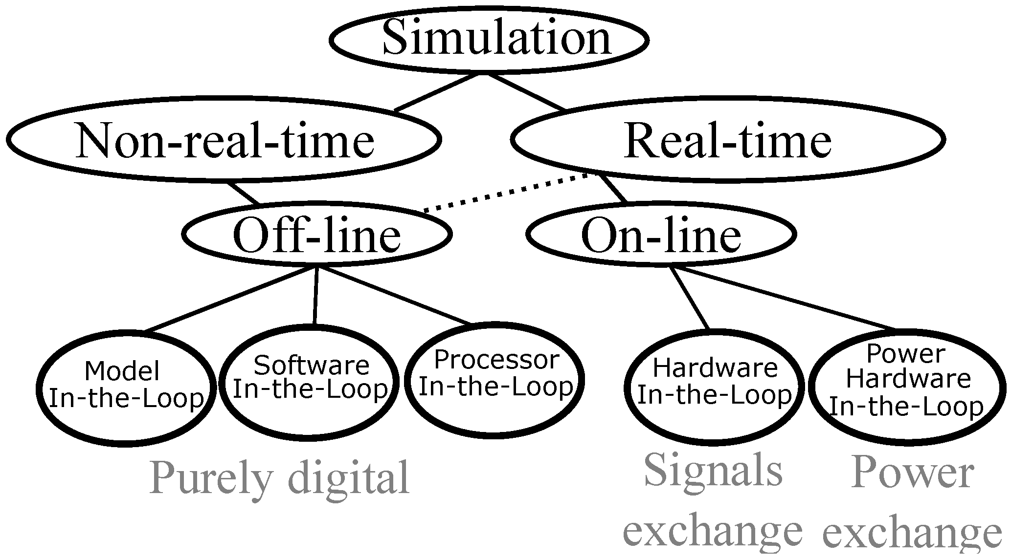
Figure 3.
Task planning example.
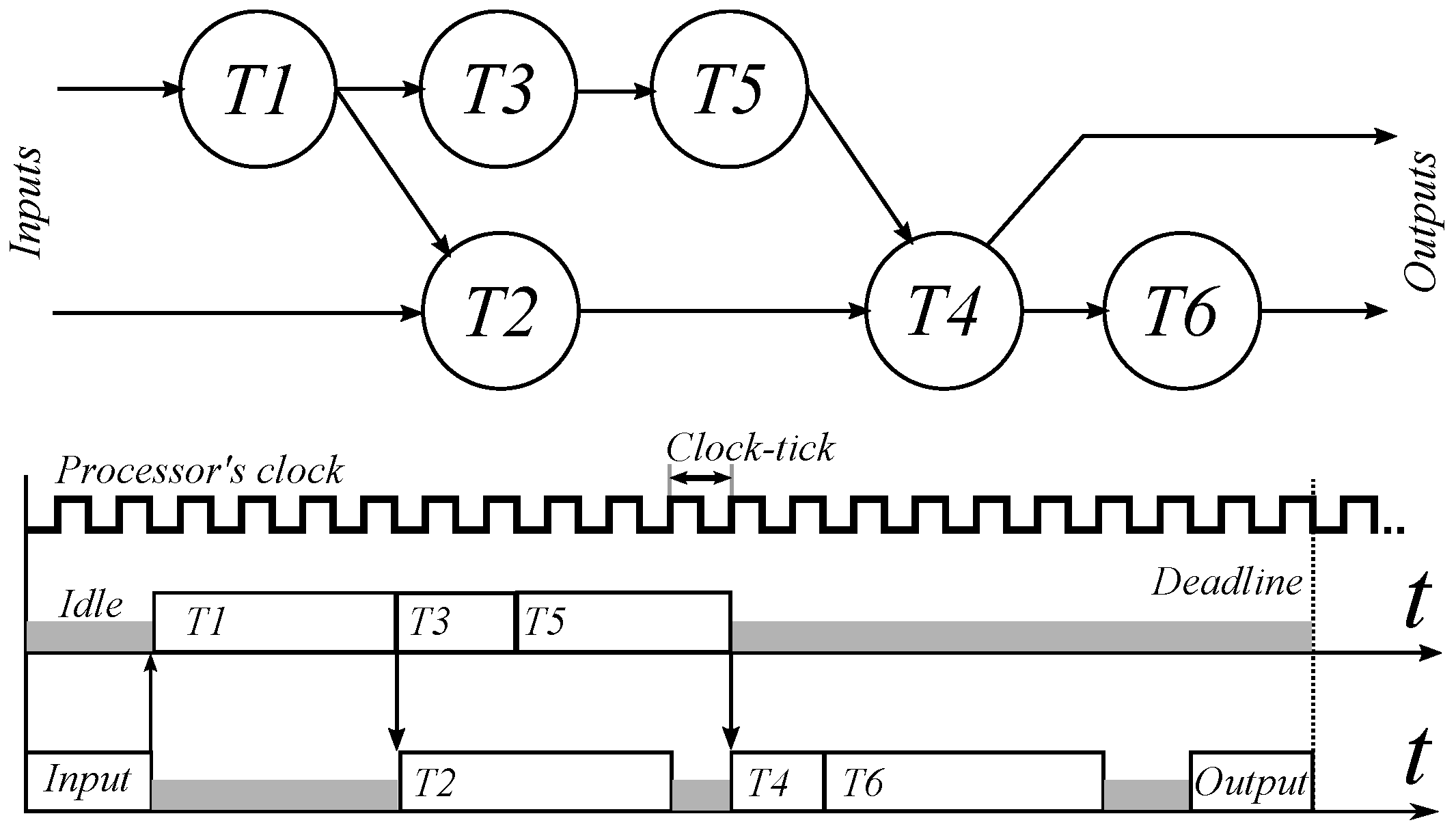
Figure 4.
Evolution of RT simulators.
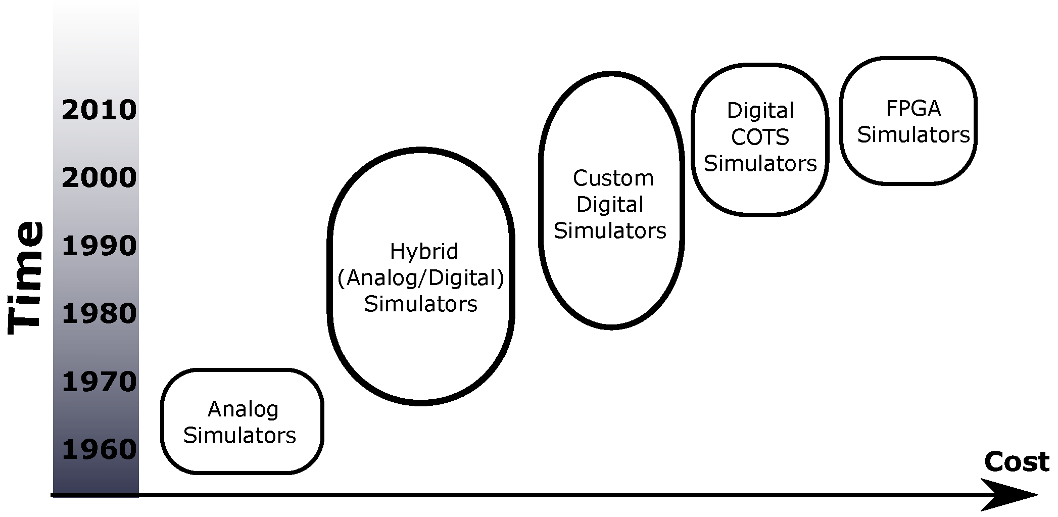
Figure 5.
An example of the P-HIL simulation.
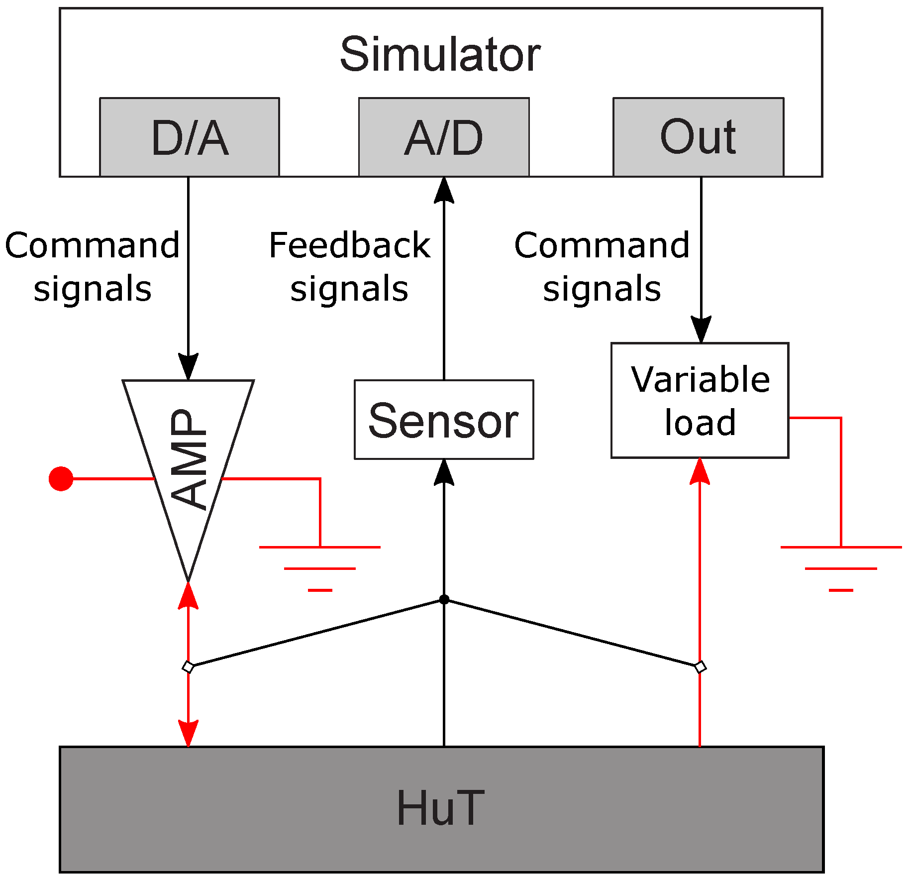
Figure 6.
Time step requirement vs. the number of nodes.
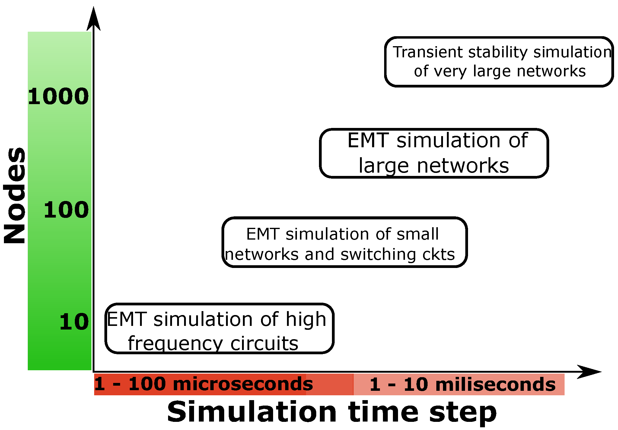

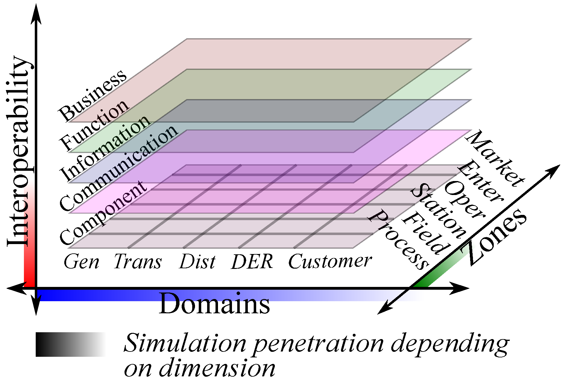
Table 1.
Real-time simulators.
| Simulator | Hardware Engines | OS | Software Compatibility | Communication, Interfacing | Applications |
|---|---|---|---|---|---|
| Opal-RT | Intel processors and FPGAs | Windows and Linux | MATLAB, Simulink, Labview | Gigabit Ethernet, PCIe with DSP-based A/C and D/A, CAN | Power electronics, control systems, HIL, power systems like smart grid |
| RTDS | NPX processor | Windows and Linux | MATLAB and Simulink | Optical fiber, Gigabit Ethernet, TCP/IP | Power electronics, control systems, HIL, power systems like smart grid |
| Typhoon | Processor and FPGA | Windows | MATLAB | Ethernet RJ45, CAN | Power electronics, control systems, HIL |
| NI Hardware | Intel processors and FPGA | Windows and Linux | Labview | Optical fiber, Gigabit Ethernet, PCI, CAN | Power electronics, control systems, HIL, power systems like smart grid |
| dSPACE | Intel processor and FPGA | Windows | MATLAB and Simulink | Gigabit Ethernet, PCIe, CAN | Power electronics, real-time control, rapid prototyping, power systems like smart grid |
Table 2.
Classification of power amplifiers [70].
Table 2.
Classification of power amplifiers [70].
| Amplifier Operation | Definition | Complexity | Types | Dynamic Response | Cost | Application |
|---|---|---|---|---|---|---|
| Linear | Output is proportional to input | Low | Voltage or current | High bandwidth and fast response time (<6 s) | High | Low flexibility (voltage or current). Difficult to build in the MW range due to high power losses. |
| Non-Linear | Output is not proportional to the input | High | Switching mode | Reduced bandwidth and slow response time (>50 s) (due to additional control circuitry) | Low | High flexibility (voltage and/or current). Commonly used in the MW range. |
Table 3.
List of power amplifiers.
| Power Amplifier | Operating Modes | DC and AC Ratings | Measurements |
|---|---|---|---|
| Ametek (Pi version) | AC, DC and AC + DC |
| AC measurements: voltage and current rms, DC voltage and current, real power, apparent power, power factor |
| Egston (CDAR200) | AC, DC |
| Current and voltage, Opal-RT integration |
| Puissance plus (PA-24K) | AC, DC and AC + DC |
| Current, voltage, power analyzer |
| Triphase (PM15A60F60) | AC, DC |
| Voltage, Currents, MATLAB/Simulink integration |
| Typhoon Power Emulator | AC, DC, AC + DC |
| Voltage, currents (using Typhoon HIL) |
| Spitzenberger Spies | AC, DC |
| Voltage, currents |
© 2017 by the authors. Licensee MDPI, Basel, Switzerland. This article is an open access article distributed under the terms and conditions of the Creative Commons Attribution (CC BY) license (http://creativecommons.org/licenses/by/4.0/).
Share and Cite
MDPI and ACS Style
Ibarra, L.; Rosales, A.; Ponce, P.; Molina, A.; Ayyanar, R. Overview of Real-Time Simulation as a Supporting Effort to Smart-Grid Attainment. Energies 2017, 10, 817. https://doi.org/10.3390/en10060817
AMA Style
Ibarra L, Rosales A, Ponce P, Molina A, Ayyanar R. Overview of Real-Time Simulation as a Supporting Effort to Smart-Grid Attainment. Energies. 2017; 10(6):817. https://doi.org/10.3390/en10060817
Chicago/Turabian StyleIbarra, Luis, Antonio Rosales, Pedro Ponce, Arturo Molina, and Raja Ayyanar. 2017. "Overview of Real-Time Simulation as a Supporting Effort to Smart-Grid Attainment" Energies 10, no. 6: 817. https://doi.org/10.3390/en10060817
Note that from the first issue of 2016, this journal uses article numbers instead of page numbers. See further details here.