
Design of a H∞ Robust Controller with μ-Analysis for Steam Turbine Power Generation Applications


1
TeCIP Institute PERCRO Laboratory, Scuola Superiore Sant’Anna, via Alamanni 13B, Ghezzano, 56010 Pisa, Italy
2
Department of Information Engineering, Università di Pisa, via G. Caruso 16, 56122 Pisa, Italy
3
General Electric Oil & Gas, via F. Matteucci 2, 50127 Firenze, Italy
*
Author to whom correspondence should be addressed.
Energies 2017, 10(7), 1026; https://doi.org/10.3390/en10071026
Submission received: 10 March 2017
/
Revised: 23 June 2017
/
Accepted: 13 July 2017
/
Published: 19 July 2017
(This article belongs to the Special Issue Energy Production Systems)
Abstract
:Concentrated Solar Power plants are complex systems subjected to quite sensitive variations of the steam production profile and external disturbances, thus advanced control techniques that ensure system stability and suitable performance criteria are required. In this work, a multi-objective robust controller is designed and applied to the power control of a Concentered Solar Power plant composed by two turbines, a gear and a generator. In order to provide robust performance and stability in presence of disturbances, not modeled plant dynamics and plant-parameter variations, the advanced features of the -analysis are exploited. A high order controller is obtained from the process of synthesis that makes the implementation of the controller difficult and computational more demanding for a Programmable Logic Controller. Therefore, the controller order is reduced through the Balanced Truncation method and then discretized. The obtained robust control is compared to the current Proportional Integral Derivative-based governing system in order to evaluate its performance, considering unperturbed as well as perturbed scenarios, taking into account variations of steam conditions, sensor measurement delays and power losses. The simulations results show that the proposed controller achieves better robustness and performance compared to the existing Proportional Integral Derivative controller.
1. Introduction
The interest in the use of renewable energy sources has grown significantly in the recent years, since the supply of fossil hydrocarbon resources is decreasing as a consequence of the growing energy demand, but especially due to the ever increasing need to reduce the relevant environmental impact of fossil-based energy systems. Solar energy is the energy source with the greatest potential of all the renewable sources [1] and it can be harvested and stored for power generation. There are two mainstream categories of devices utilized for this purpose: Photovoltaics (PV) and Concentrated Solar Power (CSP) plants. This last category is gaining an ever-increasing diffusion worldwide [2], as it offers great efficiency and is amongst the most promising cost-effective technologies for renewable electricity energy production [3].
A CSP plant generates electrical power by using different kind of technologies [4] (e.g., parabolic trough, solar towers, etc.) to concentrate a large area of solar thermal energy onto a small area of collecting surface, which exploits such energy to generate steam. Electric power is generated by means of a steam turbine connected to an electrical power generator. The main peculiarity of the application of steam turbines in CSP lies in the fact that the available solar energy shows considerable variations and oscillations due to the daily cycle of irradiation and to the weather conditions. In particular, the power generation unit may undergo a start-up and shut down cycle on a daily basis and quite sensitive variations in the steam production profile are possible during the day. The possibility of incorporating thermal energy storage or backup systems in the plant [5] and non-standard control techniques allows operating continuously.
Steam turbines were originally designed for producing energy from fossil fuels: their mechanics and their control systems are designed assuming a quite stable steam production and few start-up and shut down cycles. Therefore, the standard control techniques currently applied to turbomachinery, which are exploited also for CSP plants, are often unable to automatically adapt to changing operating conditions and cannot guaranteed the desired performance [6]. Control system parameters are set during the commissioning phase of the brand-new machine, through time consuming and effort-intensive procedures. Afterwards, such parameters are only seldom re-adjusted based on semi-heuristic procedures. This implies the machine to work in non-optimal efficiency conditions during its lifetime. The control procedures need to allow correct and efficient operation of the turbomachine also in transient conditions and without compromising its integrity.
CSP plants exhibit large variations of steam features, nonlinearities, different sources of uncertainties, characteristics that result in detuned performance with classical Proportional Integral Derivative (PID) control [2]. Hence, the main purpose of this work is to study the application of advanced control techniques that can cope with these issues, focusing on CSP plants application and typical power loading profile. The turbine control with variable operating conditions can be addressed by investigating the applicability of several advanced control strategies. Adaptive control approaches, which are capable to adapt gains in different loading conditions and uncertainties are known. Examples of these kind of strategies were presented in [7], where a Model-Reference Adaptive Controller (MRAC) was applied to a non-linear boiler-turbine unit with parametric uncertainties, and in [8], where an improved adaptive backstepping method was designed to control a turbine speed governor system with parametric uncertainties and exogenous disturbances. In the field of robust control, control has received relevant attention in the scientific and technical community and has been widely used for industrial applications. Through its design philosophy, the approach improves in an optimal way the robustness of the control system. Examples of robust controller based on loop-shaping or mixed-sensitivity design were proposed in recent studies [9,10]. In particular, two robust Multiple-Input Single-Output (MISO) controllers were developed and designed by setting out a mixed sensitivity problem in [9], while an output tracking control system for improving the load-following capability of a boiler-turbine unit by using feedback linearization and loop-shaping method was presented in [10]. An application of control technique coupled with the structured singular value analysis and synthesis was presented in [11]. In [12] an controller was applied to a boiler-turbine system modelled through Fuzzy technique. Predictive control approaches have been investigated in [13], where a linear Model Predictive Control (MPC) controller was proposed for a derived nonlinear model of a steam turbine solar power plant, and in [14], where the General Predictive Control (GPC) and Constrained Receding-Horizon Predictive Control (CRHPC) were exploited for the control of large steam turbines during load variations. In addition, intelligent control approaches were addressed through the control of steam turbines. For instance, in [15,16] fuzzy logic was used in order to adjust on-line the gains of a PID controller. In [15], a steam turbine governing system was controlled through a non-linear self-adaptive fuzzy PID controller adopting fuzzy rule and inference to adjust the PID parameters, while in [16] a fuzzy gain scheduled proportional and integral was applied to the power plant. In [17], a feed-forward controller, whose core is a neuro-fuzzy-based Hammerstein model, was employed to control a boiler-turbine unit and artificial intelligence (AI) methods were adopted in [18,19,20] in order to adjust the parameters of a PID controller. In particular, fuzzy, Genetic Algorithms (GA), Particle Swarm Optimization (PSO), and Adaptive Neuro-Fuzzy Inference System (ANFIS) techniques were compared in [18], PSO was used in [19], PSO combined with radial basis function neural networks (RBFNN) algorithms were exploited in [20] and GA were applied in [21]. In addition, Model-Based Control (MBC) schemes, such as Feedback Linearization and Linear Quadratic Regulator (LQR) were investigated for the control of a two-stage steam turbine [22], and Internal Model Control (IMC) with a cascade PID controller was adopted in order to control the superheated steam temperature system [23]. All control techniques provide good results in turbine power applications. Methods like adaptive control or MPC have the main drawback of a considerable computational cost due to their variable structure. A fuzzy logic controller, which extends the simplicity of PID and adapts the control action at actual operating condition using knowledge and experience on the system behavior, has already been developed in [24]. Robust control was selected, as it provides a parametric solution in presence of uncertainties, it yields a structure that is easy to implement on a Programmable Logic Controller (PLC) and is characterized by a low computational cost. The controller design can be automated through a numerical procedure by using the available software [25] and it relies on validated linear approximations of the system model, which cover the majority of the operating envelope of the plant itself. A typical drawback of the proposed approach is represented by the controller order, which is typically high. However, it is possible to reduce the order of original controller with moderate degradation of robustness and performance of the feedback system.
This paper presents a multi-objective robust controller implemented with a signal-based approach [26]. The purpose of this work is to show the applicability of the control approach and the structured singular value tool in the context of renewable energy systems, in particular on the CSP plants. The strategy can be applied to Multiple-Input Multiple-Output (MIMO) systems and allows designing a controller that stabilizes the plant and minimizes a fixed cost function. The signal-based design is similar to mixed sensitivity design and provides tool for incorporating the desired control requirements in the form of well-known frequency response shaping. This technique allows achieving good nominal stability margins and performance in terms of disturbance rejection, set point tracking and limit of the control effort. In order to improve robust stability and robust performance, the structured singular value analysis (-analysis) [26,27] was performed. The proposed method is compared to the current PID-based governing system. The design of the multi-objective robust controller as well as the simulation tests were performed though the Matlab/Simulink® environment.
2. Steam Turbine Power Plant Control System
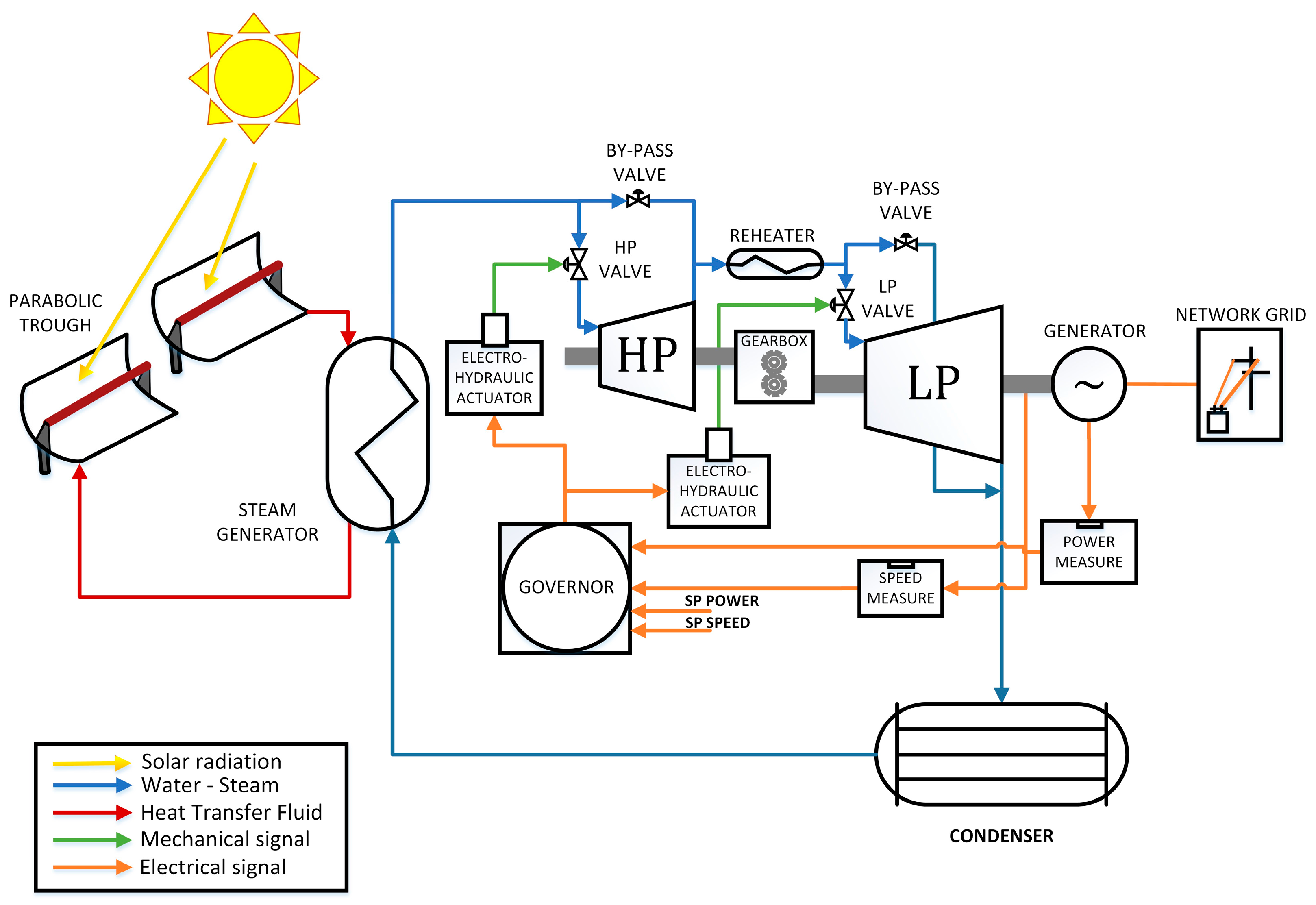
The complex of turbines considered in the present work is composed by a non-condensing high pressure (HP) steam turbine, coupled with a gearbox, a condensing low pressure (LP) steam turbine, a steam re-heater and a 55 MW electric generator. The system is completed with a condensing system receiving the exhaust steam at the LP turbine outlet and two steam by-pass systems. The governor is the main controller of the steam turbine machine and is responsible of the unit operation. The electro-hydraulic system controls the inlet valves of each turbine. Figure 1 shows a scheme of the involved system.
Many studies have been performed on the modeling of the steam turbine power plants for control, monitoring and optimization purposes. In [28], an overview of models for turbine-governor were analyzed and provided with particular attention to the behavior during the transient operations, to the frequency control and stability. A steam turbine simulation model based on thermodynamic principles and semi-empirical equations was described in [29], where the related parameters were adjusted by applying GA based on experimental data obtained from field experiments for control purposes. A hybrid thermodynamic method and a neural network approach for on-line monitoring applications were recently presented in [30].
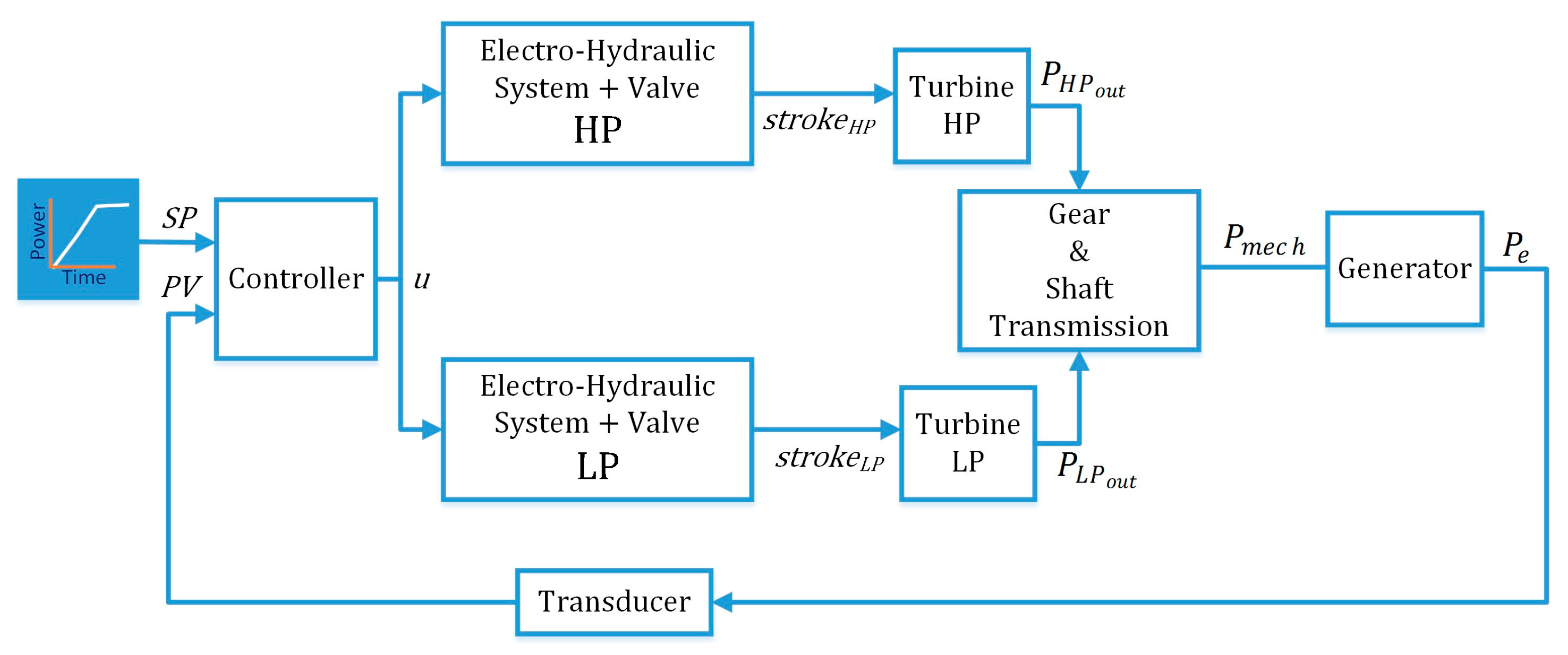
The model developed in the present work is focused on the steam turbine power control taking into account the variability in the steam header system of the considered CSP plant application. The power control model is schematically depicted in Figure 2. The generator is synchronized and connected with the grid, the by-pass valves are ramping to closure and the governor must follow a demand of power ramp. In particular, the power reference is varied from a minimum power value to a maximum one and, finally, achieves the power shutdown value under normal conditions. In this scenario, the overall control system is a cascaded controller mainly composed of an outer power loop and an inner valve stroke loop. The former one has the task to follow a demand of power and to request a control signal demand to the inner loop. This latter one has the task to control the oil pressure of the electro-hydraulic system and to follow a demand of valve stroke.
2.1. System Model
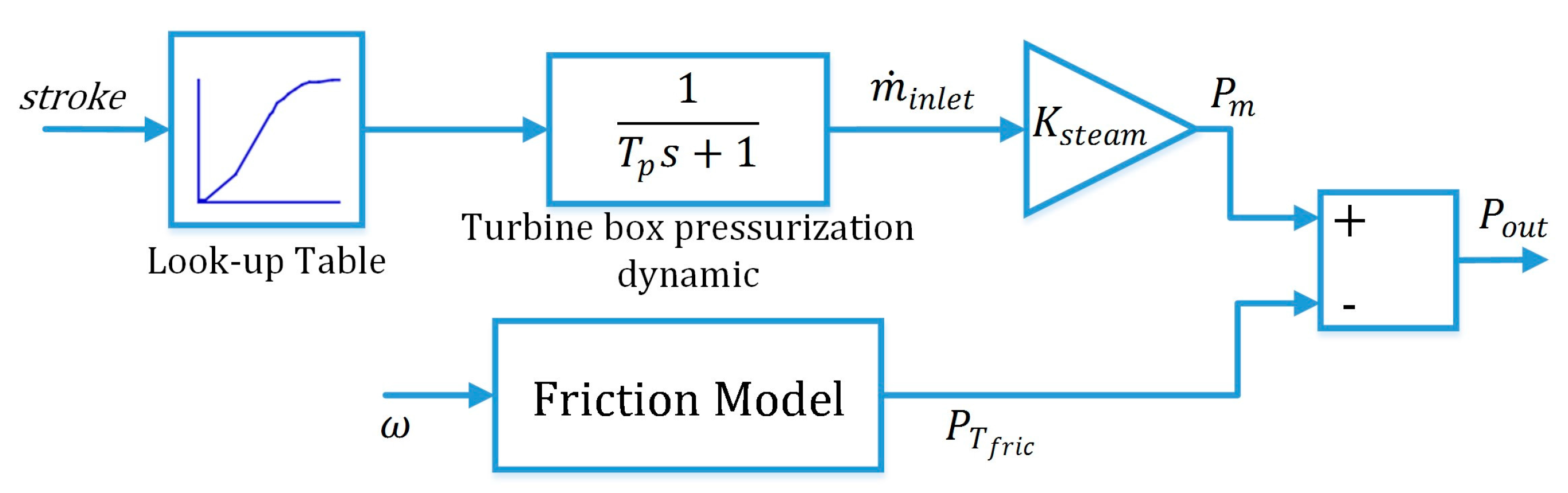
The system depicted in Figure 2 was described through a complex non-linear model developed in the Matlab/Simulink® environment. Both the steam turbines models are composed by a block that computes the inlet steam mass flow as a function of control valve stroke, a steam gain , that provides the characteristics of the flow rate and power of steam, and a friction model, which evaluates the friction power losses as function of shaft rotational speed . Figure 3 shows the Simulink model of both turbines.
The inlet steam mass flow is computed by means of a simplified model with dynamics characterized by a transfer function of the first order and a lookup table calibrated with a steam at rated conditions. can be expressed as:
where is a corrective factor that takes into account the actual condition of the steam and its value changes between 0 and 1, is the rated power and is the maximum steam mass flow.
The turbine mechanical drive power is computed as:
The useful power output can be described as:
where is defined as:
with being the bearing power losses at the rated synchronous speed .
The gearbox and the electric generator are modelled by taking into account all the possible additional power losses of the train. The gearbox model computes the balance of the power acting on the LP shaft. In particular, it is assumed that both torques and angular velocities are reported at the same LP shaft. The angular velocity is computed through the balance of both HP and LP turbine torques and , the electric generator torque and the gearbox friction torque ; it is integrated and divided by the total moment of inertia acting on the LP shaft , according to the Equation (5):
where:
The gearbox friction torque is equal to the sum of two contributions, one due to windage and bearing friction and the other one due to full load power losses , and is computed as:
where are the rated windage and bearing power losses, are the full load power losses and is the maximum value reached by the HP turbine torque. The electric generator model computes the generated electric power as the useful mechanical power at generator shafts minus the gearbox power losses and electrical and mechanical losses on the electrical generator :
The complex hydraulic parts of both HP and LP electro-hydraulic actuators and related valves were modelled with the Simscape Toolbox of Matlab®/Simulink. The electro-hydraulic system is composed by a current to pressure converter (CPC), which controls the hydraulic pilot cylinder (HPC) movements. The HPC allows the passage of the volume oil flow to the chamber of the hydraulic double acting cylinder (HDAC), which controls the input valve position of the steam turbines. A detailed scheme of the electro-hydraulic system is depicted in Figure 4. The parameters of the hydraulic components modeled were derived from schemes and datasheets provided by General Electric Oil & Gas.
The Governor is a non-standard Proportional-Integral (PI) controller, hereafter also called PID Governor, with the task of following a demand of power and to request a control signal demand to the actuators. The controller software is property of General Electric Oil & Gas and has the following three main features:
- An anti-windup obtained by differential formulation of the integral component.
- limiter in the output.
- proportional gain involved as well in the integral component calculation.
Finally, power transducers and filters are also represented by transfer functions.
3. H∞ Controller for Steam Turbine Power Control
For the power control loop, a multi-objective robust controller was selected and implemented. In this section, the robust control problem statement and design are presented.
3.1. Problem Statement
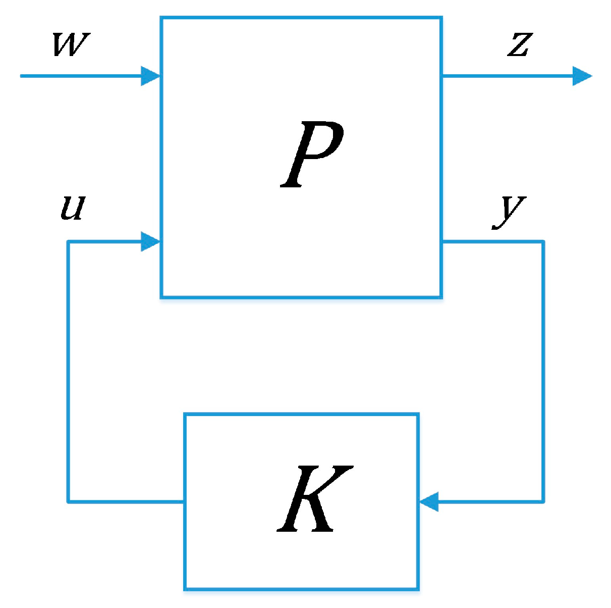
Let us consider the general plant represented by the transfer matrix and the control system configuration shown in Figure 5.
The plant has two inputs and two outputs:
- the generalized disturbance , which cannot be affected by the controller and includes references, disturbances and noise signals;
- the output signal of the controller called control input;
- the input signal of the controller called measurement output;
- the controlled variable , which denotes the performance requirements.
The open loop interconnection can be generally described by the equations system:
where is partitioned in 4 main subsystems.
The closed-loop system is given by the Lower Linear Fractional Transformation (LLFT) of and , denoted by :
The -optimal control problem [26] consists in finding all stabilizing controller that minimize the cost function:
where is the -norm defined as:
with the maximum singular value of . The direct minimization of is a very hard problem and finding the optimal controller is difficult; therefore a sub-optimal problem is solved and conditions to ensure the existence of a stabilizing controller are found. Let be the minimum value of over all stabilizing controllers . The sub-optimal problem consists in finding all stabilizing controller such that , for a given . There are two main methods for solving this sub-problem:
- Riccati equations approach.
- Linear Matrix Inequalities (LMI) approach.
A discussion of Riccati solution was presented by Doyle et al. in [31], while a LMI solution was presented in [32,33].
If a controller that achieves is desired, to within a specified tolerance, then it can be performed a bisection on until its value is sufficiently accurate. This procedure is called -iteration and allows finding the minimum of with any degree of accuracy.
3.2. Optimization
The control variable denotes the performance requirements of the system. The performance objectives of a feedback system can usually be specified in terms of requirements on the sensitivity , complementary sensitivity and control effort functions:
where is the nominal plant and is the controller.
The mixed sensitivity approach (which is schematically represented in Figure 6) provides the design goals by acting on the previous functions with weights in form of desired frequency response shaping.
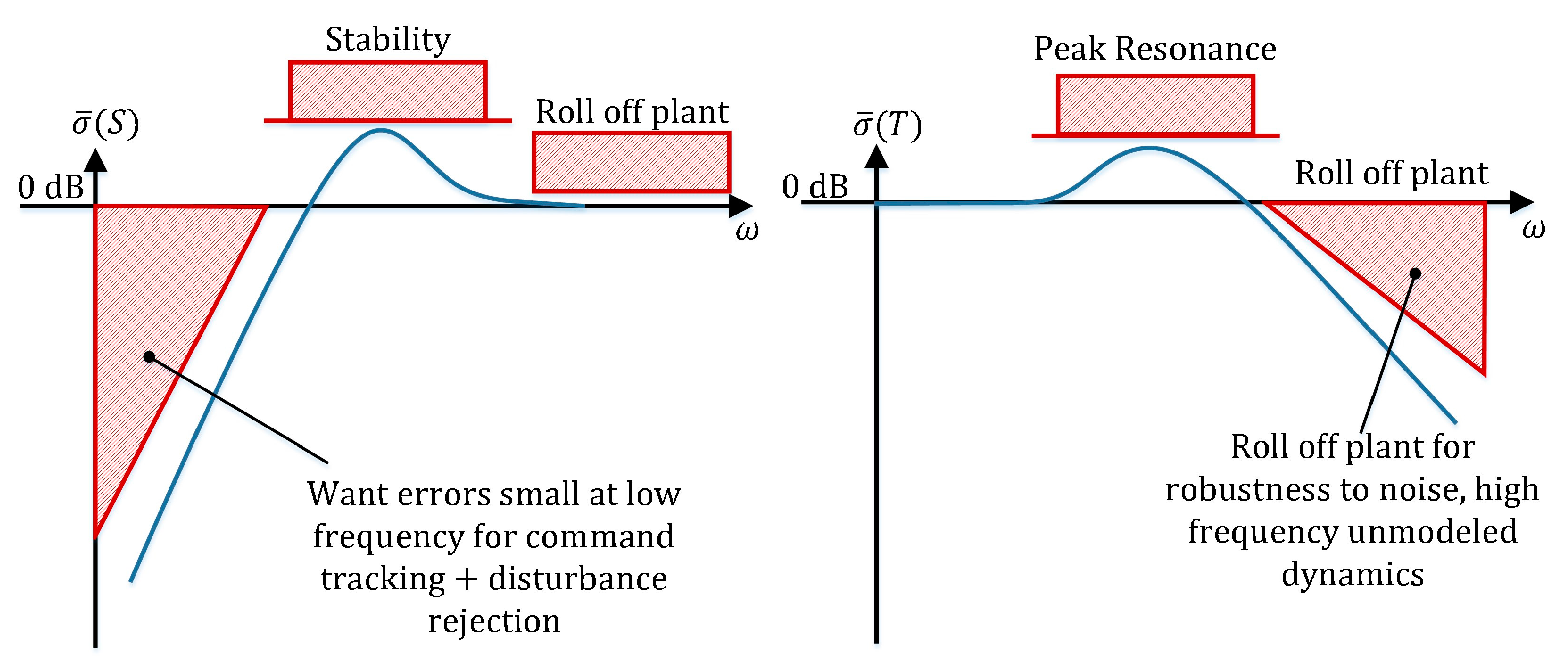
In order to get small control errors and good disturbance rejection, penalize large inputs and attenuate noise signals, the maximum singular value of the sensitivity function , of the control effort and of the complementary sensitivity , must to be bound, such as depicted in Figure 7. In particular:
- needs to be minimize over the low-frequency range to get small tracking error and good disturbance rejection. This specification may be captured simply by an upper bound of , where has low-pass filter characteristics with bandwidth equal to the bandwidth of the disturbance.
- needs to be minimized at high frequencies to account for noise and unmodeled dynamics that appear in that frequency range. To achieve this goal, one might specify an upper bound of , where has high-pass filter characteristics.
- should be kept at low values to limit the control signal in order to prevent saturation of the actuators. This specification may be captured simply by an upper bound of , where has high-pass filter characteristics or is constant.
These requirements may be combined into an -problem, which is defined as:
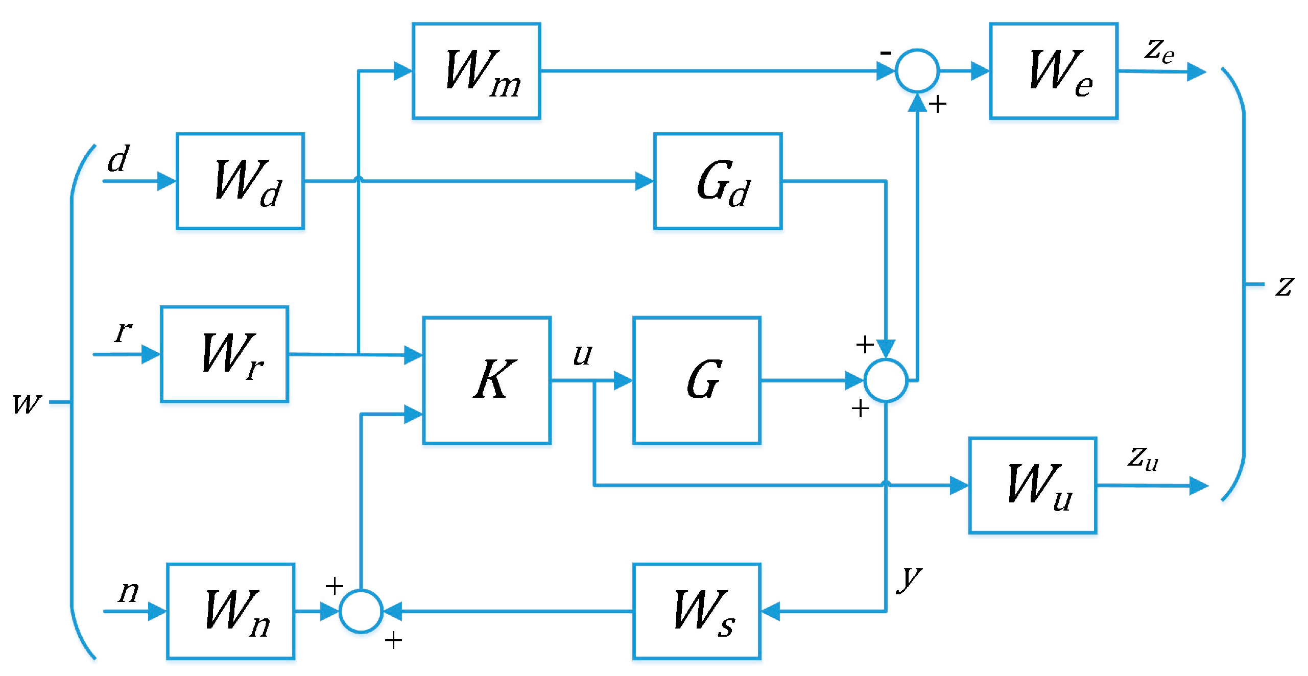
Instead of shaping the basic transfer functions, it is possible to work with the so-called signal-based approach [26] shown in Figure 8. The meaning of the weights are as follows:
- forms the frequency content and magnitude of the exogenous disturbance affecting the plant.
- shapes the magnitude and the frequency of the reference command.
- represents the frequency-domain models of sensor noise.
- represents the desired model for the closed-loop system with tracking.
- shapes the tracking error.
- forms the frequency content and magnitude of the control signal use.
- represents the model of the sensor dynamics. This model might also be lumped into the plant model .
It is straightforward to show that:
with and .
This objective is similar to the usual mixed sensitivity optimization. The weighting functions are used to scale the input/output transfer functions such that .
3.3. Linear Model Description
For the control purposes, a linear approximation model of the system was considered. Taking into account the model developed in the Section 2.1, the linear model was obtained with the following assumptions:
- Offsets as well as saturations were eliminated.
- A linear model of the electro-hydraulic system with the valve of both HP and LP turbine was identified and introduced as transfer function. Since the dynamic of the system must take into account several dynamic components and the delay due to the oil flow, the system was identified with a fourth-order, stable and not minimum phase transfer function with the structure:
The presence of a nonminimum phase zero in (18) limits the amplification of the loop gain and the general performance. This is however independent of the controller used.
The goodness of fit between the linear and the real model was valuated using the Normalized Root Mean Square Error (NRMSE) cost function defined as follows:
where ‖∙‖ is the 2-norm of a vector, is the vector of the real model output subjected to different input step command and is the vector of the estimated model output.
- The nonlinearities introduced by the look-up tables were replaced by constant gains defined as the ratio between the maximum inlet steam mass flow and the maximum stroke valve:
The linear model of the system is depicted in Figure 9, where represents the transfer function of the controller, and the transfer functions of the main elements of the turbine power system.
3.4. Derivation of Uncertainty Model
The design of robust control methods allows the incorporation of uncertainties in the plant model. Not modeled dynamics of actuators, sensors and turbine plant-parameter variations are the common uncertainties of the system. In the next subsections a representation of these kind of uncertainties is presented, for the process considered in this work.
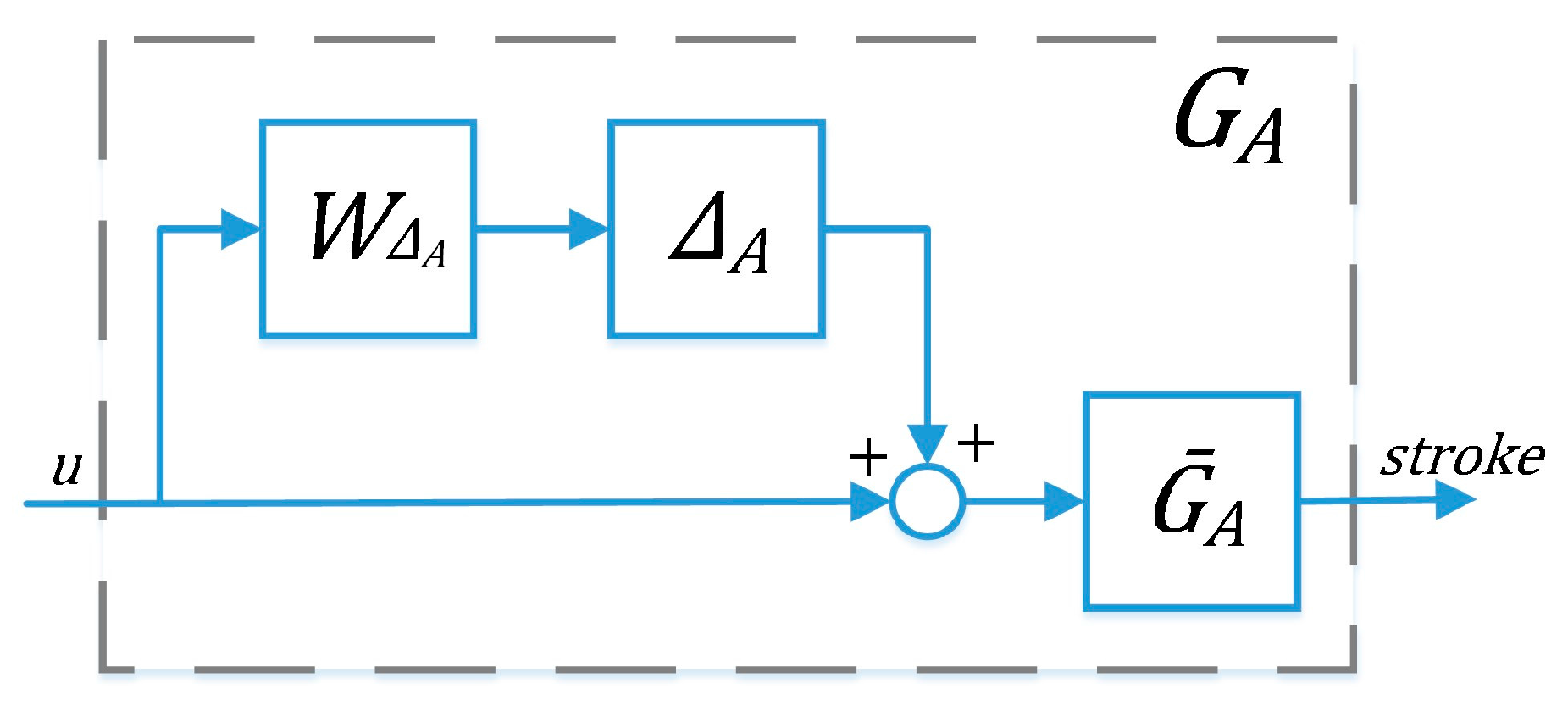
3.4.1. Actuator System Uncertainties
In order to take into account the unmodeled dynamics of the valves actuation system, the uncertainties in the actuator models are approximated by input multiplicative uncertainties as shown in Figure 10.
The perturbed system is described as:
where is the nominal transfer function of the electro-hydraulic system with valve (Equation (18)), the unknown uncertainty stable and norm bounded () and the weight uncertainty defined as:
The unmodeled dynamics uncertainty is somewhat less precise and thus more difficult to quantify. Therefore, the simplified form of the previous equation is usually adopted [26], where the value represents the percentage of the modelling error at low frequency while the percentage error at high frequency. The 100% uncertainty in the model occurred when the weight function achieves a magnitude value of 1, approximately at the value of . The weighting functions considered here were derived according to the nominal transfer function and the bandwidth of the actuators, taking into account a good model of these latter ones at low frequency. The multiplicative weights are described as:
3.4.2. Turbine Parameter Uncertainties
The main parameter variation of the turbines is due to the actual condition of the steam. It is related to the heat profile during the day. The variation of the steam condition can be represented by a parametric uncertainty:
where is the nominal value, represents the percentage of variation and is a real parameter bounded (. It was observed from the experimental data that, in a typical day where the weather conditions are quite good, the turbine power is on average 70%, and for the 80% of the time, the power lies in the range [50%, 100%]. Therefore, the values 0.77 and a 30% were selected for and for HP and LP turbines, respectively.
A representation of the turbine block with separated uncertain parameter using the Upper Linear Fractional Transformation (ULFT) of and , denoted by , is shown in Figure 11a, where
with:
3.4.3. Sensor Parameter Uncertainties
The time constant of the sensor is another uncertain parameter of the actual system. The inaccuracy of the sensor time constant can be represented by a parametric uncertainty:
where is the nominal value, represents the percentage of variation and is a bounded real parameter (. It was observed from the site data that the data transmission delay lies between 0.5 and 1.5 s. Thus a value of 1 and a 50% of tolerance were chosen for and , respectively. Clearly, the amount of tolerance used may produce a more conservative design, but this is coherent with typical worst case operating point(s) used in classical PID control.
A representation of the sensor block with separated uncertain parameter using the ULFT is shown in Figure 11b, where:
with:
3.5. Performance Specifications
The designed control system must achieve good disturbance rejection and noise attenuation, as well as good tracking error; therefore, performance weights must be selected. Finding appropriate weighting functions is a crucial step in robust control design: there must be a trade-off between the nominal performance and robust performance of the closed loop system and their selection usually involves trial and error procedures.
A signal-based approach was adopted for the optimization and the following main weight functions were defined:
- forms the frequency content and magnitude of the exogenous disturbance affecting the plant.
- represents the frequency domain model of the sensor noise.
- is an ideal model of performance, to which the designed closed-loop system tries to match.
- represents the control action constraint.
- introduces the constraints on the maximum stroke of both HP and LP valve.
- shapes the error between the response of the close-loop system and the ideal model .
Figure 12 shows the block diagram of the closed-loop system, which includes the feedback structure and the controller as well as the elements representing the model uncertainties (highlighted in green) and the performance objectives (highlighted in orange).
The generalized disturbance of the system consists of the reference input (), the input disturbance (), and the noise (), while the vector of performance requirements is composed by the control variables , (is a vector of two components) and :
The system uncertainties can be separated from the model and grouped into a diagonal structured block norm bounded with input and output :
The signal is the controller output, while the input of the controller consists of the reference signal and the measured electrical power , which is affected by noise:
Now, the defined weight functions will be described, and the performance objectives will be discussed in the next section.
3.5.1. Disturbance Weight Function
In the power control scenario the different power losses are constant and are introduced in the system by the vector weight function .
The input disturbance of was considered as a step signal.
3.5.2. Noise and Control Action Weight Functions
The noise shaping function is determined on the basis of the spectral content of the sensor noise signal and usually has its peak value at high frequency because the noise is mainly concentrated at high frequencies. In this contest, the noise shaping function was modeled with a constant function due to the lack of sensor technical data, considering a worst-case design, where the power spectral density of the noise signal is constant for all frequencies. However, the robust control design structure derived with the assumed can be refined if better statistics become available. The input noise of was considered as a zero mean Gaussian white noise.
In order to avoid actuators saturation, it is necessary to have a control action smaller than a constant value. Therefore, the normalizing weight function is taken equal to unity.
3.5.3. Stroke Valve Weight Function
In order to avoid exceeding the maximum stroke (100%) of both HP and LP valve, constant bounds are introduced by means of the weight function , which is defined as:
3.5.4. Closed-Loop Ideal Model Weight Function
is an ideal model of performance, which the designed closed-loop system tries to match. The model transfer function is selected so that a set of performance indexes adapted to the input power ramp reference shown in Figure 13 are satisfied. Such indexes are settling time (time elapsed from ramp command start to actual power within ±5% of target value), rise time (time elapsed from ramp command start to 90% of target value), overshoot (the maximum peak value measured from the target value) and integral absolute error (IAE, evaluated along the entire ramp), which is defined as:
where is the tracking error between set point and actual value.
The set-point specifications constraints defined by the company are the following:
- Settling time <141 s
- Rise time <131 s
- Overshoot <2%
- IAE < 4104
For a good tracking of reference signal, a second order well-damped system has been selected:
where is a desired natural frequency and a desired damping ratio.
A model satisfying the above mentioned requirements is:
3.5.5. Tracking Error Weight Function
The difference between the response of the closed loop system and the ideal model is reflected in the weight function . The aim of this weight is to achieve a small difference between the system and model output and a small effect of the disturbance on the system output. The form of is usually a high-pass filter [26], but the selection of the appropriate parameters is not simple, as it should represent a trade-off between nominal and robust performance. Therefore, two types of function were tested, namely a transfer function of the first and second order, with one or two zeros, respectively. The performance weighting function expressed by the Equation (37) was obtained through a trial and error approach, evaluating the nominal performance and the robust performance of the control system, and preferring a simple structure:
If one needs to enforce the performances (e.g., the rise time condition) both numerator and denominator coefficients of have to be increased by shifting the weighting frequency response toward higher frequency values.
3.6. Control Synthesis
The controller synthesis problem is to find a linear, output feedback controller that has to ensure the following properties of the closed-loop system:
- Nominal Performance:where is the unperturbed open-loop system and ‖∙‖∞ is the -norm.
- Robust Stability:for structured uncertainty where is the structured singular value, corresponding to the transfer matrix from to , the so called matrix .
- Robust Performance:for the structured uncertainty where is the structured singular value, corresponding to the transfer matrix from to , the so called matrix , with regard to where is a fictitious 34 complex uncertainty block.
- Low-Order Controller:where is the full order controller and is the reduced order controller.
3.6.1. Nominal Performance Analysis
The sub-optimal problem was solved through the command “hinfsyn” of the Robust Control Toolbox of Matlab®. The interval of -iteration was chosen between 0.1 and 10 with tolerance 0.01. The synthetized controller has two input and one output and is of 35th order. The value of at the end of the -iteration is equal to 0.5051 as shown in Figure 14. Therefore, Equation (38) is satisfied and nominal stability and performance are guaranteed. The performance of the controller could be improved acting on the performance weighting functions, but a faster time-response and consequently, a larger closed-loop system bandwidth, reduce its robust performance, thus the controller was not improved.
The set-point following performance indexes are synthetized in Table 1. The power tracking of the closed-loop system is shown in Figure 15. The input disturbance in the initial stage of the power ramp is quickly rejected and the reference tracking is good. The behavior of the error when the closed-loop system tries to match the ideal model , the control action, and the stroke valve of both HP and LP turbine are shown in Figure 16. The model error is small and the constraints on control signal and stroke valves are respected, thus the performance objectives are satisfied.
3.6.2. Robustness Analysis
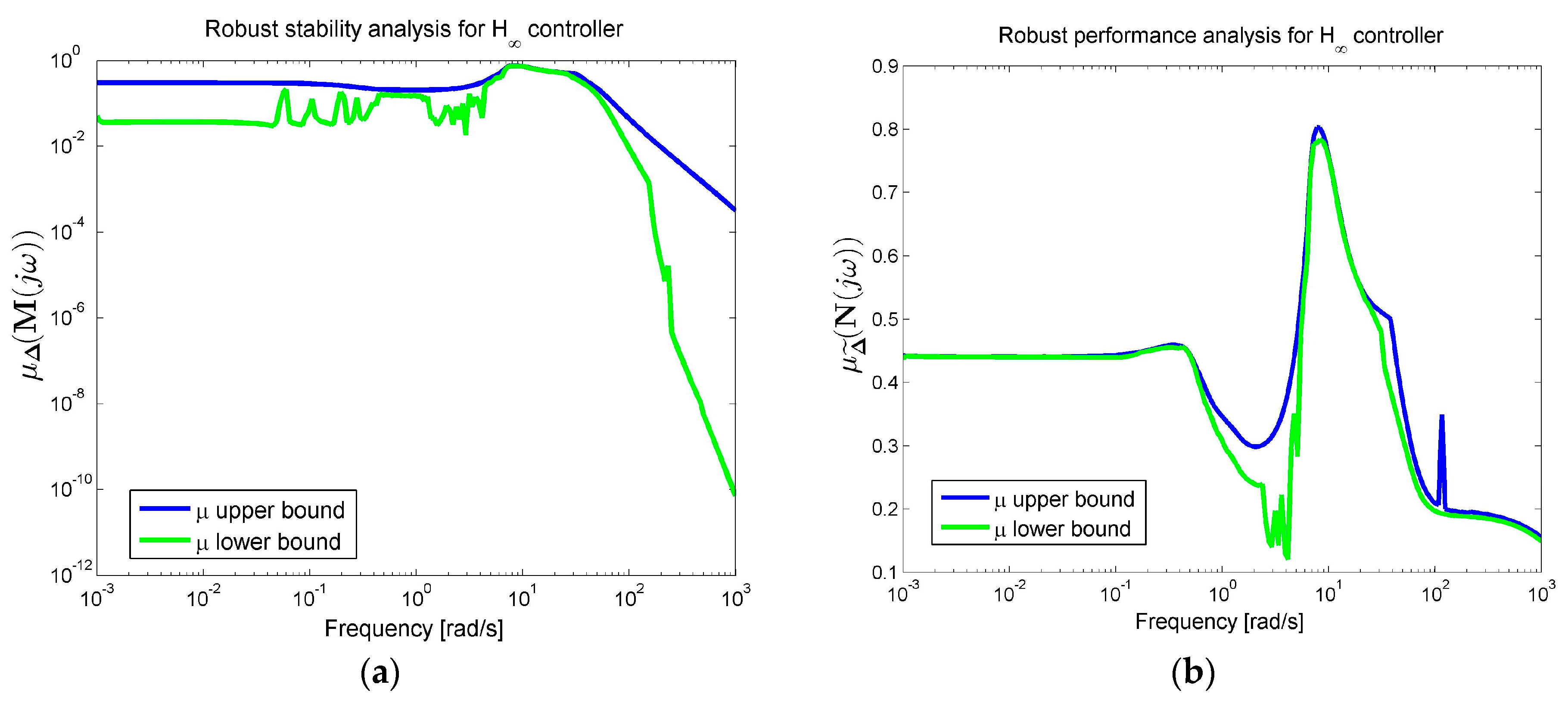
The robust properties were checked by exploiting the theory of structured singular value () [26,27]. For robust stability and performance the frequency responses of and must be computed, and its supremum evaluated, since robustness to the largest expected uncertainty set requires to be less than one.
The -analysis can be performed through the command “mu” of the Robust Control Toolbox of Matlab®. The function mu computes upper and lower bounds for the structured singular value with sufficiently high accuracy in our problem. For practical purposes, the evaluation of was carried out in the frequency range [0.001, 1000] rad/s. The structured singular value of both and are depicted in Figure 17.
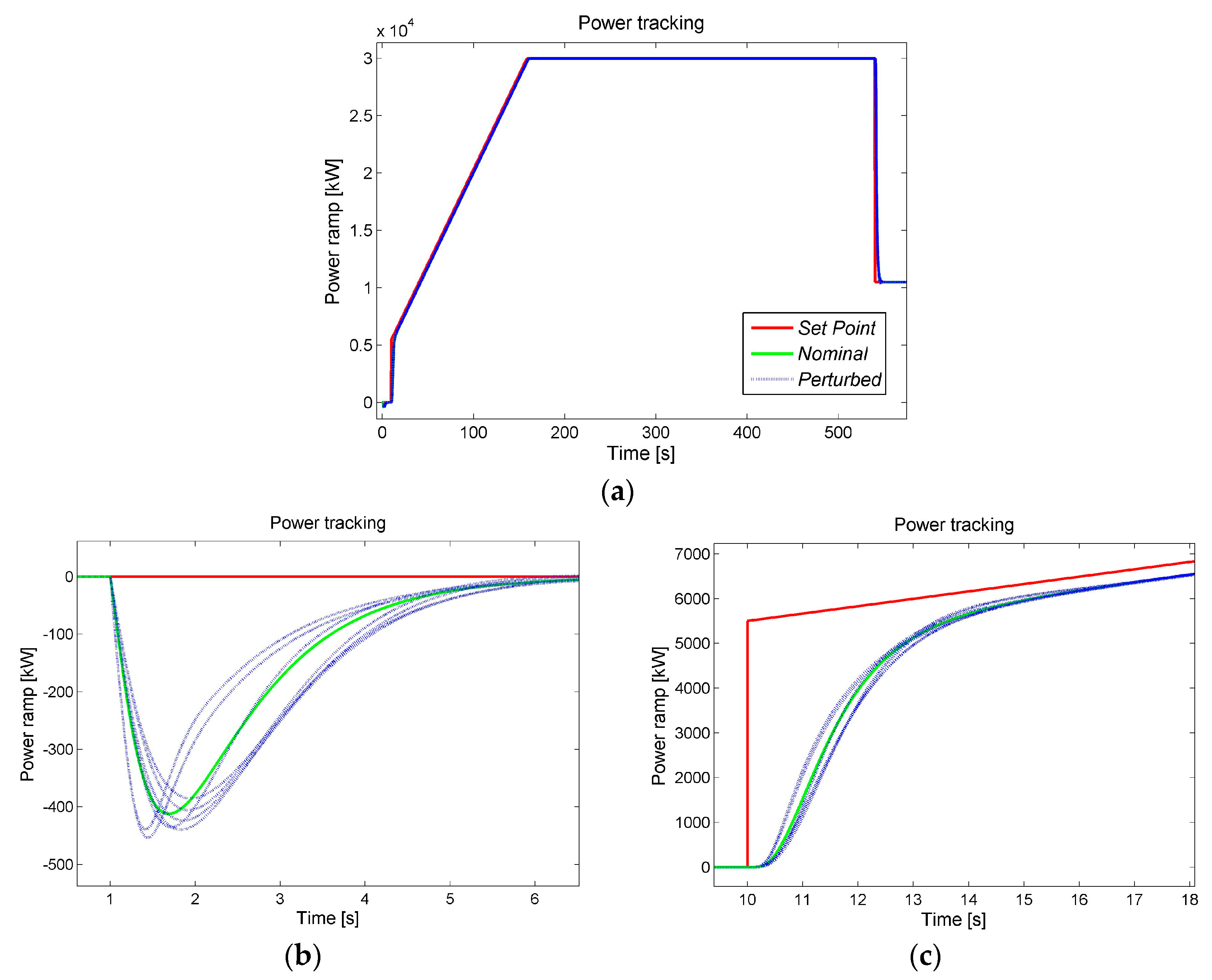
The maximum values of the upper bound for the structured singular vale of both matrices and with respect of uncertainties are 0.76 and 0.8, respectively: such values are lower than one, thus Equations (39) and (40) are satisfied and the controller guarantees robust stability and performance. The power tracking of the closed-loop system with some random samples of the uncertain system is shown in Figure 18.
3.6.3. Controller-Order Reduction
A high order controller was obtained from the process of synthesis. In order to implement a controller which is easy to handle by a PLC and is computationally less demanding, the controller order must be reduced. There are different techniques in the literature to reduce the controller order. The most commonly adopted ones are the Balanced Truncation and the Hankel-Norm Approximation. A detailed discussion of these techniques is provided in [27]. In the present work, the Balanced Truncation was applied.
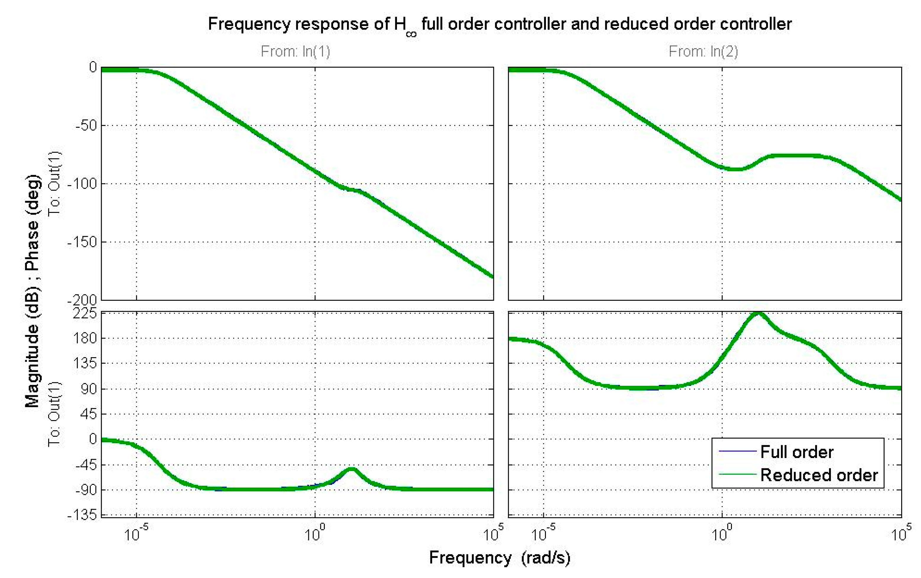
The reduced order controller was selected by evaluating the approximation error according to the Balanced Truncation method and comparing the nominal and robust performance of the obtained controllers. Controllers with order greater than 4 provided a small approximation error and similar nominal as well as robust performance with respect to the full order controller, while further reduction of the controller order led to deterioration of the control system performance. The fourth order controller was selected, as it represented a good compromise between performance and an easy implementation. In effect, an approximation error (see Equation (41)) of 3.477110−6 is satisfactory for the considered process; the nominal performance is very similar to the one of the full order controller, such as shown in Table 2, as well as the robustness analysis, which reports the same values of the full order controller. The Bode plots of full order and reduced order controller are shown in Figure 19. The corresponding plots practically coincide with each other, which implies similar performance in the closed-loop system. The low pass and band pass nature of the controllers in channel 1 and 2 is also evident in the Figure 19.
4. Simulation Results
The designed multi-objective robust controller was compared to the current PID-based governing system. The reduced order controller was discretized through the bilinear transformation (or Tustin transformation) technique before being introduced into the system, as it was assumed that it is implemented on a PLC. The discrete-time multi-objective robust controller is taken herefater as reference for the simulations. The nonlinear system was simulated with the two controllers and three experiments were performed for each tuning set:
- Nominal conditions with the typical power ramp reference.
- Perturbed conditions with a variation in steam conditions causing a 30% power reduction of turbines, a sensor dynamic slower of about 50% and added power losses of about 50% with respect to the nominal case, when the typical power ramp is demanded to the system.
- Perturbed conditions with an unexpected variation of the actual conditions of the steam (as depicted in Figure 20), which causes a gradual power reduction of turbines of about 30% during the tracking of power reference.
The results were compared assuming two scenarios corresponding to two different tuning set of the PID Governor: in the first scenario the actual PID gains, as set on the site under study, are considered. In the second scenario it is assumed that the PID Governor is optimally tuned according to the criterion of the minimum IAE [35]. Although this type of tuning is not applied during the commissioning phase on site, it can be considered a “theoretical limit” for the performance achievable through a PID and for this reason is taken as reference for the assessment of the potential advantages of the other less traditional control approaches.
4.1. Nominal Conditions with Typical Loading Ramp
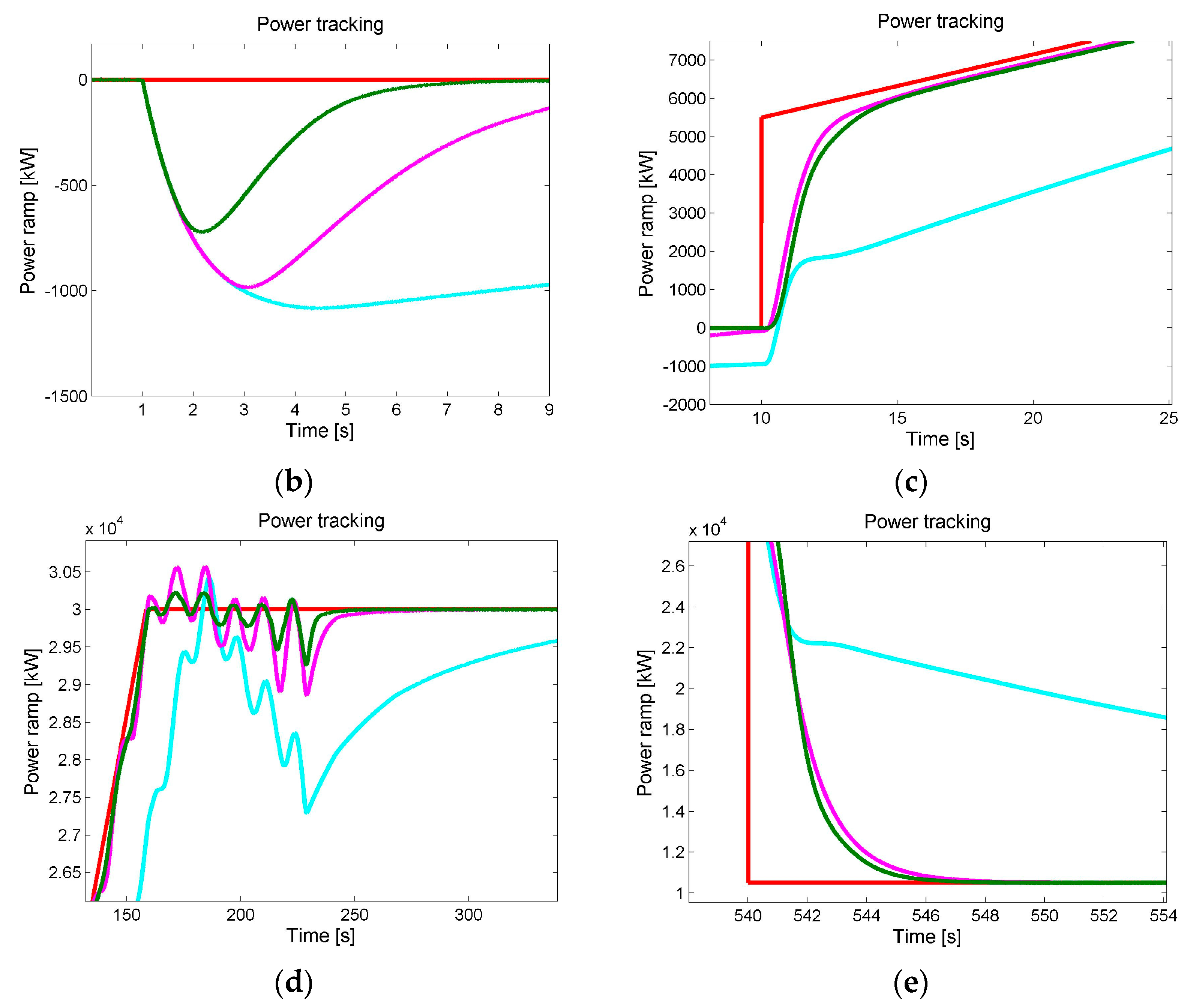
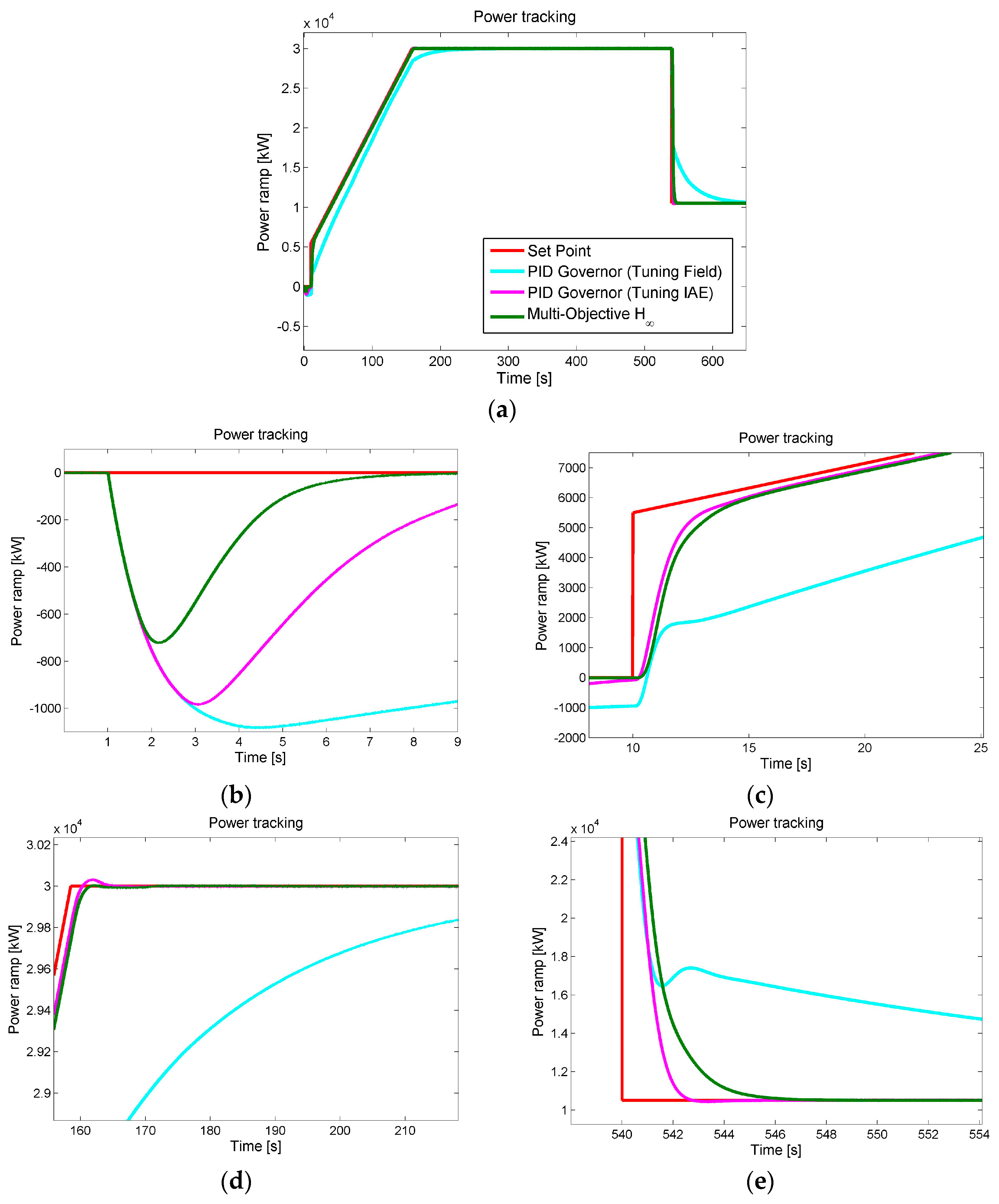
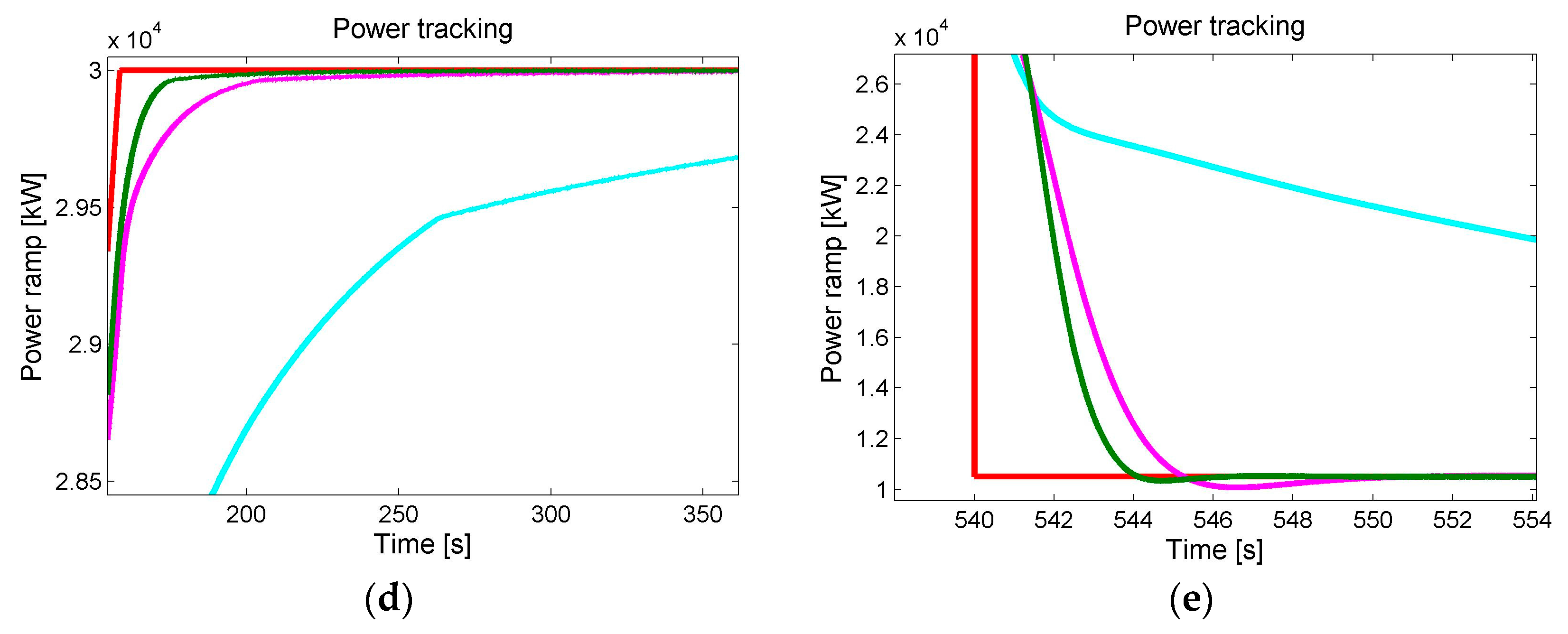
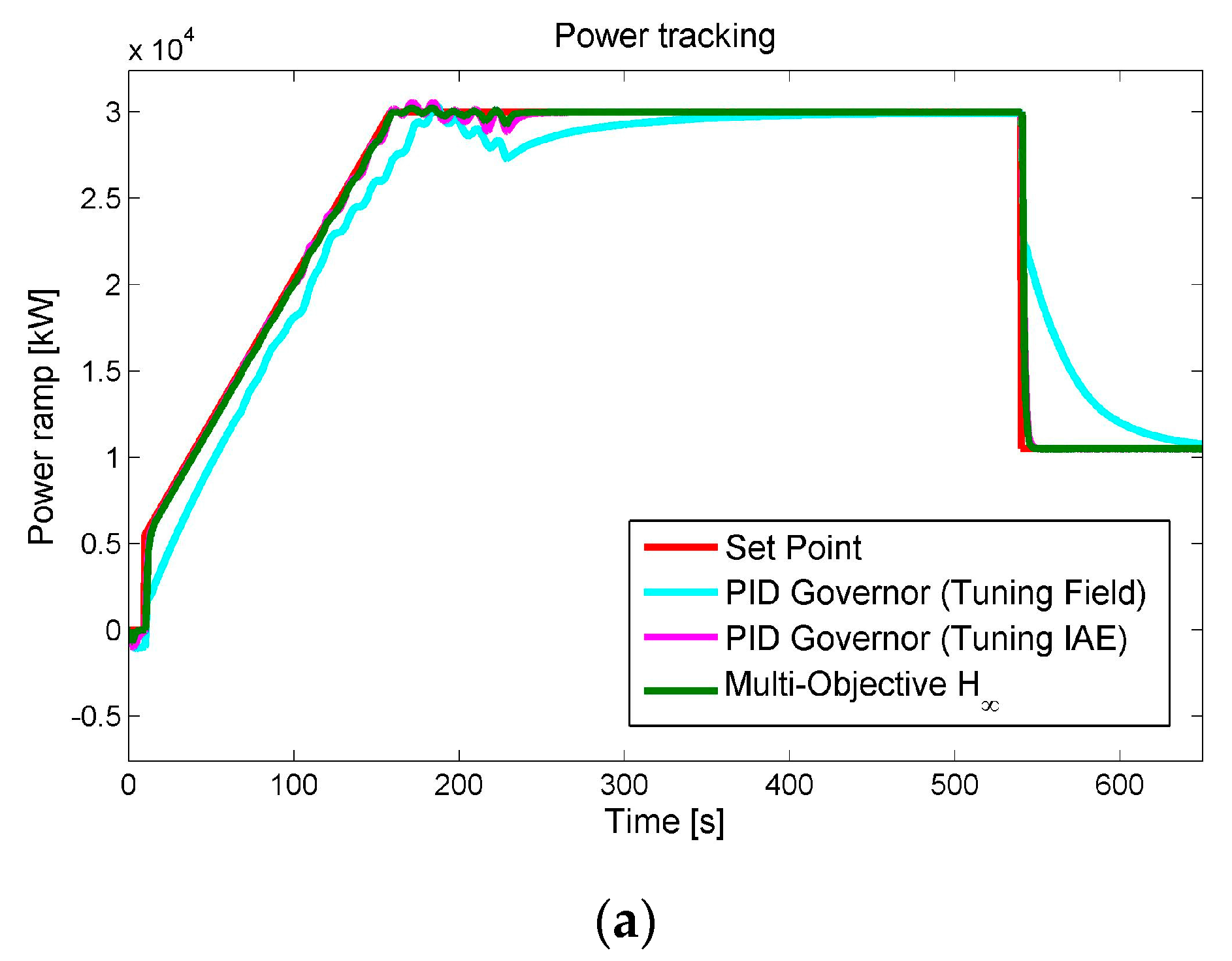
The power tracking of the nonlinear system with the two controllers is depicted in Figure 21. If the IAE tuning set is considered, the two controllers fulfill good reference tracking, whereas for disturbances rejection the robust control technique is faster than the PID. When the PID Governor holds the original gains values set on the site, the control action is very slow and consequently the disturbance rejection and the reference tracking is detuned. The multi-objective robust controller in this case allows improving the performance of 5.8% about the settling time, 6.2% about the rise time and 94% about the IAE index. The set-point following performance indexes are synthetized in Table 3.
4.2. Perturbed Conditions with Typical Loading Ramp
Figure 22 shows the simulation results of the power tracking. If the IAE tuning set is considered, despite the additional power losses and the changing conditions of the steam, the set-point tracking of the two controllers is good. The proposed method allows quickly rejecting the disturbance in the initial stage of the power ramp and is faster than the PID Governor, as shown in Table 4. The performance indexes like settling time and rise time are slightly changed from the nominal case, although the perturbed conditions, only the IAE index is worse but the performances are still satisfactory. When the PID Governor holds the original gains value set on the site, is unable to deal with the parametric variations affecting the system, as is clearly shown in Figure 22. The slow control action does not allow to timely follow the reference. The multi-objective robust controller in this case shows the best behavior: it improves the performance of 21.2% about the settling time, 5.7% about the rise time and 94.9% about the IAE index.
4.3. Perturbed Conditions with an Unexpected Variation of the Steam
The power tracking of the nonlinear system with the two controllers is depicted in Figure 23. If the IAE tuning set is considered, the two controllers fulfill good reference tracking and disturbances rejection but as the perturbations gradually increase, the performances of the PID Governor decrease as it shown from the performance indexes of these last two experiments. When the PID Governor holds the original gains values, the slow control action leads to poor tracking of the power reference, difficulties in managing the perturbed profile of the steam and consequently worse performances with respect to the perturbed conditions of the second experiment. The multi-objective robust controller does not suffer substantial degradation of performances and remains the best controller. It improves the performance of 41.7% about the settling time, 11.1% about the rise time and 94.2% about the IAE index. The set-point following performance indexes are synthetized in Table 5.
5. Conclusions
The multi-objective robust controller was applied to the power control of a CSP plant composed by two turbines, a gear and a generator. Firstly, the controller was synthetized on the linear model of the system and its performance and robustness were analyzed. The designed controller is of order 35, which makes the implementation of the controller complex. Hence, the controller order was reduced to 4th order through the Balanced Truncation method, allowing an easy implementation on PLC machine. Hereafter a discrete-time controller was obtained and tested on the nonlinear system.
The multi-objective robust controller was compared to the current PID-based governing system with two type of setup gains. The IAE optimization method was considered here for the PID Governor tuning, although this technique is not used on site and a more conservative although less performing tuning procedure is adopted. Three experiments were performed for each tuning set: a test with unperturbed conditions, and two tests with perturbed conditions. The proposed controller effectively deals with the dynamic parametric variations of the system, showing its robustness, reporting a fast rejection of the disturbances, ensuring better performance compared of the PID Governor, which is ineffective and cannot guarantee the same performance of an advance control technique without complex automated and self-tuning on-line procedures.
Future work will deal with experiments on the use of GA, or Fuzzy Multi-Objective Linear Programming (FMOLP) techniques [36] that can be applied in different contexts and to solve problems with fuzzy constraints, such as, for instance, in the application that has been recently presented in [37]. These strategies will allow supporting the design procedure, which is often complex, as it requires experience and the accomplishment of a time-consuming series of steps before getting the required performance objectives. Currently, GA-based techniques are being investigated, to the aim of finding the optimal parameters of the weighting functions with a given structure by maximizing a fitness function that is related to the performance of the control.
Author Contributions
This paper is part of the Master Thesis of Vincenzo Iannino, who has therefore carried out most of the work presented here. Valentina Colla and Mario Innocenti were the supervisors of this work, provided indications and guidelines and reviewed all the steps of the work, whereas Annamaria Signorini was the technical manager of the industrial partner and supported the evaluation of the achieved results.
Conflicts of Interest
The authors declare no conflict of interest.
Abbreviations
| AI | Artificial Intelligence |
| ANFIS | Adaptive Neuro Fuzzy Inference System |
| CPC | Current to Pressure Converter |
| CRHPC | Constraint Receding Horizon Predictive Control |
| CSP | Concentrated Solar Power |
| GA | Genetic Algorithms |
| GPC | General Predictive Control |
| HDAC | Hydraulic Double Acting Cylinder |
| HP | High Pressure |
| HPC | Hydraulic Pilot Cylinder |
| IAE | Integral Absolute Error |
| IMC | Internal Model Control |
| LLFT | Lower Linear Fractional Transformation |
| LMI | Linear Matrix Inequalities |
| LP | Low Pressure |
| LQR | Linear Quadratic Regulator |
| MBC | Model Based Control |
| MIMO | Multiple Input Multiple Output |
| MISO | Multiple Input Single Output |
| MPC | Model Predictive Control |
| MRAC | Model Reference Adaptive Controller |
| PI | Proportional Integral |
| PID | Proportional Integral Derivative |
| PLC | Programmable Logic Controller |
| PSO | Particle Swarm Optimization |
| PV | Photovoltaics |
| RBFNN | Radial Basis Function Neural Networks |
| ULFT | Upper Linear Fractional Transformation |
Symbols
| Steam gain | |
| Rated power | |
| Inlet steam mass flow | |
| Maximum steam mass flow | |
| Actual steam conditions | |
| Rotational speed | |
| Synchronism rotational speed | |
| Turbine mechanical drive power | |
| Turbine useful power output | |
| Turbine friction power losses | |
| Bearing power losses | |
| HP turbine torque | |
| LP turbine torque | |
| Gearbox friction torque | |
| Electric generator torque | |
| Windage and bearing friction torque | |
| Full load torque power losses | |
| Total moment of inertia | |
| HP turbine moment of inertia | |
| LP turbine moment of inertia | |
| Gearbox moment of inertia | |
| Generator moment of inertia | |
| Full load power losses | |
| Windage and bearing rated power losses | |
| Electric power | |
| Gearbox power losses | |
| Electric generator power losses | |
| Complex Laplace variable | |
| Extended plant transfer matrix | |
| Nominal plant transfer matrix | |
| Controller transfer matrix | |
| Transfer matrix from to | |
| Generalized disturbance | |
| Controlled variable | |
| Measurement output | |
| Control input | |
| LLFT | |
| ULFT | |
| -norm | |
| Largest singular value of | |
| cost function | |
| Sensitivity | |
| Complementary sensitivity | |
| Control effort | |
| Weigh function | |
| Actuator transfer function | |
| Look-up table gain | |
| Unknown uncertainty | |
| Real uncertainty parameter | |
| Magnitude of | |
| Absolute value of | |
| Turbine transfer matrix | |
| Sensor transfer matrix | |
| Sensor time constant | |
| Reference input | |
| Disturbance input | |
| Noise input | |
| Uncertainty output | |
| Uncertainty input | |
| Tracking error | |
| Structured Singular Value | |
| Transfer matrix from to | |
| Transfer matrix from to |
References
- Webber, M. Catch-22: Water vs. Energy. Sci. Am. 2008, 18, 34–41. [Google Scholar] [CrossRef]
- Camacho, E.; Samad, T.; García-Sanz, M.; Hiskens, I. Control for Renewable Energy and Smart Grids. Available online: http://www.ieeecss.org/general/impact-control-technology (accessed on 16 July 2017).
- Viebahn, P.; Lechon, Y.; Trieb, F. The potential role of concentrated solar power (CSP) in Africa and Europe—A dynamic assessment of technology development, cost development and life cycle inventories until 2050. Energy Policy 2011, 39, 4420–4430. [Google Scholar] [CrossRef]
- Barlev, D.; Vidu, R.; Stroeve, P. Innovation in concentrated solar power. Sol. Energy Mater. Sol. Cells 2011, 95, 2703–2725. [Google Scholar] [CrossRef]
- Zhang, H.; Baeyens, J.; Degrève, J.; Cacères, G. Concentrated solar power plants: Review and design methodology. Renew. Sustain. Energy Rev. 2013, 22, 466–481. [Google Scholar] [CrossRef]
- Ang, K.H.; Chong, G.; Li, Y. PID Control System Analysis, Design, and Technology. IEEE Trans. Control Syst. Technol. 2005, 13, 559–579. [Google Scholar]
- Toodeshki, M.; Askari, J. Model-Reference Adaptive Control for a nonlinear boiler-turbine system. In Proceedings of the IEEE International Conference on Industrial Technology, Chengdu, China, 21–24 April 2008; pp. 1–6. [Google Scholar]
- Wen-Lei, L. Nonlinear uncertain turbine governor design based on adaptive backstepping method. In Proceedings of the 31st Chinese Control Conference (CCC), Hefei, China, 25–27 July 2012; pp. 744–749. [Google Scholar]
- Diaz de Corcuera, A.; Pujana-Arrese, A.; Ezquerra, J.M.; Segurola, E.; Landaluze, J. H∞ based control for load mitigation in wind turbines. Energies 2012, 5, 938–967. [Google Scholar] [CrossRef]
- Nademi, H.; Tahami, F. Robust controller design for governing steam turbine power generators. In Proceedings of the 12th International Conference on Electrical Machines and Systems (ICEMS), Tokyo, Japan, 15–18 November 2009. [Google Scholar]
- Moradi, H.; Bakhtiari-Nejad, F.; Saffar-Avval, M. Robust control of an industrial boiler system; a comparison between two approaches: Sliding mode control & H∞ technique. Energy Convers. Manag. 2009, 50, 1401–1410. [Google Scholar]
- Wu, J.; Nguang, S.K.; Shen, J.; Liu, G.; Li, Y.G. Robust H∞ tracking control of boiler-turbine systems. ISA Trans. 2010, 49, 369–375. [Google Scholar] [CrossRef] [PubMed]
- Mier, D.; Môllenbruck, F.; Jost, M.; Grote, W.; Mônnigmann, M. Model predictive control of the steam cycle in a solar power plant. IFAC-PapersOnLine 2015, 48, 710–715. [Google Scholar] [CrossRef]
- Kordestani, M.; Khoshro, M.; Mirzaee, A. Predictive control of large steam turbines. In Proceedings of the 9th Asian Control Conference (ASCC), Istanbul, Turkey, 23–26 June 2013. [Google Scholar]
- Guihua, H.; Lihua, C.; Junpeng, S.; Zhibin, S. Study of Fuzzy PID Controller for Industrial Steam Turbine Governing System. In Proceedings of the International Symposium of Communications and Information Technology (ISCIT), Beijing, China, 12–14 October 2005; pp. 1275–1279. [Google Scholar]
- Kocaarslan, I.; Cam, E.; Tiryaki, H. A fuzzy logic controller application for thermal power plants. Energy Convers. Manag. 2006, 47, 442–458. [Google Scholar] [CrossRef]
- Chaibakhsh, A.; Ghaffari, A. A Model-based coordinated control concept for steam turbine power plants. J. Eng. 2013, 2013, 1–11. [Google Scholar] [CrossRef]
- Ismail, M. Adaptation of PID controller using AI technique for speed control of isolated steam turbine. In Proceedings of the Japan-Egypt Conference on Electronics, Communications and Computers, Alexandria, Egypt, 6–9 March 2012; pp. 85–90. [Google Scholar]
- Kim, Y.-S.; Chung, I.-Y.; Moon, S.-I. Tuning of the PI Controller Parameters of a PMSG Wind Turbine to Improve Control Performance under Various Wind Speeds. Energies 2015, 8, 1406–1425. [Google Scholar] [CrossRef]
- Perng, J.-W.; Chen, G.-Y.; Hsieh, S.-C. Optimal PID Controller Design Based on PSO-RBFNN for Wind Turbine Systems. Energies 2014, 7, 191–209. [Google Scholar] [CrossRef]
- Li, N.; Lv, L. Parameter optimization for turbine DEH control system based on Improved Genetic Algorithm. In Proceedings of the Chinese Control and Decision Conference, Xuzhou, China, 26–28 May 2010; pp. 3326–3328. [Google Scholar]
- Bolek, W.; Sasiadek, J.; Wisniewski, T. Two-valve control of a large steam turbine. Control Eng. Pract. 2002, 10, 365–377. [Google Scholar] [CrossRef]
- Wang, D.; Wang, Z.; Meng, L.; Han, P. Multi-model based IMC design for steam temperature system of thermal power plant. In Proceedings of the International Conference on Test and Measurement (ICTM), Hong Kong, China, 5–6 December 2009; pp. 5–9. [Google Scholar]
- Dettori, S.; Iannino, V.; Colla, V.; Signorini, A. A fuzzy-logic based tuning approaches of PID control for steam turbines for solar applications. Energy Procedia 2017, 105, 480–485. [Google Scholar] [CrossRef]
- Gu, D.-W.; Petkov, P.; Konstantinov, M.M. Robust Control Design with MATLAB®, 2nd ed.; Springer: Heidelberg, Germany, 2005. [Google Scholar]
- Skogestad, S.; Postlethwaite, I. Multivariable Feedback Control, 2nd ed.; Wiley: New York, NY, USA, 2005. [Google Scholar]
- Zhou, K.; Doyle, J.; Glover, K. Robust and Optimal Control, 1st ed.; Prentice Hall: Upper Saddle River, NJ, USA, 1995. [Google Scholar]
- Pourbeik, P. Dynamic models for turbine-governors in power system studies. In IEEE Task Force Report on Turbine Governor Modeling; IEEE Power & Energy Society: Piscataway, NJ, USA, 2013. [Google Scholar]
- Chaibakhsh, A.; Ghaffari, A. Steam turbine model. Simul. Model. Pract. Theory 2008, 16, 1145–1162. [Google Scholar] [CrossRef]
- Dettori, S.; Colla, V.; Salerno, G.; Signorini, A. Steam Turbine models for monitoring purposes. Energy Procedia 2017, 105, 524–529. [Google Scholar] [CrossRef]
- Doyle, J.; Glover, K.; Khargonekar, P.; Francis, B. State-space solutions to standard H2 and H∞ control problems. IEEE Trans. Autom. Control 1989, 34, 831–847. [Google Scholar] [CrossRef]
- Gahinet, P.; Apkarian, P. A linear matrix inequality approach to H∞ control. Int. J. Robust Nonlinear Control 1994, 4, 421–448. [Google Scholar] [CrossRef]
- Iwasaki, T.; Skelton, R. All controllers for the general H∞ control problem: LMI existence conditions and state space formulas. Automatica 1994, 30, 1307–1317. [Google Scholar] [CrossRef]
- Lavretski, E.; Wise, K.A. Robust and Adaptive Control; Springer: Berlin, Germany, 2013. [Google Scholar]
- Åström, K.; Hägglund, T. PID Controllers: Theory Design and Tuning, 2nd ed.; International Society of Automation (ISA): Research Triangle Park, NC, USA, 1995. [Google Scholar]
- Zimmermann, H.-J. Fuzzy programming and linear programming with several objective functions. Fuzzy Sets Syst. 1978, 1, 45–55. [Google Scholar] [CrossRef]
- Sisca, F.G.; Fiasché, M.; Taisch, M. A Novel hybrid modelling for aggregate production planning in a reconfigurable assembly unit for optoelectronics. In ICONIP 2015 Proceeings, Part II, Proceedings of the 22nd International Conference on Neural Information Processing, Istanbul, Turkey, 9–12 November 2015; Springer-Verlag New York, Inc.: New York, NY, USA, 2015; Volume 9490, pp. 571–582. [Google Scholar]
Figure 1.
CSP plant schematic diagram considered in the present work.

Figure 2.
Block-diagram of the power control in the CSP plant.

Figure 3.
Simplified Simulink model of a turbine.

Figure 4.
Detailed Simulink model of the electro-hydraulic system.
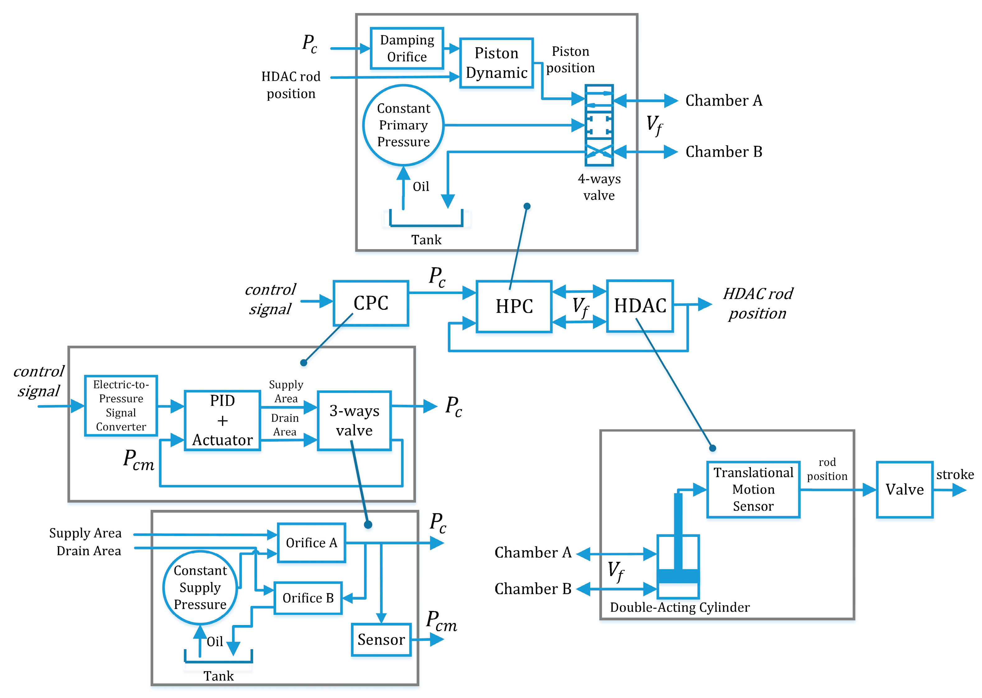
Figure 5.
General closed-loop interconnection.

Figure 6.
Mixed sensitivity optimization scheme.
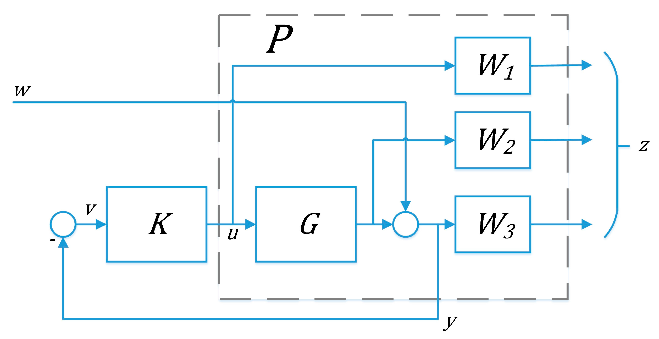
Figure 7.
Singular value frequency response performance requirements for sensitivity and complementary sensitivity functions (taken from [34] with permission).
Figure 7.
Singular value frequency response performance requirements for sensitivity and complementary sensitivity functions (taken from [34] with permission).

Figure 8.
Signal-based control problem.

Figure 9.
Block-diagram of the power control in the CSP plant linear model.
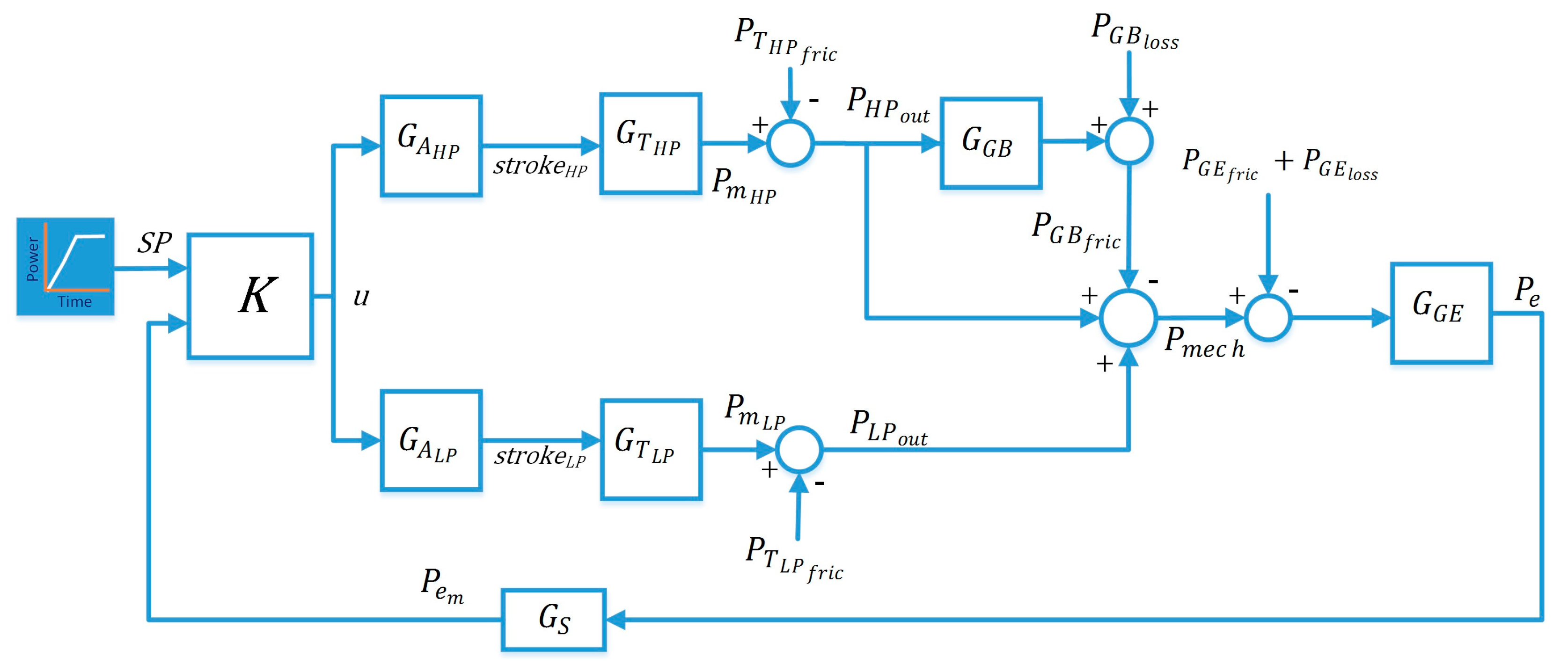
Figure 10.
Actuator with input multiplicative uncertainty.

Figure 11.
(a) Turbine model with uncertainty parameter pulled out; (b) Sensor model with uncertainty parameter pulled out.
Figure 11.
(a) Turbine model with uncertainty parameter pulled out; (b) Sensor model with uncertainty parameter pulled out.
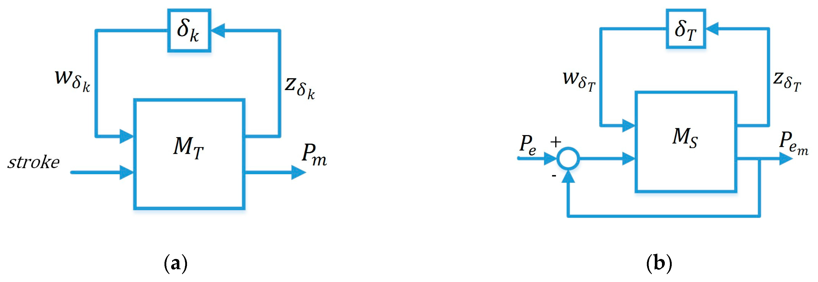
Figure 12.
Block diagram of the closed-loop system with uncertainties and performance specifications.
Figure 12.
Block diagram of the closed-loop system with uncertainties and performance specifications.

Figure 13.
Power ramp reference.

Figure 14.
-iteration computed through the command “hinfsyn”.
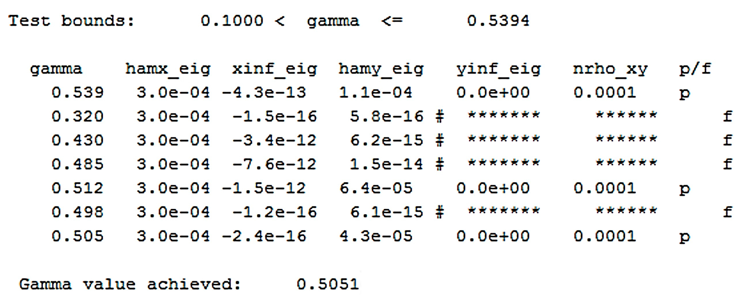
Figure 15.
Closed-loop power reference tracking of the nominal system: (a) Complete view; (b) Disturbance rejection in the initial stage; (c) Ramp command start ; (d) Steady-state at 30 MW; (e) Power profile in the final stage.
Figure 15.
Closed-loop power reference tracking of the nominal system: (a) Complete view; (b) Disturbance rejection in the initial stage; (c) Ramp command start ; (d) Steady-state at 30 MW; (e) Power profile in the final stage.

Figure 16.
Nominal performance objectives: (a) Ideal model matching error; (b) control action; (c) stroke valves.
Figure 16.
Nominal performance objectives: (a) Ideal model matching error; (b) control action; (c) stroke valves.

Figure 17.
(a) Upper and lower bound of ; (b) Upper and lower bound of .

Figure 18.
Closed-loop power reference tracking with random samples of the uncertain system: (a) Complete view; (b) Disturbance rejection in the initial stage; (c) Ramp command start; (d) Steady-state at 30 MW; (e) Power profile in the final stage.
Figure 18.
Closed-loop power reference tracking with random samples of the uncertain system: (a) Complete view; (b) Disturbance rejection in the initial stage; (c) Ramp command start; (d) Steady-state at 30 MW; (e) Power profile in the final stage.

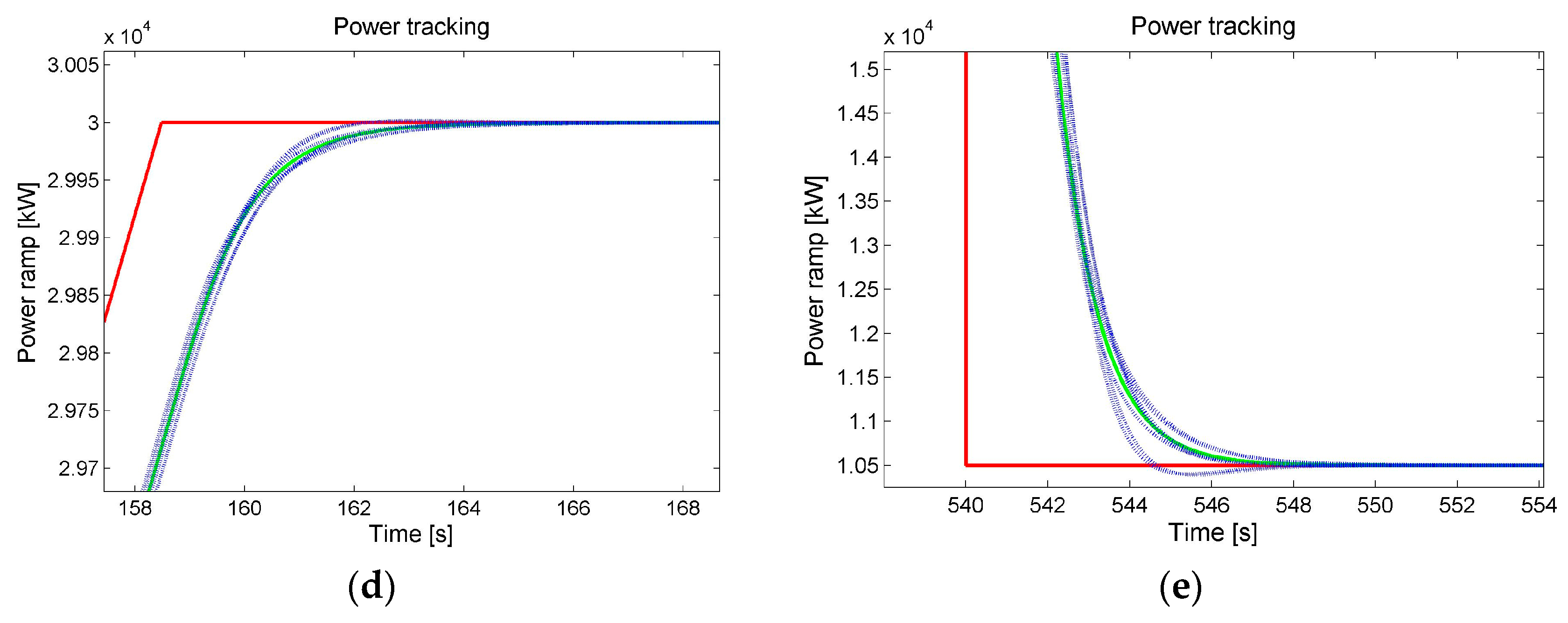
Figure 19.
Frequency response of full order controller and reduced order controller.

Figure 20.
Unexpected steam conditions profile.
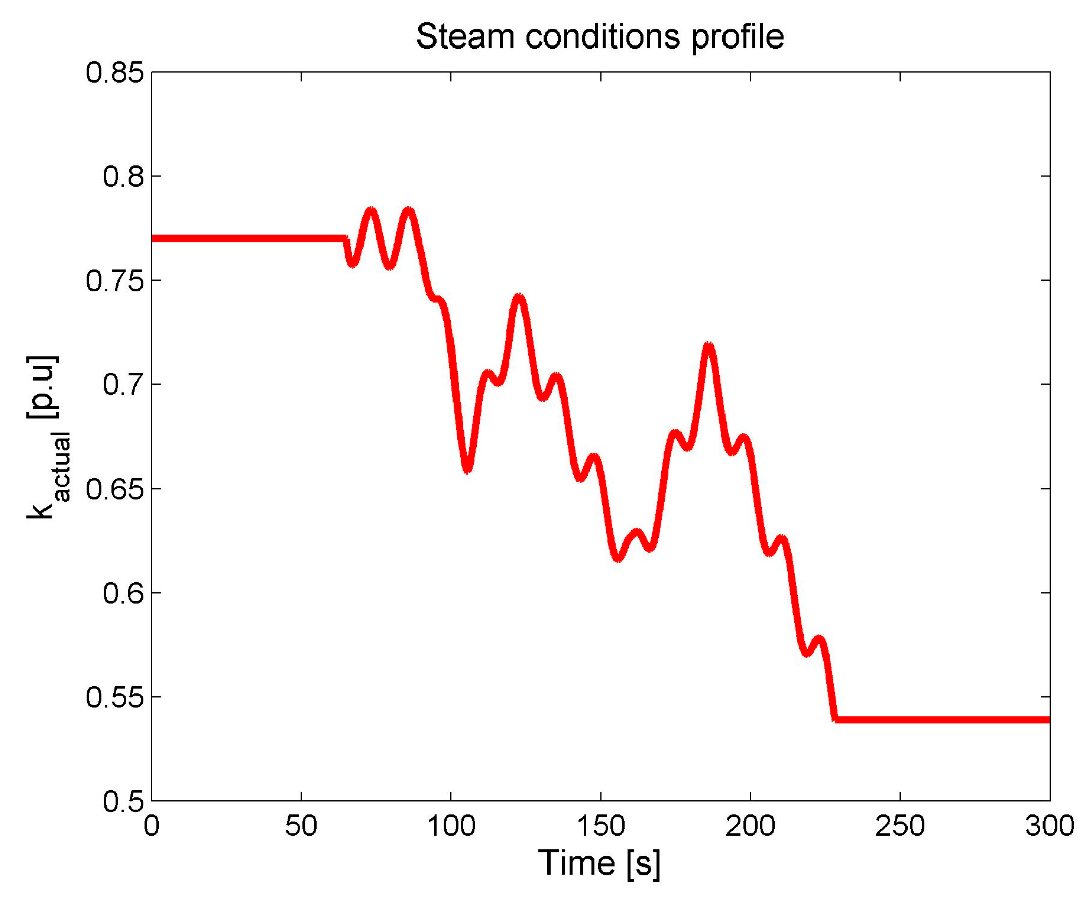
Figure 21.
Closed-loop power reference tracking of the nonlinear system. Comparison between the multi-objective robust controller and the PID Governor tuned with IAE settings and site settings: (a) Complete view; (b) Disturbance rejection in the initial stage; (c) Ramp command start; (d) Steady-state at 30 MW; (e) Power profile in the final stage.

Figure 22.
Closed-loop power reference tracking of the perturbed nonlinear system. Comparison between the multi-objective robust controller and the PID Governor tuned with IAE settings and site settings: (a) Complete view; (b) Disturbance rejection in the initial stage; (c) Ramp command start; (d) Steady-state at 30 MW; (e) Power profile in the final stage.
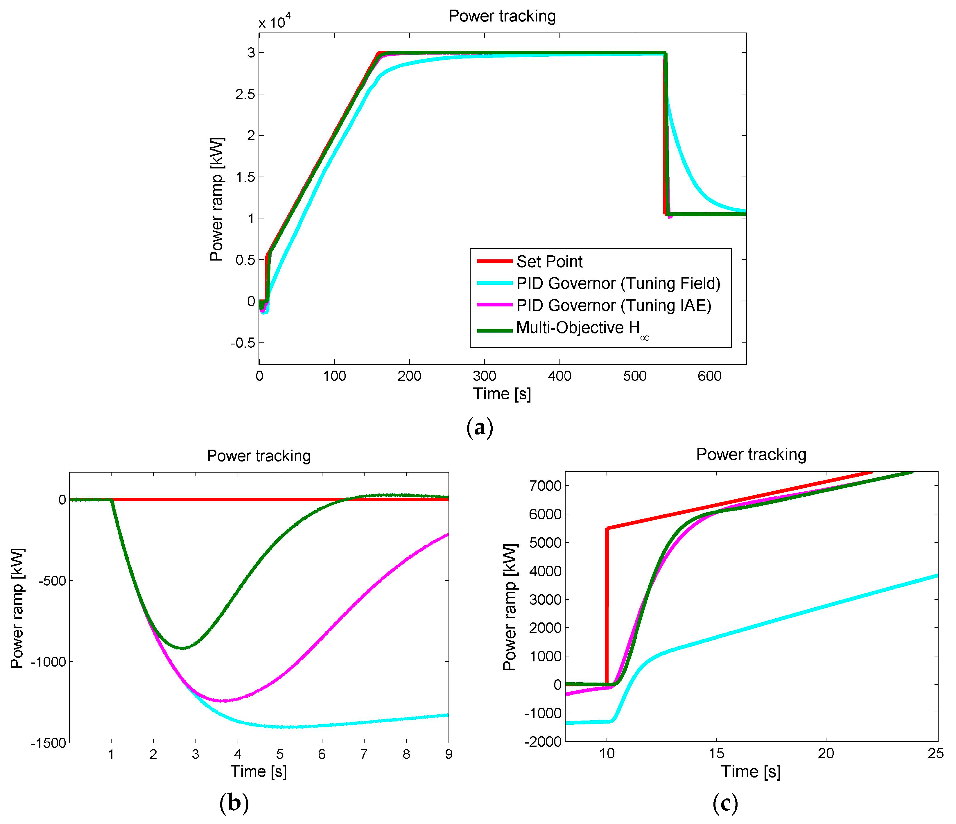

Figure 23.
Closed-loop power reference tracking of the perturbed nonlinear system. Comparison between the multi-objective robust controller and the PID Governor tuned with IAE settings and site settings: (a) Complete view; (b) Disturbance rejection in the initial stage; (c) Ramp command start; (d) Steady-state at 30 MW; (e) Power profile in the final stage.


Table 1.
controller set-point performance indexes.
| Index | Value |
|---|---|
| Settling time (s) | 140.1 |
| Rise time (s) | 130.3 |
| Overshoot (%) | 0 |
| IAE | 3.5933104 |
Table 2.
full order and reduced order controller set-point performance indexes.
| Order | Settling Time (s) | Rise Time (s) | Overshoot (%) | IAE |
|---|---|---|---|---|
| 4 | 140.2 | 130.4 | 0 | 3.8819104 |
| 35 | 140.1 | 130.3 | 0 | 3.6436104 |
Table 3.
Comparison between the set-point performance indexes of the different controllers.
| Controller | Settling Time (s) | Rise Time (s) | Overshoot (%) | IAE |
|---|---|---|---|---|
| PID Governor (Tuning Field) | 148.5 | 138.7 | 0 | 5.3188105 |
| PID Governor (Tuning IAE) | 139.4 | 129.9 | 0.15 | 2.3570104 |
| Multi-Objective | 139.9 | 130.2 | 0 | 3.1240104 |
Table 4.
Comparison between the set-point performance indexes of the different controllers.
| Controller | Settling Time (s) | Rise Time (s) | Overshoot (%) | IAE |
|---|---|---|---|---|
| PID Governor (Tuning Field) | 179.4 | 137.9 | 0 | 1.0283106 |
| PID Governor (Tuning IAE) | 141.7 | 130.7 | 0 | 6.1366104 |
| Multi-Objective | 140.7 | 130 | 0 | 5.1867104 |
Table 5.
Comparison between the set-point performance indexes of the different controllers.
| Controller | Settling Time (s) | Rise Time (s) | Overshoot (%) | IAE |
|---|---|---|---|---|
| PID Governor (Tuning Field) | 243.1 | 147.2 | 1.64 | 9.3471105 |
| PID Governor (Tuning IAE) | 143.1 | 131.9 | 2.1 | 7.7127104 |
| Multi-Objective | 141.7 | 130.9 | 0.9 | 5.4491104 |
© 2017 by the authors. Licensee MDPI, Basel, Switzerland. This article is an open access article distributed under the terms and conditions of the Creative Commons Attribution (CC BY) license (http://creativecommons.org/licenses/by/4.0/).
Share and Cite
MDPI and ACS Style
Iannino, V.; Colla, V.; Innocenti, M.; Signorini, A. Design of a H∞ Robust Controller with μ-Analysis for Steam Turbine Power Generation Applications. Energies 2017, 10, 1026. https://doi.org/10.3390/en10071026
AMA Style
Iannino V, Colla V, Innocenti M, Signorini A. Design of a H∞ Robust Controller with μ-Analysis for Steam Turbine Power Generation Applications. Energies. 2017; 10(7):1026. https://doi.org/10.3390/en10071026
Chicago/Turabian StyleIannino, Vincenzo, Valentina Colla, Mario Innocenti, and Annamaria Signorini. 2017. "Design of a H∞ Robust Controller with μ-Analysis for Steam Turbine Power Generation Applications" Energies 10, no. 7: 1026. https://doi.org/10.3390/en10071026
Note that from the first issue of 2016, this journal uses article numbers instead of page numbers. See further details here.