An Optimization Framework for Investment Evaluation of Complex Renewable Energy Systems

1
DSc Program on Complex Engineering Systems, Universidad de Talca, Curicó 3341717, Chile;
2
Department of Industrial Engineering, Universidad de Talca, Curicó 3341717, Chile
3
Department of Industrial Technologies, Universidad de Talca, Curicó 3341717, Chile
*
Author to whom correspondence should be addressed.
Energies 2017, 10(7), 1062; https://doi.org/10.3390/en10071062
Submission received: 31 May 2017
/
Revised: 10 July 2017
/
Accepted: 11 July 2017
/
Published: 22 July 2017
(This article belongs to the Special Issue Energy Production Systems)
Abstract
:Enhancing the role of renewable energies in existing power systems is one of the most crucial challenges that society faces today. However, the high variability of their generation potential and the temporal disparity between the demand and the generation potential represent technological and operational gaps that burden the massive incorporation of renewable sources into power systems. Energy storage technologies are an alternative to tackle this gap; nonetheless, their incorporation within large-scale power grids calls for decision-making tools that ensure an appropriate design and sizing of power systems that exploit the benefits of incorporating storage facilities along with renewable generation power. In this paper, we present an optimization framework for aiding the evaluation of the strategic design of complex renewable power systems. The developed tool relies on an optimization problem, the generation, transmission, storage energy location and sizing problem, which allows one to compute economically-attractive investment plans given by the location and sizing of generation and storage energy systems, along with the corresponding layout of transmission lines. Results on a real case study (located in the central region of Chile), characterized by carefully-curated data, show the potential of the developed tool for aiding long-term investment planning.
1. Introduction and Motivation
One of the main challenges of today’s society corresponds to evolving the energy generation matrix due to economical and environmental arguments. According to [1], 81.4% of the world’s primary energy comes from fossil fuels, which exposes us to high economic and environmental risks; on the one hand, current forecasts indicate that fossil fuel reserves might reach critical levels in 2050–2100 [2,3,4], and on the other, fossil fuels are responsible for most of greenhouse gas emissions. The penetration of generation technologies based on renewable sources, such as solar and wind power, seems as the only sustainable alternative for a world with a constant increase of energy demand; see, e.g., [1]. One of the main technological gaps associated with these energy sources is the high variability of their generation potential and the temporal disparity between the demand and the generated energy. These two issues can be addressed through energy storage systems (ESSs); however, these are quite costly solutions and respond to quite strict operative patterns. Therefore, their incorporation within large-scale power grids is not only associated with technological challenges, but also calls for decision-making tools that ensure an appropriate design and sizing of power systems that exploit the benefits of incorporating ESSs along with renewable generation power.
Different efforts have been devoted to the development of decision-making tools for strategic power system design. These approaches address different long-term decisions such as the location and capacity of generators and substations, the layout of transmission lines and the incorporation of ESSs. As we will show in the literature review in Section 2, these tools do not incorporate all decision dimensions simultaneously, and they are typically devised from the perspective of the system operator. On the one hand, this implies that they do not take into account the fact that power grid components work collectively and simultaneously; and on the other, they dismiss the fact that in the current energy market conditions, design tools must respond to the financial expectations of investors. Hence, we believe that there is a need for designing an investor-oriented decision-making framework that incorporates generation, transmission and storage decisions; such a tool aims at exploiting the competitiveness, the attractiveness and the profitability of new renewable energy-based systems.
Contribution and Paper Outline
The main contribution of our paper is an optimization modeling framework, based on a mixed integer linear programming (MILP) model, for supporting decision-making in (renewable-based) complex energy systems’ planning. By means of a curated case study, we show the potential of the proposed approach in providing economically-attractive investment plans that exploit the use of ESSs. Furthermore, we also investigate the use of the proposed tool for analyzing the impact of technological advances in ESSs.
The paper is organized as follows. A literature review on related applications is presented in Section 2. The optimization model that embodies our modeling framework is presented in Section 3. In Section 4, we present the results obtained when applying the designed optimization model to our case study. Finally, conclusions and paths for future work are drawn in Section 5.
2. Literature Review
As mentioned in the previous section, over the last few years, several efforts have been devoted to providing a modeling and algorithmic framework for aiding strategic decision-making in energy system design; see [5] for a general reference on design by optimization of electrical energy systems. In this section, we review some of the most recent and relevant examples associated with our planning setting. Our review focuses on decision-making tools concerning decisions on: (i) the location and sizing of renewable-based generators; (ii) the layout and sizing of transmission grids; and (iii) the location and sizing of ESSs. After a detailed analysis, we have selected 18 articles, all of them published over the last six years, where optimal energy system planning approaches, concerning these decisions, are investigated. In Table 1, we summarize the characteristics of these articles according to three criteria: storage, generation and transmission. With respect to storage, we differentiate among those papers where capacity is decided (“capacity”), where location is decided (“location”), or where other characteristics (“others”), such as operational profiles (“Op.”) or technological assessment (“Tech.”), are within the decision scope. A similar classification is considered for generation decisions. In the case of transmission decisions, we identify which papers consider layout design (“layout”), which consider decisions on lines’ capacity (“capacity”) and which consider decisions on power flow over the designed or existing lines (“flow”).
As can be seen from the table, some of the existing works mainly focus on the design of optimal storage systems; for instance, the work presented in [11]. In that paper, the authors provide a mathematical optimization model where the solutions correspond to the design of a storage system that defines its storage capacity, its location within the existing power system, its operative regime and how this system will be integrated, through new transmission lines, into the existing grid. On the contrary, other papers, such as [16], do not take into account the implementation of ESSs, and their core corresponds to the design of optimal renewable-based generation strategies (capacity and location), along with the definition of a corresponding grid (layout and capacity). A similar design setting as the one discussed in this paper is approached in [21]; in that work, an optimal investment plan of hybrid renewable generation technologies is studied in the context of microgrids. Similarly, a joint investment and operation framework is studied in [22] for the sizing of solar energy, wind energy and energy storage units using realistic microgrid data. Furthermore, the location and sizing of hybrid renewable generators over multiple locations in distributed microgrid systems is studied in [23]. In addition to these cases, the other articles summarized in Table 1 focus on different aspects of the decision-making setting motivated in the Introduction; nonetheless, none of them offers a general modeling framework integrating all of the decisions in a systematic fashion. Moreover, none of them emphasizes the need for considering the investor perspective as a fundamental characteristic of any real-world-oriented decision-making tool for large power systems. Our work, as can be seen from the last line of the table, offers an integrated decision-making framework that closes this methodological gap. Furthermore, we will show in the following section that our framework aims at designing economically-attractive energy systems by optimizing the economic value of the sought investment strategies.
3. Problem Definition
The core of our energy system planning tool corresponds to an optimization problem, the given MILP problem, that we coined as the Generation, Transmission, Storage Energy Location and Sizing Problem (GTSELSP). The GTSELSP involves technological and economical considerations, and it is associated with a quite complex mathematical formulation, which will be described in this section.
3.1. Problem Notation: Parameters and Variables
3.1.1. Sets
The sets that we use in our problem definition are the following:
- set of candidate locations where generation plants can be located.
- set of candidate locations where substations or line junctures can be located.
- set of selling points, i.e., sub-stations of the existing power grid where energy is associated with a spot price.
- set of potential lines connecting generation locations from with locations in (i.e., ).
- set of lines connecting locations from with both, other elements from and selling points from O (i.e., ).
The designed tool seeks for strategic decisions, which are evaluated through a long-term evaluation of the corresponding operational decisions. The strategic evaluation time span corresponds to years. Each of these years is characterized by a representative year (equal for all years). This representative year is divided into cluster-days that represent shrunk periods (e.g., one month is shrunk into one day); index t will represent one hour of each of these cluster-days. As will be shown in Section 4, the composition of such cluster-days has a strong influence on the computational difficulty of the underlying mathematical optimization model; however, it does not really affect the structure of the corresponding solutions.
3.1.2. Generation Parameters
From a strategic design point of view, please consider the following generation parameters:
- maximum generation capacity to be installed, at a single location (MWp).
- available radiation for a given generation location and a given hour t (MW/m).
- nominal power of a PV module under standard test conditions (STC) (MWp/m) of a photovoltaic (PV) module with a surface of a (m)). Hence, a PV generation plant will be comprised by a group (of say Q) of these modules, and its capacity will be given by (MWp).
- performance of the inverter that is planned to be used in the installed PV plants.
- loss factor of the PV modules due to the presence of dust.
Additionally, from an economic point of view, we use the following parameters:
- fixed cost of installing a PV power plant (USD).
- variable cost of installing a PV power plant (USD/MW).
- variable cost of installing a sub-station (USD/MW).
- variable cost of ESS installation (USD/MWh).
- sale price in node o at period t (USD/MW).
3.1.3. Transmission Parameters
Transmission takes place in lines between generation, transformation (i.e., substation) and the existing grid (where the energy is injected to the system). These lines are characterized by several technological and economic parameters, which are listed below:
- transmission loss factor associated with direct current (DC).
- transmission loss factor associated with alternate current (AC).
- maximum extension of a single line segment due regulations (km).
- distance between point i and point j (km).
- loss factor associated with power transmission.
- fixed installation cost of installing one kilometer of transmission line (USD/km).
- variable installation cost of installing, per MW, one kilometer of transmission line (USD/MW/km).
3.1.4. Energy Storage Parameters
Energy storage systems operate according to the following technological and economical parameters:
- ESS’ charge efficiency.
- ESS’ discharge efficiency.
- minimum level of the state of charge that must be preserved in the ESS.
- maximum ESS’ charge power flow (MW).
- maximum ESS’ discharge power flow (MW).
- maximum storage capacity (MWh).
- variable cost of ESS installation (USD/MWh).
3.1.5. Problem Variables
From a structural point of view, we use the following decision variables:
- binary variable, so that if a generator (i.e., a PV plant) is installed at location , and otherwise.
- installed fraction of of installed generator at a given ().
- installed nominal power (PV) at a given . ().
Operation is characterized by the following decision variables:
- generated power from the generator located at in period t.
- dispatched power from the generator located at in period t.
- spilled power in the generator located at in period t.
- binary variable so that if a substation is installed at location , and otherwise.
- capacity of installed substation, at a given .
The layout of transmission lines is associated with the following decision variables:
- binary variable, so that if a line between i and j is built (), and otherwise.
- binary variable, so that if a line between j and k is built (), and otherwise.
- capacity of installed transmission line, between i and j ().
- capacity of installed transmission line, between j and k is built ().
Furthermore, the operation on transmission lines associated with set is modeled by the decision variables listed below:
- power flow on line in period t.
- non-transmitted power through the line in period t.
- power losses at line in period t.
- power flow on in period t.
- non-transmitted power through the line in period t.
- power losses on in period t.
Additionally, for the location and sizing of the ESS’ facilities, we consider the following variables:
- capacity of the ESS installed at .
- installed portion of of installed ESS at ().
Note that an ESS facility can be installed only on nodes where a generator or a substation is located.
Finally, the operation of the ESS is defined by the following variables:
- charge status, in period t, of the ESS located at i.
- charging flow, in period t, at the ESS located at i.
- discharging flow, in period t, at the ESS located at i.
- binary variable, so that , if the ESS in i is discharged in period t, and , otherwise.
3.2. An MILP for the GTSELSP
Considering the notation presented above, we can now formulate the mixed integer program that encodes the strategic design tool proposed in this paper. The different types of constraints encompassing the GTSELSP are described in the remainder of this subsection.
3.2.1. Generation
The first group of constraints aims at characterizing the total energy produced at the (installed) generators; i.e., generation constraints, and they are given by:
Constraint (1) ensures that generation capacity is installed at given site (; thus ), if and only if it is decided that at such site, a generator is installed (); moreover, the same constraint ensures that the installed capacity will not exceed the predefined maximum capacity . The actual energy flow that leaves a given generation site i at a given time t () is characterized by the constraints in (2); such energy flow depends not only on the installed capacity () the nominal power () or the effect of the dust (), but also on the losses in the line from the panels to the inverter (), the efficiency of the inverter () and the losses from the inverter to the connection point into the grid (). Constraint (3) allows one to split the energy generated at site in time (), into two components; which is the energy that will be injected into the grid, and , which represents the (eventually) spilled energy. Finally, the nature of the involved variables is expressed in (2).
3.2.2. Transmission Topology
The second group of constraints defines the topology and size of the transmission layout, and it is given as follows:
The constraints in (5) ensure that at least one line must by built from the generation site in the case that a power plant is installed at such a site (i.e., if , then ). Additionally, Constraints (6) and (7), ensure the right topology of the connections associated with generation points. The type and topology of the connections from (or towards) installed substations are characterized by Constraints (8) and (9). Constraints (10) and (11) imply that due to technical requirements, the sought layout must be such that no direct connection shall by longer than . The constraints in (12) characterize the nature of the variables.
3.2.3. Energy Storage Systems
The functioning of the (eventually installed) energy storage systems must fulfill several technological rules. Such rules are characterized by the following set of constraints;
An ESS can be installed at a given site (), only if at that site, a generator (, ) or a substation is installed (, ); this requirement is encoded by Constraints (13) and (14), respectively. The constraints in (15) ensure that the nominal installed capacity of an ESS at a given site () is a portion (given by ) of the maximum reference capacity . The amount of energy that can be stored at a given ESS located at , at a period (), cannot exceed its corresponding capacity ; this is enforced by the constraints in (16). Likewise, the minimum energy that shall be kept at the same ESS shall not be less than the state of charge threshold ; this is modeled by the constraints in (17). The constraints in (18) model the fact that the energy stored in the ESS installed at , at a given period , depends on energy stored in the previous period (), the energy that is charged in t () and the energy that is discharged in t (). Complementary to this, the amount of energy that is charged and discharged at a given period t, in an ESS located in , is characterized by Constraints (19) and (20), respectively. Furthermore, the initial conditions of the installed ESS are modeled by the constraints in (21). The nature of the associated variables is characterized by Constraint (22).
3.2.4. Power Balance
So far, we have presented the constraints that define the feasibility conditions of the generation and of the energy storage; however, no linkage among them has been established. This linkage, or coupling, is given by the power balance at each node (generation, storage, and/or substation) and involves the corresponding transmission lines associated with it (and of course, the energy flow through them). The following constraints ensure a correct interdependence among the different energy flows:
The constraints in (23) model the following phenomenon: at a given generation node and in given period , the total energy that leaves i through the corresponding lines () must be equal to the energy that is injected from the corresponding generator (), plus the energy that is discharged from the corresponding ESS (), minus the energy that is charged into the corresponding ESS ().
Similarly, the constraints in (24) ensure a correct energy balance within the intermediate nodes . Basically, these constraints ensure that the total energy that is injected into a given (), plus the energy that is discharged from the ESS located at j (), minus the energy that is charged into the ESS located at j (), must be equal to the energy that leaves j through the associated transmission lines ().
Following (23) and (24), we have that the energy that is injected into a selling point , in , is modeled by . Note that we do not allow generation nor the installation of ESS in the points comprising O.
3.2.5. Transmission and Substation Capacities
The power dispatched from the generation and substation (or line juncture) nodes must respect the capacity of the transmission lines. In the GTSELSP, we not only decide on the layout of the transmission grid, i.e., which lines are constructed, but also the capacity of these lines. The relation among layout, capacity and transmission decisions is encoded by the following constraints;
The constraints in (26) ensure, on the one hand, that the power flow through line , at a given period (), must be less than the installed capacity , and on the other, that we will install such capacity () if an only if a line is built on , i.e., (note that M is a sufficiently large number). The constraints in (27) are equivalent to (26), but on the connections comprising . The nature of the capacity variables is given by (28).
In addition to the transmission lines, the capacity of the installed substations is also part of the decision-making process; the associated constraints correspond to:
The constraints in (29) ensure that the total power that is injected in the substation located at in period () must be less than or equal to the capacity of the substation (); moreover, the same constraints also ensure that if no substation is located at j (), then the corresponding capacity must be zero, as well. Equivalently, the constraints in (30), which are very similar to (29), ensure that the total power dispatched from j, including the corresponding losses (), must also respect the corresponding substation capacity. Finally, Constraint (31) ensures the nature of the substation installation variables.
3.2.6. Losses and Boundary Conditions
As in any real-world-oriented application, we need to take into account the losses in the transmission lines. These losses depend on the power flow and on the efficiency factor, which is inherent to the transmission lines. The constraints:
allow us to express the transmission losses, and , as a portion (given by ) of the power that flows through the lines ( and , respectively).
Along with the constraints presented so far, we also impose boundary conditions that must be preserved: (i) transmission lines cannot be built from a node and towards the same node; (ii) there are no lines outgoing from a selling point (i.e., the grid ends at the selling points); and (iii) we assume that in all selling points , there must be a substation (which switches from the power transmission towards the power distribution). Such conditions are modeled by the following constraints:
3.2.7. The GTSELSP
So far, we have presented all of the constraints that characterize the set of feasible solutions of the GTSELSP. For a full representation of the problem, we shall consider that the objective function corresponds to the maximization of the economical profit of the sought solutions; for a given evaluation time span, such profit is given by the difference between the incomes obtained from selling the produced energy, minus the installation and operation costs. The total income is given by:
and it corresponds to the sum, over the planning horizon, of the gains induced by the power that flows towards the selling points. The total generation installation costs are given by:
Likewise, the total cost of the grid layout construction is given by
as can be seen, the grid installation cost does not only depend on the whether a line is built or not, but also on its capacity. Another crucial investment cost corresponds to the ESS installation, which is given by:
as can be seen, the total cost associated with the ESS infrastructure, mainly depends on the size of the installed units. Finally, the latter installation cost that must be considered corresponds to the substations installation cost, given by:
as well as for the ESS, the substations’ installation cost basically depends on the size of the installed infrastructure. Consequently, we can model the GTSELSP objective (profit) function as:
Note that in this profit formula, we have not included generation costs since they are assumed to be negligible when compared to the installation costs and the total incomes. Since future incomes strongly depend on the future realizations of energy market, we present in Section 4.2 an econometric strategy to address this variability. Please note that in the case that generation costs are relevant, one should adopt complementary strategies as the cost benefits analysis discussed in [24].
Considering all of the elements presented so far, a MILP formulation of the GTSELSP is given by:
This MILP formulation has a polynomial number of variables and constraints; therefore, one could use any of the state-of-the-art solvers, e.g., CPLEX, to tackle it. This enhances the practical use of our approach, since there is no need for developing sophisticated algorithmic strategies to tackle the GTSELSP.
4. Results and Discussion
In this section, we will report results on a case study in which the GTSELSP is used as the core element for the design and evaluation of a large-scale (multi-site) PV-based generation infrastructure. We first contextualize the case study; later, we present an exhaustive analysis of how the problem parameters were estimated; and finally, we present and discuss the obtained results.
4.1. Case Study: Chilean Central Region
Chile has one of the best solar potential in the world; in particular, in the northern region, the average radiation is as high as 2055 (kWh/m) and with a quite stable profile during the day. However, the main sources of energy demand are located in the central region, where the radiation potential fluctuates more. Moreover, the current Chilean power system is comprised by a northern grid and a central grid, which are not connected, making it impossible to exploit the northern solar radiation to satisfy the power demand in the central region. Therefore, a need arises to be able to efficiently exploit the solar potential of the Chilean central region in order to contribute, by a clean and sustainable source, to satisfying the corresponding energy demand.
The following characteristics of the central region play an important role in our decision setting: (i) the average radiation is above 1555 (kWh/m) , which is still higher than the radiation of countries like Germany (1261 (kWh/m)), with high penetration of solar generation; (ii) this area incorporates 51.51% of the Chilean population, implying quite large urban areas, making it impossible to install very large power plants combining substations or ESS facilities; (iii) besides the domiciliary demand, there is also a vast need for electricity for industrial activities such as agriculture, mining and retail; (iv) the orography in this sector is more complex than in the northern region, which incorporates another level of complexity in the design process.
The geographical zone where the solar power generation system is to be designed corresponds to the 6th and 7th regions (see Figure 1a). This zone fulfills two important operative requirements: it is practically attached to the metropolitan area (where most of the demand is concentrated), and there is a quite complex existing power grid infrastructure where our designed power system can eventually be incorporated. In the existing grid, there exists a mix of hydroelectric, diesel and gas power plants, whose generation capacity mainly contributes to satisfying the power demand of the metropolitan area.
In Figure 1b, we display a schematic representation of the geographical data of the considered case study. In the considered zone, we have identified 20 areas where the generation plant could be located; these 20 areas, which comprise set , are represented by yellow circles in Figure 1a,b. The location of potential substations, which yields set , are represented by 15 green squares. The existing substations, where energy is to be injected (i.e., sold) to the power grid, are represented by 11 red squares, comprising set O. Existing, as well as potential transmission lines are not shown for ease of exposition. Besides this topological data, we have curated all other problem parameters; this will be described in detail in the following subsection.
4.2. Estimation and Model Parameters
We have divided the problem parameters into five sets: (i) energy resource parameters, associated with generation zones; (ii) technological parameters, associated with power plants and transmission lines; (iii) generation and transmission construction costs; (iv) energy storage parameters; and (v) spot prices. The process for curating all of these parameters is presented below.
4.2.1. Solar Radiation Potential
The solar radiation potential of the 20 generation zones was calculated using one year of data (with a 30-min resolution) using the tool Explorador Solar. This tool, which was developed by an initiative of the Chilean Ministry of Energy [25], allows on to simulate, using sophisticated meteorological models, daily solar radiation in any location of the Chilean territory for a whole (typical) year.
In Figure 2, we report the radiation potential curve (along the day) of the 20 locations, for four different days; 4 February (summer), 8 May (autumn), 15 August (winter) and 18 November (spring). In these examples, we can see that while the generation potential of the different areas is similar in summer and somewhat in spring, in autumn and, in particular, in winter, this is not the case. This latter situation, which does not occur in northern regions, reinforces the need for an optimized policy design in order to maximize the potential mix along the year.
4.2.2. Generation and Transmission Technological Parameters
To determinate the appropriate instance setup, we needed to find some technological parameters related to power plants and transmission lines.
The necessary parameters related to power plants have been determined using information from Vivest Energías Renovables S.A. (Vivest) [26]. Then, we obtain = 1000 (W/m), = 98%, = 5%, = 97% and = 97%. On the other hand, we also receive the electric transmission loss performance parameter from Vivest. This corresponds to = 1.5% [26].
Furthermore, in our model, we have = 200 (MWp). This parameter comes from the latest renewable energy projects that have been installed and that actually operate in Chile [27]. Finally, = 40 (km), which is the distance threshold defined by the Chilean power operator for ensuring distribution quality of the Chilean grid [28].
4.2.3. Generation and Transmission Construction Costs
The total construction cost associated with PV power plants (measured by U.S. dollars per MW) was curated according to the information provided by [26]. We obtained construction costs associated with different plant sizes, and we used this information to construct, via regression, a linear function associating generation power with construction cost. This is shown in Figure 3; the points in the plot correspond to the information at hand, while the line (along with the information incorporated in the plot) corresponds to the linear regression. As expected, we can see that the construction cost lineally depends () on the generation potential of the PV power plant. Therefore, 1,337,963 (USD) and (USD/MW).
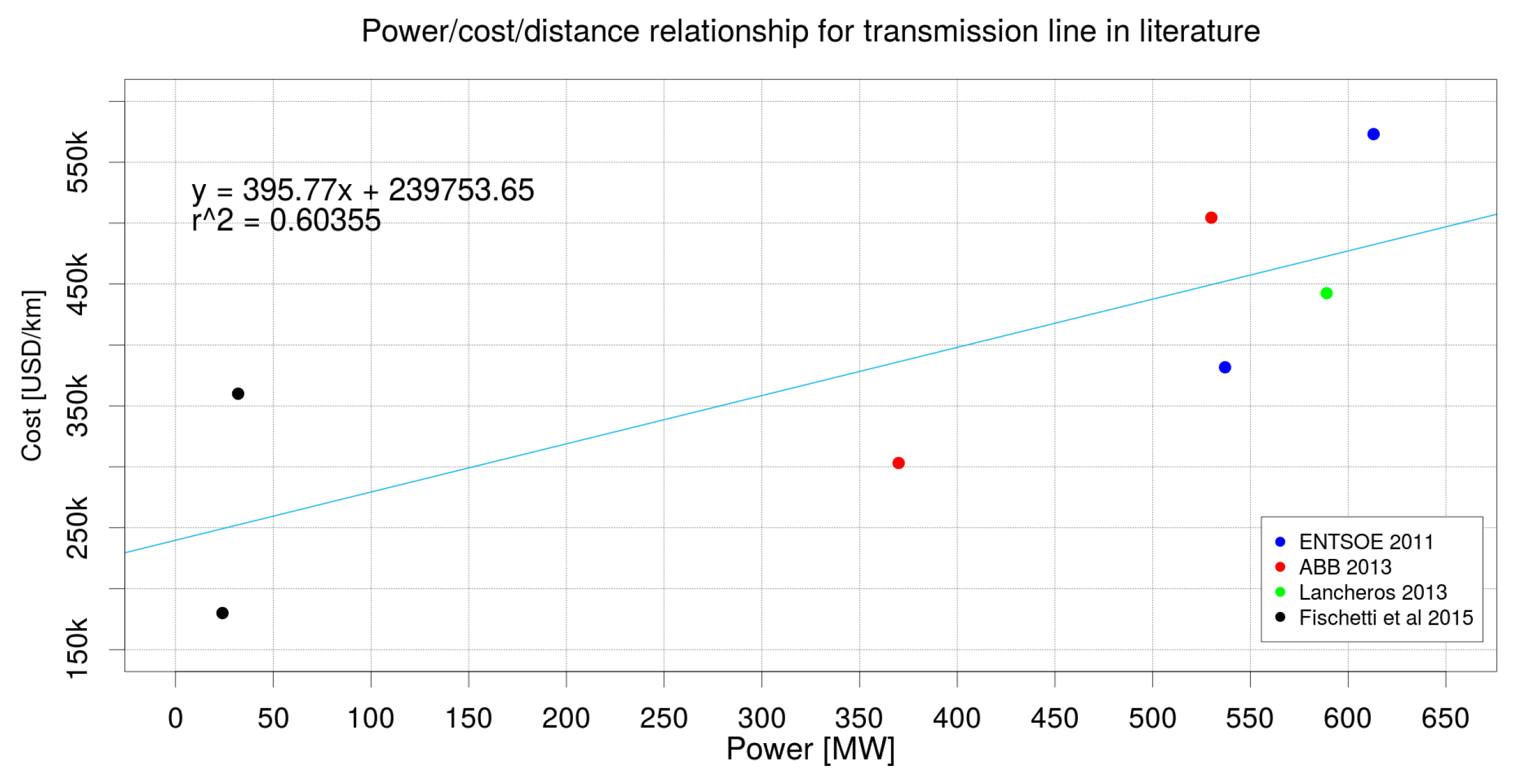
For defining the construction cost of transmission lines, we used the, relatively recent, information published in [29,30,31,32], where the construction cost (in USD per km) associated with seven different lines’ transmission capacity (in MW) is reported. In Figure 4, we display these values by colored points (colors depending on the source). As for the plant construction cost, we also compute a linear regression for approximating both, a fixed and a variable line construction cost. From the obtained regression, we have that (USD/km) and (USD/MW/km). Although the obtained regression is not that accurate (), we believe that it is a quite fair approximation; a better estimation of this cost is out of the scope of this work, and it can be incorporated later on when the tool is used in practice.
The installation cost of substations was approximated by a similar scheme. We considered the installation cost data (in USD/MW) published in [29,30,31,33]. In Figure 5, we display the published construction costs (colored points) and the linear regression associated with these costs. From the obtained regression (), we have that (USD/MW) (fixed installation costs were negligible).
4.2.4. Energy Storage Parameters
As said before, one of the key contributions of our work consists of assessing the economic impact of different ESSs as part of a solar power generation system embedded into a large existing power grid. For such a purpose, we evaluated four storage technologies: the considered technologies are a sodium-nickel chloride cell technology from the so-called Zeolite Battery Research Africa battery protect (ZEBRA), Pb-acid batteries (PBAC), pumped hydroelectric storage (PHS) and compressed air energy storage (CAES). These four technologies are based on different technological principles and, therefore, operate according to different values of their parameters (see Section 3.1). In Table 2, we present the values of the parameters associated with the different technologies and the literature reference from where these values were obtained.
These technologies are in different stages of development. While ZEBRA is a quite new technology, still in the R&D stage, PBAC, PHS and CAES are well-known solutions. Since PHS is the most common technology in our decision-making setting [34], we will consider it as our default technology. Nonetheless, in the following subsection, we will also compare the economic impact of using each of these ESS technologies. As a final remark, in all of our experiments, we assume that the installed ESSs are renewed, within the evaluation horizon (30 years in this case), according to the lifetime reported in Table 2.
4.2.5. Modeling and Estimation of Spot Prices
The energy generated in the different power plants (either the existing or the potential ones) is injected into the grid at the substations. At these substations, the system operator pays for the injected energy at the so-called spot price, which depends on the demand and the generation mix.
For estimating the spot prices in the existing substations, we used historical data from the Economic Dispatch Load Center of the Central Interconnected System (CDEC-SIC) between the years 2015 and 2016 [36]. The resolution of this database is 1 h for each substation. These data were processed by an ad hoc adaptation of a bootstrapping technique [37,38], to produce, for each substation, 1000 possible series (each of them associating one value per hour). Afterwards, these series were used to approximate a so-called empirical density distribution price (EDDP).
In Figure 6 and Figure 7, we show for the Itahue154 and Rapel220 substations, respectively, the EDDPs estimated for four different days in eight different hours. In the presented examples, we can clearly see that the series follow bi-modal distributions; the first mode (associated with lower prices) corresponds to the efficient supply of energy that satisfies most of the demand, while the second mode (associated with higher prices) is likely to be related with contingencies in the power supply or peaks of the demand. The described behavior is quite clear for the case of Itahue154, which represents the spot price behavior of most of the considered substations. As a matter of fact, the different percentiles (25, 50 and 75) are homogeneously located along the series. However, this is not the case for Rapel220, where spot prices present a higher variability among different days and hours, and the chances of having higher spot prices (>250 (USD/MWh)) are unusually high. It is important to point out that a bi-modal distribution of spot prices shall be common in efficiently-operated power systems, where spot prices are highly correlated with mixed power generation technologies and efficient demand response.
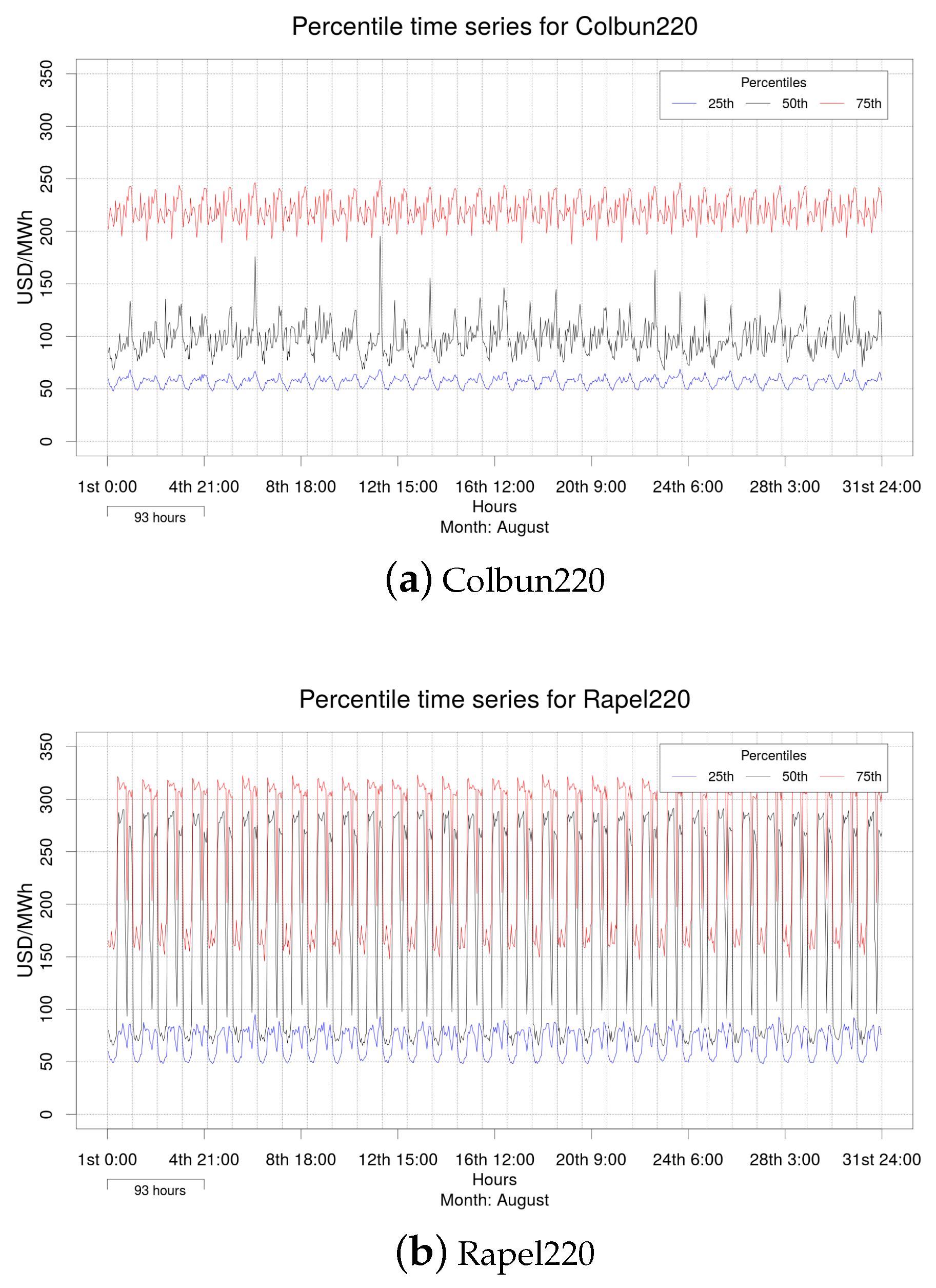
Once the spot price distributions were estimated, we followed the typical approach used for the economical-financial evaluation of projects and generated three scenarios: a pessimistic one (associated with the 25th percentile, P25, of the corresponding EDDP), a possible one (associated with the 50th percentile, P50, of the corresponding EDDP) and an optimistic one (associated with the 75th percentile, P75, of the corresponding EDDP). In Figure 8, we display the series associated with these three scenarios for two substations (Colbun220 and Rapel220) during the month of August. For Colbun220, there is a clear differentiation among the three scenarios, while for Rapel220, it holds that P50 and P75 tend to overlap.
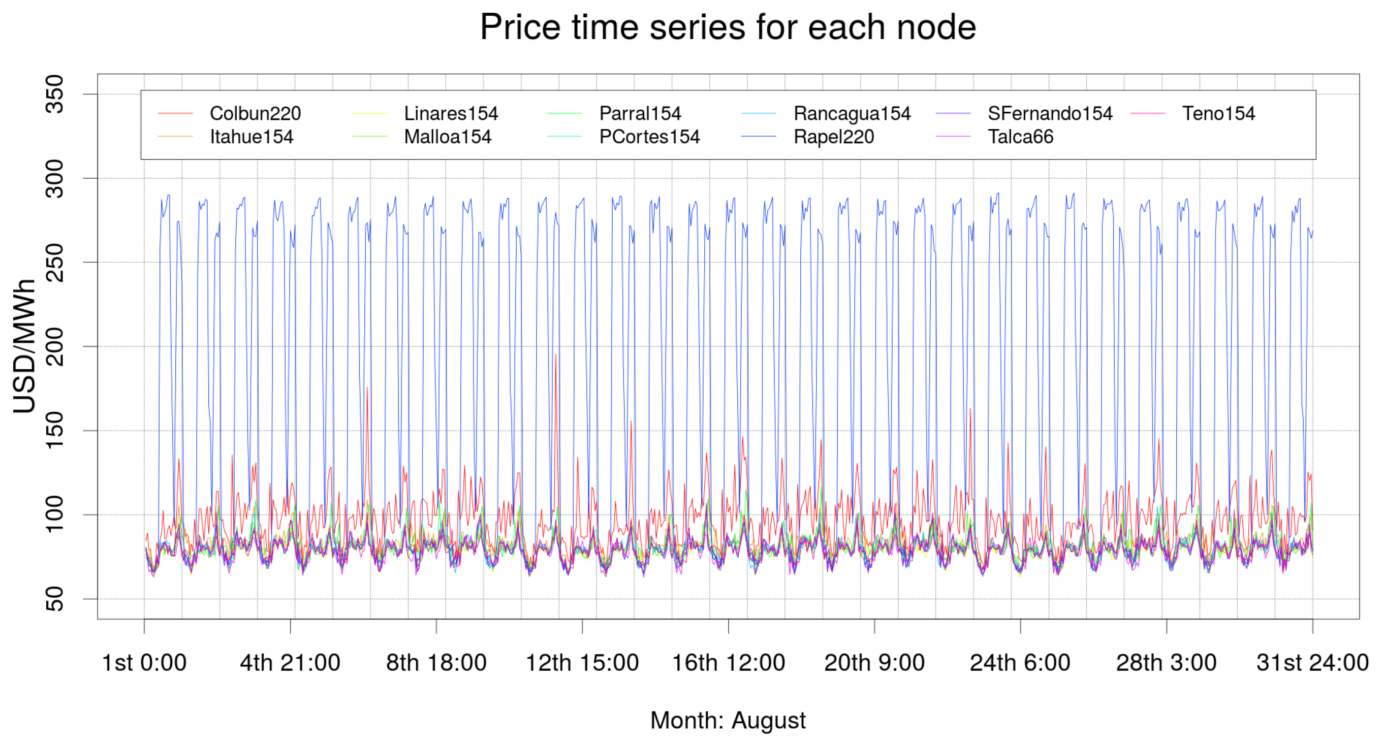
For complementing the results shown in Figure 8, we show in Figure 9 the time series associated with the 11 substations for P50 during the month of August. From this plot, it is clear that injecting energy in different substations leads to very different outcomes in terms of the collected revenue. While most of the prices fluctuate in the band 75–100 (USD/MWh), there are some cases (Rapel220 and Colbun220) where the price can be as high as 280 (USD/MWh).
The complex way that spot prices behave at different substations and at different times of the day reinforces the need for an accurate design tool that properly incorporates the nature of spot prices into an ad hoc mathematical optimization model.
4.3. Discussion and Results Analysis
In Section 4.2, we have described from where we have obtained or how we have estimated the parameters of the GTSELSP. In the remainder of this section, we present and discuss the results obtained when solving the GTSELSP and performing a sensitivity analysis.
Since the GTSELSP seeks for an optimal investment plan, in terms of the attained profit, the obtained solutions are not only measured by the underlying objective function value (annualized profit, measured by millions of USD per year), but also by its components (annualized investment costs and annualized incomes, measured by millions of USD per year) and by the corresponding internal rate of return (IRR, in percentage), which corresponds to the minimum discount rate that makes the project economically feasible (in this case, in a 30-year planning horizon).
4.3.1. Experimental Setting
We run our experiments on an Intel® CoreTM i7-4702MQ 2.20-GHz machine with 16 GB RAM and Ubuntu 16.04 LTS. The underlying GTSELSP instances were solved using ILOG® CPLEX® 12.6.3; we used default setting, except for the primal-dual gap, which was set to 0.2%.
4.3.2. Time Resolution
The first part of our computational analysis consists of determining which is the best time resolution for running the whole set of experiments. For such a purpose, we considered four time resolution structures:
- ‘12 × 1’: One year is characterized by 12 days, so that each day encodes one month. Since every day is comprised of 24 h, this setting yields .
- ‘4 × 7’: One year is characterized by four weeks, so that each week encodes three months. In this case, we have .
- ‘6 × 7’: One year is characterized by six weeks, so that each week encodes two months. In this case, we have .
- ‘12 × 7’: One year is characterized by 12 weeks, so that each week encodes one month. In this case, we have .
Since these four time resolution alternatives yield different sizes of set T, one would expect that the resulting MILP behaves numerically and computationally different.
In Figure 10a–c, we report the economical behavior (measured by the investment costs, incomes and IRR) of the solutions obtained when solving the GTSELSP for different scenarios of spot prices (i.e., P25, P50 and P75, respectively) and the different time resolutions. Surprisingly, we can see that regardless of the scenario, the solutions attained when using different time resolutions are quite similar in all economic dimensions (although, evidently, they differ when compared among scenarios).
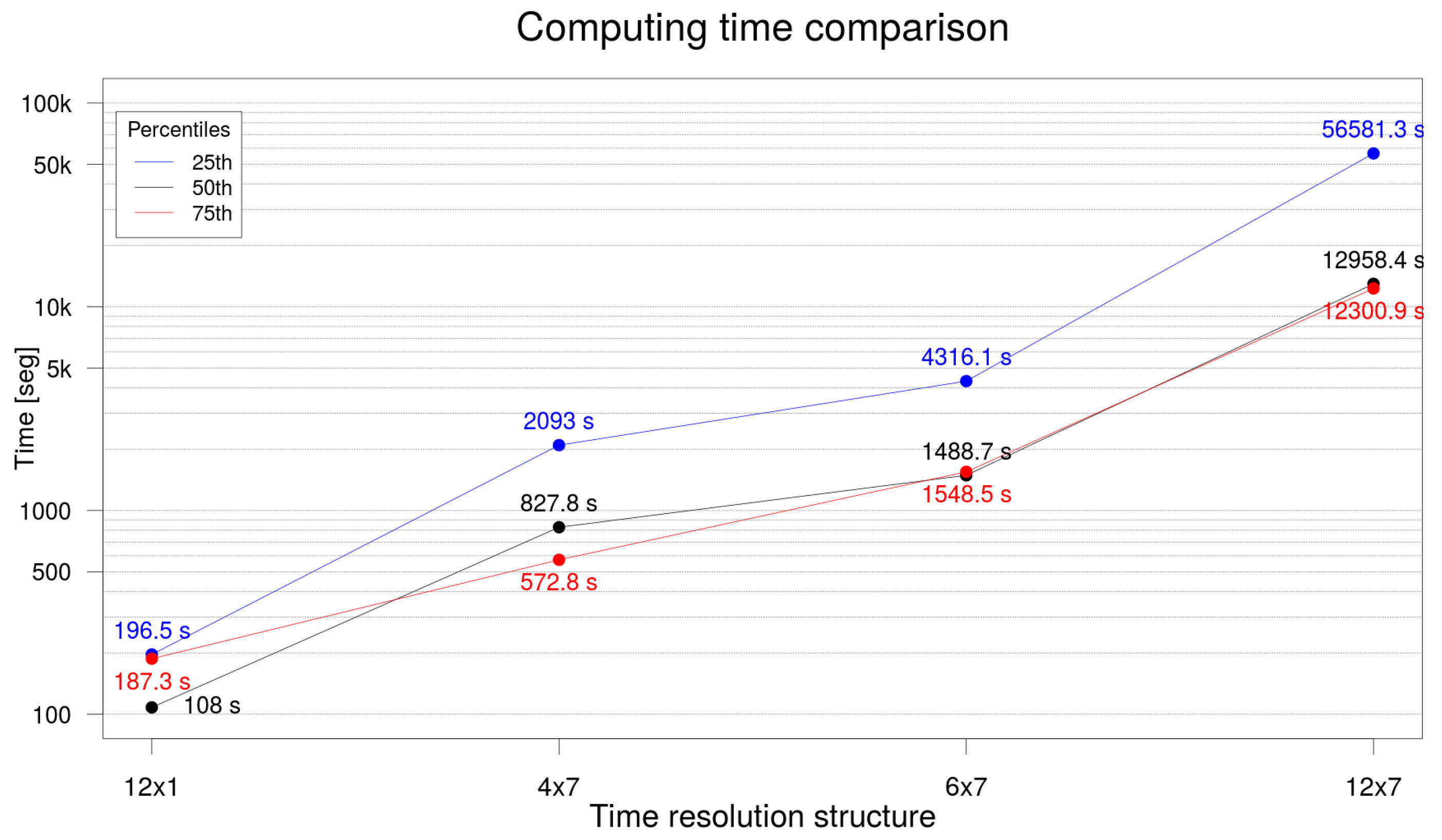
From the computational difficulty point of view, in Figure 11, we compare the computing time (vertical axis, in seconds) required for solving the MILP instances induced by the different time resolution structures (horizontal axis) and by the different price scenarios (colored lines). In this case, the impact of the different resolution alternatives is clear: the resolution ‘12 × 7’ induces resolutions times that are at least two orders of magnitude larger than those induced by ‘12 × 1’. Since the resolution times attained by ‘6 × 7’ are reasonable for the considered decision-making context, we use this time resolution as part of our default setting.
4.3.3. Spot Price Scenarios
As shown in Figure 10a–c, different price scenarios induce different economical performances. While the IRR attained when considering P25 (pessimistic scenario) is near 8.0%, the one attained for P50 (possible scenario) is almost 14.0%, and the one attained for P75 (optimistic scenario) can be above 28.0%. Interestingly, different scenarios of spot prices are not associated with noticeable differences in the investment cost (whose annualized value is shown by red lines), and the differences in the economical performance mainly depend on the different levels of collected revenues (blue lines).
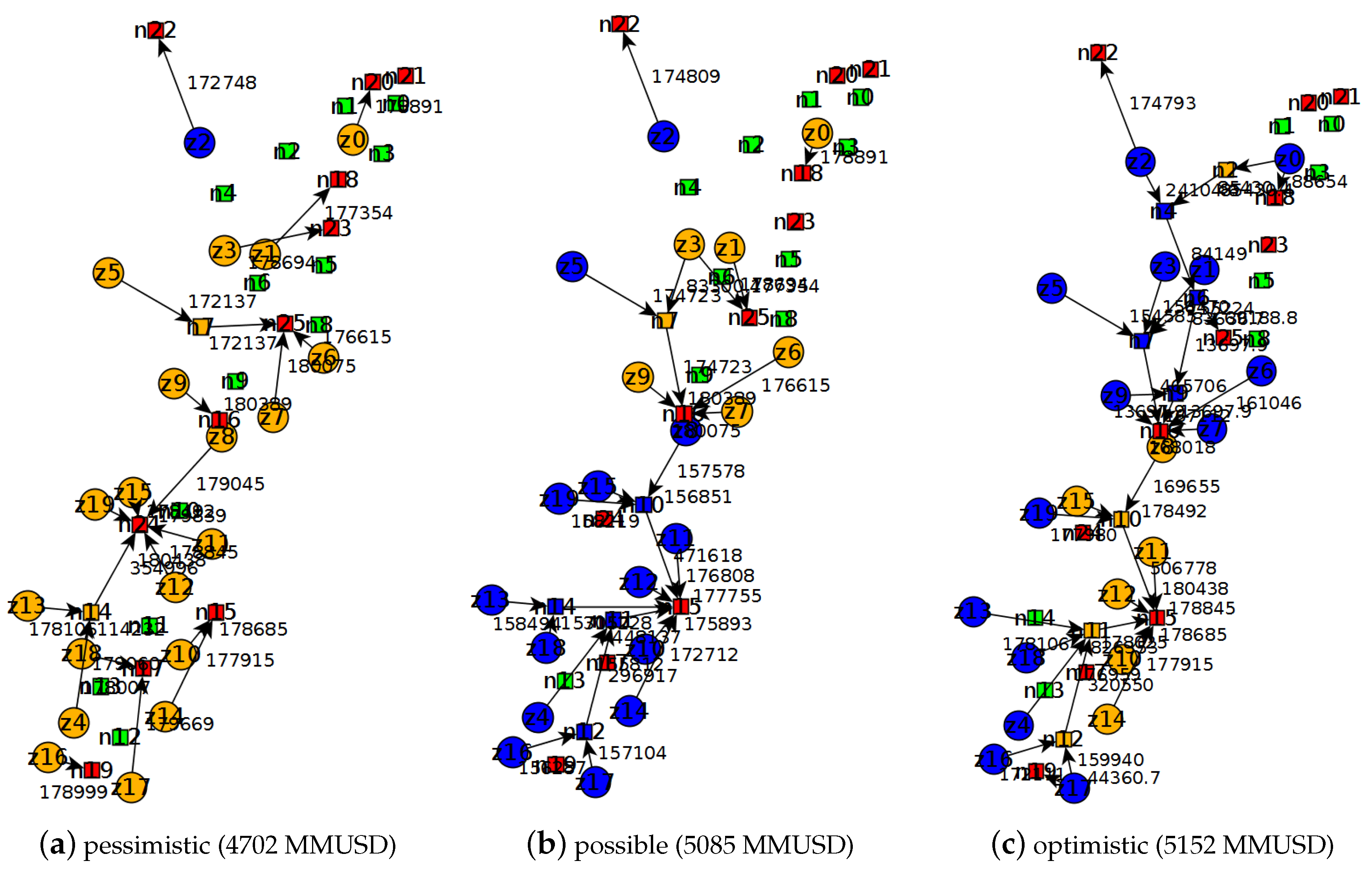
Although the investments do not fluctuate considerably according to the scenario, the infrastructure induced by these investments can be different, especially when comparing the one corresponding to P25 with respect to the one corresponding to P75 (i.e., the strategic design component of the GTSELSP solution differs when having different spot price realizations). In Figure 12, we report the solutions computed for these three scenarios (in the caption of each figure, we report total investment in MMUSD), the description of which is given as follows:
- The solution obtained for P25 (with a total investment of 4702 MMUSD) is comprised by 20 generation points (orange and blue circles), where an ESS facility is installed in only one of them (blue circle); these generation points inject the generated power through nine existing substations (red squares) and require one additional intermediate substation (orange square).
- The solution obtained for P50 (with a total investment of 5085 MMUSD) is comprised by 20 generation points, where ESS facilities are installed in 14 of them; these generation points inject the generated power through six existing substations and require five additional intermediate substations, and ESS facilities are installed in four of them (blue squares).
- The solution obtained for P75 (with a total investment of 5152 MMUSD) is comprised by 20 generation points, where ESS facilities are installed in 14 of them; these generation points inject the generated power through six existing substations and require eight additional intermediate substations, and ESS facilities are installed in four of them.
In light of the descriptions of the attained solutions and considering the values obtained for the IRR, the total incomes and the total investment costs, we consider that the scenario associated with P50 is a conservative way of capturing the spot price variability; hence, the possible scenario will be set as our default spot price realization.
Besides describing the effect of the spot price scenarios, one of the main outcomes of the analysis carried out is the important role that ESSs play within the designed solar power system. The solution shown in Figure 12b considers 1067 MWh of energy storage potential, while the generation potential is 4000 MWp. This solution shows that ESSs are an economically effective means of exploiting the generation from renewable sources, especially if they are incorporated within the system during its design stage.
4.3.4. Storage Technology
So far, we have considered that the ESS technology corresponds to PHS (which operates according to the parameters given in Table 2). However, decision-makers could be interested in knowing how the design and performance of the system changes when considering different storage technologies. For such a purpose, we solved the GTSELSP considering the four aforementioned storage systems; the produced solutions are shown in Figure 13. In the caption of each figure, we report in parenthesis the attained objective function value and the corresponding IRR. While the solutions obtained when considering ZEBRA and PBAC basically do not incorporate storage systems, the solutions associated with PHS and CAES incorporate ESS modules in many of the generation and intermediate points (totaling a storage capacity of 1067 and 733 MWh, respectively). Although from the objective function point of view, the PHS technology is associated with the best value (552 MMUSD), the results reported in Figure 13 make clear that recent technologies, such as ZEBRA, might boost the performance of power grids. The fact that no PBAC storage is installed should not be surprising, since this technology does not fit with the operational scheme of our design setting [34,35].
Additionally, the results reported in Figure 13, suggest that and are the most relevant parameters in the design strategy; both PHS and CAES allow larger charge and discharge flows (50 MW and 25 MW, respectively) than the ZEBRA and PBAC technologies (0.075 MW and 5 MW, respectively). This is explained by the fact that it is pointless to invest in a large capacity, i.e., a large value of , when it is impossible to charge or discharge such capacity. As a matter of fact, when looking at Figure 13c,d, we see many small CAES systems and fewer, but larger, PHS systems.
The considered technologies do not only differ in their operation, but also from the investment point of view (see Table 2). As can be seen from Figure 14 (ESS installation cost associated with the solutions reported in Figure 13), the investment in PHS is five-times higher than the one for CAES, and about 1000-times higher than the one for ZEBRA. This reveals that although PHS is an expensive technology, it pays back due to its efficiency in storing energy.
4.3.5. Sensitivity Analysis on Storage Parameters
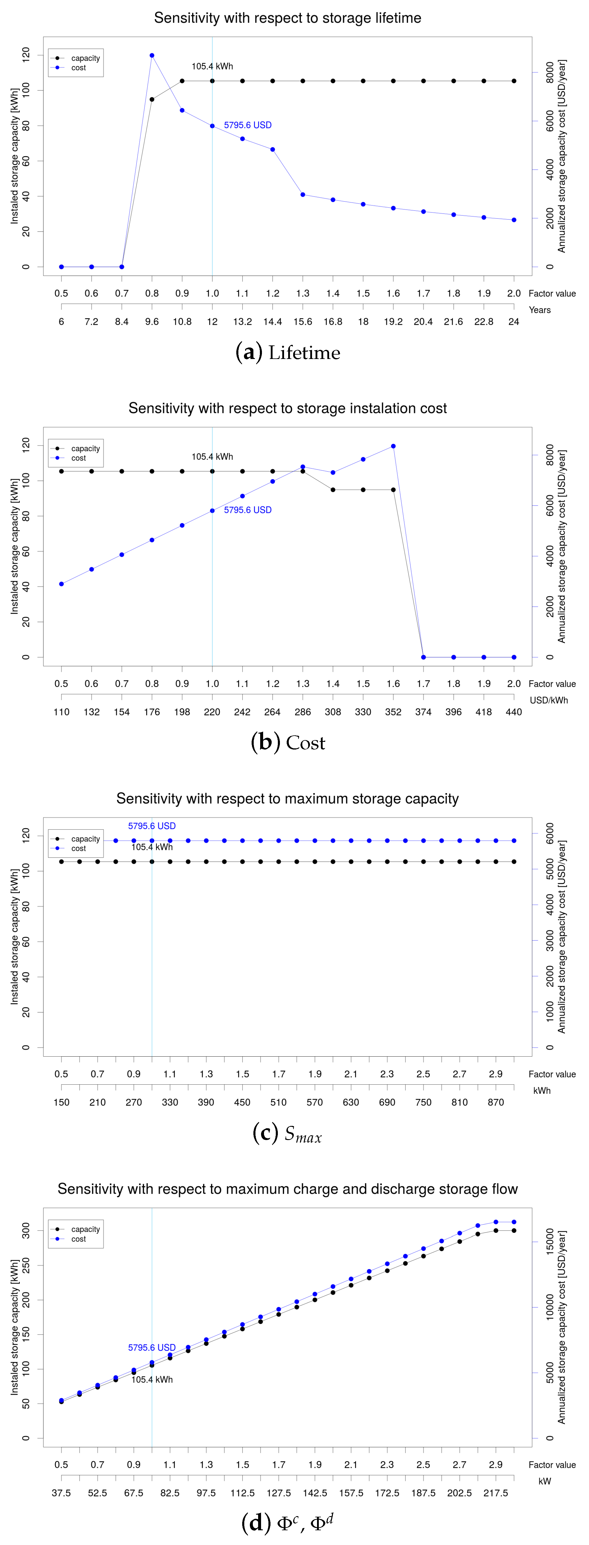
In light of the results presented above, we wanted to answer the following question: how sensitive are the ZEBRA storage installation decisions with respect to different values in the technology’s operative parameters?. By answering such a question, we would have an idea of how the ZEBRA technology should evolve in order to be economically feasible. Hence, we performed a sensitivity analysis on four parameters: the lifetime (years), the installation cost (USD/kWh), the maximum storage capacity (kWh) and the charge () and discharge rates () (kW). Using a ceteris paribus approach, we solved the GTSELSP for different values of the mentioned parameters and analyze how the installed storage (measured by capacity and total cost) changes as a consequence.
In Figure 15a, how the storage decisions would change if the ZEBRA lifetime goes from six (factor value = 0.5, i.e., half of the current lifetime of 12 years) to 24 years (factor value = 2, i.e., double the current lifetime of 12 years). Besides, the values associated with the current lifetime of 12 years are highlighted by a vertical line. From this plot, we can see that a lifetime of eight years makes the ZEBRA technology completely unpractical (installed capacity is 0 kWh). However, being able to extend the lifetime to double does not lead to any increase in the amount of installed capacity when compared to the original lifetime; only the present value of the total installation costs reduced significantly.
The sensitivity with respect to the installation cost is shown in Figure 15b, which is similar to Figure 15a. From this plot, we can see that an installation cost equal to or larger than 352 USD/KWh (1.6-times the original value of 220 USD/kWh) makes it economically impractical to use this technology. Nonetheless, even if the installation costs reduce to only half of the original value, i.e., falls to 110 USD/kWh, we would not install more capacity than that installed with the original value (highlighted by a vertical line).
The impact of modifying the maximum storage capacity can be analyzed from Figure 15d. In this case, it seems that the storage decisions are not sensitive to different values of ; even if it takes half or triple the original value, the storage capacity (and therefore, the cost) remains at 105.4 kWh. This result makes sense, since the original value of 0.3 MWh is already small.
Finally, we analyze how sensitive the storage decisions are with respect to the maximum charge and discharge flow. The plot shown in Figure 15d makes evident that these are the most influential parameters. There is a clear linear relation between the value of these parameters and the installed storage capacity. However, the increase in the installed capacity is bounded by kW, which coincides with the nominal maximum storage capacity kWh; therefore, having a larger charge and discharge flow capacity will not bring any change in the storage decision.
As a consequence of this sensitivity analysis, we can conclude that the key characteristics that comprise the viability of using ESSs within a large power system basically depend on allowing large amounts of stored energy () and the technological capacity of charging or discharging proportionally large amounts of energy ( and , respectively). According to this conclusion, we could affirm that the ZEBRA technology is unlikely to respond, at its current stage of development, to the needs of the power system as those considered within the scope of this paper.
5. Conclusions and Future Work
One of the most crucial challenges that society faces today corresponds to evolving our current power systems towards a scenario where renewable energies play a predominant role. This challenge brings several technological and strategic issues that have attracted the attention of researchers from different areas. In particular, several works have focused on the development of decision support tools for designing and sizing power systems based (completely or partially) on renewable sources. In this sense, the incorporation of energy storage systems as part of the decision-making scope is fundamental, and it leads to an additional level of modeling difficulty due to the complex interplay among the generation, transmission and storage decisions.
In this paper, we have presented a methodological framework for a strategic decision-making setting involving the design of a solar power system embedded within an existing large power grid. The developed tool relies on an optimization problem coined as the generation, transmission, storage energy location and sizing problem (GTSELSP), which allows on to compute economically-attractive investments given by the location and sizing of the generation and storage energy systems, along with the corresponding layout of transmission lines. By means of a real case study (located in the central region of Chile), characterized by carefully-curated data, we showed the potential of the developed tool for aiding long-term investment planning. The obtained solutions show that decision-makers could exploit ESSs if their location and sizing are defined, simultaneously, with the generation and transmission planning. Additionally, we showed how the proposed tool could be used to have an accurate measure of the impact of different ESS technologies. Furthermore, we also demonstrated the possible use of the developed tool for investigating how sensitive the storage decisions are with respect to the different operative parameters of a given technology; this latter characteristic is particularly important for those researchers working on improving existing storage technologies.
An interesting path for future work would be to devise a more complex setting in which the design power system is evaluated by a proxy of its actual functioning regime; for instance, by solving a unit commitment problem that incorporates the designed power system. Such an approach is likely to lead to an iterative scheme that shall provide a much more accurate evaluation of the designed power system.
Acknowledgments
David Olave-Rojas and Eduardo Álvarez-Miranda acknowledge the support of the Chilean Council of Scientific and Technological Research (FONDECYT Grant No. 11140060 and Complex Engineering Systems Institute ICM:P-05-004-F/CONICYT:FB0816). The authors would like to thank the support of C. Wander and R. Fuentes-Ryks from Vivest Energías Renovables S.A.
Author Contributions
David Olave-Rojas contributed with the problem definition and formulation, performed most of data processing, computational implementation, experimental design, results analysis, and wrote most of the paper. Eduardo Álvarez-Miranda contributed with the problem definition and formulation, and partially contributed with the computational implementation, experimental design and results analysis. Alejandro Rodríguez performed the bootstrapping analysis of spot prices, and partially contributed with results analysis. Claudio Tenreiro partially contributed with the problem definition, the experimental design and results analysis.
Conflicts of Interest
The authors declare no conflict of interest.
References
- International Energy Agency (IEA). Key World Energy Statistics 2015; Technical Report; International Energy Agency: Vienna, Austria, 2015. [Google Scholar]
- Carlyle, R. How big are the currently known oil reserves and what are the chances of finding new ones?—Forbes. Available online: http://www.forbes.com/sites/quora/2013/03/27/how-big-are-the-currently-known-oil-reserves-and-what-are-the-chances-of-finding-new-ones/ (accessed on 21 July 2016).
- Tully, A. How long will world’s oil reserves last? 53 Years, Says BP. Available online: http://www.csmonitor.com/Environment/Energy-Voices/2014/0714/How-long-will-world-s-oil-reserves-last-53-years-says-BP (accessed on 21 July 2016).
- Petroleum, B.B. Oil Reserves | About BP | BP Global. Available online: http://www.bp.com/en/global/corporate/energy-economics/statistical-review-of-world-energy/oil/oil-reserves.html (accessed on 21 July 2016).
- Roboam, X. (Ed.) Integrated Design by Optimization of Electrical Energy Systems; Wiley-ISTE: Hoboken, NJ, USA, 2012. [Google Scholar]
- Suazo-Martínez, C.; Pereira-Bonvallet, E.; Palma-Behnke, R. A simulation framework for optimal energy storage sizing. Energies 2014, 7, 3033–3055. [Google Scholar] [CrossRef]
- Kim, J.; Powell, W. Optimal energy commitments with storage and intermittent supply. Oper. Res. 2011, 59, 1347–1360. [Google Scholar] [CrossRef]
- Koltsaklis, N.; Georgiadis, M. A multi-period, multi-regional generation expansion planning model incorporating unit commitment constraints. Appl. Energy 2015, 158, 310–331. [Google Scholar] [CrossRef]
- Jiang, R.; Wang, J.; Guan, Y. Robust unit commitment with wind power and pumped storage hydro. IEEE Trans. Power Syst. 2012, 27, 800–810. [Google Scholar] [CrossRef]
- Dehghan, S.; Amjady, N. Robust transmission and energy storage expansion planning in wind farm-integrated power systems considering transmission switching. IEEE Trans. Sustain. Energy 2016, 7, 765–774. [Google Scholar] [CrossRef]
- MacRae, C.; Ozlen, M.; Ernst, A.; Behrens, S. Locating and sizing energy storage systems for distribution feeder expansion planning. In Proceedings of the TENCON 2015—2015 IEEE Region 10 Conference, Macao, China, 1–4 November 2015; pp. 1–6. [Google Scholar]
- Bradbury, K.; Pratson, L.; Patiño-Echeverri, D. Economic viability of energy storage systems based on price arbitrage potential in real-time US electricity markets. Appl. Energy 2014, 114, 512–519. [Google Scholar] [CrossRef]
- Berrada, A.; Loudiyi, K. Operation, sizing, and economic evaluation of storage for solar and wind power plants. Renew. Sustain. Energy Rev. 2016, 59, 1117–1129. [Google Scholar] [CrossRef]
- Xiong, P.; Singh, C. Optimal planning of storage in power systems integrated with wind power generation. IEEE Trans. Sustain. Energy 2016, 7, 232–240. [Google Scholar] [CrossRef]
- Rahmann, C.; Palma-Behnke, R. Optimal allocation of wind turbines by considering transmission security constraints and power system stability. Energies 2013, 6, 294–311. [Google Scholar] [CrossRef]
- Jakus, D.; Krstulovic, J.; Vasilj, J. Algorithm for optimal wind power plant capacity allocation in areas with limited transmission capacity. Int. Trans. Electr. Energy Syst. 2014, 24, 1505–1520. [Google Scholar] [CrossRef]
- Qi, W.; Liang, Y.; Shen, Z. Joint planning of energy storage and transmission for wind energy generation. Oper. Res. 2015, 63, 1280–1293. [Google Scholar] [CrossRef]
- Ghofrani, M.; Arabali, A.; Etezadi-Amoli, M.; Fadali, M. A framework for optimal placement of energy storage units within a power system with high wind penetration. IEEE Trans. Sustain. Energy 2013, 4, 434–442. [Google Scholar] [CrossRef]
- Oh, H. Optimal planning to include storage devices in power systems. IEEE Trans. Power Syst. 2011, 26, 1118–1128. [Google Scholar] [CrossRef]
- Jabr, R.; Džafić, I.; Pal, B. Robust optimization of storage investment on transmission networks. IEEE Trans. Power Syst. 2015, 30, 531–539. [Google Scholar] [CrossRef]
- Wang, H.; Huang, J. Hybrid renewable energy investment in microgrid. In Proceedings of the 2014 IEEE International Conference on Smart Grid Communications, Venice, Italy, 3–6 November 2014; pp. 602–607. [Google Scholar]
- Wang, H.; Huang, J. Joint investment and operation of microgrid. IEEE Trans. Smart Grid 2017, 8, 833–845. [Google Scholar] [CrossRef]
- Wang, H.; Huang, J. Cooperative planning of renewable generations for interconnected microgrids. IEEE Trans. Smart Grid 2016, 7, 2486–2496. [Google Scholar] [CrossRef]
- Ciabattoni, L.; Ferracuti, F.; Grisostomi, M.; Ippoliti, G.; Longhi, S. Fuzzy logic based economical analysis of photovoltaic energy management. Neurocomputing 2015, 170, 296–305. [Google Scholar] [CrossRef]
- Ministerio de Energía de Chile. Explorador de Energía Solar. 2011. Available online: http://walker.dgf.uchile.cl/Explorador/Solar3/ (accessed on 03 May 2016). (In Spanish).
- Fuentes-Ryks, R.; Wander, C. Technical Information. Personal communication, Vivest Energías Renovables S.A.. 2016. [Google Scholar]
- Coordinador Eléctrico Nacional. Información Técnica Centrales SING. 2016. Available online: http://cdec2.cdec-sing.cl/pls/portal/cdec.pck_web_coord_elec.sp_pagina?p_id=5187 (accessed on 20 May 2016). (In Spanish).
- Dirección de Planificación y Desarrollo CDEC-SIC. Determinación de Puntos de Conexión STT. Technical Report. Coordinador Eléctrico Nacional: Santiago, Chile, 2015. Available online: https://sic.coordinadorelectrico.cl/wp-content/uploads/2015/07/Determinación-de-puntos-de-conexión-STT.pdf(accessed on 4 May 2016). (In Spanish)
- ABB AB. It’s Time to Connect-HVDC Light©, 7th ed.; Grid Systems-NVDC: Ludvika, Sweden, 2013. [Google Scholar]
- European Network of Transmission System Operators for Electricity. Offshore Transmission Technology; Technical Report Prepared by the Regional Group North Sea for the NSCOGI; ENTSOE: Brussels, Belgium, 2011. [Google Scholar]
- Lancheros, C. Transmission Systems for Offshore Wind Farms: A Technical, Enviromental and Economic Assessment. Master’s Thesis, Hamburg University of Technology, Hamburg, Germany, 2013. [Google Scholar]
- Fischetti, M.; Leth, J.; Borchersen, A. A Mixed-Integer Linear Programming approach to wind farm layout and inter-array cable routing. In Proceedings of the 2015 American Control Conference (ACC), Chicago, IL, USA, 1–3 July 2015; pp. 5907–5912. [Google Scholar]
- Van Eeckhout, B.; Van Hertem, D.; Reza, M.; Srivastava, K.; Belmans, R. Economic comparison of VSC, HVDC and HVAC as transmission system for a 300 MW offshore wind farm. Eur. Trans. Electr. Power 2010, 20, 661–671. [Google Scholar] [CrossRef]
- Chen, H.; Cong, T.; Yang, W.; Tan, C.; Li, Y.; Ding, Y. Progress in electrical energy storage system: A critical review. Prog. Nat. Sci. 2009, 19, 291–312. [Google Scholar] [CrossRef]
- Cho, J.; Jeong, S.; Kim, Y. Commercial and research battery technologies for electrical energy storage applications. Prog. Energy Combust. Sci. 2015, 48, 84–101. [Google Scholar] [CrossRef]
- Coordinador Eléctrico Nacional. Programación Semanal CDEC SIC. 2016. Available online: https://sic.coordinadorelectrico.cl/informes-y-documentos/fichas/operacion-programada-2/ (accessed on 3 May 2016).
- Pascual, L.; Romo, J.; Ruiz, E. Bootstrap predictive inference for ARIMA processes. J. Time Ser. Anal. 2004, 25, 449–465. [Google Scholar] [CrossRef] [Green Version]
- Pascual, L.; Romo, J.; Ruiz, E. Bootstrap prediction intervals for power-transformed time series. Int. J. Forecast. 2005, 21, 219–235. [Google Scholar] [CrossRef] [Green Version]
Figure 1.
Graphical representation of the studied instance. We use squares to represent to substations; circles to represent generation zones (V1); green color indicates possible substations (V2); and red color for existing substations (O).
Figure 1.
Graphical representation of the studied instance. We use squares to represent to substations; circles to represent generation zones (V1); green color indicates possible substations (V2); and red color for existing substations (O).
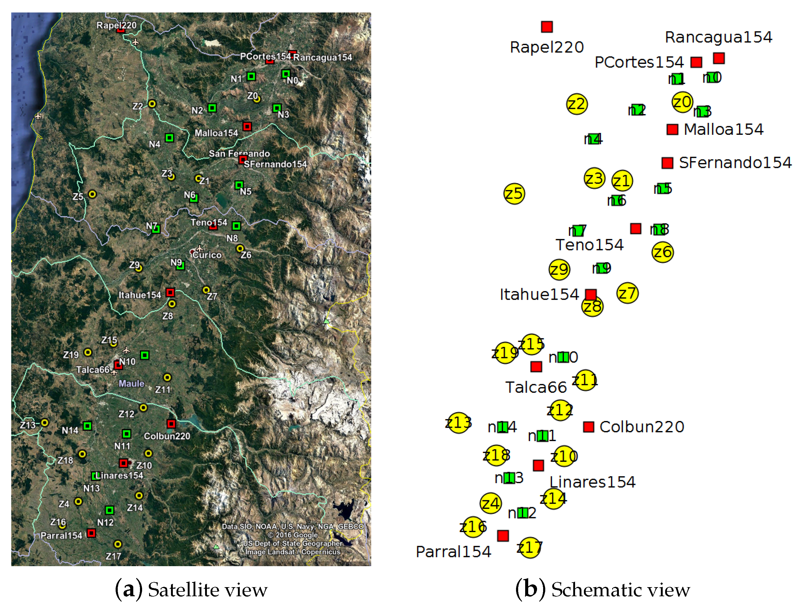
Figure 2.
Representation of available average radiation for each studied zone.

Figure 3.
Relationship between power and construction cost for PV power plants.
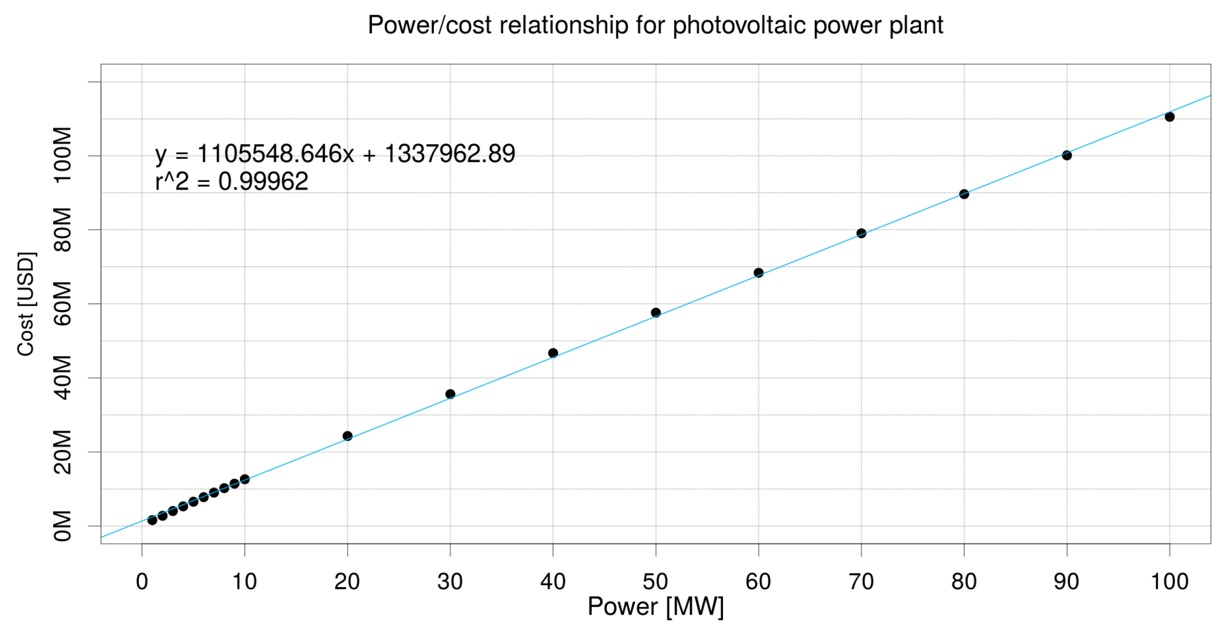
Figure 4.
Relationship between power and construction cost for a 1 (km) transmission line.

Figure 5.
Relationship between power and construction cost for substations.

Figure 6.
Empirical density distribution spot prices for Itahue154 in four representative days of the year.
Figure 6.
Empirical density distribution spot prices for Itahue154 in four representative days of the year.
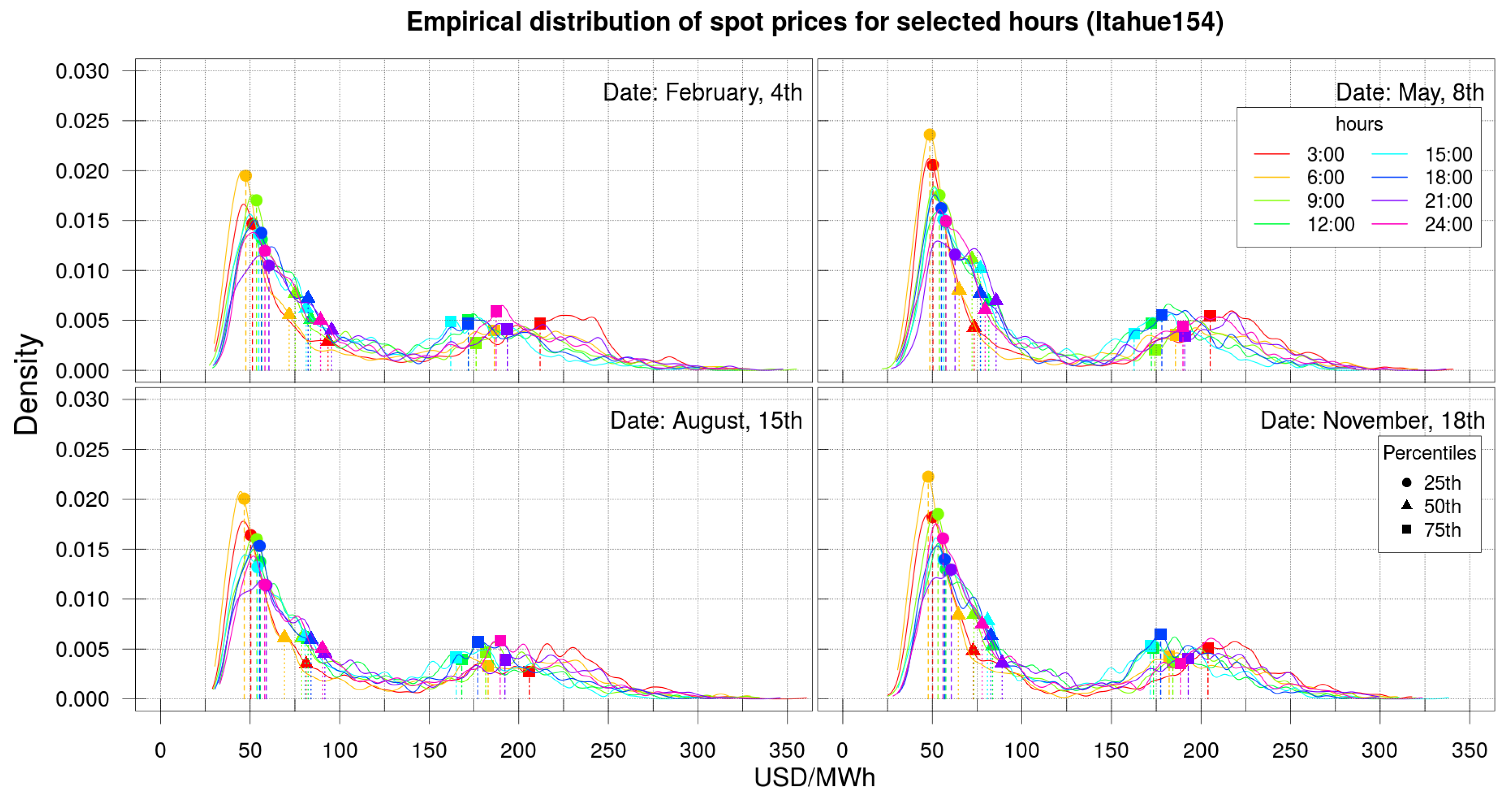
Figure 7.
Empirical density distribution spot prices for Rapel220 in four representative days of the year.
Figure 7.
Empirical density distribution spot prices for Rapel220 in four representative days of the year.
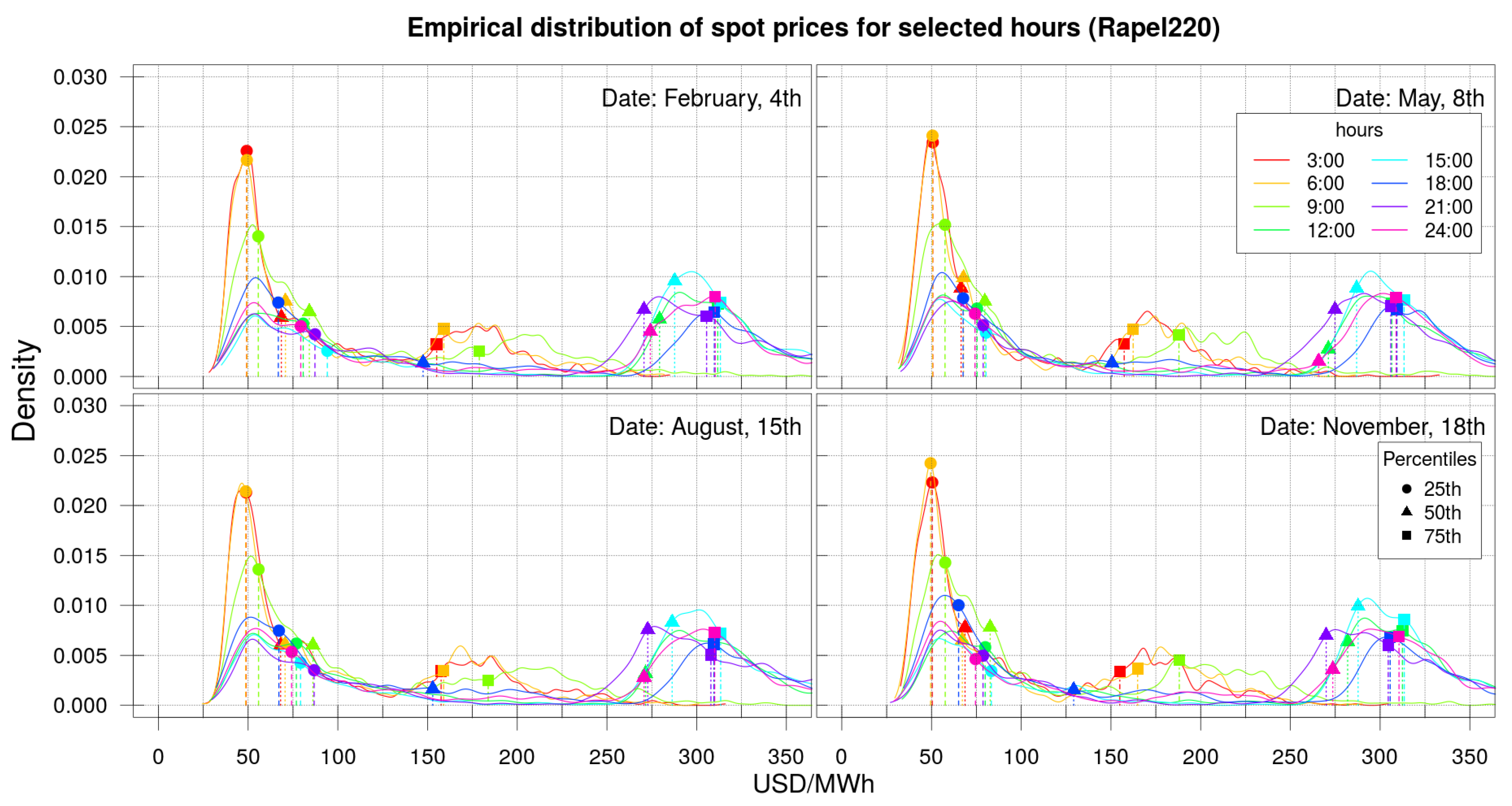
Figure 8.
Percentile time series for (a) Colbun220 and (b) Rapel220 for the month of August.

Figure 9.
Spot price time series for each existing substation on the studied region for P50 and for the whole month of August.
Figure 9.
Spot price time series for each existing substation on the studied region for P50 and for the whole month of August.

Figure 10.
Comparison between economical indicators attained for different time resolution structures and scenarios. (a) Percentile 25; (b) Percentile 50; (c) Percentile 75.
Figure 10.
Comparison between economical indicators attained for different time resolution structures and scenarios. (a) Percentile 25; (b) Percentile 50; (c) Percentile 75.
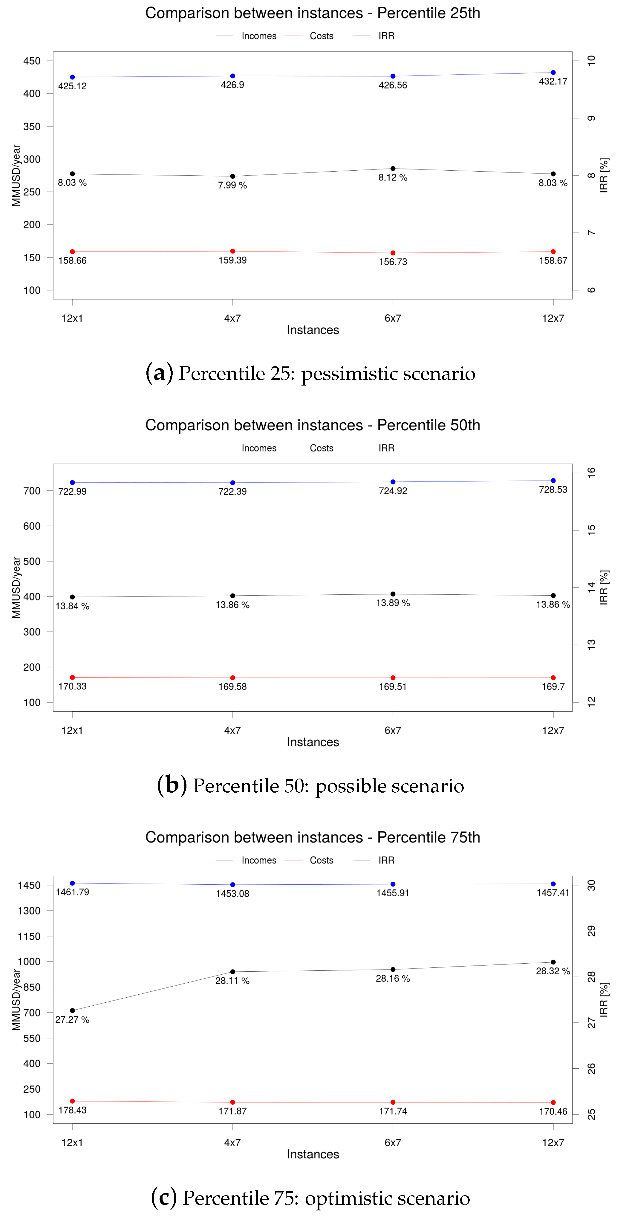
Figure 11.
Computing time comparison for different time resolution structures.

Figure 12.
Generation, Transmission, Storage Energy Location and Sizing Problem (GTSELSP) solutions when using PHS technology and considering three spot price scenarios (squares = substations (V2 ∪ O); circles = generation zones (V1); green = unselected; orange = selected; red = sales node (O); blue = storage system). (a) pessimistic (4702 MMUSD; (b) possible (5085 MMUSD); (c) optimistic (5152 MMUSD).

Figure 13.
Results for technological ESS comparison in P50 (squares = substations (V2 ∪ O); circles = generation zones (V1); green = unselected; orange = selected; red = sales node (O); blue = storage system).
Figure 13.
Results for technological ESS comparison in P50 (squares = substations (V2 ∪ O); circles = generation zones (V1); green = unselected; orange = selected; red = sales node (O); blue = storage system).
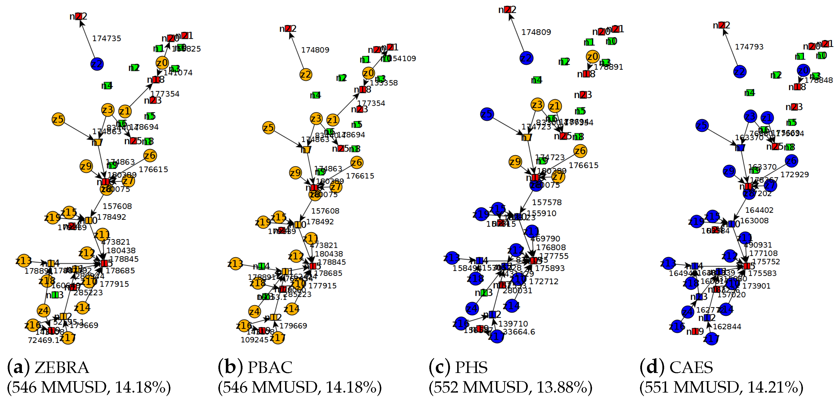
Figure 14.
Investment results for the studied ESS technologies in P50.
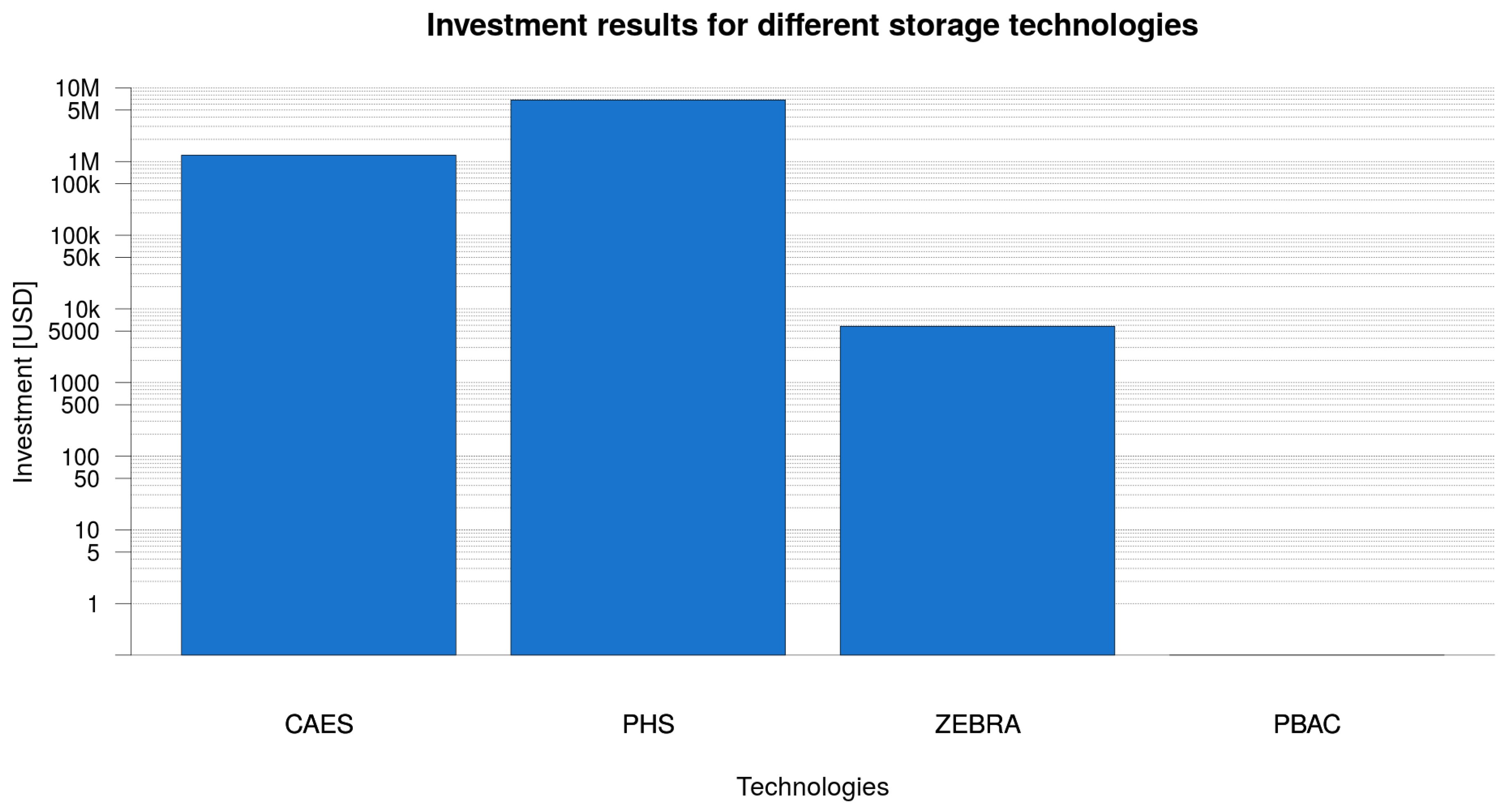
Figure 15.
Sensitivity analysis results for four ESS parameters: (a) lifetime, (b) cost, (c) max. storage capacity and (d) charge/discharge storage flows. Lines represent the aggregated installed ESS cost and capacity for ZEBRA technology.
Figure 15.
Sensitivity analysis results for four ESS parameters: (a) lifetime, (b) cost, (c) max. storage capacity and (d) charge/discharge storage flows. Lines represent the aggregated installed ESS cost and capacity for ZEBRA technology.

Table 1.
Summary of the literature related to energy systems’ planning incorporating renewable and conventional generation, transmission and storage sizing and design. Op., operational profiles; Tech., technological assessment.
Table 1.
Summary of the literature related to energy systems’ planning incorporating renewable and conventional generation, transmission and storage sizing and design. Op., operational profiles; Tech., technological assessment.
| Reference | Storage | Generation | Transmission | ||||||
|---|---|---|---|---|---|---|---|---|---|
| Capacity | Location | Others | Capacity | Location | Others | Layout | Capacity | Flow | |
| [6] | ✓ | ||||||||
| [7] | Op. | Op. | |||||||
| [8] | Op. | ||||||||
| [9] | Op. | ||||||||
| [10] | ✓ | ✓ | Op. | ✓ | |||||
| [11] | ✓ | ✓ | Op. | ✓ | |||||
| [12] | ✓ | Tech. | |||||||
| [13] | ✓ | Op. and Tech. | |||||||
| [14] | ✓ | ✓ | Op. | ||||||
| [15] | ✓ | Tech. | |||||||
| [16] | ✓ | ✓ | ✓ | ✓ | |||||
| [17] | ✓ | ✓ | ✓ | ✓ | |||||
| [18] | ✓ | ✓ | |||||||
| [19] | ✓ | Op. | ✓ | ||||||
| [20] | ✓ | ✓ | ✓ | ||||||
| [21] | ✓ | Op. and Tech. | |||||||
| [22] | ✓ | Op. | ✓ | Op. and Tech. | |||||
| [23] | Op. | ✓ | ✓ | Op. and Tech. | |||||
| our work | ✓ | ✓ | Op. and Tech. | ✓ | ✓ | Connect. | ✓ | ✓ | ✓ |
Table 2.
Different technologies for ESS that we consider in this work. ZEBRA, Zeolite Battery Research Africa battery of sodium-nickel chloride cell; PBAC, Pb-acid batteries; PHS, pumped hydroelectric storage; CAES, compressed air energy storage.
Table 2.
Different technologies for ESS that we consider in this work. ZEBRA, Zeolite Battery Research Africa battery of sodium-nickel chloride cell; PBAC, Pb-acid batteries; PHS, pumped hydroelectric storage; CAES, compressed air energy storage.
| (MWh) | , (%) | , (MW) | (%) | Cost (USD/MWh) | Lifetime (Years) | Reference | |
|---|---|---|---|---|---|---|---|
| ZEBRA | 0.3 | 94.9 | 0.075 | 25 | 220,000 | 12 | [34] |
| PBAC | 20 | 86.6 | 5 | 40 | 450,000 | 10 | [26,34,35] |
| PHS | 200 | 92.0 | 50 | 10 | 200,000 | 30 | [34] |
| CAES | 200 | 89.0 | 25 | 10 | 50,000 | 30 | [34] |
© 2017 by the authors. Licensee MDPI, Basel, Switzerland. This article is an open access article distributed under the terms and conditions of the Creative Commons Attribution (CC BY) license (http://creativecommons.org/licenses/by/4.0/).
Share and Cite
MDPI and ACS Style
Olave-Rojas, D.; Álvarez-Miranda, E.; Rodríguez, A.; Tenreiro, C. An Optimization Framework for Investment Evaluation of Complex Renewable Energy Systems. Energies 2017, 10, 1062. https://doi.org/10.3390/en10071062
AMA Style
Olave-Rojas D, Álvarez-Miranda E, Rodríguez A, Tenreiro C. An Optimization Framework for Investment Evaluation of Complex Renewable Energy Systems. Energies. 2017; 10(7):1062. https://doi.org/10.3390/en10071062
Chicago/Turabian StyleOlave-Rojas, David, Eduardo Álvarez-Miranda, Alejandro Rodríguez, and Claudio Tenreiro. 2017. "An Optimization Framework for Investment Evaluation of Complex Renewable Energy Systems" Energies 10, no. 7: 1062. https://doi.org/10.3390/en10071062
Note that from the first issue of 2016, this journal uses article numbers instead of page numbers. See further details here.