A Novel Workflow for Geothermal Prospectively Mapping Weights-of-Evidence in Liaoning Province, Northeast China

1
College of Earth Science, Jilin University, Changchun 130061, China
2
Xinjiang Uyghur Autonomous Region Academy of Surveying and Mapping, No. 231 Sandaowan East Road, Urumchi 830002, China
3
College of Information Sciences and Technology, Chengdu University of Technology, Chengdu 610059, China
*
Author to whom correspondence should be addressed.
Energies 2017, 10(7), 1069; https://doi.org/10.3390/en10071069
Submission received: 3 July 2017
/
Revised: 18 July 2017
/
Accepted: 19 July 2017
/
Published: 22 July 2017
(This article belongs to the Section L: Energy Sources)
Abstract
:Geological faults are highly developed in the eastern Liaoning Province in China, where Mesozoic granitic intrusions and Archean and Paleoproterozoic metamorphic rocks are widely distributed. Although the heat flow value in eastern Liaoning Province is generally low, the hot springs are very developed. It is obvious that the faults have significant control over the distribution of hot springs, and traditional methods of spatial data analysis such as WofE (weight of evidence) usually do not take into account the direction of the distribution of geothermal resources in the geothermal forecast process, which seriously affects the accuracy of the prediction results. To overcome the deficiency of the traditional evidence weight method, wherein it does not take the direction of evidence factor into account, this study put forward a combination of the Fry and WofE methods, Fry-WofE, based on geological observation, gravity, remote sensing, and DEM (digital elevation model) multivariate data. This study takes eastern Liaoning Province in China as an example, and the geothermal prospect was predicted respectively by the Fry-WofE and WofE methods from the statistical data on the spatial distribution of the exposed space of geothermal anomalies the surface. The result shows that the Fry-WofE method can achieve better prediction results when comparing the accuracy of these two methods. Based on the results of Fry-WofE prediction and water system extraction, 13 favorable geothermal prospect areas are delineated in eastern Liaoning Province. The Fry-WofE method is effective in study areas where the geothermal distribution area is obviously controlled by the fault. We provide not only a new method for solving the similar issue of geothermal exploration, but also a new insight into the distribution of geothermal resources in Liaoning Province.
1. Introduction
Geothermal resources, as a clean energy source, have received significant attention around the world, and the assessment of regional geothermal resources is the basis for the effective development and utilization of geothermal resources [1]. The prospect evaluation of geothermal resources can be estimated by a spatial information analysis method, which is effective, requires relatively less investment, and is based on integrating the multidisciplinary data of remote sensing, geology, geophysics, and geography. Scientists from all over the world have done a lot of research in this field. Noorollahi et al. [2] used the geological and geomorphological data of northwest Sabalan, drawing a rose diagram of the fault strikes. The multiple-criteria decision-making method is used to calculate favorable positions for geothermal resources exploitation and drilling. Moghaddam et al. [3] analyzed the geothermal resources in the Akita and Iwate Provinces with the WofE method, discussing its spatial distribution characteristics and correlated factors based on a Fry rose diagram. A Boolean logic model and a fuzzy system model were used to generate the map of the geothermal distribution in his study area. Wibowo et al. [4] also utilized the Fry method to explore the spatial distribution of geothermal resources in West Java and did evaluation with the WOFE method.
The WofE method has been widely used in the geological industry [5,6,7,8,9,10,11]. In addition, many scholars put forward the Fuzzy WofE model [12,13,14,15,16,17,18], Boost WofE model [19], and SVM-WofE (support vector machine-weight of evidence) model [20,21] for the shortcomings of the accuracy loss with the weighting of evidence. However, no one has proposed an algorithm for the quantitative weighting of linear features by direction. The geothermal field in Liaoning province is mainly controlled by geological faults [22,23]. Many scholars used the traditional geological method [24,25,26] and the borehole temperature measurement method [27] to analyze the influence of the regional tectonic system on the geothermal resources in the east of Liaoning Province. There is much less research on the distribution of a wide range of regularities in the hot springs in Liaoning province, but the traditional multivariate information statistical method does not take into account the direction of the evidence weighing factors. The WofE method is an example. In the absence of processing of the fault direction, the prediction error increases significantly. The prediction response level of the fault in the high potential direction will be lowered by the fault in the low potential direction, which can reduce the overall prediction accuracy [28]. This issue appears not only in the WofE method, but also in many multivariate analysis algorithms. To improve the utilization of data, the preprocessing of the data itself is bound to be one of the main development directions of the algorithm analysis in the future [29].
The faults are very developed in the eastern part of Liaoning Province in China, where Mesozoic intrusions and Archean metamorphic rocks are widely distributed. Although the geothermal characteristics indicate generally low terrestrial heat flow values in Liaoning province, the hot springs, for example, China’s famous East-soup hot spring, are utterly developed in the study area [22,30,31]. By integrating multivariate data, including geophysical, geological, and remote sensing data, we propose a new method and workflow for evaluating geothermal resources based on combining the Fry and WofE methods. The application of geothermal prospect assessment in the eastern part of Liaoning province shows that this method can effectively determine the favorable area for geothermal development. This paper mainly discusses the algorithm optimization of the geothermal anomaly and its distribution, and shows the improvement of the new method compared with traditional WofE method by demonstrating the computational process, the implementation procedure, and the predictive accuracy.
Research shows that the appropriate data processing method, which considers the spatial distribution characteristics of objects separately as an influence factor, will play a significantly positive role for the results of the WofE model in the course of dealing with the spatial distribution of geothermal anomalies. In the experiment, a satisfactory result shows that the prediction accuracy of the fault data processed by the Fry method is 12.1% higher than the accuracy obtained by directly using WofE method. At the same time, we use this more accurate prediction method to replan the geothermal prospective area in the eastern part of Liaoning Province. 13 prospective areas are divided, five of which are new prediction areas.
2. Geological Background of the Study Area
The eastern part of Liaoning Province is located in the northeast of China. The study area belongs to the northeast section of the eastern landmass of North China Craton (NCC), with an area of 24,262.9 km2. The geothermal heat flow in the study area is generally low, but there are many hot springs. Most of the hot springs in the study area are distributed along faults, which indicates that the distribution of geothermal fields is obviously controlled by faults [32,33]. Intrusive masses, metamorphic rocks, and faults are widely distributed in the study area, with NE-trending faults being well developed, among which the main fault distribution is visible in Figure 1. The major NE-trending faults there include ZH (Zhuanghe-Huanren), SF (Sipingjie-Fengcheng), EC (Erpengdianzi-Changdian), YL (Yalu River), and LQ (Liujiahe-Qingduizi). The NE (Northeast)-trending faults that are the main controlling structures in eastern Liaoning province divide the tectonic regions into long strip faulted blocks and control the formation and development of modern landforms. The later formed NE-trending faults cut through the original structure. From the formation stage, the EW (Eastwest)-trending faults formed earliest [34]; they are mainly due to activity in the early Proterozoic [35]; Most of the NE-trending faults were formed during Indosinian movements at the end of the middle of the Triassic period [36]. The crustal activity reached its peak in the early Cretaceous period. Eastern China, including the study area, was affected by east-west compressional movement, which is caused by north-south force-coupling [37]. Thus, NE strike slip faults and NW-NNW (Northwest-North Northeast) trending tensional faults occur [38].
3. Geothermal Resources Prospective Prediction with Fry-WofE Methods and Processes
3.1. Processes
The Fry-WofE method is used to predict the geothermal potential on the basis of multidisciplinary data after processing the hot spring through Fry analysis. The result shows a higher prediction accuracy after processing the fracture layer data by using this method.
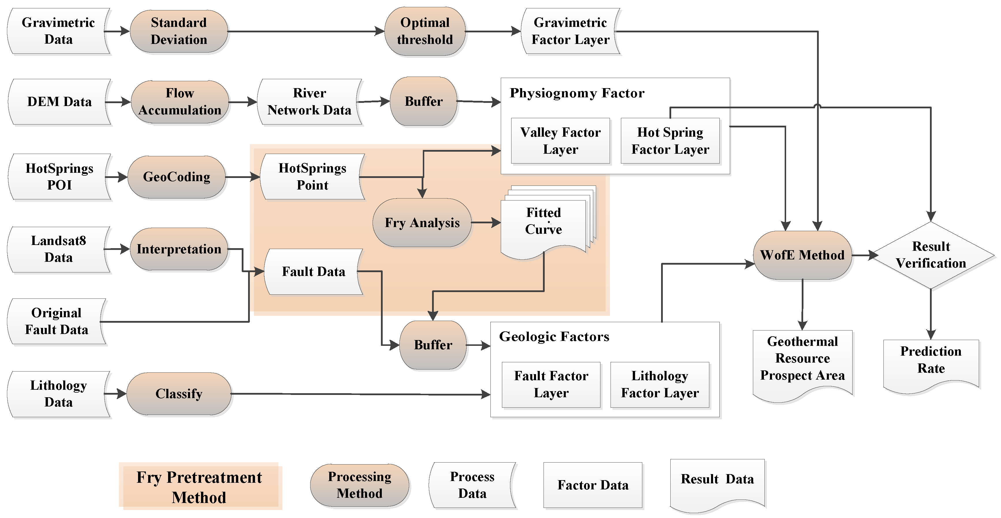
In this study, the workflow of the Fry-WofE geothermal resources forecast is shown in Figure 2. The core contents of the Fry-WofE workflow include the following points:
- Preliminary data processing includes geocoding the hot spring points, extracting data from DEM (digital elevation model), doing STD (standard deviations) according to the gravity anomaly data, using remote sensing to enrich the existing fault, and classifying the geological layer that effects the hot spring distribution.
- Performing Fry analysis on the hot spring data and the curve fitting of the relationship between the trend direction and the quantity of hot springs will be done after analysis. Then the weight of fault data will be calculated according to the fit of the curve after subdivision. At last, the weighting result will be used to determine the parameters for buffer analysis. We finally get the fault evidence layers.
- Complete the WofE calculation for each evidence layer and get the prediction result.
3.2. Data
The improvement of the fault treatment method is the main characteristic of the Fry-WofE method. The analysis of the fault factor shows special importance because the fault in the Liaoning region has a great influence on the development of geothermal energy. In this paper, ArcGIS (The best commercial GIS tool of the world) and SPSS (The first statistical analysis software of the world) tools are selected for spatial analysis and statistical analysis, and the preprocessing of original data needs to be done. Then we can get hot spring point data, river network data, lithologic data, Bouguer gravity data, and fault data after remote sensing interpretation processing.
The total number of hot springs in the study area is 33, among which 24 were obtained by digitizing historical data, three were found by field survey, and six is were obtained by searching the Internet. Among them, there are 28 artesian springs and five artificial mining hot springs.
The geological unit data we used comes from a 1:250,000 geological map, which was drawn by the Research Institute of Geology and a survey of the mineral resources of Liaoning province and Jilin Province, and it has been revised and supplemented by the project named “Deep geological survey of Linjiang and Benxi” by the China Geological Survey.
This study uses four Landsat8 remote sensing images; the map numbers are LC81180312016090LGN00, LC81180322014276LGN00, LC81180312016138LGN00, and LC81190322016241LGN00. They are suitable for visual interpretation as they have less cloud cover and false color composition (red-green-blue false color: 752) is adopted to improve the recognition of surface features. The interpretation results are classified into fracture data after comparison with a geological map.
The application of a digital elevation model (DEM) is increasingly extensive (I. D. Moore, 1991). The DEM data used in this study is ASTER GDEM (global digital elevation model) data, the mesh accuracy of which is 30 m and the elevation accuracy of which is 7 m. Valley data are derived from DEM data after hydrological treatment. The vector data of the river network have been obtained after filling and analyzing the flow direction with the DEM data, computing flow accumulation data, and extracting the grid and vectorization. The two data sets above are provided by the Geospatial Data Cloud site of the Computer Network Information Center at the Chinese Academy of Sciences (http://www.gscloud.cn).
3.3. The Fry-WofE Method
Fry-WofE is based on the WofE method, a data driven model. Before forecasting the prediction probability, the predicted target number or target area should be calculated. When the probability of evidence factors and the prediction appear at the same time, the predicted goal they control will be more important and more accurate. The weighted value of the corresponding weight factor will be larger at the same time. Each weight factor, which is an evidence layer, is superimposed and covered. The expectation map of different levels can be obtained by weighted overlay and coverage synthesis by using the statistical evidence of each grid layer as the prediction target.
Before the calculation of the weights of the evidence model, we should deal with the weight of the layer that will be calculated for binarization. Let the map range equal S, the cell size of the layer be s, and the abnormal value that indicates this be P (the P range is not completely coincident with the actual point set Q of the geothermal anomaly). At this time, the prior probability of the layer is O(P), indicating the probability of a geothermal anomaly occurring in the position region. The weight of each layer is calculated respectively, and finally the comprehensive predictive factor map is obtained under the influence of many layers, the weighted evidence of which is computed by the prior probability of each layer.
According to the traditional evidence weighting model:

The prior probability is:
The weight of evidence is:
where indicates the significant extent of the geothermal anomaly at the i section in the evidence layer. The formula is shown as follows:
In the Fry-WofE method, before the weighted calculation of the evidence (take fault layer L as an example), the parameters for the subdivision layer of the evidence layer should be split. The prior probability of the subdivision layer can be obtained by the Fry model statistics. The formula is as follows:
is the distribution frequency of the kth small fault in the Fry analysis rose diagram and n is the number of evidence points.
Then, , which can fit the fault distribution frequency, can be obtained using:
and type n should be satisfied:
The should be a small constant, ensuring that the normr value (comparing between and ) won’t change too much. They can converge to in the local scope.
In addition, The StudentC method is used to reflect the significance of the C value. The formula is as follows:
were the variance of , and C, respectively.
Finally, in the comprehensive analysis of the multivariate data uses the following to calculate the weight S of the n layers and the prediction results, respectively:
where is the C value of ith layer and is the S value of ith layer. Then the formula is normalized to make .
3.4. Hot Spring Data Processing by the Fry Method
Fry analysis, an analysis method first applied in petrology and the structural domain, was proposed by Fry in 1979. Fry analysis can indicate the direction of tectonic stress by locating spots and points and calculating their direction distribution, thus indicating the distribution direction of point or line objects. Later, many scholars expanded the scene of application to spatial distribution analysis [39,40] and achieved good results [6]. Fry analysis [41] can operate manually by using a sheet of tracing paper on which a series of parallel reference lines (typically north pointing on a map) have been drawn and the location of each data point is recorded. On a second sheet of tracing paper with a center point (or origin), a set of marked parallel lines are kept parallel to those on the first sheet. The origin of the second sheet is placed on one of the data points on the first sheet, and the second sheet is marked with all the positions of points on the first. Then the origin of the second sheet is placed on a different data point on the first, and the positions are again recorded on the second sheet. This is continued, maintaining the same orientation, until all the points on the first sheet have been used as the origin on the second. For n data points, there are n2 − n translations. The resulting Fry plot may be further analyzed by the construction of a rose diagram, recording join frequency versus directional sector. The Fry method provides a better visualization of spatial distribution by redrawing the distribution features that are not visible.
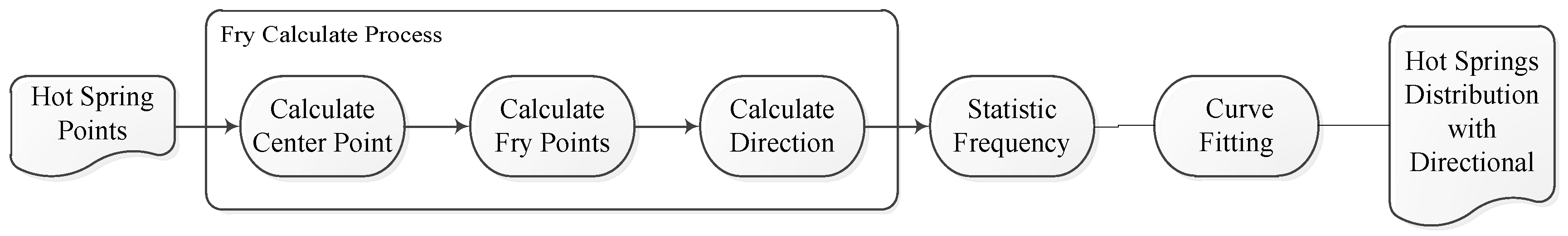
The spatial distribution of hot springs is the reasoning premise of the reverse inference of the extent of the influence of fault lines. Fry analysis [41] has appeared in scholars’ studies like those by Noorollahi, Moghaddam, and Wibowo [2,3,4], but it was used only to show the distribution trend of objects or as an auxiliary tool for spatial analysis. Since the distribution of hot springs can be determined by the Fry angle rose diagram, the distribution trend of hot springs can also be expressed by the Fry method. The fault consistent with this trend should be given higher weight in later calculations. In this study, the process of applying Fry analysis to hot spring data is shown in Figure 3.
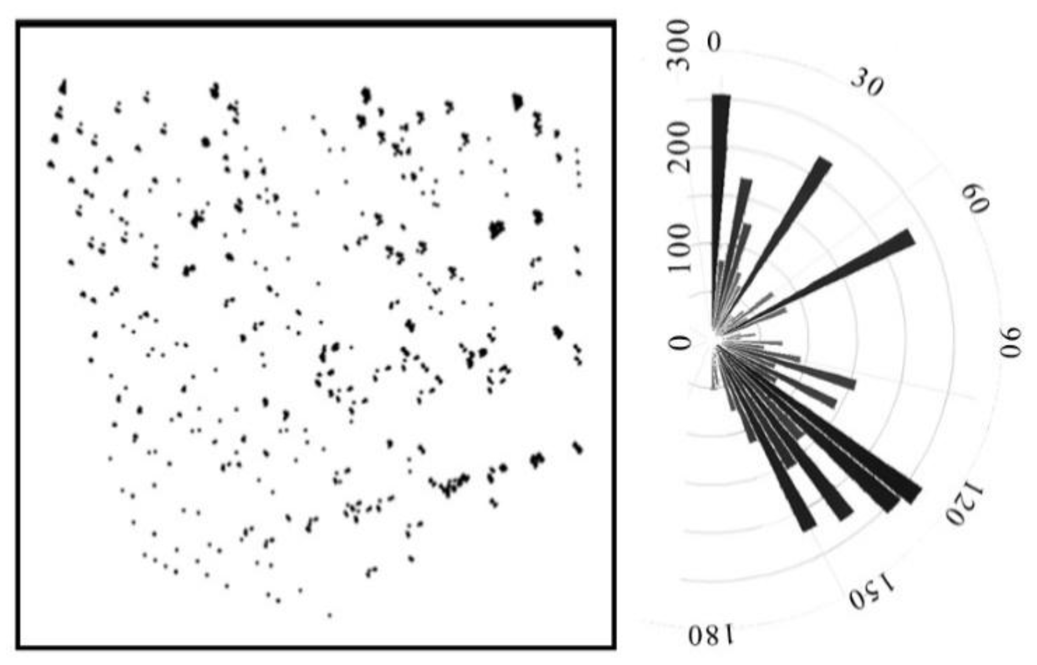
After repeated drawing of the hot springs in the study area by the Fry method, the spatial distribution results are shown as follows. The orientation of the Fry points is concentrated from 120° to 160° and 0° (Figure 4). It shows that the distribution of hot spring points in eastern Liaoning province is obviously NW and NS trending. This is consistent with studies of our predecessors, which have considered the hot springs to be mainly distributed on both sides of faults in the NW and nearly NNE directions [24,42].
The geographical data is discrete but also continuous [43]. The frequency distribution of faults in all directions is discontinuous. In order to make the different orientations of faults smooth and reduce the ‘cliff intermittent’ of the forecast results, we should use a curve fitting method to fit the Fry points distribution data. In this study, high order curve fitting is adopted, in which the number of fitting numbers is determined by the Fry number and the residual maximum modulus and the degree of discretization of the angular data is reduced by polynomial fitting.
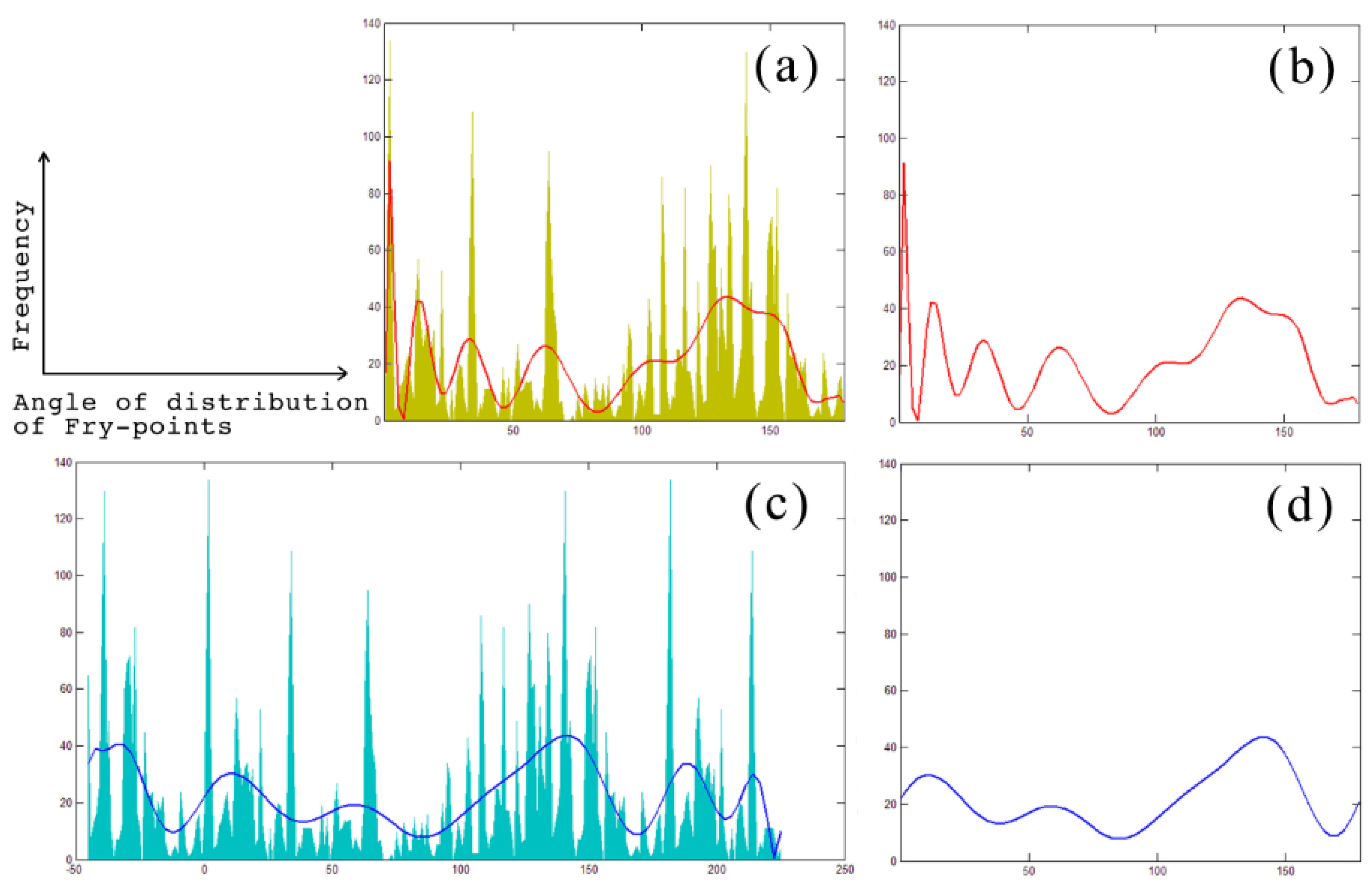
Figure 5a,c is the Cartesian coordinate graph, which plots frequency on the vertical Y-axis against the angle of distribution of the Fry-points on the horizontal x-axis, including orientations from 0° to 359°, where 0° to −179° and 180° to −359° are repeated; we can only adjust for the 0° to −179° range. In order to ensure the fitting accuracy of the two curves, the data should be processed at both ends before fitting the curve. The amount of data in the range of the augmented existing data in two segments of the quarter has a distribution angle of 45°. The fitting range expanded from −45° to −225° to ensure a fitting accuracy between 0° to −179°, making the curve equal the values from 0° to 180°. Figure 5 shows examples of cases of high-order curve fitting by 20 times. Compared with the original method of Figure 5b fitting Figure 5a, the method of Figure 5d fitting Figure 5c can obviously obtain better processing results at both ends of the fitting curve without changing the amount of data.
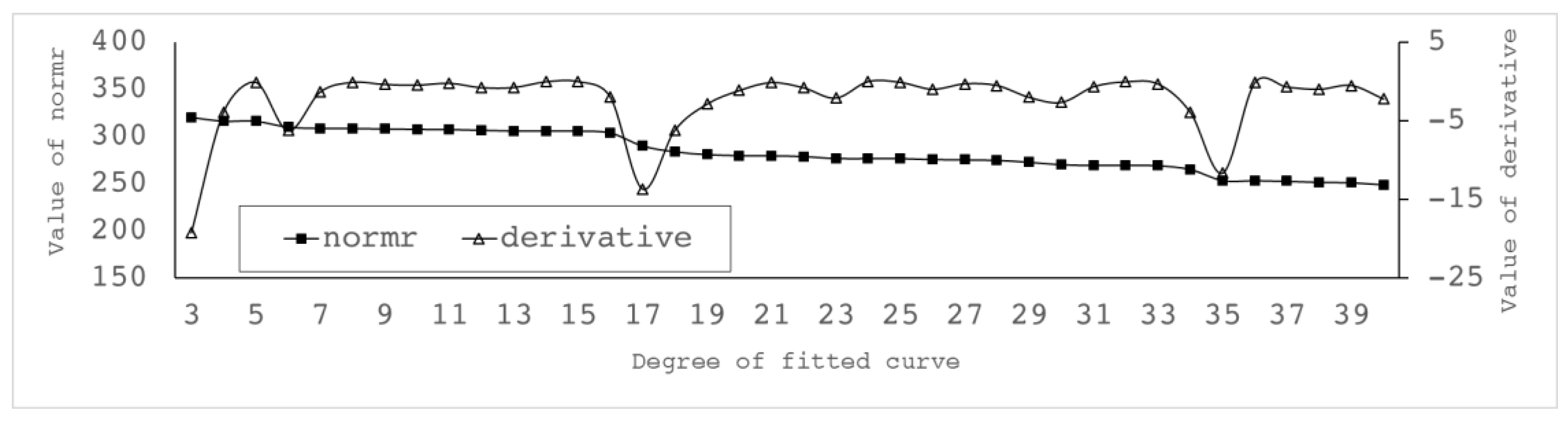
In order to evaluate the effect of curve fitting and determine time of the best fitting curve, the normr value is introduced as the evaluation criterion, and normr is the maximum modulus of the residual. The smaller the value, the better the fitting accuracy of the curve. In the curve fitting of Fry distribution data, if the time of the fitting curve equation is too high, it is easy to over fit. If it is too low, it cannot accurately fit the distribution. There are 33 data points of hot spring spots in this region. The number time of fitting curve equation, n, should be within 3–33, and n should make the normr value of the curve as small as possible or make the normr value change less obviously at n. By comparing the normr values of the three to 33 curves (Figure 6), it can be seen that the normr values change little from 20 to 33, that they have almost converged, and that the values are lower than the normr values from three to 19. As you can see from the diagram, n = 20 is at the earliest stable position after the change of the slope of the curve. Therefore, this experiment chooses 20 as the best parameter of the fitting curve.
In order to establish the relationship between the fitting curve and the weight, we put the fitting curve of the normalized y values in the range of 0 to 1. We use MatLab, letting x = 0:0.01:180 from 0 to 180, with 0.01 for each step for the fitting results, to find the lowest and highest point of the function curve through the transformation:
This is used to find the fitting function equation after normalization. The 20th curve equation used in this study is:
x is the fault orientation, and z is the intermediate value for centering and scaling the x value. The values of to are shown in Table 1.
We establish the relation between the fault orientation and the frequency distribution of the hot spring by fitting the curve, yet the distribution frequency of hot springs is positively related to the spatial distribution of hot springs. Thus, the relationship between the fault orientation and the geothermal distribution trend has been established.
In order to reduce fracture data discontinuities caused by too few data at the reflection points, it is necessary to smooth the fault data without affecting the accuracy, and, after smoothing, the corners become denser. It is convenient to segment the fault data into a large number of small faults and then to obtain the orientation of each minor fault. Combined with the fitting curve obtained before, the buffer distance of the fracture under the orientation weighting correction is obtained.
The λ is the parameter to be determined. We need to use the weights of evidence method to determine its optimum value.
The accuracy of the DEM data used in this study is 90 m, so the buffer step of fault data we used in WofE processing is less than 90 m, which is enough to meet the precision requirements. Experiments show that, when the threshold value is up to 700 m, the buffer area has completely covered all the authentication points. Continuing to increase the threshold does nothing to support the weight of the evidence. Therefore, we take the threshold from 40–2000 m, with 70 m steps into the buffer calculation. The corresponding buffer area is calculated from 474 km2 to 16,327 km2, and the weight of the evidence is calculated in the attached table (Table A1).
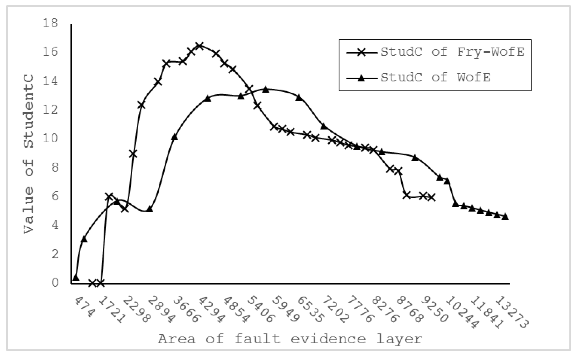
When the fault layer is treated as the evidence layer by the Fry method, the buffer distance of the fault is determined by λ. It can be calculated by Formula 12; when λ has avalue from 5 to 35, it can make the fault buffer area correspond from 1432 km2 to 9487 km2 (Table A2). It is convenient to compare the effect of the fault layer with the Fry-WofE and WofE methods (Figure 7). We placed StudC (student C index that the response of the data) and the area of calculation result in one graph, and we can found that the fault layer after Fry analysis in the evidence weighted calculation process has a better StudC response (Figure 8).
3.5. Calculation of the WofE Layer
3.5.1. Weight Evidence Calculation of River Network Layer
Water is an ideal medium for heat exchange. In the eastern Liaoning Province, the existence of water is a necessary condition for the development of geothermal fields and hot springs. The river network is also an important factor. The river valleys provide sufficient water and water head pressure for the surrounding hot springs.
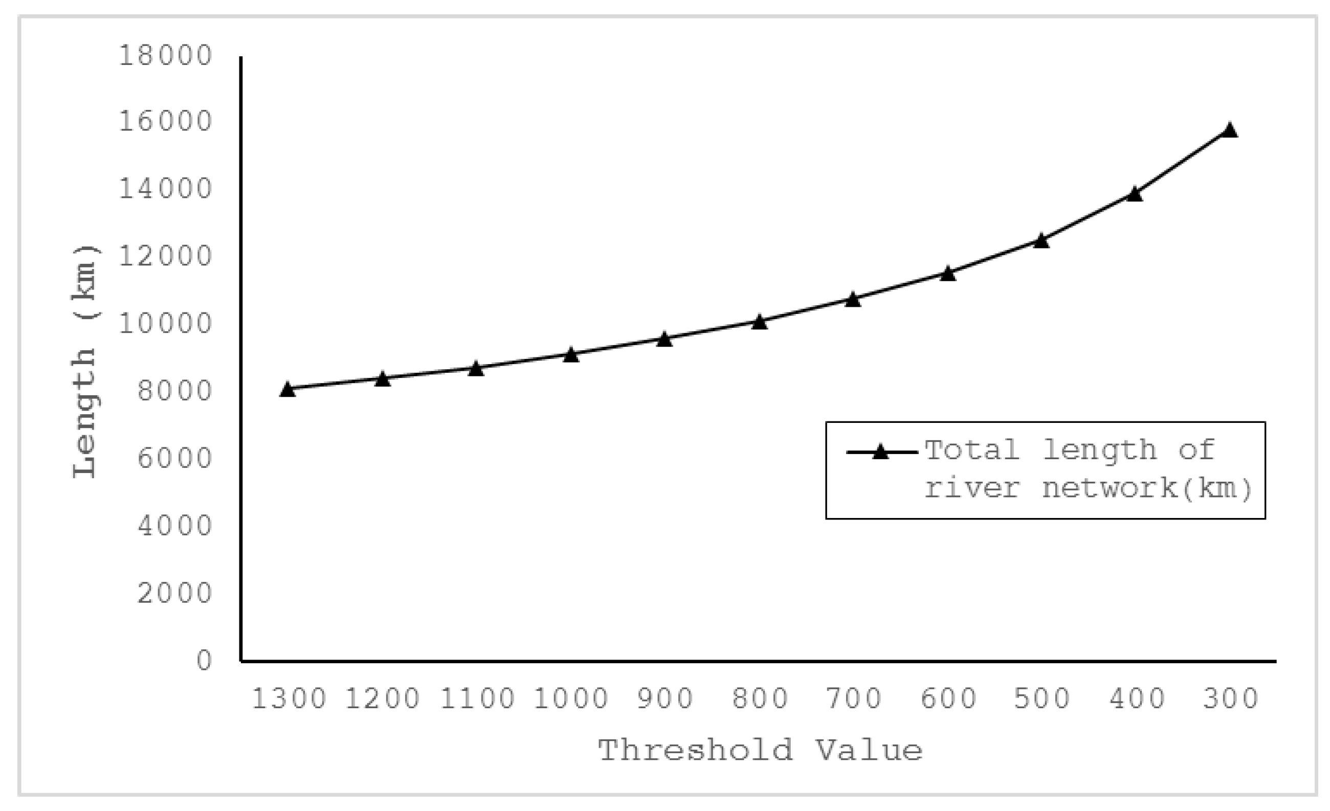
The river network grid in this study is determined to ahave 800 units, according to the principle; ‘the turning point where the river length changes from short to long [44]. In the present study, the extraction threshold was determined to be 800 (Figure 9). It is only from the low elevation lines in each cell of the DEM that the river network data it extracted (Figure 10a). In order to show the impact of the river valley, we need to establish a buffer zone by using spatial analysis. The buffer distance in the river network buffer is selected to be from 50 m to 1 km to calculate respective evidence weights. Finally, according to the StudC value, 350 m is determined as the optimum parameter for the river network buffer (Table A3).
3.5.2. Weight Evidence Calculation of Lithologic Layer
There are two main influences of lithologies on geothermal energy. On the one hand, faults and fractures in different lithological distribution areas have different developmental characteristics. On the other hand, the radioactive thermal effect of granite is an important factor that affects geothermal development; 57% of the known hot springs in the study area developed in Mesozoic granite bodies (Figure 10b).
According to the research of the geological data and the position of exposed hot springs in eastern Liaoning Province, we selected four categories that have broad representation and distribution of rock types in study area, including Late Triassic and Early Cretaceous intrusive rocks, Late Archean granite, and the Yangshugou and Gaixian groups in the Liaohe group of Proterozoi. Then, the weights of four types of lithology and geothermal anomaly points are calculated (Table A4).
3.5.3. Weight Evidence Calculation of Bouguer Gravity Anomaly
The Bouguer gravity data reflects the change information in different densities of underground geological bodies. In the area, the distribution of hot springs has obvious relation with the gradient of the gravity anomaly zone, which is usually a reflection of a fault or geological boundary. In order to highlight the anomalies of gravity and the distribution of gradient bands, this study uses an 8 × 8 grid window to extract standard deviations (STD), that is, to reflect the extent of gravity anomalies within the 4 × 4 km rectangle in the region [45]. The higher the value of the Bouguer gravity anomaly difference, the higher the STD value. In this study, we use the method of fixing the maximum value and constantly adjusting the minimum value to find the interval optimal solution of the gravity anomaly STD for points evidence of the hot springs (Figure 10c). With 0.2 units as a step, the total is divided into 17 intervals; for example, we set the first interval of the range of values of the gravity anomaly value STD corresponding to the 6.3–6.1 and the second to 6.3–5.9. Then we calculated respectively the weight of each evidence layer value for the STD gravity anomaly distribution map and the STD interval and evidence weight value correlation table (Table A5).
4. Prediction and Comparison of WofE and Fry-WofE Methods
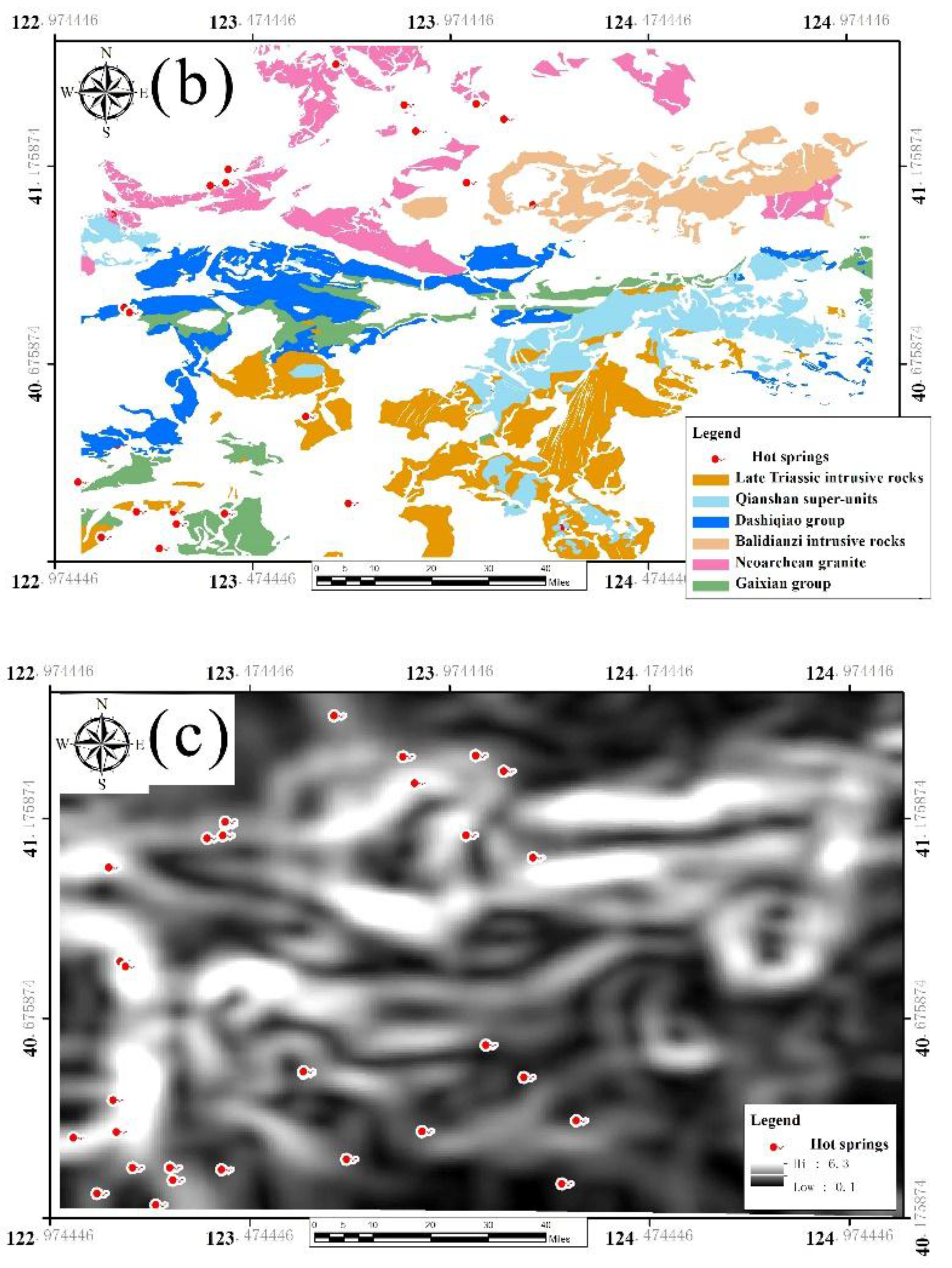
In the region where the geothermal field develops, if spring water comes into contact with a heat source during its cycle process, the temperature rises and outcrops to the surface, then there is a hot spring. Therefore, hot spring points can be used to verify the rationality of geothermal region prediction. In this study, the geothermal potential evaluation layer is obtained by analyzing and normalizing the weighted layers area. Based on past experience, we selected 10%, 20%,and 80% of the total area as a prospective division threshold. The top 10% of the area potential value is selected as the high potential area of the prediction model, and 10% to 20% is the middle potential area (Figure 11).
In order to compare the prediction ability and the accuracy of the two methods, all the data points were used as the validation data to compare the statistical results of the two methods (Table 2). In the high prediction area, the validation point hit by the Fry-WofE method reached 18, yet validation point of the WofE method was 12. In the middle prediction potential area, the validation point hit by Fry-WofE method was 6, while that of the WofE method was 8.
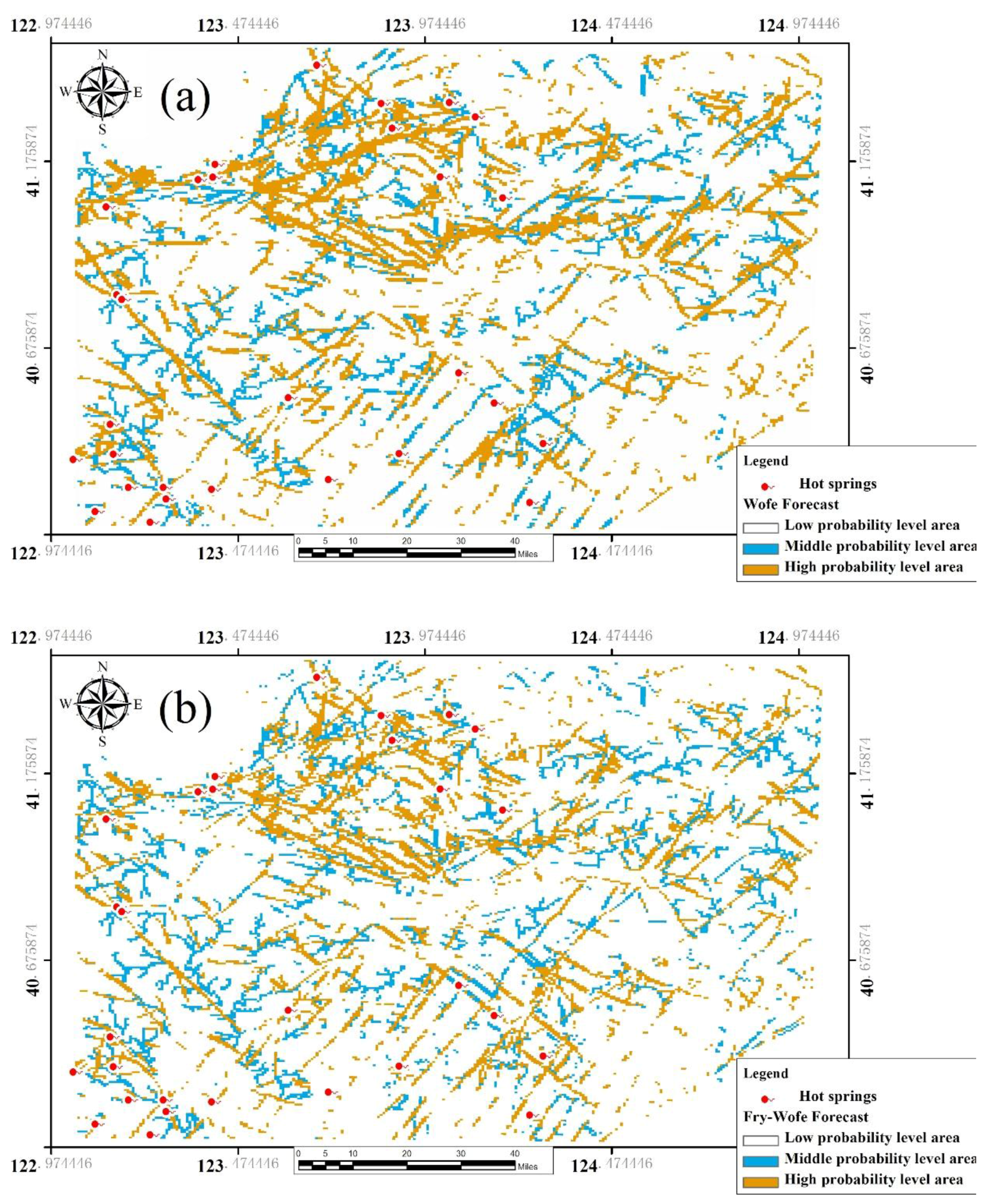
We normalize the prediction results of the two methods, then use the Fry-WofE result minus the WofE result to obtain a prediction difference map in Figure 12. Each grid value in the diagram represents the difference between the predicted results of the Fry-WofE method and the WofE method. The red part of the diagram is the area in which the predictive verification of the Fry-WofE method is higher than the WofE method, and the blue part is the area in which the predictive verification of Fry-WofE method is lower than the WofE method. As we can see, there are more hot springs in the red area, only a few hot springs in the green area (Figure 12a,c, and only one hot spring point is distributed in the blue area (Figure 12b region). Figure 12 shows that the Fry-WofE method is better than the traditional WofE method in fitting the existing hot spring points.
The distribution of geothermal resources has high control over fractures, as can be seen from the prediction results; the weight of the fault data is much higher than that of the other data mentioned in the model calculation. The traditional WofE method without pretreatment has the same effect on the results of faults at different angles, with lower responses than the results of the Fry-WofE method in the NW direction region, in which the hot springs aremainly distributed, and higher responses in other invalid areas. The Fry-WofE method gives different weights by the attributes of the fault layers, which makes the prediction more accurate under the background that the results are obviously controlled by fewer factors.
5. Conclusions and Discussion
5.1. Advantages of the Fry-WofE Method
From the evidence layer calculation process of fracture data, the Fry-WofE method can get better prediction results than WofE and cover more hot spring points (Figure 12) with less area (Figure 8). As can be seen from the experiments, the Fry-WofE method has a higher predictive power than the WofE method, that of the former being 12.1%. It proves that the Fry-WofE method is a more accurate and effective prediction method. Especially when the distribution of anomalies in the study area is directional, the Fry-WofE method can give better prediction results.
5.2. Geothermal Resources and the Prospect of Hot Springs
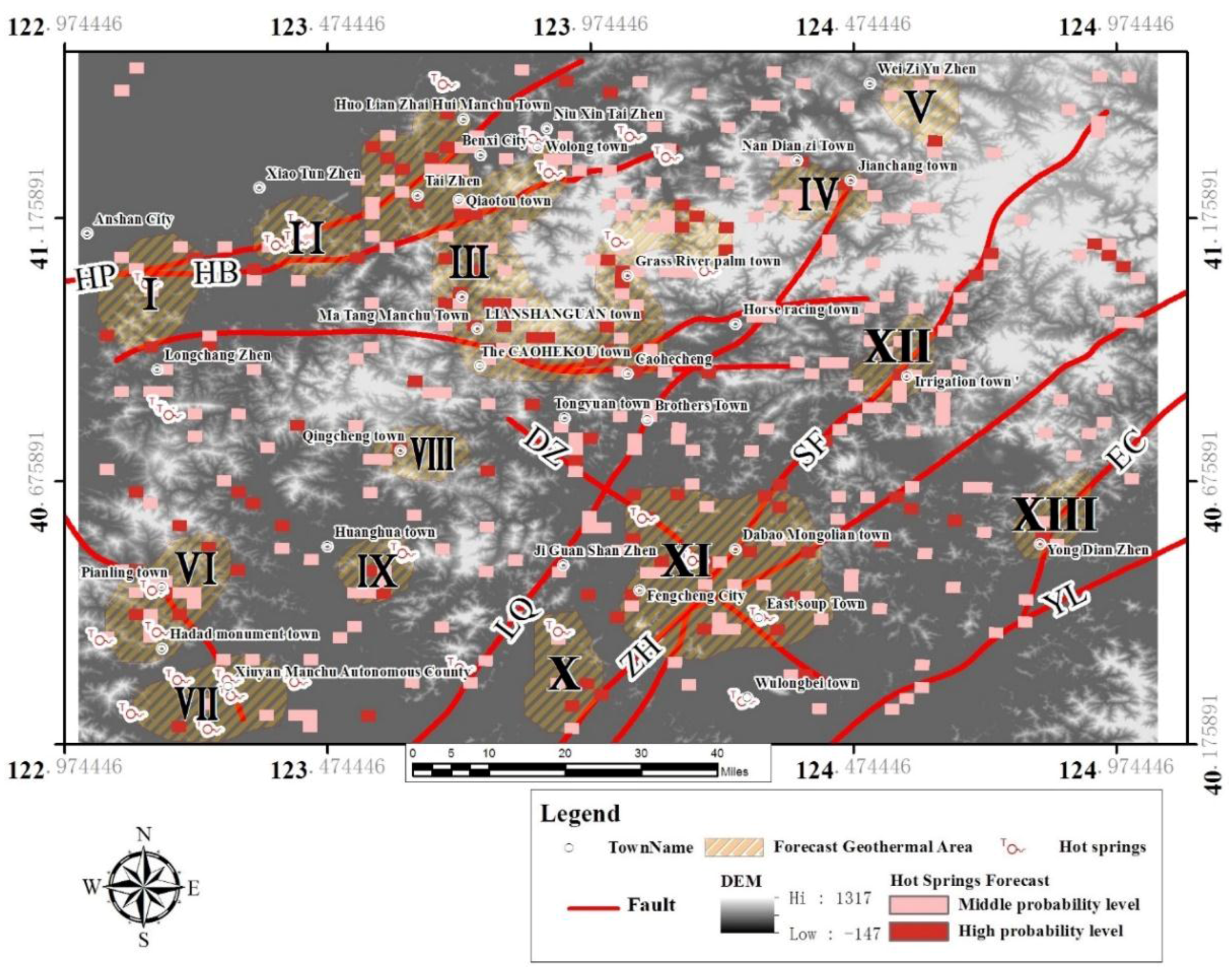
Geothermal development is a necessary but not sufficient condition to produce hot springs, and topography (water head pressure) is another important condition that influences the emergence of hot springs. We extract the intersection of Fry-WofE forecast results and river buffer data to obtain the prospective distribution area of hot springs in the study area. We superimposed the high potential and median potential area of the predicted results with river valley data, then obtained the forecast area of hot springs in eastern Liaoning Province. In Figure 13, they are red and pink, respectively.
A number of geothermal prospective areas have been planned, as can be seen in Figure 13. These geothermal prospective areas mainly include areas alongside the Hanling-pianling fault (HP) and Hanling-benxi (HB); the confluence of the Caohekou part and the Lianshanguan extended area of the Hanling-caohecheng fault (HC) and the Sipingjie-fengcheng fault (SF); the confluence of the Zhuanghe-huanren fault (ZH), Sipingjie-fengcheng fault (SF), and Daheishan-zhangjiapu fault (DZ); and areas alongside the Haicheng-xiuyan fault (HX). There are geothermal prospect responses at the Yongdian part of the Erpengdianzi-changdian fault (EC), Qingchengzi, eastern Weiziyu, Jianchang, and Huanghuadia. We have planned 13 prospective areas, but the newly discovered geothermal prospective areas, including IV, V, VI, XII, and XIII, have not exposed hot springs and geothermal resources yet. Thus, there is great potential for development in the future.
5.3. Discussion
The distribution of geothermal resources in eastern Liaoning Province is not obvious except for fault control, so most of the evidence factors affecting geothermal resource distribution are concentrated in fault layers. The traditional WofE method does not take into account the influence of directional attributes on the distribution of geothermal resources when dealing with the evidence layer. Therefore, the result of examining the XI geothermal prospective area, which is mainly NW distributed, with the Fry-WofE prediction method is better than that with the WofE method. Similarly, in the northern part of the III region, the WofE method is also less accurate than the Fry-WofE method. The posterior probability of the existing verification points is generally low, which is the main reason for the unsatisfactory prediction results of the WofE method in the geothermal prediction research into fault control.
If there is no further processing for the fault data, as a buffer zone for all fracture parameters within fracture control will be unified. A large area will be also buffered in garbage areas where the fault is controlled but the hot springs are not apparent. In these garbage areas, the areas are counterproductive to the weight of the evidence. According to the WofE method, using a smaller area to cover more of the verification points can make the weight of the evidence value of the layer higher. The Fry-WofE method uses the Fry method to locate the orientation influence on the fault and reduce the garbage buffer area size by setting buffer parameters according to the fault orientation weight, which can significantly enhance the accuracy of the prediction results.
Using the Fry method for fault weighting preprocessing in this case, from this perspective, is only one option. The Fry method can only compute the weight of the fault path orientation, but many data features are multidimensional or even high-dimensional. For example, a fault has fault properties, tendencies, fault throw, forming times, and other attributes. Much work remains to be done on how to find suitable preprocessing methods for different attributes of different data. Multivariate data often does not have a unified dimension, and its attributes do not have a unified dimension either. The relationship between attributes is a lack of correlation with demonstration, and the existing dimensionality reduction algorithms cannot be used directly. However, how to define and quantify these attributes remains a problem because the influence of each attribute and their weighting in different cases are different. At present, in the process of processing surface features, spot features, or three-dimensional geologic bodies, introducing appropriate methods to process data can play a very positive role in the results of the WofE model, which should be especially true when subjects are under the control of a small amount of evidence.
5.4. Conclusions
- When the distribution of the geothermal resources is obviously influenced by the geological factors of fault orientation, the Fry-WofE method can take into account the influence direction of geological factors on the prediction results to obtain more accurate forecast results.
- 13 geothermal prospective areas were predicted by the Fry-WofE method in eastern Liaoning Province, which provided reference data for further geothermal exploration and development in this area.
Acknowledgments
The project was completed under the auspices of National Key R & D Program of China (2016YFC0803109, 2016YFB0502605) and China Geological Survey Project “Deep geological investigation project of Benxi Linjiang area (1212011220247)”.
Author Contributions
Linfu Xue and Xuejia Sang conceived and designed the experiments; Jiwen Liu perfected English writing; Liang Zhan contributed analysis tools; Xuejia Sang analyzed the data and wrote the paper.
Conflicts of Interest
The authors declare no conflict of interest.
Appendix A

Table A1.
Weight of evidence of the fault calculated with the WofE method.
| Buffer Distance (m) | W+ | W− | C | W+2 | W−2 | C2 | StudC | |
|---|---|---|---|---|---|---|---|---|
| Weight of evidence of fault about WofE method | 40 | 0.44 | −0.01 | 0.45 | 1.00 | 0.03 | 1.03 | 0.44 |
| 110 | 0.82 | −0.07 | 0.89 | 0.25 | 0.03 | 0.29 | 3.13 | |
| 180 | 0.89 | −0.15 | 1.04 | 0.14 | 0.04 | 0.18 | 5.73 | |
| 250 | 0.71 | −0.15 | 0.86 | 0.13 | 0.04 | 0.17 | 5.20 | |
| 320 | 0.96 | −0.34 | 1.30 | 0.08 | 0.05 | 0.13 | 10.18 | |
| 390 | 1.04 | −0.52 | 1.56 | 0.06 | 0.06 | 0.12 | 12.86 | |
| 460 | 1.00 | −0.62 | 1.62 | 0.05 | 0.07 | 0.12 | 13.02 | |
| 530 | 1.02 | −0.82 | 1.84 | 0.05 | 0.09 | 0.14 | 13.47 | |
| 600 | 1.03 | −1.10 | 2.14 | 0.04 | 0.13 | 0.17 | 12.94 | |
| 670 | 1.05 | −1.53 | 2.59 | 0.04 | 0.20 | 0.24 | 10.96 |
Wi(k) is the weight for the k-th class value of the i-th evidential theme and reflects the degree of spatial association of the known deposits with that class value. For binary themes, W(1) and W(0) are usually labelled W+ and W−, respectively for presence or absence. The C (contrast) for an evidential theme is defined as the range of the weights, or Wmax-Wmin over all classes, or W+-W− if the theme is binary. And StudC (Student C) index that the response of the data.
Table A2.
Weight of evidence of the fault calculated with the Fry-WofE method.
| W+ | W− | C | W+2 | W−2 | C2 | StudC | ||
|---|---|---|---|---|---|---|---|---|
| Weight of evidence of fault about Fry-WofE method | 7 | 0.94 | −0.15 | 1.09 | 0.14 | 0.04 | 0.18 | 6.01 |
| 8 | 0.81 | −0.14 | 0.95 | 0.14 | 0.04 | 0.18 | 5.20 | |
| 9 | 1.04 | −0.25 | 1.29 | 0.10 | 0.04 | 0.14 | 8.99 | |
| 10 | 1.20 | −0.37 | 1.58 | 0.08 | 0.05 | 0.13 | 12.38 | |
| 11 | 1.25 | −0.47 | 1.72 | 0.07 | 0.06 | 0.12 | 14.01 | |
| 12 | 1.29 | −0.57 | 1.86 | 0.06 | 0.06 | 0.12 | 15.29 | |
| 13 | 1.27 | −0.62 | 1.89 | 0.06 | 0.07 | 0.12 | 15.41 | |
| 14 | 1.30 | −0.75 | 2.05 | 0.05 | 0.08 | 0.13 | 16.11 | |
| 15 | 1.37 | −1.00 | 2.37 | 0.04 | 0.10 | 0.14 | 16.48 | |
| 16 | 1.35 | −1.09 | 2.44 | 0.04 | 0.11 | 0.15 | 15.94 | |
| 17 | 1.33 | −1.19 | 2.53 | 0.04 | 0.13 | 0.17 | 15.28 | |
| 18 | 1.28 | −1.18 | 2.46 | 0.04 | 0.13 | 0.17 | 14.86 | |
| 19 | 1.30 | −1.45 | 2.75 | 0.04 | 0.17 | 0.20 | 13.50 | |
| 20 | 1.29 | −1.62 | 2.91 | 0.04 | 0.20 | 0.24 | 12.33 | |
| 21 | 1.28 | −1.83 | 3.11 | 0.03 | 0.25 | 0.28 | 10.91 | |
| 22 | 1.23 | −1.81 | 3.05 | 0.03 | 0.25 | 0.28 | 10.70 | |
| 23 | 1.19 | −1.80 | 2.99 | 0.03 | 0.25 | 0.28 | 10.50 | |
| 24 | 1.15 | −1.78 | 2.94 | 0.03 | 0.25 | 0.28 | 10.31 |
Table A3.
Weight of evidence of the river network.
| Buffer Distance (m) | W+ | W− | C | W+2 | W−2 | C2 | StudC | |
|---|---|---|---|---|---|---|---|---|
| Weight of evidence of river network | 50 | 1.37 | −0.10 | 1.47 | 0.25 | 0.03 | 0.29 | 5.13 |
| 100 | 1.37 | −0.21 | 1.59 | 0.13 | 0.04 | 0.17 | 9.59 | |
| 150 | 1.09 | −0.22 | 1.32 | 0.11 | 0.04 | 0.15 | 8.59 | |
| 200 | 1.01 | −0.28 | 1.29 | 0.09 | 0.05 | 0.14 | 9.43 | |
| 250 | 0.96 | −0.34 | 1.30 | 0.08 | 0.05 | 0.13 | 10.23 | |
| 300 | 0.86 | −0.35 | 1.22 | 0.07 | 0.05 | 0.12 | 9.79 | |
| 350 | 0.91 | −0.49 | 1.40 | 0.06 | 0.06 | 0.12 | 11.52 | |
| 400 | 0.78 | −0.46 | 1.24 | 0.06 | 0.06 | 0.12 | 10.19 | |
| 450 | 0.73 | −0.48 | 1.21 | 0.06 | 0.07 | 0.12 | 9.91 | |
| 500 | 0.69 | −0.52 | 1.20 | 0.05 | 0.07 | 0.12 | 9.67 | |
| 550 | 0.70 | −0.63 | 1.33 | 0.05 | 0.08 | 0.13 | 10.15 | |
| 600 | 0.22 | −1.41 | 1.63 | 0.03 | 0.50 | 0.53 | 3.05 | |
| 650 | 0.62 | −0.59 | 1.21 | 0.05 | 0.08 | 0.13 | 9.25 | |
| 700 | 0.15 | −1.71 | 1.87 | 0.03 | 1.00 | 1.03 | 1.81 | |
| 750 | 0.55 | −0.55 | 1.10 | 0.05 | 0.08 | 0.13 | 8.39 | |
| 800 | 0.53 | −0.60 | 1.13 | 0.05 | 0.09 | 0.14 | 8.26 | |
| 850 | 0.51 | −0.65 | 1.16 | 0.04 | 0.10 | 0.14 | 8.11 | |
| 900 | 0.50 | −0.72 | 1.21 | 0.04 | 0.11 | 0.15 | 7.93 | |
| 950 | 0.49 | −0.79 | 1.28 | 0.04 | 0.13 | 0.17 | 7.72 | |
| 1000 | 0.48 | −0.88 | 1.35 | 0.04 | 0.14 | 0.18 | 7.46 |
Table A4.
Weight of evidence of Lithology.
| Lithology | W+ | W− | C | W+2 | W−2 | C2 | StudC | |
|---|---|---|---|---|---|---|---|---|
| Weight of evidence of Lithology | Late Triassic epoch intrusive rocks | 1.267 | −0.228 | 1.495 | 0.201 | 0.071 | 0.272 | 5.497 |
| Early Cretaceous intrusive rocks | 0.690 | −0.089 | 0.779 | 0.334 | 0.063 | 0.396 | 1.965 | |
| Gaixian and Yangshugou group | 0.193 | −0.020 | 0.213 | 0.500 | 0.059 | 0.559 | 0.381 | |
| The late Archean intrusive rocks | 1.243 | −0.125 | 1.369 | 0.334 | 0.063 | 0.397 | 3.449 |
Table A5.
Weight of evidence of Bouguer gravity anomaly STD.
| Bouguer Gravity Anomaly STD | W+ | W− | C | W+2 | W−2 | C2 | StudC | |
|---|---|---|---|---|---|---|---|---|
| Weight of evidence of Bouguer gravity anomaly STD | 6.3 > r > 4.0 | 0.709 | −0.058 | 0.767 | 0.708 | 0.243 | 0.748 | 1.025 |
| 6.3 > r > 3.8 | 0.842 | −0.101 | 0.943 | 0.578 | 0.250 | 0.630 | 1.498 | |
| 6.3 > r > 3.6 | 0.908 | −0.148 | 1.056 | 0.501 | 0.258 | 0.563 | 1.875 | |
| 6.3 > r > 3.4 | 0.686 | −0.124 | 0.810 | 0.500 | 0.258 | 0.563 | 1.439 | |
| 6.3 > r > 3.2 | 0.475 | −0.096 | 0.571 | 0.500 | 0.258 | 0.563 | 1.013 | |
| 6.3 > r > 3.0 | 0.263 | −0.060 | 0.323 | 0.500 | 0.258 | 0.563 | 0.574 | |
| 6.3 > r > 2.8 | 0.043 | −0.011 | 0.055 | 0.500 | 0.258 | 0.563 | 0.097 | |
| 6.3 > r > 2.6 | 0.069 | −0.023 | 0.092 | 0.447 | 0.267 | 0.521 | 0.177 | |
| 6.3 > r > 2.4 | 0.345 | −0.193 | 0.538 | 0.354 | 0.302 | 0.465 | 1.156 | |
| 6.3 > r > 2.2 | 0.391 | −0.307 | 0.698 | 0.316 | 0.333 | 0.460 | 1.518 | |
| 6.3 > r > 2.0 | 0.330 | −0.327 | 0.657 | 0.302 | 0.354 | 0.465 | 1.413 | |
| 6.3 > r > 1.8 | 0.284 | −0.353 | 0.637 | 0.289 | 0.378 | 0.476 | 1.339 | |
| 6.3 > r > 1.6 | 0.239 | −0.378 | 0.617 | 0.278 | 0.408 | 0.494 | 1.249 | |
| 6.3 > r > 1.4 | 0.183 | −0.383 | 0.566 | 0.267 | 0.447 | 0.521 | 1.086 | |
| 6.3 > r > 1.2 | 0.109 | −0.328 | 0.438 | 0.258 | 0.500 | 0.563 | 0.777 | |
| 6.3 > r > 1.0 | 0.107 | −0.622 | 0.729 | 0.243 | 0.707 | 0.748 | 0.975 | |
| 6.3 > r > 0.8 | 0.020 | −0.157 | 0.177 | 0.243 | 0.707 | 0.748 | 0.237 |
References
- Bellotti, F.; Capra, L.; Sarocchi, D.; D’Antonio, M. Geostatistics and multivariate analysis as a tool to characterize volcaniclastic deposits: Application to Nevado de Toluca volcano, Mexico. J. Volcanol. Geotherm. Res. 2010, 191, 117–128. [Google Scholar] [CrossRef]
- Noorollahi, Y.; Itoi, R.; Fujii, H.; Tanaka, T. GIS integration model for geothermal exploration and well siting. Geothermics 2008, 37, 107–131. [Google Scholar] [CrossRef]
- Moghaddam, M.K.; Samadzadegan, F.; Noorollahi, Y.; Sharifi, M.A.; Itoi, R. Spatial analysis and multi-criteria decision making for regional-scale geothermal favorability map. Geothermics 2014, 50, 189–201. [Google Scholar] [CrossRef]
- Wibowo, H.; Carranza, E.J.M.; Barritt, S.D. Spatial data analysis and integration in geothermal prospectivity mapping: A case study in West Java, Indonesia. In Proceedings of the 9th international symposium on mineral exploration (ISME IX), Bandung, Indonesia, 19–21 September 2006. [Google Scholar]
- Pradhan, B.; Oh, H.-J.; Buchroithner, M. Weights-of-evidence model applied to landslide susceptibility mapping in a tropical hilly area. Geomat. Nat. Hazard. Risk 2010, 1, 199–223. [Google Scholar] [CrossRef]
- Vearncombe, J.R.; Vearncombe, S. The spatial distribution of mineralization: Applications of Fry analysis. Econ. Geol. 1999, 94, 475–486. [Google Scholar] [CrossRef]
- Li, J. Prediction of geothermal resources in China based on evidence weighting method. J. Jilin Univ. 2012, 42, 7. [Google Scholar]
- Coolbaugh, M.F.; Zehner, R.E.; Raines, G.L.; Oppliger, G.L.; Kreemer, C. Regional Prediction of Geothermal Systems in the Great Basin, USA Using Weights of Evidence and Logistic Regression in a Geographic Information System (GIS). Available online: http://www.atlasgeoinc.com/wp-content/uploads/CoolbaughIAMGv10.pdf (accessed on 21 July 2017).
- Wang, D. Evaluation Method and Application of Mineral Resources Potential Based on SVM Model and Spatial Reasoning; University of Electronic Science and Technology of China: Chengdu, China, 2014. [Google Scholar]
- Zhao, J. Study on Comprehensive Evaluation of Mineral Resources (Gold Ore) in Typical Areas of Zhejiang Section; Zhejiang University: Hangzhou, China, 2015. [Google Scholar]
- He, B.; Wang, D.; Chen, C. A novel method for mineral prospectivity mapping integrating spatial-scene similarity and weights-of-evidence. Earth Sci. Inf. 2015, 8, 393–409. [Google Scholar] [CrossRef]
- Porwal, A.; Carranza, E.J.M.; Hale, M. A hybrid fuzzy weights-of-evidence model for mineral potential mapping. Nat. Resour. Res. 2006, 15, 1–14. [Google Scholar] [CrossRef]
- Ford, A.; Miller, J.M.; Mol, A.G. A comparative analysis of weights of evidence, evidential belief functions, and fuzzy logic for mineral potential mapping using incomplete data at the scale of investigation. Nat. Resour. Res. 2016, 25, 1–15. [Google Scholar] [CrossRef]
- Zhang, Z.J.; Zuo, R.G.; Xiong, Y.H. A comparative study of fuzzy weights of evidence and random forests for mapping mineral prospectivity for skarn-type Fe deposits in the southwestern Fujian metallogenic belt, China. Sci. China Earth Sci. 2016, 59, 556–572. [Google Scholar] [CrossRef]
- Mansour, Z.; Ali, P.; Mahdi, Z. A computational optimized extended model for mineral potential mapping based on WofE method. Am. J. Appl. Sci. 2009, 6, 200–203. [Google Scholar] [CrossRef]
- Cheng, Q.; Agterberg, F.P. Fuzzy weights of evidence method and its application in mineral potential mapping. Nat. Resour. Res. 1999, 8, 27–35. [Google Scholar] [CrossRef]
- Cheng, Q.; Zhang, S. Fuzzy Weights of evidence method implemented in GeoDAS GIS for information extraction and integration for prediction of point events. In Proceedings of the 2002 IEEE International Geoscience and Remote Sensing Symposium (IGARSS ’02), Toronto, ON, Canada, 24–28 June 2002; pp. 2933–2935. [Google Scholar]
- Cheng, Q.M.; Chen, Z.J. Application of fuzzy weights of evidence method in mineral resource assessment for gold in Zhenyuan district, Yunnan Province, China. Earth Sci. J. Chin. Univ. Geosci. 2007, 32, 175–184. [Google Scholar]
- Cheng, W.M. Enhancing the right of evidence (BoostWofE): The application of new methods in quantitative evaluation of mineral resources. J. Jilin Univ. 2012, 42, 1976–1985. [Google Scholar]
- Zuo, R.; Carranza, E.J.M. Support vector machine: A tool for mapping mineral prospectivity. Comput. Geosci. 2011, 37, 1967–1975. [Google Scholar] [CrossRef]
- Chen, W.; Chai, H.; Sun, X.; Wang, Q.; Ding, X.; Hong, H. A GIS-based comparative study of frequency ratio, statistical index and weights-of-evidence models in landslide susceptibility mapping. Arab. J. Geosci. 2016, 9, 204. [Google Scholar] [CrossRef]
- Zhang, G.; Cui, Y.; Yang, S.; Zuo, G. Distribution characteristics of underground hot water in Liaoning province. Investig. Sci. Technol. 2004, 2, 40–43. [Google Scholar]
- Liang, G. The thermal field of geological structure and reservoir condition analysis in Dandong Wulongbei. J. Dandong Teach. Coll. 1995, 3, 38–43. [Google Scholar]
- Zhou, S.; Xu, H.; Chen, X.; Yuan, J.F. Study on conceptual model of Tanggangzi geothermal system based on structural analysis in liaoning. Groundwater 2010, 32, 24–27. [Google Scholar]
- Zhang, Z. Underground water wulongbei hot spring two types of Liaoning. Geology 1985, 1985, 241–250. [Google Scholar]
- Tong, Z.; Cheng, S.; Li, W. Liaoning Province, Benxi Manchu Autonomous County caohezhang Zhen Tang Chi ditch geothermal anomaly analysis. Silicon Val. 2011, 2011, 156–168. [Google Scholar]
- Li, K.; Jin, S.; Yi, H.; Yue, C.; Yan, S. Benxi County Tangchi ditch thermal field thermal reservoir characteristics and the amount of resources. Liaoning Geol. 2000, 4, 304–308. [Google Scholar]
- Yousefi, H.; Noorollahi, Y.; Ehara, S.; Itoi, R.; Yousefi, A.; Fujimitsu, Y.; Nishijima, J.; Sasaki, K. Developing the geothermal resources map of Iran. Geothermics 2010, 39, 140–151. [Google Scholar] [CrossRef]
- Jeansoulin, R. Review of forty years of technological changes in geomatics toward the big data paradigm. ISPRS Int. J. GeoInf. 2016, 5, 155. [Google Scholar] [CrossRef]
- Energy Research Institute of Liaoning. Introduction of geothermal resources utilization in Liaoning province. Gas Heat 1984, 10, 61–64. [Google Scholar]
- Dongxiang, F.; Qi, W. Potential and countermeasures of exploitation and utilization of geothermal resources in Liaoning Province. Land Resour. 2008, S1, 98–99. [Google Scholar]
- Wang, X.K.; Qiu, S.W.; Song, C.C.; Kulakov, A.; Tashchi, S.; Myasnikov, E. Cenozoic volcanism and geothermal resources in Northeast China. Geol. Rev. 2001, 11, 150–154. [Google Scholar]
- Fang, R. Basic features of geological structure in Liaoning. Liaoning Geol. 1985, 3, 189–200. [Google Scholar]
- Liu, Y.; Yang, Z.; Li, S.; Xiang, L. The ancient Proterozoic extensional tectonic model—Taking Jiaodong, Liaodong and Jilin southern regions as examples. J. Changchun Inst. Geol. 1997, 2, 141–146. [Google Scholar]
- Zhang, H.; Wang, X. The Mesozoic tectonic evolution of the southeastern Liaoning Province and its relation to the formation of gold deposits. Geol. Precious Met. 1995, 1, 41–49. [Google Scholar]
- Zhao, G.; Guan, Y.; Zhao, J. Tectonic features of Liaoning plate and division of tectonic units. Geol. Resour. 2011, 2, 101–106. [Google Scholar]
- Zheng, Y.; Davis, G.A.; Wang, C. The main tectonic events and the tectonic background of plate tectonics in the Mesozoic belt of Yanshan. J. Geol. Res. 2000, 4, 289–302. [Google Scholar]
- Wibowo, H.; Carranza, E.J.M. Data-driven evidential belief predictive modelling of regional-scale geothermal prospectivity in West Java (Indonesia). In Proceedings of the 5th European Congress on Regional Geoscientific Cartography and Information Systems, Barcelona, Spain, 13–16 June 2006. [Google Scholar]
- Younker, L.W.; Kasameyer, P.W.; Tewhey, J.D. Geological, geophysical, and thermal characteristics of the Salton Sea Geothermal Field, California. J. Volcanol. Geotherm. Res. 1982, 12, 221–258. [Google Scholar] [CrossRef]
- Fry, N. Random point distributions and strain measurement in rocks. Tectonophysics 1979, 60, 89–105. [Google Scholar] [CrossRef]
- Jin, H. Geothermal Resources Distribution Characteristics and Comprehensive Development and Utilization of Liu Jia Hebei Soup in Liaoning City; Ministry of Science and Technology of China and Expo: Shangahai, China, 2011; pp. 162–163.
- Tobler, W.R. A computer movie simulating urban growth in the detroit region. Econ. Geogr. 1970, 46, 234–240. [Google Scholar] [CrossRef]
- Tribe, A. Automated recognition of valley lines and drainage networks from grid digital elevation models: A review and a new method. J. Hydrol. 1995, 167, 393–396. [Google Scholar] [CrossRef]
- Hu, S.; Wen, H.; Li, H. Inversion of gravity anomalies over South China Sea by use of combination of multi-satellite altimeter data. J. Appl. Geophys. 2011, 31, 56–59. [Google Scholar]
- Abedi, M.; Norouzi, G.H. Integration of various geophysical data with geological and geochemical data to determine additional drilling for copper exploration. J. Appl. Geophys. 2012, 83, 35–45. [Google Scholar] [CrossRef]
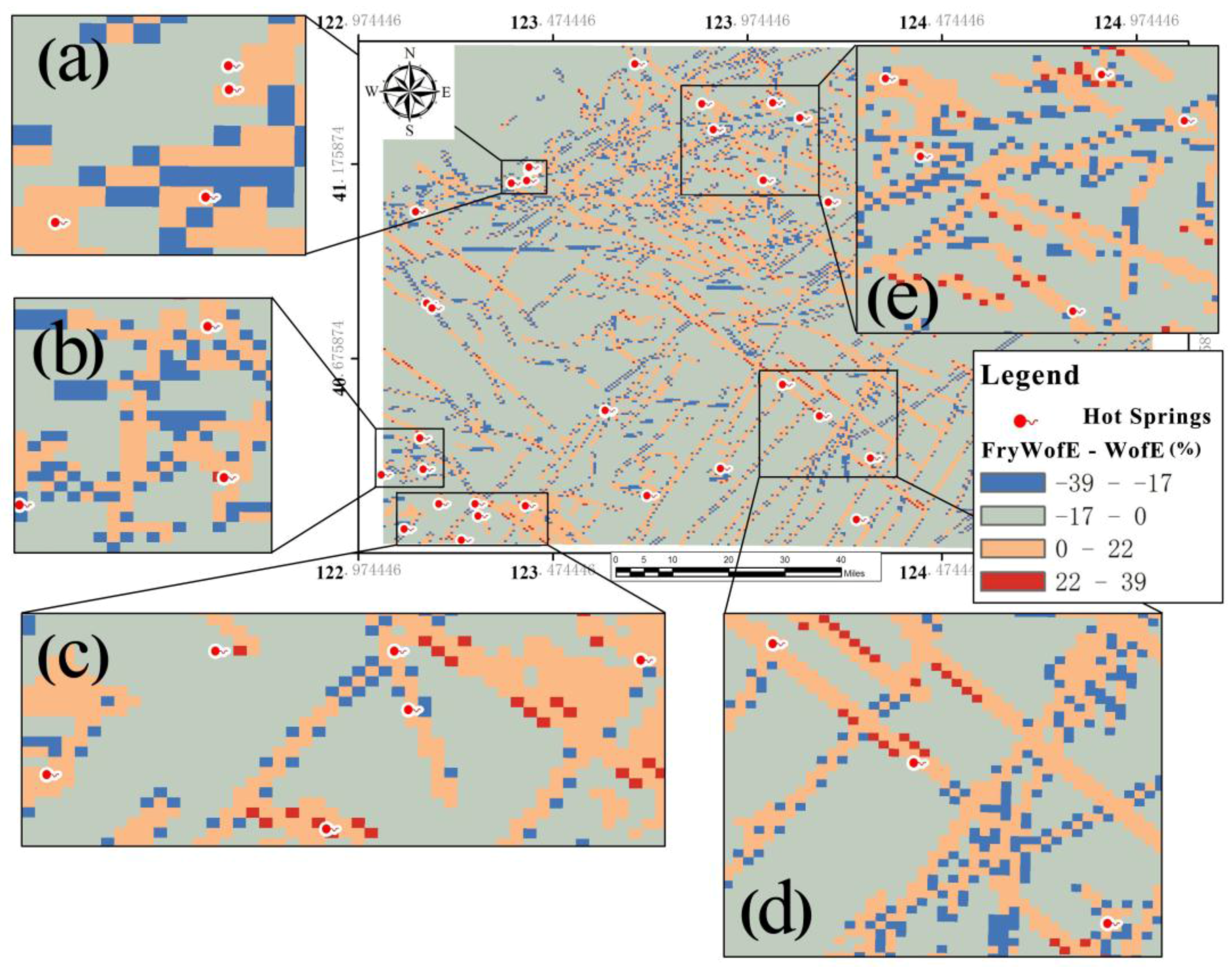
Figure 1.
Geological sketch of the study area, which includes main fault zones; Hanling-Pianling fault zone (HP); Hanling-Benxi fault zone (HB); Haicheng-Caohekou fault zone (HC); Haicheng Ximucheng-Xiuyan fault zone (HX); Daheisha-Zhangjiapu fault zone (DZ); Liujiahe-Qingduizi fault zone (LQ); Sipingjie-Fengcheng fault zone (SF); Zhuanghe-Huanren fault zone (ZH); Erpengdianzi-Changdian fault zone (EC); and the Yalu River fault zone (YL).

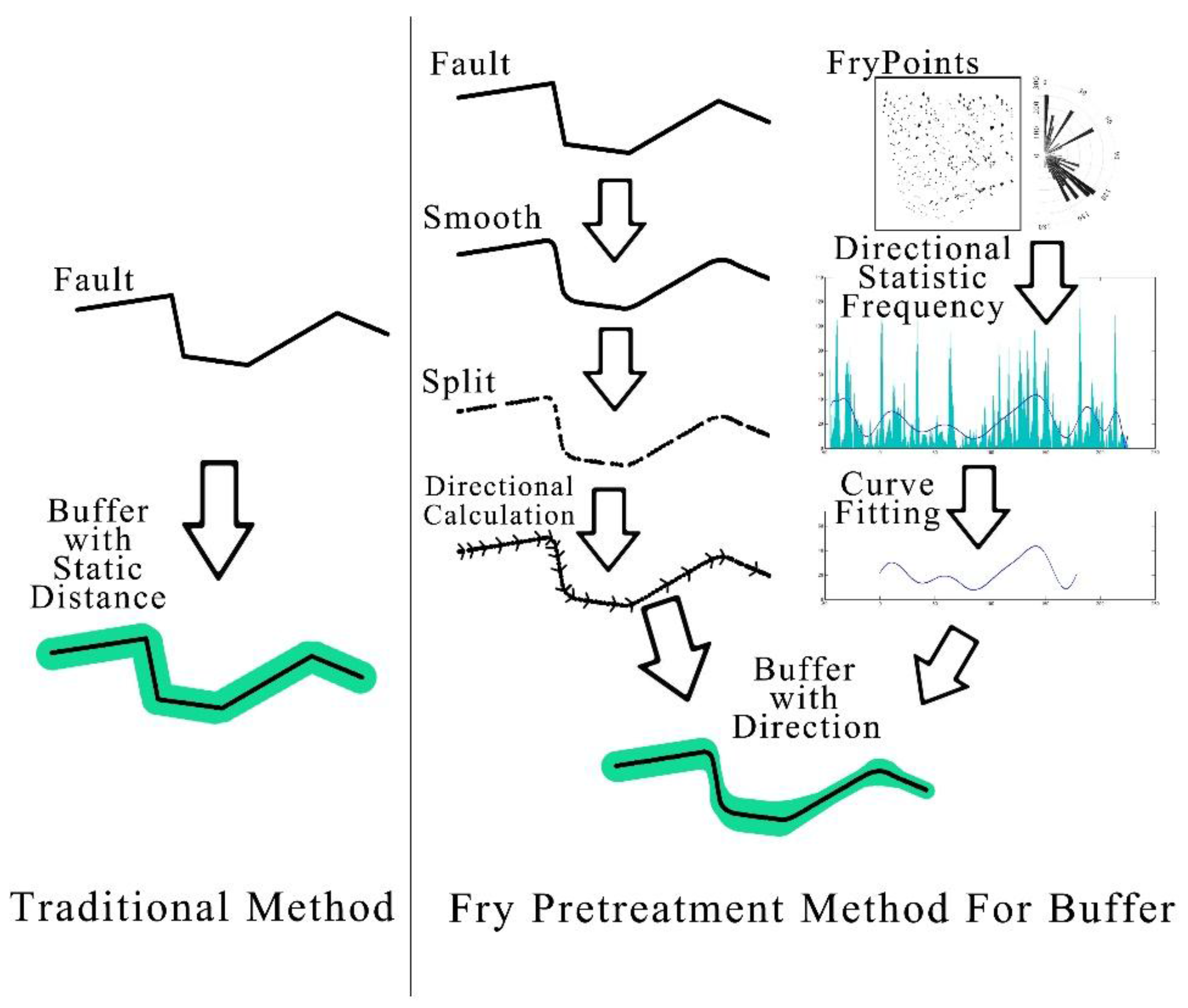
Figure 2.
Workflow for geothermal anomaly analysis based on the Fry-WofE method. The orange rectangle shows the pretreatment processes of the Fry method, including the calculation of the trend direction of the hot spring point distribution and the curve fitting with the use of the Fry analysis result. The weight of the fault is obtained by fitting the curve; the fault buffer area under the influence of weight is calculated with the weight value; and the fault evidence weight layer can be calculated finally.

Figure 3.
Fry method analysis process for hot spring data.

Figure 4.
Results of a Fry analysis of hot springs in eastern Liaoning; the image on the left shows the distribution of Fry points, and the righthand picture represents the angle and quantity of the Fry point distribution.
Figure 4.
Results of a Fry analysis of hot springs in eastern Liaoning; the image on the left shows the distribution of Fry points, and the righthand picture represents the angle and quantity of the Fry point distribution.

Figure 5.
Compared with the original method of (b) fitting (a), the method of (d) fitting (c) can obviously obtain better processing results at both ends of the fitting curve without changing the amount of data. (a) Angle distribution frequency and the 20th fitting curve in the range of 0° to −179°. (b) Fitting curve in the range of 0° to −179°. (c) Angle distribution frequency and the 20th fitting curve in the range −45° to −224° range. (d) Fitting curve of the 20th fitting curve after intercepting the 0° to −179° range.

Figure 6.
The change of the normr value of the fitting curve with the time; the left Y axis and the black node curve indicate the normr value of the curve trend with the number of curves, and the right Y axis and the triangle node curve indicate the trend of the slope of the normr curve with the number of curves.

Figure 7.
Fault buffer flow of the traditional methods and the Fry pretreatment methods.

Figure 8.
Comparison of the area weighted evidence relation curves of a fault buffer treated with the WofE method and the Fry-WofE method. We can see that the “×” node curve has a at peak y = 16 and about x = 4000, and the triangle node curve appears at about y = 13 and x = 6000. The Fry-WofE method is better than the traditional WofE method, regardless of the position or height of the peak. In general, the Fry-WofE method can achieve a higher hit response with a smaller coverage area.

Figure 9.
The relationship between the river network extraction threshold and the total river length in the studied area; the turning point where the river length changes from short to long can be seen in about 800.
Figure 9.
The relationship between the river network extraction threshold and the total river length in the studied area; the turning point where the river length changes from short to long can be seen in about 800.

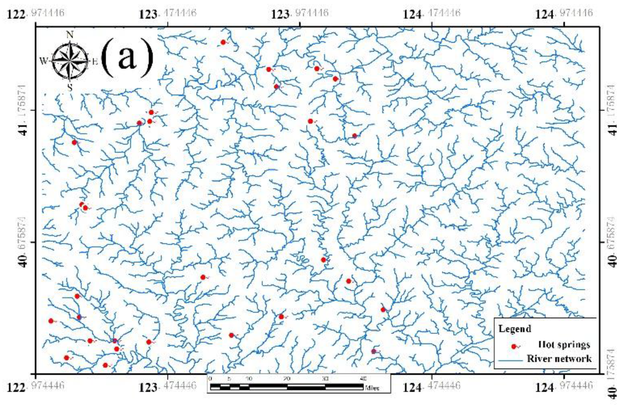
Figure 10.
Evidence of the factor layer, including (a) the distribution map of the river network (b) the map of the distribution of the major lithology (c) standard deviations (STD) of the Bouguer gravity anomaly.
Figure 10.
Evidence of the factor layer, including (a) the distribution map of the river network (b) the map of the distribution of the major lithology (c) standard deviations (STD) of the Bouguer gravity anomaly.


Figure 11.
Comparison of prediction results of geothermal potential between traditional WofE and Fry-WofE methods. (a) The results of geothermal potential evaluation by the traditional WofE method; (b) the results of geothermal potential evaluation by the Fry-WofE method.
Figure 11.
Comparison of prediction results of geothermal potential between traditional WofE and Fry-WofE methods. (a) The results of geothermal potential evaluation by the traditional WofE method; (b) the results of geothermal potential evaluation by the Fry-WofE method.

Figure 12.
Evaluation of the different distributions of the WofE method and the Fry-WofE method with hot springs verified; the red area indicates that the Fry-WofE method suggests that the region is more likely to have hot springs. Figure shows that the Fry-WofE method is better than the traditional WofE method in fitting the existing hot spring points.

Figure 13.
Geothermal prospective area and hot spring prediction points in the Liaodong area with fault and terrain data.
Figure 13.
Geothermal prospective area and hot spring prediction points in the Liaodong area with fault and terrain data.

Table 1.
Fitting curve parameter.
| Param | Value |
|---|---|
| −10.52686667 | |
| −1.027335093 | |
| 164.6139817 | |
| 47.17474773 | |
| −1083.424953 | |
| −488.7698531 | |
| 3908.855178 | |
| 2297.937356 | |
| −8444.631723 | |
| −5802.886174 | |
| 11,229.45373 | |
| 8190.734099 | |
| −9154.66568 | |
| −6239.502558 | |
| 4493.515456 | |
| 2277.87883 | |
| −1322.528323 | |
| −320.2284792 | |
| 230.3176747 | |
| 27.87151178 | |
| 8.563531772 |
Table 2.
Predict hit ratio comparison of the Fry-WofE prediction method and the WofE prediction method.
Table 2.
Predict hit ratio comparison of the Fry-WofE prediction method and the WofE prediction method.
| Prediction Method | Hit Probability of Highly Predictive Potential Region | Hit Probability of Medium Predictive Potential Region | Total Hit Rate |
|---|---|---|---|
| Fry-WofE | 54.5% | 18.2% | 72.7% |
| WofE | 36.4% | 24.2% | 60.6% |
© 2017 by the authors. Licensee MDPI, Basel, Switzerland. This article is an open access article distributed under the terms and conditions of the Creative Commons Attribution (CC BY) license (http://creativecommons.org/licenses/by/4.0/).
Share and Cite
MDPI and ACS Style
Sang, X.; Xue, L.; Liu, J.; Zhan, L. A Novel Workflow for Geothermal Prospectively Mapping Weights-of-Evidence in Liaoning Province, Northeast China. Energies 2017, 10, 1069. https://doi.org/10.3390/en10071069
AMA Style
Sang X, Xue L, Liu J, Zhan L. A Novel Workflow for Geothermal Prospectively Mapping Weights-of-Evidence in Liaoning Province, Northeast China. Energies. 2017; 10(7):1069. https://doi.org/10.3390/en10071069
Chicago/Turabian StyleSang, Xuejia, Linfu Xue, Jiwen Liu, and Liang Zhan. 2017. "A Novel Workflow for Geothermal Prospectively Mapping Weights-of-Evidence in Liaoning Province, Northeast China" Energies 10, no. 7: 1069. https://doi.org/10.3390/en10071069
Note that from the first issue of 2016, this journal uses article numbers instead of page numbers. See further details here.