
A Computational Tool for Comparative Energy Cost Analysis of Multiple-Crop Production Systems
by
 , ,
, ,
Efthymios Rodias
1, 
Remigio Berruto
1,*,
Dionysis Bochtis
2,
Patrizia Busato
1 and
Alessandro Sopegno
1 1
Department of Agriculture, Forestry and Food Science (DISAFA), University of Turin, Largo Braccini 2, 10095 Grugliasco, Italy
2
Institute for Research and Technology—Thessaly IRETETH/Centre for Research & Technology Hellas CERTH, Dimitriados Str. 95, GR 38333 Volos, Greece
*
Author to whom correspondence should be addressed.
Energies 2017, 10(7), 831; https://doi.org/10.3390/en10070831
Submission received: 5 April 2017
/
Revised: 29 May 2017
/
Accepted: 13 June 2017
/
Published: 22 June 2017
(This article belongs to the Collection Bioenergy and Biofuel)
Abstract
:Various crops can be considered as potential bioenergy and biofuel production feedstocks. The selection of the crops to be cultivated for that purpose is based on several factors. For an objective comparison between different crops, a common framework is required to assess their economic or energetic performance. In this paper, a computational tool for the energy cost evaluation of multiple-crop production systems is presented. All the in-field and transport operations are considered, providing a detailed analysis of the energy requirements of the components that contribute to the overall energy consumption. A demonstration scenario is also described. The scenario is based on three selected energy crops, namely Miscanthus, Arundo donax and Switchgrass. The tool can be used as a decision support system for the evaluation of different agronomical practices (such as fertilization and agrochemicals application), machinery systems, and management practices that can be applied in each one of the individual crops within the production system.
1. Introduction
Various crops can be considered as potential bioenergy and biofuel production feedstocks. The selection of the crops to be cultivated for that purpose is based on several factors, including plant requirements, farmers’ preferences, geographical dispersion of the cultivated area, agricultural practices, and available equipment. However, the operational conditions are frequently applicable to the cultivation of more than one crop type. Consequently, an evaluation of the economic or energy benefits between potential crops to be cultivated in an area is required; this also applies in the case of strategic planning in terms of bioenergy crop production within a specific area. The estimation of the energy consumption or energy balance is the outcome of a wide range of parameters. As a result, there is a substantial deviation between different energy input analysis studies. This mainly results from the large number of factors that directly or indirectly affect the energy input. Such factors can be the diversity in agrochemical or fertilizers quantities, the machinery systems used and the geographical deployment of the whole production system. A common framework is thus required in order to compare different crops objectively, taking into account economic or energetic performance criteria.
As already mentioned, a number of different crop production-related factors significantly affect the input requirements of the whole system [1,2]. Different transport distances between the various locations that are involved (e.g., farm, fields and storage facilities), different machinery systems and crop protection used may lead to high variations in the energy input requirements for each individual field. Furthermore, the task durations for the machinery activities are usually based on average norms and do not provide results for the design or evaluation processes of a specific production system [3,4]. To that effect, Sopegno et al. [5] developed a computational tool for the estimation of the energy requirements on individual fields. The tool is based on an in-depth work breakdown accounting of the in-field and transport operations presenting the Miscanthus x giganteus production. The developed tool provides detailed analysis on the energy requirements of the components that contribute to the energy input. However, the tool can only deal with a single crop. In this paper, the computational tool presented in [5] is further extended in order to evaluate the energy cost parameters, such as energy consumption and energy balance, on multiple crops. The proposed tool can thus provide results in a comparison form. The innovation of the presented tool mainly refers to its capability to evaluate any set of crops provided energy-specific and other cultivation-specific inputs either extracted from the literature or real farm data. Furthermore, the tool can be dynamically expanded through the update of the embedded databases, as well as through the inclusion of various agricultural production practices for the individual case scenarios.
The structure of the present work is as follows: initially, a brief presentation of the tool in terms of the main input parameters and functionalities is provided. Then a demonstration scenario is described which is based on three selected energy crops, namely Miscanthus, Arundo donax and Switchgrass. This is followed by the results section, where a comparison between the various energy costs for the three crops is presented. The paper wraps up with the conclusions of the work.
2. The Computational Tool
It should be highlighted that the presented tool is an extension of an existing one presented in Sopegno et al. [5]. The latter was initially developed for the analysis of the Miscanthus production and transportation processes. In this work, the tool developed by Sopegno et al. is modified and further extended in order to deal with multiple-crops that are produced in the same production system. The system boundary remains similar since it includes the in-field operations, the transportations of the machinery from farm to field, the transportation of the material e.g., fertilization) to the field and the transportation of the produced biomass from the field to the biomass storage or processing facilities (Figure 1).
The input parameters that are included can be classified in four main categories:
- General production inputs, which include the field (e.g., field area) and the crop parameters (e.g., crop yield).
- Field and transport operations inputs, which include all the parameters related to operations (in-field and transport) that are performed each year for each crop, as well as any other related parameter (e.g., operating speed).
- Field machinery inputs, which include the tractor-specific parameters (e.g., tractor power, tractor weight, machinery embodied energy) and the equipment-specific parameters (e.g., operating width).
- Material specific inputs, which include the embodied energy and the material used, such as agrochemicals, fertilizers and propagation means.
The term “embodied energy” refers to the summation of the used energy during production of the raw materials, the required energy during manufacture, the transport energy required to reach the consumer and the consumed energy in maintenance works, both for agrochemical/fertilization material and machinery input [6].
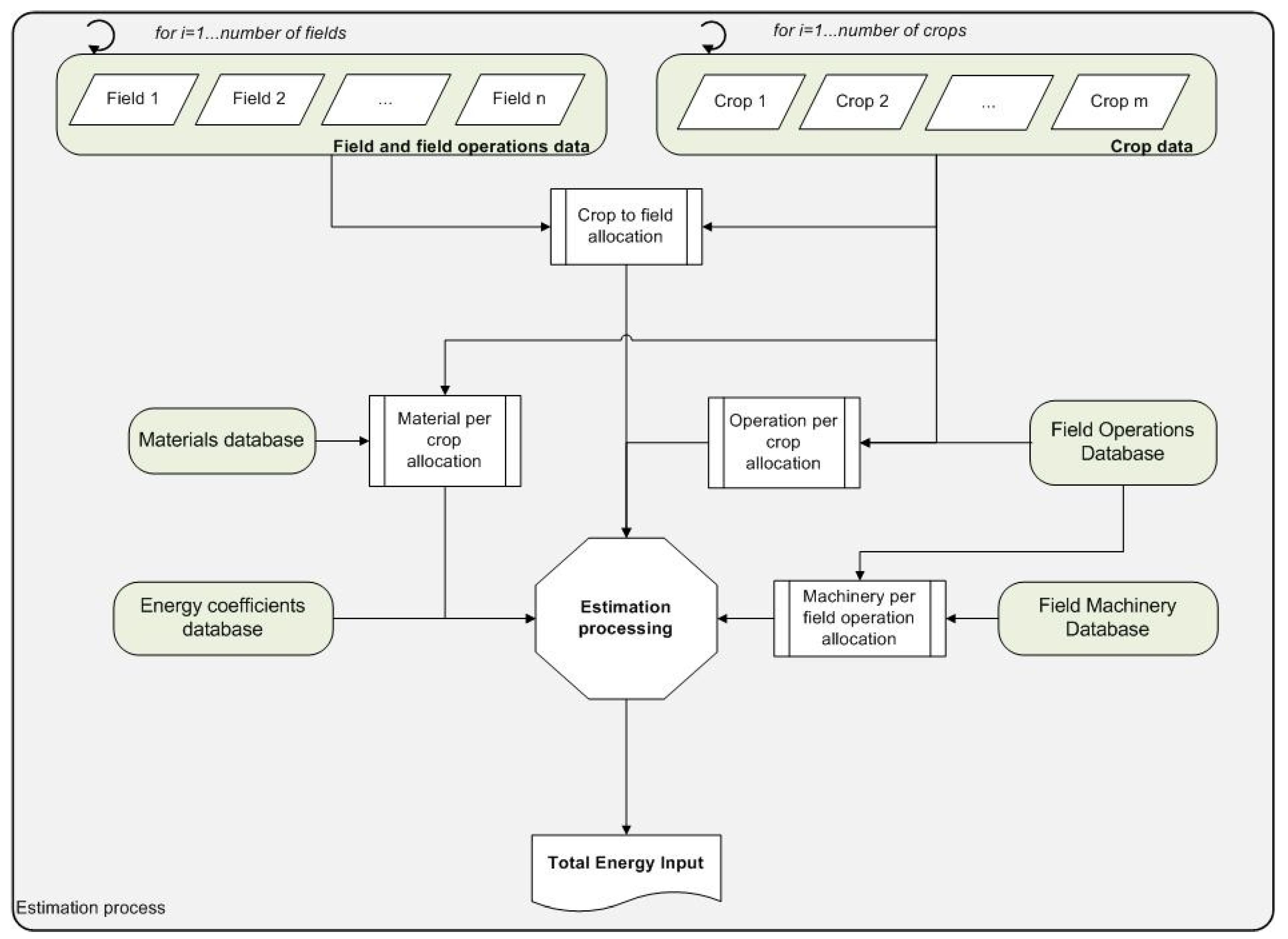
Figure 2 illustrates the general process of the energy input estimation. Each field and crop data are selected in combination with the corresponding field machinery that are used for each specific case and the material data, the process occurs.
The field operations can be classified into two main categories: (a) the operations that do not include any material flow inputs and; (b) the operations that include material flow inputs. In both categories, the energy consumption is estimated given the in-field operations energy consumption and the farm-to-field transport energy consumption. The difference between the two cases lays in the fact that when there is material flow input, the material embodied energy should be added. Moreover, the material-connected transportation may vary according to the number of trips that should be carried out for the specific material quantity. As regards the energy consumption which results from the transportation of the biomass, the cycle time should be calculated by using traveling times and also unloading time. This cycle time is required so as to calculate the number of transport tractor-wagon sets required to support the entire procedure. The cycle time is directly connected to the harvesting operation in order to avoid interruption in harvesting due to missing of co-travelling tractor-wagon set.
3. Case Study Description
3.1. The Selected Crops
The case study for the demonstration of the tool refers to a production system that includes three energy crops. More specifically, in the present work the production system includes Miscanthus, Arundo donax, and Switchgrass. In the material to follow, the agronomical features of the aforementioned crops are presented.
Miscanthus is a perennial grass-crop, which is characterized by a high lignocellulosic fiber content. It belongs to the C4 photosynthetic pathway plants. Among the various species (fifteen in total), Miscanthus x giganteus normally exceeds 10 years of lifetime. It can reach a plant height of up to 7 m, producing very high dry matter yields under optimal conditions. In addition, Miscanthus is characterized by its facile adaptation to a wide range of different climatic conditions and soil environments [7]. Given the above, Miscanthus is considered a crop with a high potential for energy production [8]. Several studies have been conducted with a focus on accounting the energy requirements of Miscanthus production. More specifically, Angelini et al. [9] estimated for a twelve-year cycle production of Miscanthus that the energy input for the first year accounts to 17 GJ·ha−1 and for each other year to 12.1 GJ·ha−1. Sopegno et al. [5] reported an energy input of 14.8 GJ·ha−1·year−1 for a ten-year Miscanthus production cycle. With regard to a five-year cycle, Mantineo et al. [10] resulted to an energy consumption of 34 GJ·ha−1 in the first year, 22 GJ·ha−1 for the 2nd and 3rd year and only 2.8 GJ·ha−1 for the last two years.
Arundo donax (also known as giant reed) is a perennial crop with a number of features enhancing its potential as an energy crop. It also grows in a wide range of climatic conditions [11]. Furthermore, certain wild, unimproved populations can give yields of up to 40 t·ha−1 of dry matter [7,9]. Giant reed can grow on almost any soil type and it has a robust root system that can make it a quite aggressive plant [8,9]. Angelini et al. [9] reported an energy consumption of 17 GJ·ha−1 for the first year and 12.1 GJ·ha−1 for each following year in a 12-year production period. In another energy analysis of the giant reed, the estimated energy input varied from approximately 39 to 179 GJ·ha−1 for unfertilized and fertilized crops, respectively, in a ten-year cycle production [12]. Finally, an energy cost of 34 GJ·ha−1 in the first year, 22 GJ·ha−1 for the second and third year and only 2.8 GJ·ha−1 for the fourth and fifth year has presented in a five-year cycle production [10].
Switchgrass is a warm season, perennial grass. It grows up to 50–250 cm in height, depending on the specific variety and climatic conditions. Its yield may vary from 6 t·ha−1 of dry matter, at low fertility sites, up to 25 t·ha−1 of dry matter, at highly fertile sites [13]. Switchgrass has many positive characteristics as a potential biomass crop. The most important ones are the high net energy production and the large range of geographical and soil types adaptation [9,11,12,14]. According to Schmer et al. [15], Switchgrass input energy requirements consumption can reach up to 2 GJ·ha−1 for the establishment year and about 5 GJ·ha−1 for each following years. Farrell et al. [16] reported an energy requirement of 7.5 GJ·ha−1 and the energy requirement given by Wang [17] is about 12 GJ·ha−1. Similar results regarding switchgrass have been stated by Sokhansanj et al. [18], with an energy cost of 7.2 GJ·ha−1.
3.2. Production Scenario
The production case studies of the three crops are based on the prevailing production practices followed by farmers and already described in the literature. The production-related parameters (field operations series, implemented machinery, applied dosages of agrochemicals and fertilizers, plant density, etc.) were selected in all cases after a peer review of the related bibliography and according to the real commercial data in order to be as close to the real production procedure as possible. In this study, the three crops are demonstrated in a ten-year production period. The operations that take place each year for each crop are listed in Table 1. It should be highlighted that a micro-irrigation system with all the correlated input parameters is considered for each one of the three individual crops.
3.2.1. Miscanthus Production
Considering the Miscanthus case study, cultivation of the plant does not require any special soil management [9]. For this reason, a light plowing to 20 cm depth and a disk-harrowing operation were considered as the basic soil preparation steps. Directly after the soil preparation and before the crop establishment, it is important to carry out weed control thoroughly in order to minimize the competitiveness of weeds towards the new Miscanthus plants. After the first growth, there is no need for weed control since the crop can protect itself from the weeds. In the present work, a single herbicide application has been considered as pre-planting weed control in the first year.
Since Miscanthus is planted by rhizomes, a row crop planter similar to the potato seed planter was adopted for the planting operation. In general, the plant population should be approximately between 10,000 and 12,000 plants per ha [19]. Given the fact that there will be establishment losses of 30–40% on average [15,20], approximately 15,000 to 17,000 rhizomes per ha are required to reach the final recommended healthy plant density. In this case study, 16,000 rhizomes per ha have been considered.
The irrigation of the new plants during the first growing season improves establishment success [21]. Irrigation is applied every year in parallel with rainfall in order to cover water requirements and ensure considerable yields. In case under study, 450 mm of irrigation needs has been included [10].
Normally, Miscanthus has low nutrient requirements since the crop itself can absorb most of the required nutrients from the soil. However, the addition of nitrogen, phosphorus and potassium might be necessary, depending on the specific nutrient soil conditions. It has been reported that fertilizer quantities of 50 kg N, 21 kg P2O5, and 45 kg K2O per ha and year are sufficient to support adequate yields [14]. This nutrient allocation has been also implemented in the presented study.
Harvesting of the crop usually occurs every year, starting from the second year onwards. At the end of the growing season, Miscanthus usually drops most of its leaves as it senesces, and the senesced stems are typically harvested from November until late March [22]. Harvesting is usually carried out using conventional forage harvesters for cutting and chopping the biomass. This is supported by transportation vehicles (usually a combination of tractor-wagon) moving in parallel to the harvester for unloading the processed material. The yield of the crop was taken equal to 21.87 t·ha−1 corresponding to the energy content of the harvested biomass equal to 16.4 MJ·kg−1 of dry matter [10].
3.2.2. Arundo donax Production
Cultivation of Arundo donax has no special soil preparation requirements [14]. In this light, in the Arundo donax case study, a plowing to 20 cm depth and a disk-harrowing were considered as sufficient. Subsequently and before planting, a weed control operation was considered. No weed control was considered for the following years due to the crop’s physical potential to compete with weeds by itself.
Arundo donax is a seedless plant; it is usually propagated by rhizomes [11]. The plant population may vary from 20,000 to 40,000 plants per ha, even though it has been reported that 20,000 plants per ha give higher energy efficiency [12]. In the present case study, a plant population of 20,000 plants per ha was considered. Similar to the Miscanthus case as described above, irrigation was applied each year in order to cover the water requirements in parallel with rainfall. Thus, 450 mm of irrigation water was considered [10].
Regarding fertilization, annual applications of nitrogen are recommended at a level up to 100 kg·ha−1, especially in nitrogen-poor soils. Moreover, it is essential before the establishment to incorporate sufficient phosphorus into the soil by plowing in a quantity of 200 kg·ha−1 as a minimum, especially in phosphorus-poor fields. Potassium fertilization should be applied only where it is required [8,9]. In the present case study, for the first year the application of 80 kg·ha−1 N, 200 kg P2O5 and 100 kg·ha−1 K2O was considered. For each even year (2nd, 4th, 6th, 8th and 10th year) 80 kg·ha−1 N and 50·ha−1 kg P2O5, was considered. For each odd year, except of the first one (3rd, 5th, 7th and 9th), the application of 80 kg·ha−1 N, 50 kg·ha−1 P2O5 and 100 kg·ha−1 K2O was considered.
Arundo donax can be harvested usually every year or every second year in autumn or in winter [12]. At the presented case, harvesting was considered for every year, starting from the second year onwards. Similar to the Miscanthus case, the harvesting process is carried out by forage harvesters in combination with tractor-wagons for the collection of the harvested material. The yield of the crop was considered 32.95 t·ha−1 corresponding to the energy content of 16.4 MJ·kg−1 of dry matter [10].
3.2.3. Switchgrass Production
In Switchgrass cultivation, seedbeds are normally prepared by traditional plowing and secondary cultivation processes in order to produce a firm seedbed with a fine-textured surface. In the present case study, plowing and disk harrowing were considered for the soil preparation. During the first growth, it is important for the seedbed to have been weed controlled thoroughly because Switchgrass is not competitive during the first establishment phase [23]. Before seeding, a pre-seeding herbicide control was considered in the presented study.
Switchgrass is established by seed. The number of plants established can be up to 400 plants per m2, depending upon weed control strategy after sowing [6,14]. However, towards establishing a healthy plant, a planting density of 10–20 per m2 is considered to be adequate [18,23]. In the present case study, a plant density of 150,000 plants per ha was determined.
As in the previously described crops, apart from rainfall, irrigation is important in order to achieve significant yields. For this reason, water application of 240 mm is adopted in order to cover the annual water needs of Switchgrass [13].
Regarding fertilization, Switchgrass can produce high yields even under limited fertilization of 75 kg N·ha−1 [8]. In the first year, no nitrogen should be applied, as it can promote weed growth leading to competition against the new plants. Phosphorus and potassium should be applied if soil availability is low. In the following years, production application of nutrients should be at a level that anticipates rising productivity taking also into account losses of minerals in the harvested biomass [9]. In the presented case study, the following fertilization plan was considered. During the first year 100 kg·ha−1 P2O5 and 100 kg·ha−1 K2O are applied. During the second year no fertilization was realized. In the following odd years (3rd, 5th, 7th and 9th) 75 kg N·ha−1, 100 kg·ha−1 P2O5 and 100 kg·ha−1 K2O was applied, while in the following even years (4th, 6th, 8th and 10th) the application of only 75 kg N·ha−1 was considered.
As regards herbicides, Switchgrass growth is slow in the first year and there is a negative competition with weeds. It is important for the crop to survive the first winter and re-grow in spring [9]. Thus, Switchgrass requires weed control, not only before establishment, but also for the next two years. In the case study herein presented, atrazine application of 1.12 kg·ha−1 was considered for application before the establishment and 2,4-D application of 4.26 kg·ha−1 for application in the second and third year [19,24].
For harvesting operation, there is no technical reason so as the crop not be cut and harvested by traditional grass harvesting machinery [23]. Switchgrass does not perform well when harvested frequently. Thus, 1–2 cuts per year are usually realized [8]. In the presented case, one cut per year was considered, starting from the second year. Before the forage harvester operates, a mowing operation is considered in order to allow adequate time to the mowed plants to get dry during winter [23]. The most frequently observed Switchgrass yield among different soils and management practices varies between 10 and 12 t·ha−1 [25]. In the present case study, a yield of 11 t·ha−1 with energy content of 19.2 MJ·kg−1 of dry matter was considered [18].
3.3. Input Parameters
The energy inputs regarding the propagation means for Miscanthus and Arundo donax production are based on the work of Mantineo et al. [10] that gives 0.00552 MJ per rhizome. For Switchgrass production, the energy input from Switchgrass seeds was adopted equal to 0.002 MJ·m−2, given the fact that an average plant density in Switchgrass production systems demands seeds in the density of 0.0007 kg·m−2 [19,23].
The field machinery related inputs that included in all of the presented cases are detailed in Table 2. The energy inputs regarding the transportation operations and the irrigation connected energy factors are listed in Table 3 and Table 4, respectively.
In the production scenario chapter, the analysis of the annual applications of fertilizers and agrochemicals has already presented for each of the crops. The corresponding energy factors that are included in fertilization are 78.1 MJ·kg−1 for nitrogen, 17.4 MJ·kg−1 for phosphorus and 13.7 MJ·kg−1 for potassium [6]. Regarding agrochemicals application, only herbicide application was implemented in Miscanthus and Switchgrass. The energy factors were 454 MJ·kg−1 of ai for Glyphosate [6], 190 MJ·kg−1 of ai for Atrazine [26] and 85 MJ·kg−1 of ai for 2,4-D [27]. Glyphosate was considered for Miscanthus and the other two herbicides were implemented in Switchgrass crop. Regarding Switchgrass there is no need for any herbicide application if rhizomes are used for the establishment of the crop [14].
4. Results
4.1. Basic Scenarios
For each one of the three examined crops in the present study, a unit area of one-hectare field was considered. The area is located 5 km from the farm and 10 km from the biomass storage facilities. The field areas implemented for the simulation runs are located in Crescentino, in the Piedmont region near the Chemtex biofuel plant, in the Northern part of Italy. Given all the energy inputs and other parameters, the energy consumption per operation was calculated for each one of the energy crops. The energy consumption per field operation is depicted in Table 5.
The total energy consumption of the presented crops can be up to 20.3 GJ·ha−1·year−1 for Miscanthus, 20.9 GJ·ha−1·year−1 for Arundo donax and 14.1 GJ·ha−1·year−1 for Switchgrass. This annual energy consumption is the average annual of the total energy consumption for a 10-year period. That reflects the fact that the energy input may differ from year to year due to different field operations that are considered or due to variable material inputs that are taken into account on each occasion.
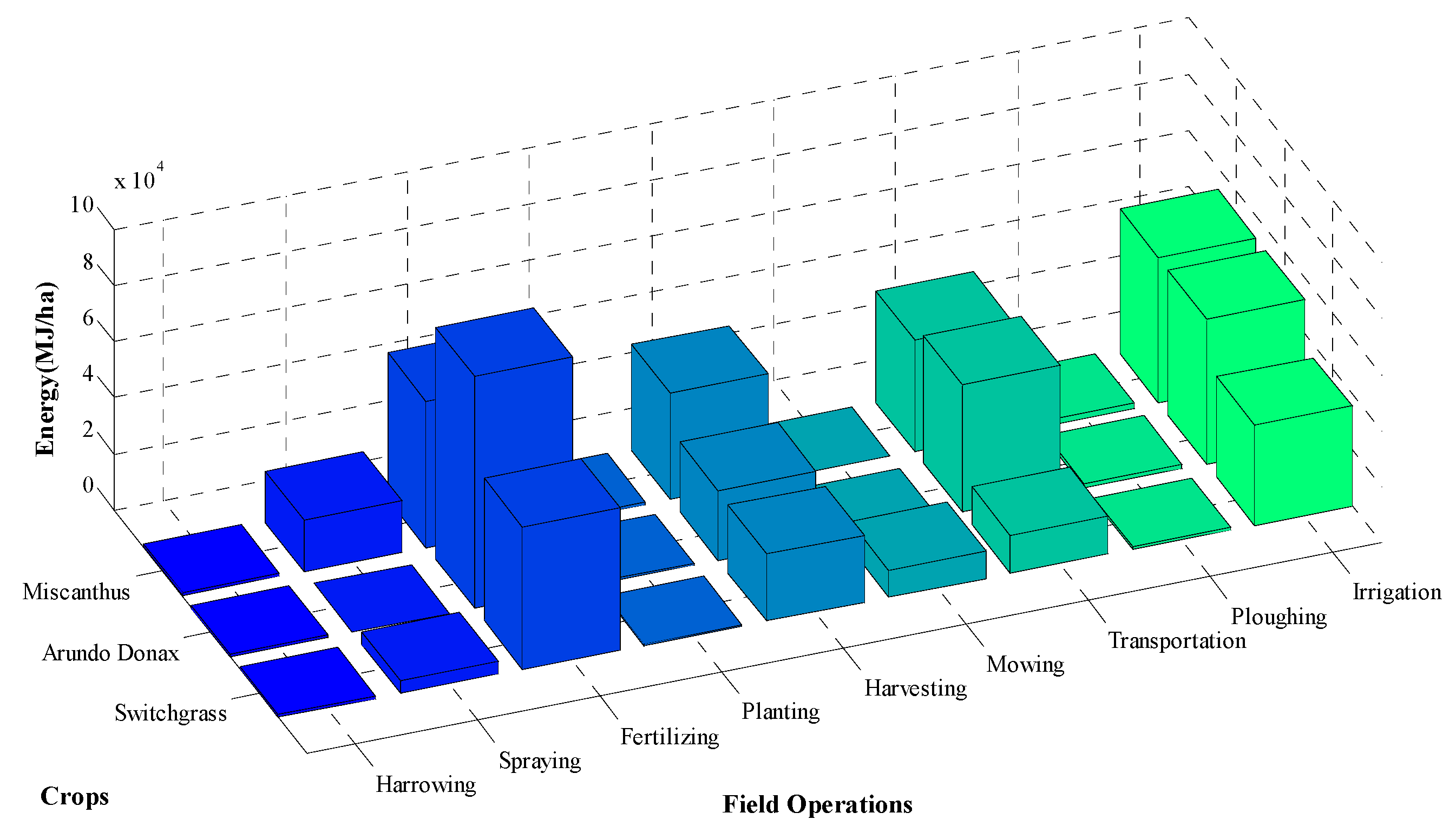
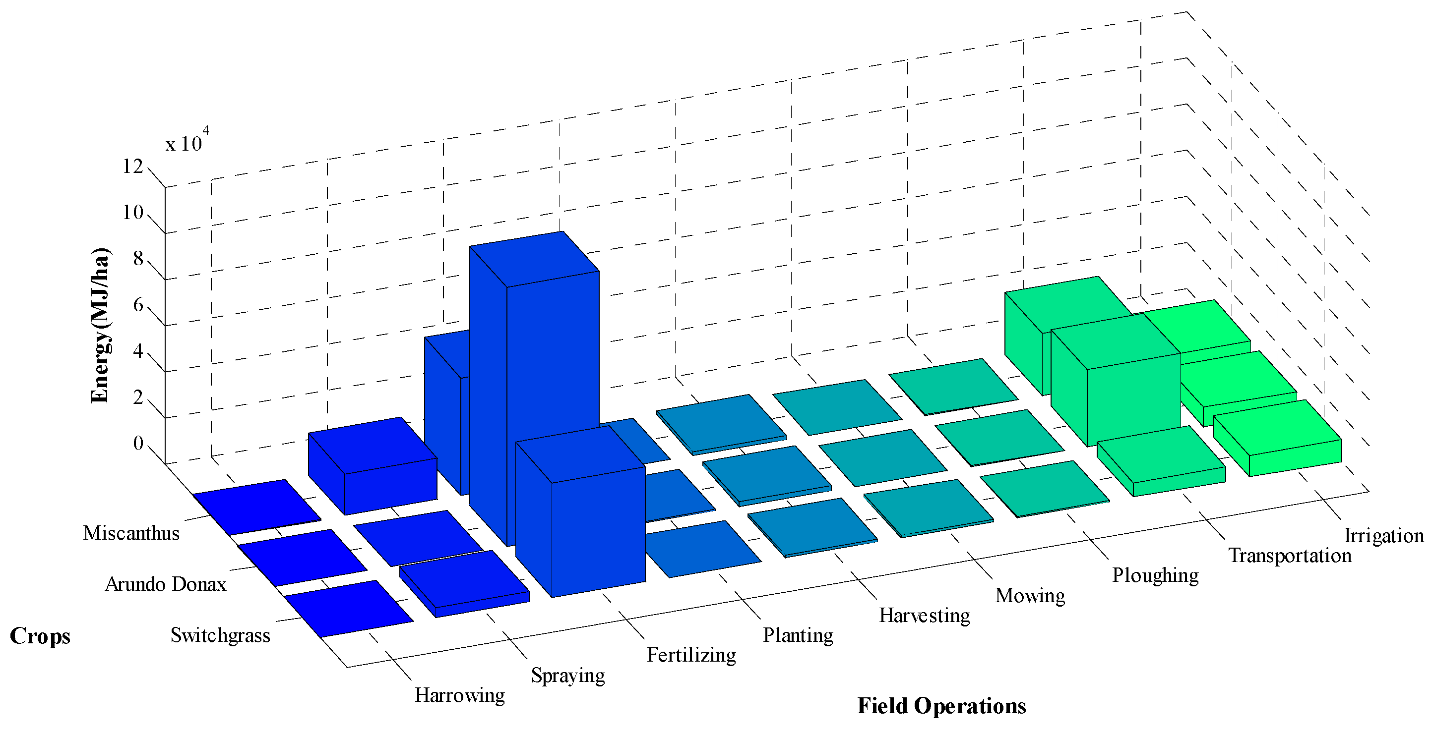
Figure 3 graphically illustrates the energy contribution per crop. The figures sum up all the field operations that take place during the 10-year period. The energy consumption that corresponds to fuels consumption for each field operation and each crop is shown in Figure 4. Figure 5 presents the energy contribution that comes from embodied energy for each field operation and crop.
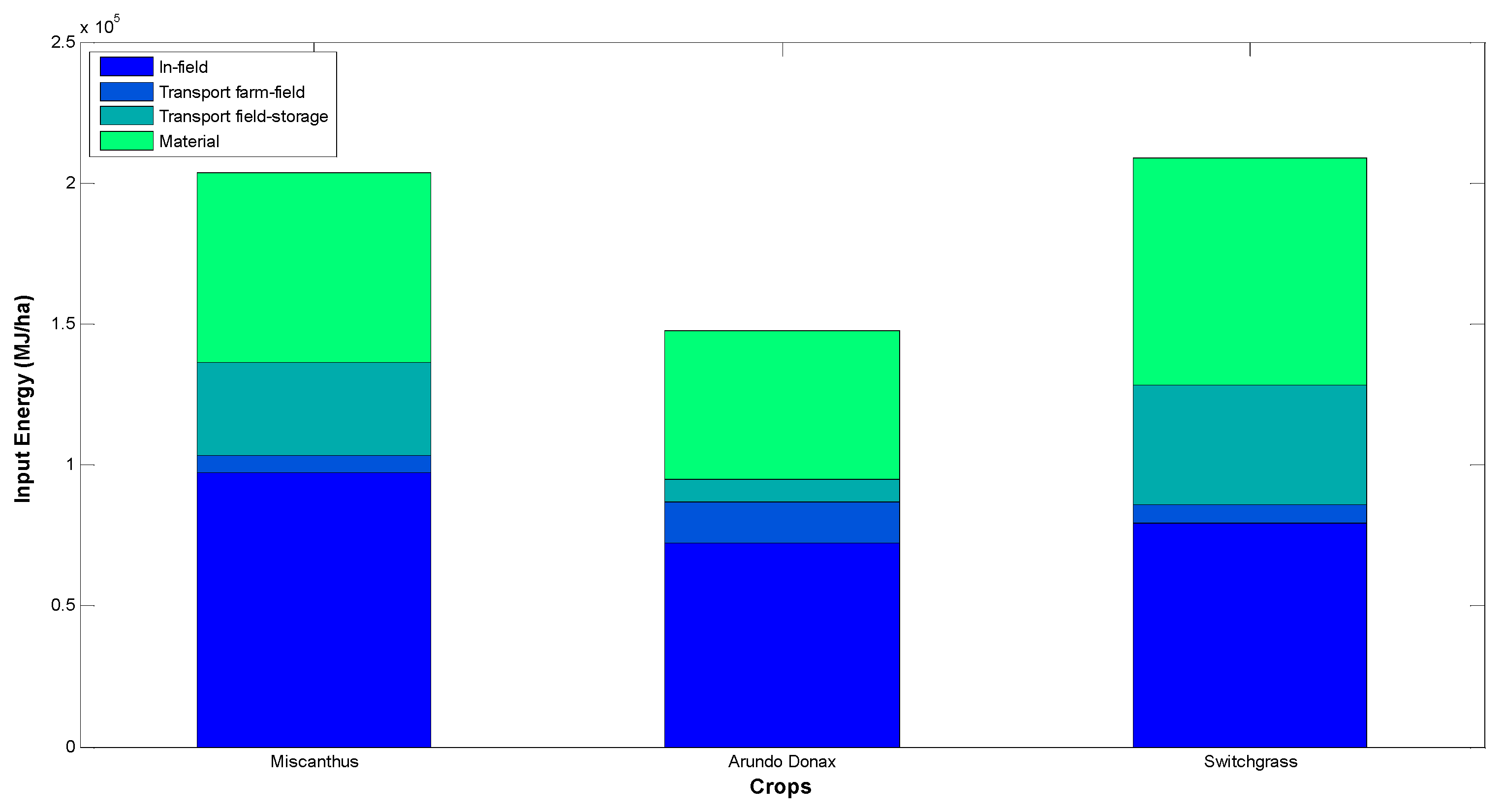
The main energy factors were allocated in three main categories. More specifically, the in-field operations, the farm-field transport operations and the field to storage transport of the harvested product are considered. In addition to these three main energy factors, the material (agrochemicals, etc.) energy contribution has been included. The input energy distribution in MJ·ha−1 for the three crops for ten years cycle is graphically depicted in Figure 6.
The total energy cost of each crop is connected directly to other energy expressions as already described by Sopegno et al. [5]. In the present case study, the total energy input (EI) and the total energy output (EO), both expressed in GJ (in our case, the scenarios referred to fields of 1 ha) and GJ·ha−1, the efficiency of energy (EoE) (extracted from EOU/EIU) and energy balance (EB) in GJ·ha−1 (extracted from EOU-EIU) are also calculated and presented in Table 6 for the three crops.
4.2. The Effect of Distance
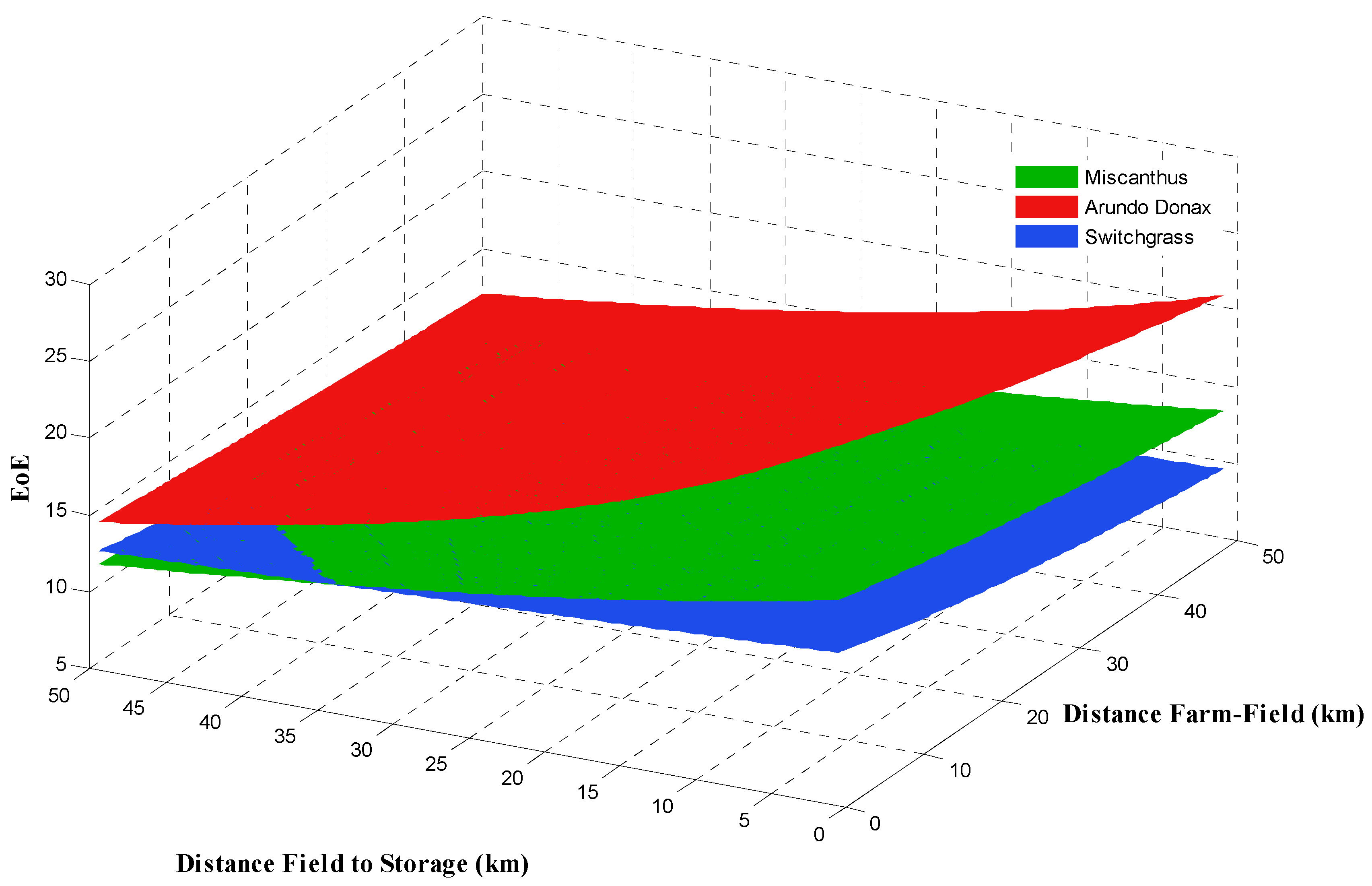
The transportation system has a significant effect in the energy requirements of any given crop, considering the required number of trips in each field operation. Apart from the number of trips, transportation energy requirements are directly connected to the number of vehicles that are necessary for an operation, the utilization level of a unit and the idle times (loading/unloading times, time to connect or disconnect field machinery implements etc.). As already mentioned, in the present work, transportation is divided as follows: (a) from farm to field, which may include material (fertilizers etc.) transportation apart from the machinery transport and; (b) transportation from field to storage facilities, which is directly connected only to harvesting. In Figure 7, the variable effect of these two distances on the EoE is illustrated as surfaces for the three crops, regarding distances, farm-to-field and field-to-storage, that vary from 1 to 50 km. As shown in Figure 7, there is an interception between Miscanthus and Switchgrass. The interception occurs when both the field-to-storage distance is higher than 35 km and the farm-to-field distance is less than 10 km. At this case, Switchgrass is shown to have higher EoE compared to the Miscanthus.
5. Conclusions
A computational tool for the simultaneous energy and cost evaluation for multiple-crop production systems is presented. All the in-field and transport operations are taken into account, thus providing a detailed analysis of the energy requirements of the components that contribute to the total energy consumption. The tool can be used in the design or the evaluation of specific biomass productions systems. Furthermore, it can be used as a decision support tool for the evaluation of different agronomical practices that can apply in each one of the tested crops (such as different quantities or types in irrigation, fertilization and agrochemicals application). The individual field-specific outputs of this tool make it feasible for its implementation in crop allocation problems, as an optimization process in fields that are geographically dispersed, for example, around a bioenergy plant in order to maximize the net energy production. Furthermore, given the fact that the final product delivered to a bioenergy plant should follow very specific prerequisite and, also, given the competitiveness of the market regarding the green production that should be followed, the comparison of energy cost analysis regarding energy crops is significant in order to acquire the maximum possible biomass by using the optimal energy crops that minimize the total energy cost.
The tool could be used to predict some performance indicators for many scenarios. This will help to design web apps to browse a database where the scenarios, already calculated with this tool are stored and retrieved for the final user.
Acknowledgments
The authors thank the University of Turin for the financial support to carry out the research.
Author Contributions
Efthymios Rodias implemented the Matlab code and wrote the paper; Dionysis Bochtis designed the tool and wrote the paper; Patrizia Busato analysed the data; Remigio Berruto validated the results; Alessandro Sopegno elaborated the results.
Conflicts of Interest
The authors declare no conflict of interest.
Abbreviations
The following abbreviations are used in this manuscript:
| EI | Energy Input |
| EO | Energy Output |
| EIU | Energy Input per unit area |
| EOU | Energy Output per unit area |
| EoE | Efficiency of energy |
| EB | Energy balance |
References
- Ren, L.; Cafferty, K.; Roni, M.; Jacobson, J.; Xie, G.; Ovard, L.; Wright, C. Analyzing and comparing biomass feedstock supply systems in China: Corn stover and sweet sorghum case studies. Energies 2015, 8, 5577–5597. [Google Scholar] [CrossRef]
- Busato, P.; Berruto, R. A web-based tool for biomass production systems. Biosyst. Eng. 2014, 120, 102–116. [Google Scholar] [CrossRef]
- Castillo-Villar, K.K.; Minor-Popocatl, H.; Webb, E. Quantifying the impact of feedstock quality on the design of bioenergy supply chain networks. Energies 2016, 9, 203. [Google Scholar] [CrossRef]
- Puigjaner, L.; Pérez-Fortes, M.; Laínez-Aguirre, J.M. Towards a carbon-neutral energy sector: Opportunities and challenges of coordinated bioenergy supply Chains-A PSE approach. Energies 2015, 8, 5613–5660. [Google Scholar] [CrossRef]
- Sopegno, A.; Rodias, E.; Bochtis, D.; Busato, P.; Berruto, R.; Boero, V.; Sørensen, C. Model for energy analysis of Miscanthus production and transportation. Energies 2016, 9, 392. [Google Scholar] [CrossRef]
- Kitani, O. CIGR Handbook of Agricultural Engineering Volume V; CIGR–The I.; ASAE Publication: St. Joseph, MI, USA, 1999; Volume V. [Google Scholar]
- Vermerris, W. Genetic Improvement of Bioenergy Crops; Springer: Berlin, Germany, 2008. [Google Scholar]
- Atkinson, C.J. Establishing perennial grass energy crops in the UK: A review of current propagation options for Miscanthus. Biomass Bioenergy 2009, 33, 752–759. [Google Scholar] [CrossRef]
- Angelini, L.G.; Ceccarini, L.; Nassi o Di Nasso, N.; Bonari, E. Comparison of Arundo donax L. and Miscanthus x giganteus in a long-term field experiment in Central Italy: Analysis of productive characteristics and energy balance. Biomass Bioenergy 2009, 33, 635–643. [Google Scholar] [CrossRef]
- Mantineo, M.; D’Agosta, G.M.; Copani, V.; Patanè, C.; Cosentino, S.L. Biomass yield and energy balance of three perennial crops for energy use in the semi-arid Mediterranean environment. Field Crops Res. 2009, 114, 204–213. [Google Scholar] [CrossRef]
- Lewandowski, I.; Scurlock, J.M.O.; Lindvall, E.; Christou, M. The development and current status of perennial rhizomatous grasses as energy crops in the US and Europe. Biomass Bioenergy 2003, 25, 335–361. [Google Scholar] [CrossRef]
- Angelini, L.G.; Ceccarini, L.; Bonari, E. Biomass yield and energy balance of giant reed (Arundo donax L.) cropped in central Italy as related to different management practices. Eur. J. Agron. 2005, 22, 375–389. [Google Scholar] [CrossRef]
- Christian, D.G.; Elbersen, H.W.; Bassam, N.E.; Sauerbeck, G.; Alexopoulou, E.; Sharma, N.; Piscioneri, I.; de Visser, P.; van den Berg, D. Switchgrass (Panicum virgatum L.) as an Alternative Energy Crop in Europe—Initiation of a Productivity Network; Agrotechnological Research Institute: Wageningen, The Netherlands, 2001. [Google Scholar]
- Bassam, N.E. Handbook of Bioenergy Crops: A Complete Reference to Species, Development and Applications; Earthscan: London, UK, 2010. [Google Scholar]
- Schmer, M.R.; Vogel, K.P.; Mitchell, R.B.; Perrin, R.K. Net energy of cellulosic ethanol from switchgrass. Proc. Natl. Acad. Sci. USA 2008, 105, 464–469. [Google Scholar] [CrossRef] [PubMed]
- Farrell, A.E.; Plevin, R.J.; Turner, B.T.; Jones, A.D.; O’Hare, M.; Kammen, D.M. Ethanol can contribute to energy and environmental goals. Science 2006, 311, 506–508. [Google Scholar] [CrossRef] [PubMed]
- Wang, M.Q. Development and Use of GREET 1.6 Fuel-Cycle Model for Transportation Fuels and Vehicle Technologies; Anl/Esd/Tm-163; Argonne National Laboratory: Lemont, IL, USA, 2001.
- Sokhansanj, S.; Mani, S.; Turhollow, S.; Kumar, A.; Bransby, D.; Lynd, L.; Laser, M. Large-scale production, harvest and logistics of switchgrass (Panicum virgatum L.)—Current technology and envisioning a mature technology. Biofuels Bioprod. Biorefin. 2009, 3, 124–141. [Google Scholar] [CrossRef]
- Pyter, R.; Heaton, E.; Dohleman, F.; Voigt, T.; Long, S. Agronomic experiences with Miscanthus x giganteus in Illinois, USA. Methods Mol. Biol. 2009, 581, 41–52. [Google Scholar] [PubMed]
- Garten, C.T.; Smith, J.L.; Tyler, D.D.; Amonette, J.E.; Bailey, V.L.; Brice, D.J.; Castro, H.F.; Graham, R.L.; Gunderson, C.A.; Izaurralde, R.C.; et al. Intra-annual changes in biomass, carbon, and nitrogen dynamics at 4-year old switchgrass field trials in west Tennessee, USA. Agric. Ecosyst. Environ. 2010, 136, 177–184. [Google Scholar] [CrossRef]
- Lewandowski, I.; Clifton-Brown, J.C.; Scurlock, J.M.O.; Huisman, W. Miscanthus: European experience with a novel energy crop. Biomass Bioenergy 2000, 19, 209–227. [Google Scholar] [CrossRef]
- Heaton, E.A.; Dohleman, F.G.; Miguez, A.F.; Juvik, J.A.; Lozovaya, V.; Widholm, J.; Zabotina, O.A.; McIsaac, G.F.; David, M.B.; Voigt, T.B.; et al. Miscanthus. A Promising Biomass Crop. Adv. Bot. Res. 2010, 56, 76–137. [Google Scholar]
- Piscioneri, I.; Pignatelli, V.; Palazzo, S.; Sharma, N. Switchgrass production and establishment in the Southern Italy climatic conditions. Energy Convers. Manag. 2001, 42, 2071–2082. [Google Scholar] [CrossRef]
- Caslin, B.; Finnan, J.; Easson, L. Miscanthus Best Practice Guidelines; Teagasc and Agri-Food and Biosciences Institute: Belfast, UK, 2011.
- Hood, E.E.; Nelson, P.; Powell, R. Plant Biomass Conversion; Wiley-Blackwell: Hoboken, NJ, USA, 2011. [Google Scholar]
- Renz, M.; Undersander, D.; Casler, M. Establishing and Managing Switchgrass. Available online: http://fyi.uwex.edu/forage/establishing-and-managing-switchgrass/ (accessed on 16 June 2017).
- Boydston, R. Managing Weeds in Switchgrass Grown for Biofuel. Available online: http://css.wsu.edu/biofuels/files/2012/09/Boydston_2010_Switchgrass_Workshop.pdf (accessed on 15 March 2017).
- ASABE. Agricultural Machinery Management Data. In ASABE Standards; American Society of Agricultural and Biological Engineers (ASABE): St. Joseph, MI, USA, 2011; pp. 1–9. [Google Scholar]
- Wells, C. Total Energy Indicators of Agricultural Sustainability: Dairy Farming Case Study; Technical Paper 2001/3; Ministry of Agriculture and Forestry: Wellington, New Zealand, 2001.
- Barber, A. Seven Case Study Farms: Total Energy & Carbon Indicators for New Zealand Arable & Outdoor Vegetable Production; AgriLINK New Zealand Ltd.: Kumeu, New Zealand, 2004; p. 46. [Google Scholar]
- Saunders, C.; Barber, A.; Taylor, G. Food Miles—Comparative Energy/Emissions Performance of New Zealand’s Agriculture Industry; Research Report No. 285; Agribusiness & Economics Research Unit, Lincoln University: Lincoln, New Zealand, 2006. [Google Scholar]
- Phocaides, A. Technical Handbook on Pressurized Irrigation Techniques; Food and Agriculture Organization of the United Nations: Rome, Italy, 2000; pp. 1–196. [Google Scholar]
- Diotto, A.V.; Folegatti, M.V.; Duarte, S.N.; Romanelli, T.L. Embodied energy associated with the materials used in irrigation systems: Drip and centre pivot. Biosyst. Eng. 2014, 121, 38–45. [Google Scholar] [CrossRef]
Figure 1.
The system boundary for the energy input.
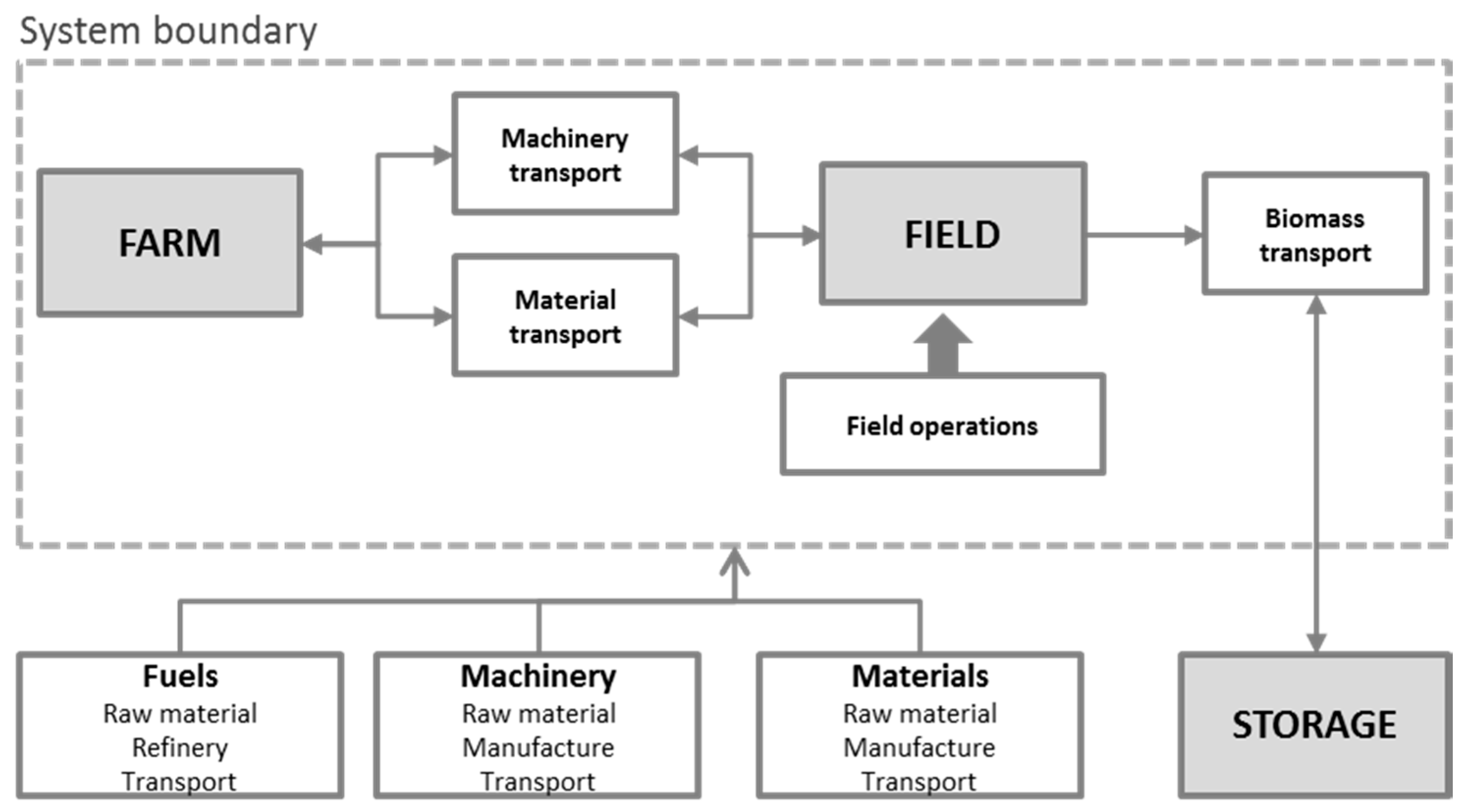
Figure 2.
Core design of the estimation process.

Figure 3.
Energy consumption per crop per field operation (for 10 years cycle) (MJ·ha−1).

Figure 4.
Fuels energy consumption per crop per field operation (for 10 years cycle) (MJ·ha−1).
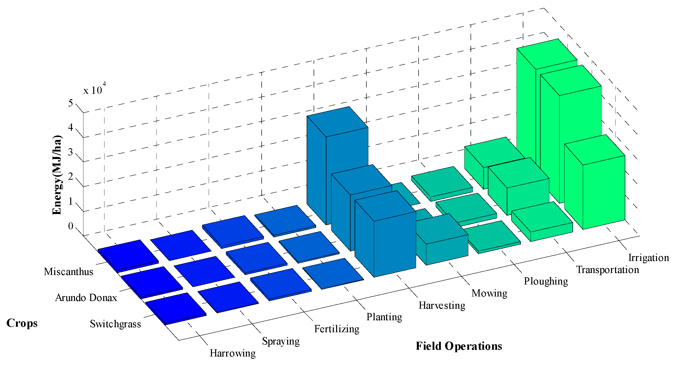
Figure 5.
Embodied energy consumption per crop per field operation (for 10 years cycle) (MJ·ha−1).

Figure 6.
Input energy distribution in MJ·ha−1 for the three crops per 10 years cycle.

Figure 7.
Efficiency of Energy variance in different distances from farm and storage facilities.


Table 1.
Field operations of the three crops for a ten-year period.
| Field Operation | Year | |||||||||||||||||||||||||||||
|---|---|---|---|---|---|---|---|---|---|---|---|---|---|---|---|---|---|---|---|---|---|---|---|---|---|---|---|---|---|---|
| 1 | 2 | 3 | 4 | 5 | 6 | 7 | 8 | 9 | 10 | |||||||||||||||||||||
| C1 | C2 | C3 | C1 | C2 | C3 | C1 | C2 | C3 | C1 | C2 | C3 | C1 | C2 | C3 | C1 | C2 | C3 | C1 | C2 | C3 | C1 | C2 | C3 | C1 | C2 | C3 | C1 | C2 | C3 | |
| Plowing | ● | ● | ● | ○ | ○ | ○ | ○ | ○ | ○ | ○ | ○ | ○ | ○ | ○ | ○ | ○ | ○ | ○ | ○ | ○ | ○ | ○ | ○ | ○ | ○ | ○ | ○ | ○ | ○ | ○ |
| Disk-harrow | ● | ● | ● | ○ | ○ | ○ | ○ | ○ | ○ | ○ | ○ | ○ | ○ | ○ | ○ | ○ | ○ | ○ | ○ | ○ | ○ | ○ | ○ | ○ | ○ | ○ | ○ | ○ | ○ | ○ |
| Agrochemical spreading | ● | ○ | ● | ○ | ○ | ● | ○ | ○ | ● | ○ | ○ | ○ | ○ | ○ | ○ | ○ | ○ | ○ | ○ | ○ | ○ | ○ | ○ | ○ | ○ | ○ | ○ | ○ | ○ | ○ |
| Planting/Seeding | ● | ● | ● | ○ | ○ | ○ | ○ | ○ | ○ | ○ | ○ | ○ | ○ | ○ | ○ | ○ | ○ | ○ | ○ | ○ | ○ | ○ | ○ | ○ | ○ | ○ | ○ | ○ | ○ | ○ |
| Fertilization | ● | ● | ● | ● | ● | ○ | ● | ● | ● | ● | ● | ● | ● | ● | ● | ● | ● | ● | ● | ● | ● | ● | ● | ● | ● | ● | ● | ● | ● | ● |
| Mowing | ○ | ○ | ○ | ○ | ○ | ● | ○ | ○ | ● | ○ | ○ | ● | ○ | ○ | ● | ○ | ○ | ● | ○ | ○ | ● | ○ | ○ | ● | ○ | ○ | ● | ○ | ○ | ● |
| Harvesting | ○ | ○ | ○ | ● | ● | ● | ● | ● | ● | ● | ● | ● | ● | ● | ● | ● | ● | ● | ● | ● | ● | ● | ● | ● | ● | ● | ● | ● | ● | ● |
| Irrigation | ● | ● | ● | ● | ● | ● | ● | ● | ● | ● | ● | ● | ● | ● | ● | ● | ● | ● | ● | ● | ● | ● | ● | ● | ● | ● | ● | ● | ● | ● |
| Biomass transport | ○ | ○ | ○ | ● | ● | ● | ● | ● | ● | ● | ● | ● | ● | ● | ● | ● | ● | ● | ● | ● | ● | ● | ● | ● | ● | ● | ● | ● | ● | ● |
C1: Miscanthus, C2: Arundo donax, and C3: Switchgrass. ●: Applied operation, ○: Non-applied operation.
Table 2.
Field Machinery Inputs.
| Operations | Operating Width 1 (m) | Operating Speed 2 (km·h−1) | Field Efficiency 2 | Tractor Embodied Energy 3 (MJ·kg−1) | Implement Embodied Energy 3 (MJ·kg−1) | Tractor Weight 4 (103 kg) | Implement Weight 1 (103 kg) | Tractor Estimated Life 2 (103 h) | Implement Estimated Life 2 (103 h) | Fuel Energy Content 4,5 (MJ·L−1) | Tractor Power (kW) | Lubricants Energy Content 6 (MJ·L−1) |
|---|---|---|---|---|---|---|---|---|---|---|---|---|
| Plough | 3 | 7 | 0.85 | 138 | 180 | 6.76 | 2.30 | 16 | 2 | 41.2 | 120 | 46 |
| Disk-harrow | 4.5 | 10 | 0.80 | 138 | 149 | 6.76 | 1.80 | 16 | 2 | 41.2 | 120 | 46 |
| Agrochemical Spreading | 24.4 | 11 | 0.70 | 138 | 129 | 2.93 | 3.35 | 12 | 1.2 | 41.2 | 50 | 46 |
| Fertilization | 24.4 | 11 | 0.70 | 138 | 129 | 2.93 | 3.35 | 12 | 1.2 | 41.2 | 50 | 46 |
| Planting/Seeding | 3.15 | 9 | 0.65 | 138 | 133 | 2.93 | 1.20 | 12 | 1.5 | 41.2 | 50 | 46 |
| Mowing | 3.1 | 11 | 0.80 | 138 | 110 | 6.76 | 0.65 | 12 | 2 | 41.2 | 120 | 46 |
| Harvesting | 1.83 | 5 | 0.70 | 138 | 116 | 6.76 | 0.90 | 16 | 2.5 | 41.2 | 120 | 46 |
| Transport | - | - | - | - | - | 6.76 | - | 12 | - | 41.2 | 120 | 46 |
Table 3.
Transportation Inputs.
| Operations | Average Road Speed (km·h−1) | Tanker/Wagon Weight (kg) | Tanker/Wagon Embodied Energy (MJ·kg−1) | Tanker/Wagon Estimated Life 1 (103 h) | Fuel Road Consumption 2 (L·km−1) | Wagon Full Volume 2 (m3) |
|---|---|---|---|---|---|---|
| Plough | 20 | - | - | - | 0.71 | - |
| Disk-harrow | 20 | - | - | - | 0.71 | - |
| Agrochemical Spreading | 20 | 1500 | 108 | 3 | 0.188 | - |
| Fertilization | 20 | 6800 | 108 | 3 | 0.188 | - |
| Planting/Seeding | 20 | 2500 | 108 | 3 | 0.188 | - |
| Mowing | 20 | - | 108 | 3 | 0.71 | - |
| Harvesting | 20 | - | 108 | 3 | 0.71 | - |
| Transport | 20 | 14,500 | 108 | 3 | 0.71 | 40 |
1 [28], 2 Commercial Values.
Table 4.
Irrigation Inputs.
| Lift (m) | Irrigation Useful Life 1 (Years) | PVC Pipe Embodied Energy 2 (MJ·kg−1) | Efficiency | Electricity Energy Coefficient 3,4 (MJ·KWh−1) | ||||
|---|---|---|---|---|---|---|---|---|
| Well | Drip Irrigation | System | Pump 1 | Driving 1 (Electric Motors) | Irrigation System | |||
| 10 | 21 | 3 | 20 | 110.66 | 0.70 | 0.80 | 0.70 | 8.1 |
Table 5.
Energy consumption per field operation for ten years production cycle.
| Field Operation | Crops | Energy Consumption (MJ·ha−1) | |||
|---|---|---|---|---|---|
| Fuel | Embodied | Material | Total | ||
| Ploughing | Miscanthus | 1616 | 281 | - | 1904 |
| Arundo donax | 1616 | 205 | - | 1827 | |
| Switchgrass | 954 | 151 | - | 1109 | |
| Disk-harrowing | Miscanthus | 949 | 152 | - | 1105 |
| Arundo donax | 785 | 120 | - | 909 | |
| Switchgrass | 785 | 120 | - | 908 | |
| Agrochemicals Spreading | Miscanthus | 91 | 73 | 18,160 | 18,326 |
| Arundo donax | - | - | - | - | |
| Switchgrass | 329 | 167 | 4189 | 4624 | |
| Planting/Seeding | Miscanthus | 571 | 135 | 69 | 779 |
| Arundo donax | 444 | 276 | 69 | 800 | |
| Switchgrass | 315 | 80 | 20 | 419 | |
| Fertilization | Miscanthus | 1094 | 1965 | 48,869 | 51,951 |
| Arundo donax | 932 | 1304 | 80,640 | 82,894 | |
| Switchgrass | 1004 | 1409 | 48,415 | 50,847 | |
| Mowing | Miscanthus | - | - | - | - |
| Arundo donax | - | - | - | - | |
| Switchgrass | 8749 | 832 | - | 9621 | |
| Harvesting | Miscanthus | 35,822 | 1856 | - | 37,793 |
| Arundo donax | 22,878 | 1975 | - | 24,934 | |
| Switchgrass | 22,878 | 1004 | - | 23,954 | |
| Irrigation * | Miscanthus | 43,740 | 8202 | - | 51,942 |
| Arundo donax | 43,740 | 8202 | - | 51,942 | |
| Switchgrass | 26,244 | 9322 | - | 35,566 | |
| Biomass transport | Miscanthus | 8771 | 27,041 | - | 39,639 |
| Arundo donax | 11,060 | 33,127 | - | 45,683 | |
| Switchgrass | 3897 | 6272 | - | 13,469 | |
* In irrigation there is electricity consumption instead of fuels.
Table 6.
Energy results.
| Crops | EI (GJ) | EO (GJ) | EIU (GJ·ha−1) | EOU (GJ·ha−1) | EoE | EB (GJ·ha−1) |
|---|---|---|---|---|---|---|
| Miscanthus | 203.4 | 3229 | 203.4 | 3229 | 15.87 | 3025.3 |
| Arundo donax | 209.0 | 4863 | 209.0 | 4863 | 23.27 | 4654.4 |
| Switchgrass | 140.5 | 1900 | 140.5 | 1900 | 13.52 | 1760.3 |
© 2017 by the authors. Licensee MDPI, Basel, Switzerland. This article is an open access article distributed under the terms and conditions of the Creative Commons Attribution (CC BY) license (http://creativecommons.org/licenses/by/4.0/).
Share and Cite
MDPI and ACS Style
Rodias, E.; Berruto, R.; Bochtis, D.; Busato, P.; Sopegno, A. A Computational Tool for Comparative Energy Cost Analysis of Multiple-Crop Production Systems. Energies 2017, 10, 831. https://doi.org/10.3390/en10070831
AMA Style
Rodias E, Berruto R, Bochtis D, Busato P, Sopegno A. A Computational Tool for Comparative Energy Cost Analysis of Multiple-Crop Production Systems. Energies. 2017; 10(7):831. https://doi.org/10.3390/en10070831
Chicago/Turabian StyleRodias, Efthymios, Remigio Berruto, Dionysis Bochtis, Patrizia Busato, and Alessandro Sopegno. 2017. "A Computational Tool for Comparative Energy Cost Analysis of Multiple-Crop Production Systems" Energies 10, no. 7: 831. https://doi.org/10.3390/en10070831
Note that from the first issue of 2016, this journal uses article numbers instead of page numbers. See further details here.