
Applicability of an Artificial Neural Network for Predicting Water-Alternating-CO2 Performance


Department of Energy Resources Engineering, Inha University, Incheon 402-751, Korea
*
Author to whom correspondence should be addressed.
Energies 2017, 10(7), 842; https://doi.org/10.3390/en10070842
Submission received: 2 April 2017
/
Revised: 9 May 2017
/
Accepted: 10 May 2017
/
Published: 24 June 2017
Abstract
:The injection of CO2 as part of the water-alternating-gas (WAG) process has been widely employed in many mature oil fields for effectively enhancing oil production and sequestrating carbon permanently inside the reservoirs. In addition to simulations, the use of intelligent tools is of particular interest for evaluating the uncertainties in the WAG process and predicting technical or economic performance. This study proposed the comprehensive evaluations of a water-alternating-CO2 process utilizing the artificial neural network (ANN) models that were initially generated from a qualified numerical data set. Totally two uncertain reservoir parameters and three installed surface operating factors were designed as input variables in each of the three-layer ANN models to predicting a series of WAG production performances after 5, 15, 25, and 35 injection cycles. In terms of the technical view point, the relationships among parameters and important outputs, including oil recovery, CO2 production, and net CO2 storage were accurately reflected by integrating the generated network models. More importantly, since the networks could simulate a series of injection processes, the sequent variations of those technical issues were well presented, indicating the distinct application of ANN in this study compared to previous works. The economic terms were also briefly introduced for a given fiscal condition which included sufficient concerns for a general CO2 flooding project, in a range of possible oil prices. Using the ANN models, the net present value (NPV) optimization results for several specific cases apparently expressed the profitability of the present enhanced oil recovery (EOR) project according to the unstable oil prices, and most importantly provided the most relevant injection schedules corresponding with each different scenario. Obviously, the methodology of applying traditional ANN as shown in this study can be adaptively adjusted for any other EOR project, and in particular, since the models have demonstrated their flexible capacity for economic analyses, the method can be promisingly developed to engage with other economic tools on comprehensively assessing the project.
1. Introduction
Because large volumes of crude oil are normally left underground after primary and secondary production phases and oil prices have remained low, enhanced oil recovery (EOR) technology has attracted more interest recently to produce more profit before field abandonment [1]. Generally, thermal recovery, chemical flooding, and gas flooding are most commonly utilized. However, the most effective methods primarily depend on diverse factors, such as reservoir characterization, operation conditions, fluid properties, and most importantly, economic conditions. Theoretically, the thermal method is suitable for heavy oil as it reduces oil viscosity and makes crude oil moveable. Chemical flooding involves the injections of surfactants, alkalis, and polymers to reduce the interfacial tension (IFT) between oil and water to an ultra-low value and improve sweep efficiency as a result of controlling the displacing fluid mobility by increasing viscosity [2]. Gas flooding is applied to reservoirs still close to production as the injected gas can be recycled from the producing gas. Reusing CO2 from anthropogenic sources is globally incentivized, and gains the dual benefit of EOR and carbon storage, known as carbon capture and storage (CCS) in the petroleum industry [3]. Not only utilized in the petroleum industry, the larger scope of carbon application, defined by the Research Coordination Network as carbon capture, utilization, and storage (CCUS), consists of all methods and technologies for removing CO2 from the emitted gas and atmosphere, followed by recycling this CO2 for use and determining safe and permanent sequestration options. Compared to chemical flooding, the injection of CO2 is much less expensive in terms of fluid employment if sufficient CO2 is available; however, relevant designs for injection are still in dispute owing to the inevitable low sweep efficiency after gas breakthrough or improper carbon storage caused by gas leakage. Due to these ongoing issues, it is important to verify the comprehensive performance of gas flooding for EOR projects with various injection designs and different reservoir characteristics. Furthermore, because CO2 storage underground is encouraged to reduce atmospheric greenhouse carbon, which is represented by an incentive tax credit, balancing the dual benefit (environment and oil production) needs to be prudently considered in any project.
Injected CO2 significantly reduces oil viscosity, swells trapped oil droplets, and finally mobilizes oil. In particular, CO2-EOR has been demonstrated to increase oil mobility quickly when the complete capillary number lies in the immediate range [4]. CO2 can be miscible or immiscible with crude oil depending on reservoir pressure; however, asphaltene depositions that inevitably occur in a reservoir can be problematic due to wettability alterations or formation plugging, lowering the ultimate oil recovery as a consequence [5]. When reservoir pressure is higher than the minimum miscibility pressure (MMP), the gas flooding miscibility scheme is guaranteed due to gas condensation, vaporization, or both of these driving processes. Because miscible flooding has been proven to outperform the immiscible flooding scheme [6], pressure changes in the reservoir should be continuously monitored to ascertain the flooding processes and suitably adjust the operating conditions [7]. Ren et al. proposed a microseismic monitoring program that has been successfully applied in the Jilin oilfield in China to trace the anisotropic flow of CO2 and forecast the oil sweep efficiency of the flooding processes [8]. According to the map created using this method, the obtained carbon migration in the thin layer and essential profiles are in good agreement with CO2 production and the reservoir’s petrophysical properties. In addition to pressure, other important reservoir characteristics, such as depth, permeability, and scaling features need to be prudently addressed in order to efficiently deploy an EOR project either technically or economically [9,10]. An example from the Yanchang oilfield has demonstrated the limited application of CO2 flooding and storage for some depleted reservoirs; only 8 of 27 oil pools had the capacity to enhance oil production using CO2-EOR processes with a storage coefficient of 0.185 [11]. Among the technologies for CO2 injection, the water-alternating-gas (WAG) scheme appears to be most effective for controlling the mobility of the injected fluid as water and gas are alternated in cycles [12,13]. However, Song et al. indicated that technical improvements in the WAG process decline when the pay thickness is over 30 m [14]. From a well pattern aspect, they also confirmed that a five-spot pattern is more effective in carrying out a WAG project compared to the inverted nine-spot or inverted seven-spot patterns. Once the reservoir characterizations and proper well installations have been addressed, the fiscal term needs to be prudently examined as critical performance strongly depends on oil price, CO2 cost, project life, and other economic factors [15].
In most EOR projects, estimation issues are always a concern in minimizing risk and maximizing production from either technical or economic perspectives. Ettehadtavakkol et al. [16] proposed a screening tool to optimize two problem categories: fixed storage requirement and integrated asset optimization. Promisingly, the suggested workflow can powerfully rank CO2-EOR candidates for oilfield operators and governments. Ahmadi generated an artificial neural network (ANN) to predict asphaltene precipitation in reservoirs under certain conditions. With a coefficient of determination larger than 0.996, the model can be potentially combined with other software to speed up performance and increase prediction capacity [17]. By applying the response surface methodology integrated with Monte Carlo simulations, Pan et al. [18] forecast and evaluated the uncertainty in cumulative oil production, net CO2 storage, net water stored, and reservoir pressure at injection wells in different injection and reservoir scenarios based on changing anisotropic permeability, WAG time ratio, and initial oil saturation. An integrated framework developed by Dai et al. [19] also analyzed the response surface for water-oil flow reactive transport to study the sensitivity and optimization of CO2-EOR performance. They concluded that reservoir parameters, such as depth, porosity, and permeability are crucial to control net CO2 storage, while well distance and the sequence of alternating water and CO2 injection are significant operational parameters for process design. A newly developed intelligence tool was introduced by Eshraghi et al. [20] for optimizing the miscible CO2 flooding process in terms of inter-well characterization by employing a capacitance-resistance model coupled with Gentil fractional flow. From three heuristic optimization methods, they verified the predominant performance similarity to an artificial bee colony for particle swarm optimization and genetic algorithm methods to predict well transmissibility.
Understanding the relevant applications of the ANN model, this study attempts to generate and justify neural networks for different targets to compute the output at multiple points of a WAG process. Two reservoir parameters and three surface operation factors were designed as input parameters, and three critical performances at 5, 15, 25 and 35 injection cycles were included in the output layer of each ANN model. Because the networks have been successfully achieved, technical relationships among parameters and optimizations were also evaluated to justify the quality of these models. The economic aspects of the project are also evaluated using the net present value (NPV), which also demonstrates the applicability of the networks. Generally, the generated networks can be employed in other cases with similar site characteristics; in particular, the method using ANN can be used in other research areas for different predictive purposes.
2. 3D Model Characteristics
2.1. Reservoir Descriptions
A 3D reservoir is modeled in GEM (CMG) (2016, Computer Modelling Group Ltd., Calgary, AB, Canada) with a five-spot well pattern scale in which the reservoir characteristics are referenced from the Morrow sandstone formation at the Farnsworth EOR target field [18]. The reservoir model is set with a constant depth of the top layer at 2362 m and a pay thickness of 9.15 m, which originated from the average depth and net pay at the Farnsworth field [21]. Other reservoir properties are presented in Table 1; porosity and horizontal permeability are heterogeneous over the reservoir with a nearly tenfold change between minimum and maximum values. Vertical permeability is represented by the permeability ratio Kv/Kh, and an equal-distance between each injection and producing well is assigned as an input variable in the network model. Water saturation and reservoir pressure are uniformly set over the model domain; this is suitable for initialization, as the initial water saturation is also assigned as a neuron metric in the ANN.
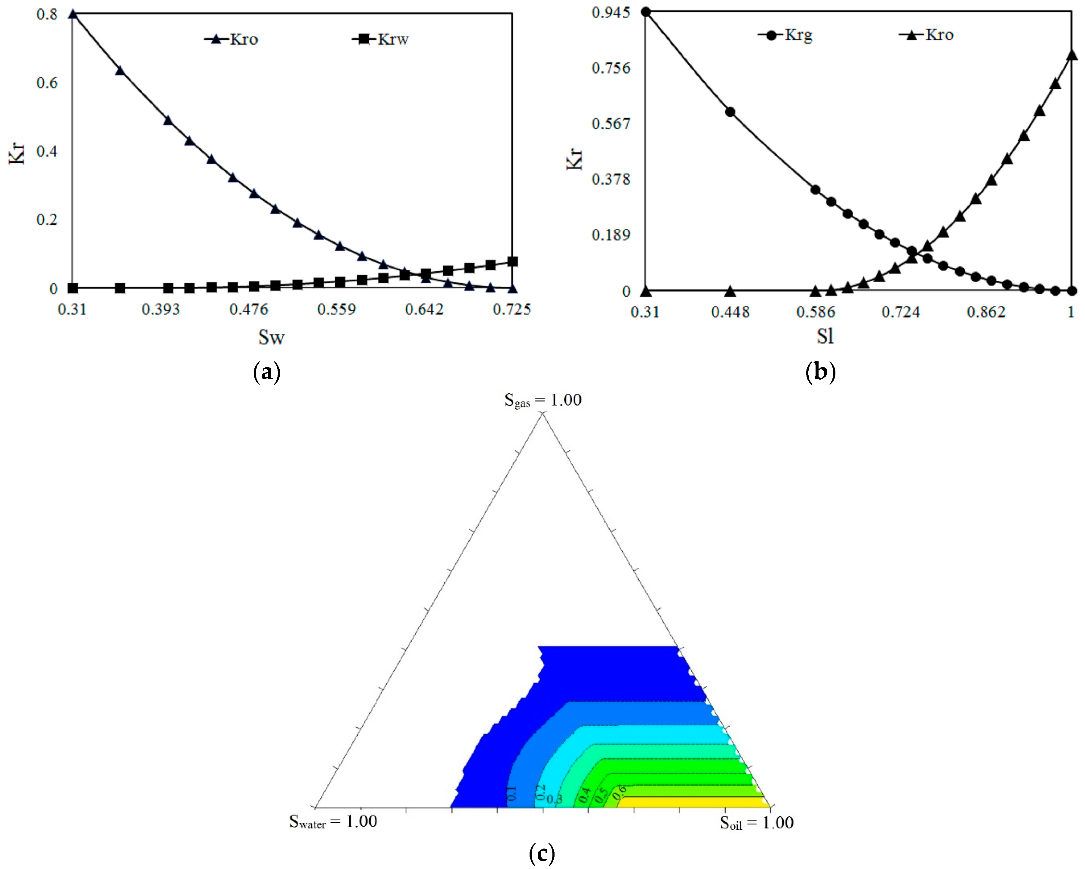
Because the critical CO2 condition is at 7.384 MPa and 31.1 °C, the reservoir condition is appropriate for consideration as a carbon capture project because it always exists at the super critical phase when injected into the reservoir. Dip angle usually occurs in most practical fields, and it partially affects the movement of the injected gas due to gravity [22], but this factor is not considered in this model. Salinity is also neglected in the CO2 injection process, as its influence on solubility is negligible. The permeability curves for oil-water and liquid-gas in this rock system are shown in Figure 1 [7].
2.2. Fluid Properties
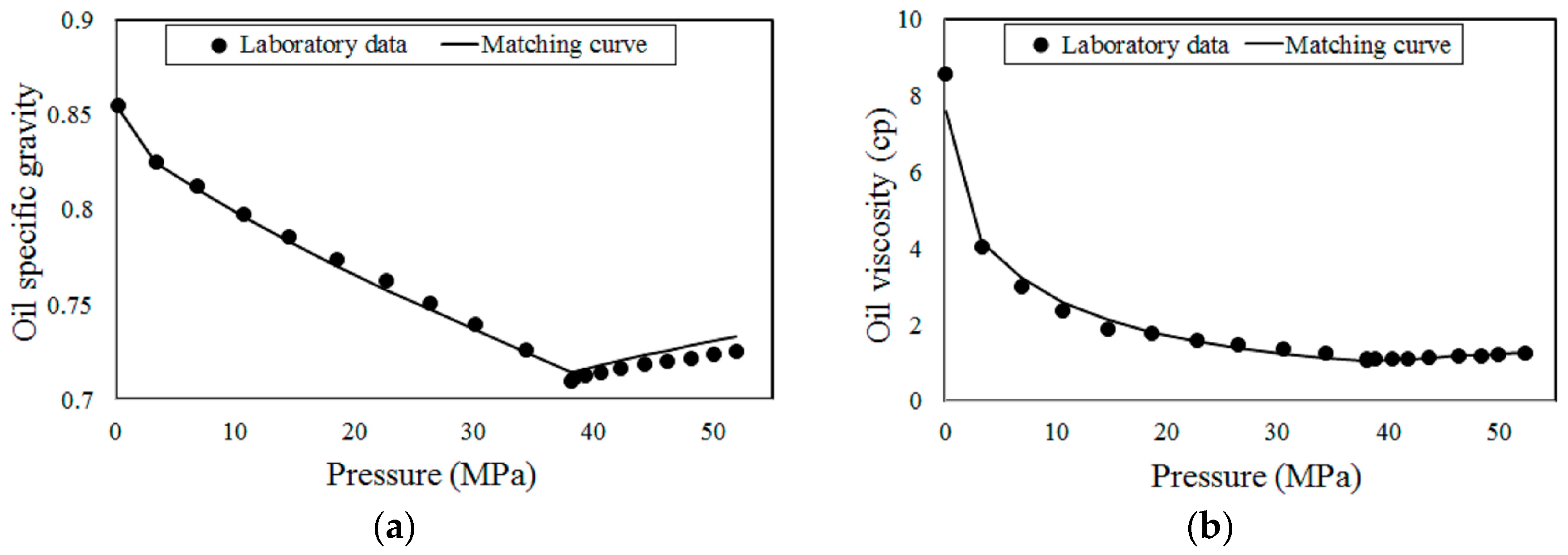
In total, nine pseudo-hydrocarbon and non-hydrocarbon components of a referenced crude oil are verified in WINPROP (CMG) to validate PVT testing data from laboratory measurements, as shown in Table 2. The full, original components can be obtained from the literature [23]. The oil specific gravity, gas oil ratio, oil viscosity, and oil formation volume factor are primarily measured in a differential liberation test (DLT), while CO2 is assigned as the secondary component in a swelling test (ST). The regression for all testing data is made on the basis of the Peng-Robinson equation of state [24]:
where p, R, T, and v represent pressure, constant factor, temperature, and volume, respectively, and a and b are calculated in terms of the critical properties and acentric factor as follows:
With and .
where α is an acentric factor, pc and Tc are the critical pressure and temperature, respectively, while parameters and are constants with and . Because the swelling test regression has been accounted for in the simulation, multiple contact behaviors are then computed in order to determine the MMP for CO2 and crude oil. Theoretically, there are some effective methods integrated in the simulator to calculate MMP such as cell-to-cell, semi-analytical (key tie lines), and multiple mixing cell methods. The traditional cell-to-cell method generates a pseudo-ternary diagram from computations to help with interpreting results. In the semi-analytical method, the MMP is determined based on the point that one of three key tie lines is tangent to the critical locus, and the crossover tie line controls the development of miscibility [25,26]. A more simple but effective method proposed by Ahmadi and Johns, known as the multiple mixing cell, also focuses on key tie lines, but instead of finding all key tie lines, MMP can be determined by tracking only the shortest one [27]. As the final method is robust, the most accurate, and more stable than the others, this study uses it to calculate the MMP for the CO2 injection process on the given crude oil.
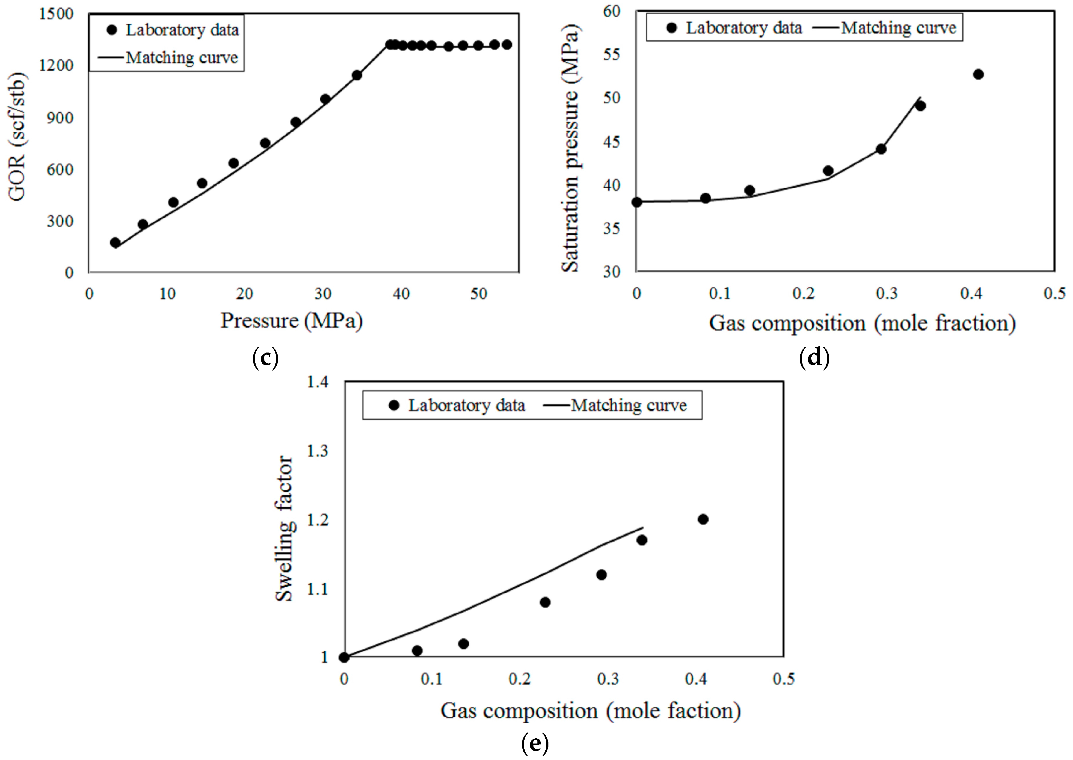
The results of matching the given laboratory data for critical crude oil properties are presented in Figure 2. First, the differential liberation testing (DLT) data match very well under the regression scheme based on the Peng-Robinson equation of state, indicating the successful PVT analysis simulation for the given crude oil and guaranteeing that the hydrocarbon properties are identical to the testing data in the 3D dynamic simulation. Second, as illustrated in the figure, saturation pressure points are excellently matched in the swelling test (ST) (CO2 was used as a secondary component), while there are small deviations on swelling factor points. However, technically, the deviations are acceptable, so the numerical transformations of hydrocarbon components caused by CO2 injection can be approved for further processes. The MMP value is also predicted using the above-mentioned multiple mixing-cell method with a starting pressure at 3.4 MPa. The prediction shows that multiple contact miscibility can be achieved from 18.92 MPa under a back-forward condensing gas drive, much less than the reservoir pressure. Therefore, the EOR will be under a miscible flooding scheme during the injection process in the reservoir [28].
3. Neural Network Model Generation
Multiple WAG cycles initialized by a water injection are designed for simulations. The producing well is constrained with a minimum bottom hole pressure at 13.79 MPa. The four injection wells have the same constraints, with maximum injection rates for water and CO2 at surface conditions. In detail, water will be injected at 86.36 m3/day and cycled with CO2 injection at 5435.57 sm3/day. The well operation conditions are unchanged during the simulation processes. The well distance between each injector and producer (hereafter D) is considered from 200 m to 400 m at the same reservoir scale. Technically, increased spacing between injection and producing wells helps postpone the gas breakthrough, improve diffusion of gas in the reservoir, and store larger quantities of carbon underground. However, inappropriately-long well distances reduce the amount of produced gas that can be re-injected into the reservoir, and increases the cost of purchasing CO2. The WAG ratio is defined as the cumulative continuous CO2 injection time divided by that of water in an injection cycle and varies from 0.5 to 3.5 as a critical factor in the neural network model. Fundamentally, the increase in simultaneous CO2 injection extracts greater quantities of oil from the pore volume in the swept regions, but it also causes early breakthrough, after which both oil production and net CO2 storage are reduced [29]. In contrast, a bias toward water injection significantly decreases the time CO2 is in contact with the hydrocarbon and lowers sweep efficiency as a consequence. Furthermore, because CO2 solubility in water is also taken into consideration in the simulation, an effective WAG ratio should be carefully designed in the process. For the injection scheme, the duration of one cycle (hereafter T) is also considered in the network model, with a variation from 30 days to 90 days. The expression of the WAG ratio and T can fully represent the examination for the WAG injection scheme of the project. The consequences of reservoir characteristics are also verified in the network through vertical permeability and initial water saturation; these two parameters are uncertain and variable in the reservoir. Vertical permeability is represented by the permeability ratio as previously mentioned (Kv/Kh) and varies from 0.1 to 1, while the initial saturation (Sw) ranges from 0.6 to 0.725 in the network model. The consideration of reservoir properties substantially aids in determining the most favorable reservoir capacity for managing a CO2-EOR process in terms of both oil production and net CO2 storage, factors that directly affect the consistency of the injection designed parameters.
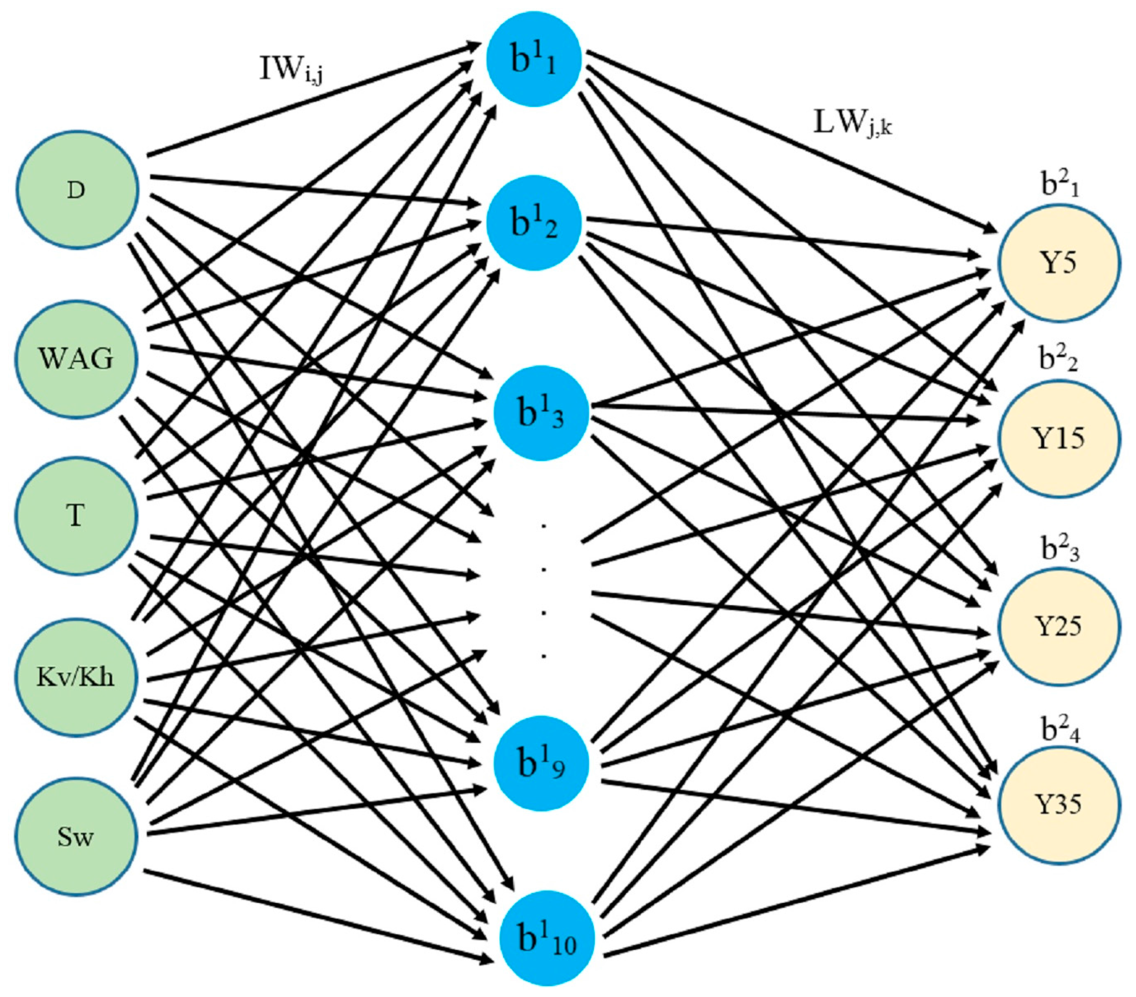
The oil recovery factor, cumulative gaseous CO2 production, and net CO2 storage (in mass) in a reservoir are considered essential targets for flooding performance in the three distinguishable neural networks. In particular, each target will be predicted after a series of injection cycles, including 5, 15, 25 and 35 cycles in a same network, representing four neurons in the output layer of the ANN architecture, as illustrated in Figure 3. There are 10 neurons in a hidden layer of the structure connecting with other forward and backward neurons of input and output layers. Because the sample data set is stable and qualified for training, the design of one hidden layer is suitable and effective for learning purposes, and also simpler to reuse in other spreadsheets.
Systematically, the neurons of each layer connect with neurons of its forward layer and back layer through weights and biases, indicating the contributory level of an individual neuron on the others. As presented in Figure 3, each neuron in the hidden layer is connected to others in the input layer through the activation formula:
where , Xi represents the input components in the input layer (5 neurons), IWi,j is the connection weight between the ith neuron in the input layer and the jth neuron in the hidden layer, and bj1 presents the bias value assigned to the jth neuron in the hidden layer. The tan-sigmoid activation (or transfer) function is defined as:
A similar connection is performed between the jth neuron in the hidden layer and the kth neuron in the output layer through the connection weights, LWj,k as . However, instead of a tag-sigmoid function, a linear link is introduced for the final transfer function to connect each kth neuron with the bias bk2 in the output layer. To avoid the effect of large values on small values during training, normalization is introduced for all data points prior to the training process as follows:
where X represents the normalized data points inserted in the training process, while Xsam, Xmin, and Xmax are real sample data values; lower and upper constraints of these real data correspond to design variables and targets, respectively. Theoretically, normalization helps support the training process and does not affect the final results because all data will be easily converted to real values according to the formula. As mentioned previously, a large range of values for each designed parameter has been proposed, and broad differences between resulting targets can be achieved for further evaluation.
4. Results and Discussion
4.1. Simulation Results
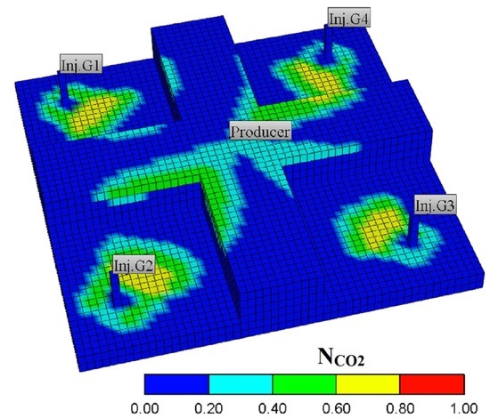
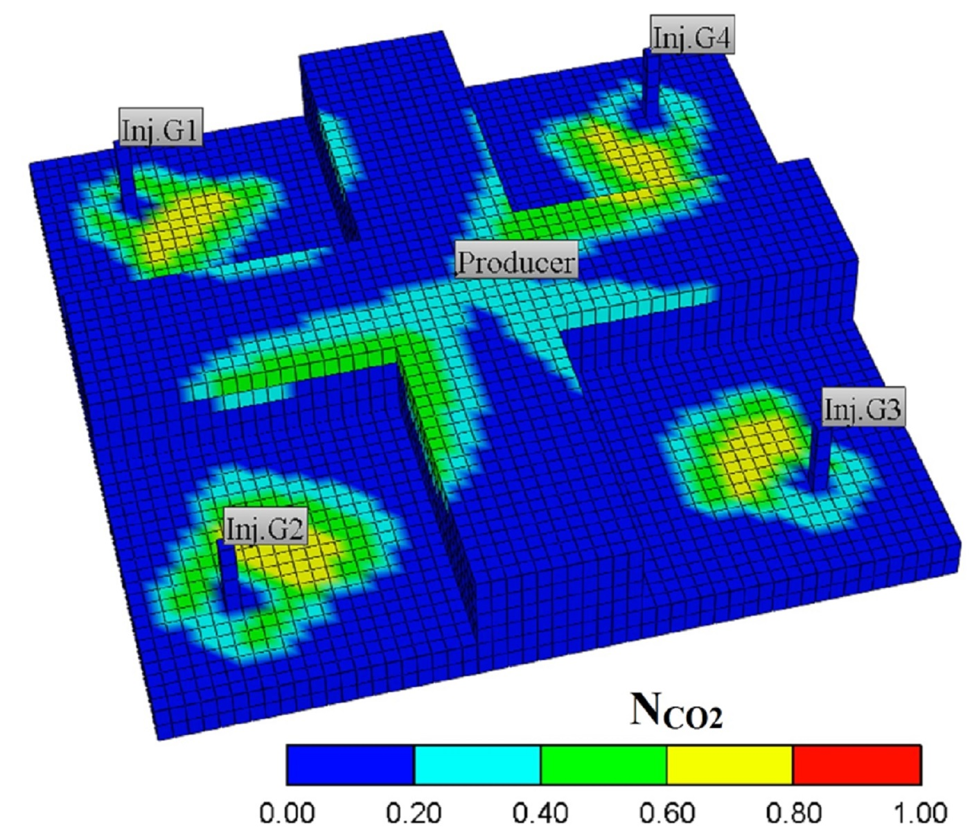
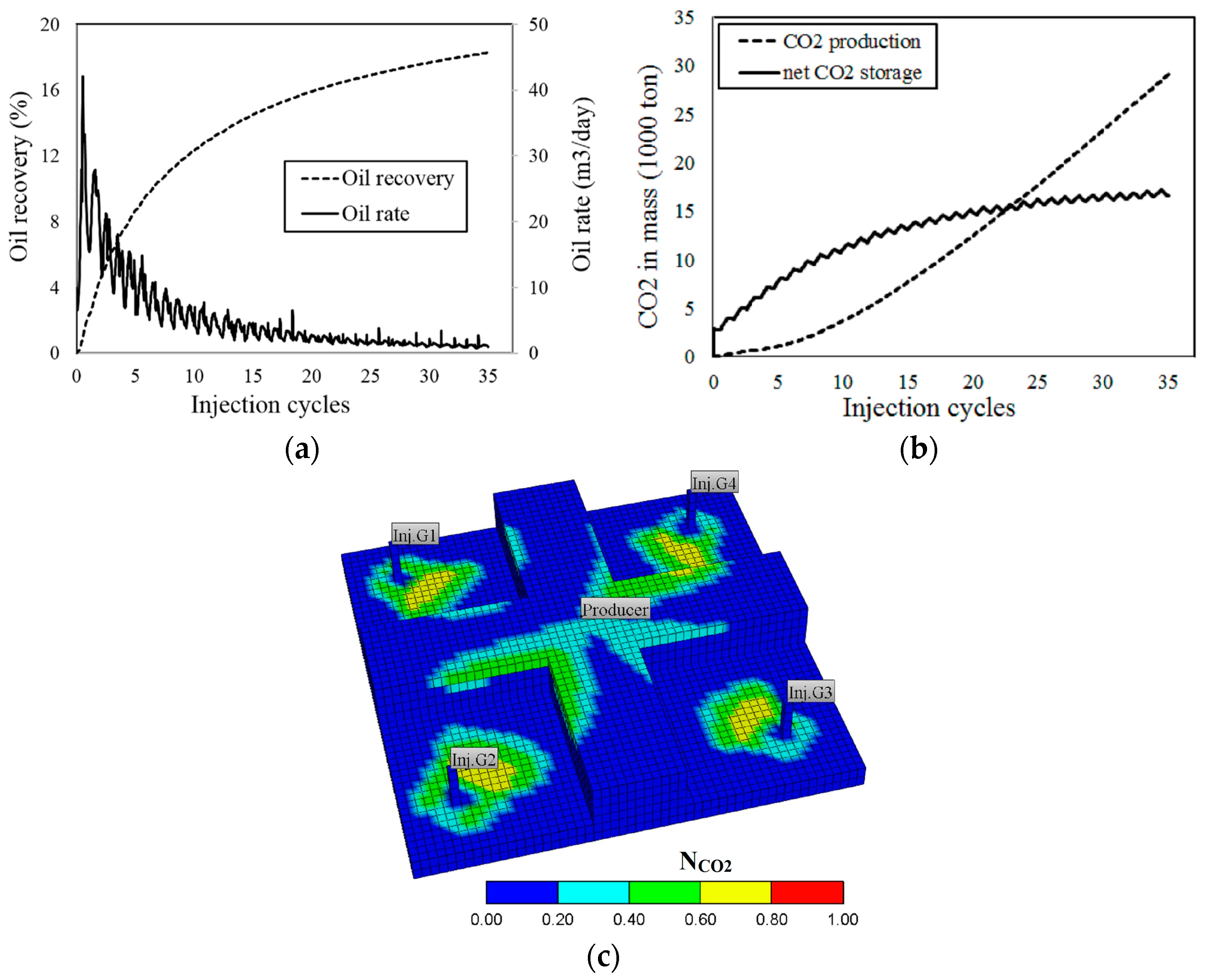
The results of the first simulation should be validated first in terms of physically dynamic performances before analyzing further procedures. The case is designed with an equal injection time for water and gas in each 60 days of a single cycle for a well distance of 300 m in the pattern. The initial water saturation and permeability ratio are respectively set to 0.67 and 0.5 for this case. Subsequently, critical performances will be evaluated after 300, 900, 1500, and 2100 days of injection since initiation, corresponding to 5, 15, 25 and 35 cycles, respectively. These performances are shown in Figure 4.
As presented in Figure 4, approximately 22.5% oil in place (OIP) is recovered after 25 cycles and an increment of nearly 1% after 10 more injection cycles. Practically, this oil recovery factor result is acceptable compared to simulations processed for other real projects [30]. The gas breakthrough time can be visualized through the change in slope of the net CO2 storage or cumulative gas production. Subsequently, gas breakthrough occurs prior to an additional 10 injection cycles; more precisely, it is within the 5th cycle of flooding. This is confirmed in the profile of the global CO2 mole fraction after 5.5 injection cycles, as detected through the earliest approach of CO2 into the producing well. Even though the unexpected gas breakthrough has been observed, the CO2 flow profile is obviously impacted by gravity effects based on the large difference in CO2 concentration between the bottom and top layers, causing a non-uniform swept area. The small increases in net CO2 sequestration after 15 cycles indicate that CO2 storage has reached the highest capacity in the reservoir. Generally, these crucial performance criteria can be improved by adjusting the injection scheme, such as the WAG ratio or maintenance time of each cycle for a specific reservoir condition [31].
4.2. Neural Network Model Evaluations
In total, 263 simulation samples are collected for generating four ANN models. The results present diversity in the critical objectives after each specific assigned injection cycle. As shown in Figure 5, the ultimate oil recovery ranges from around 2% to less than 30% OIP; in some cases, the recovery factor (RF) can be up to 18% after 5 cycles. However, oil recoveries do not improve considerably from 25 to 35 cycles. The total amount of CO2 stored underground is unpredictable after 15 cycles, as it might decline or increase at 25 and 35 injection cycles, while the gas produced rises continuously from the beginning of the process. Generally, the more complicated and diverse sample results correspond to higher levels of representation achieved from successful models used for estimation.
Using the MATLAB Network Toolbox, the ANN model for the previously described performances is trained following a 50%-20%-30% training scheme corresponding to the percentage ratio of data used for the training validation test in the 263 numerical samples. More specifically, the generated model from training is automatically applied to estimate 79 random blind data (30%) to ensure the avoidable over-training phenomenon. The same training scheme is applied to the three different targets, but the specific data points for the training processes, corresponding to dissimilar networks, are selected differently owing to non-concurrent training. Mathematically, neural networks are trained under a feed forward back propagation algorithm in which weights and biases are initially allocated in the structure. Neurons in the output layer are first calculated based on the initial structure; an adjustment is made for weights and biases thereafter based on errors between sampling and current computed targets. These forward and backward computations are performed during training until the lowest overall errors are obtained. The over-training phenomenon can occur in an unsuitable training scheme ratio. Therefore, a higher percentage of data points used for blind testing assures more confidence in the quality of the training and generated model.
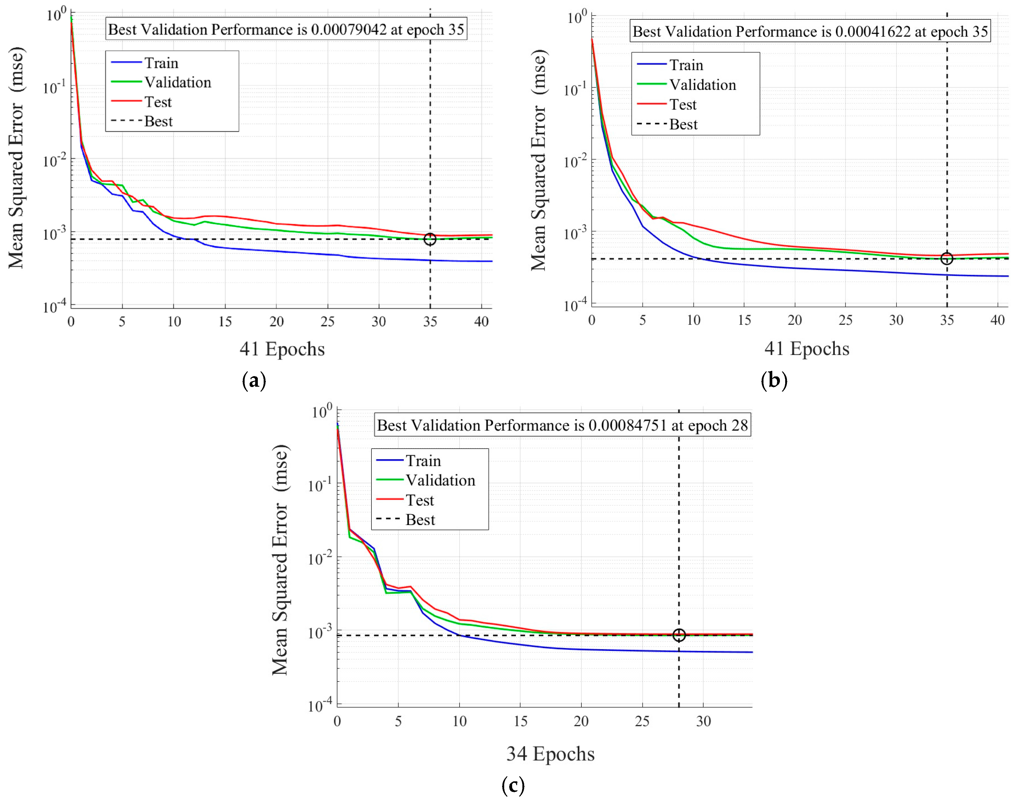
Figure 6 shows the training performances of the three crucial objectives based on the number of epochs and mean square errors during training. Principally, a successful training is only accomplished when the best standing points correspond to the lowest errors in the validation, and test curves are not very different in terms of the epoch number. Subsequently, all final training performances are definitely qualified as optimized points in both validation and test curves when they are sufficiently close to each other, with errors less than 0.001. The reasonably low errors in training presumably indicates the high accuracy of the ANN models for forecasting targets for any input values within their constraints. Indeed, the recomputed targets for the sample data show good agreement with the simulation results in Figure 7, and the blind test data are also excellently matched during the injection processes.
The quality of estimations is evaluated quantitatively using two decisive factors, known as the coefficient of determination (R2) and the root mean square error (RMSE) from the formulae:
where zi,sam, zi,ANN, and represent data points from the samples, estimation by the network, and average values of the sampling data, respectively. Theoretically, R2 values higher than 0.95 and RMSE values less than 4% for regressions are acceptable for prediction. Therefore, the ANN models are absolutely qualified, with most R2 values higher than 0.98 and RMSE values less than 3.2% in all injection cycles (Table 3). This potentially opens the possibility of extending the number of neurons in the output layer in future work to comprehensively estimate the flooding performance. Because the models have been successfully generated, they can be easily applied to any adequate spreadsheet based on the weights and biases in the network structure.
The values from the three networks are fully presented in Table 4. Mathematically, the neural networks are proven to accurately compute subjective targets within the design variables. However, the technical relationships between variables also should be evaluated to validate the models and determine if there is sufficient sample data coverage.
4.3. Applicability of ANN Models
Conventionally, the oil recovery factor and capacity of carbon sequestration are primarily concerned with CO2 flooding from the technical perspective, while the ultimate profitability is the decisive factor for evaluating the success of the project economically. A large amount of oil production might appear preferable, but as oil prices are unexpectedly low, purchasing CO2 needs to be taken into consideration, particularly when the incentive tax credit is counted according to the total volume of carbon sequestration in the reservoirs. Therefore, competent ANN models should tackle both the technical and economic aspects of the problem.
Favorable reservoir properties are investigated first through initial water saturation and a dimensional permeability ratio at the base case injection and well spacing design. As shown in Figure 8, with a specific operation condition, the permeability ratio impacts the oil production differently according to the injection cycle progress. In detail, after five cycles, this factor seems to have no effect on RF, whereas RF has an inverse relationship with Kv/Kh after 25 injection cycles with a deviation of approximately 5% in RF between the lower and upper permeability ratio thresholds. This confirms that a high difference between vertical and horizontal permeability has an advantage in extracting reservoir oil; reservoirs that have low vertically permeable flow capacity are preferable. Physically, this result can be explained by the gravitational effect, associated with a heterogeneous system, which inevitably occurs while injecting CO2 into the reservoir even though water is also used for cycling.
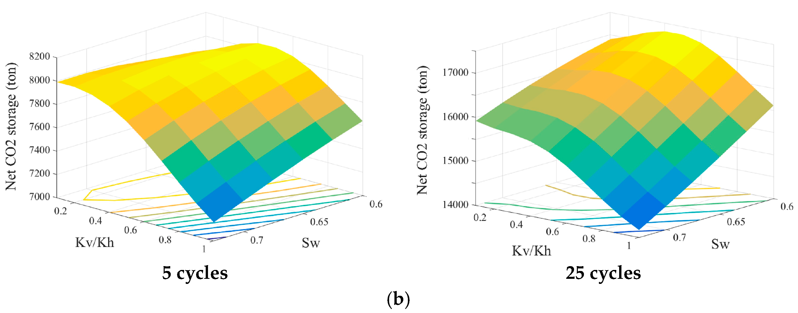
Regarding carbon sequestration, a system having Kv/Kh less than 0.5 proves to be the most advantageous for initial fluid conditions and storing CO2 throughout the flooding process. Principally, the gas can be trapped under various mechanisms in the geological formation, such as mineral trapping, solubility trapping, or residual trapping. In particular, the amount of oil displaced is proportional to the CO2 storage volume in the reservoir. This explains the increase in trapped gas following the decrease in water saturation after either 5 or 25 cycles, as shown in Figure 8. Clearly, the dependence of oil production and net CO2 storage on both reservoir factors implies an identical assessment for potential CO2-EOR using reservoir characteristics.
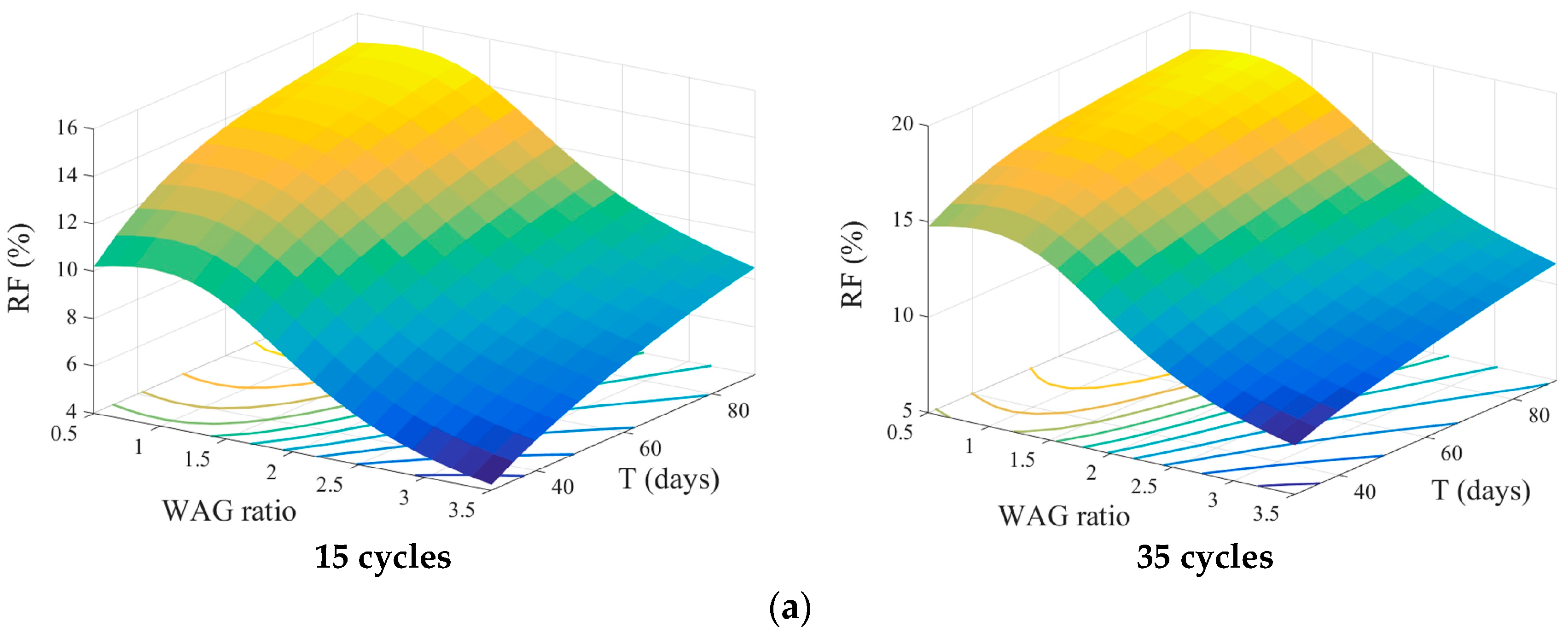
In terms of surface control, the relevant injection designs should also be determined to address dependent performances according to different flooding schemes [32,33,34]. Fundamentally, an appropriate WAG injection design helps extend the contact time between gas and in situ hydrocarbon, mitigating viscous fingering and maximizing thoroughly swept areas. Depending on reservoir properties and initial fluid conditions, optimal designs for injecting gas and water might differ, however the basic technical relationships will presumably be identical for all system properties. Figure 9 illustrates the changes in the three subjective targets following various WAG ratio and duration time T designs, at reservoir conditions Kv/Kh = 0.5 and initial Sw = 0.67. Obviously, an increase in T enhances all targets at dissimilar magnitudes during the injection process, while rising RF and net CO2 storage stop at an optimal WAG ratio region before decreasing according to increases in this parameter. Specifically, WAG ratios around 1 maximize the recovery factor after either 15 or 35 cycles, whereas a ratio of 2:1 for the injection time for CO2 to water is most favorable for gas storage in the formation (Figure 9).
The continuous increase in gas injection might initially extract a significant amount of trapped oil, but it causes an early breakthrough as a result of high mobility. In contrast, unsuitably low WAG ratios do not guarantee sufficient contact between solvent and hydrocarbon due to a rapid overlap by the injected water. As presented, the high RF is only achieved at a low WAG ratio (less than 1.5). Higher ratios up to 3.5 are undesirable as the RF drops by approximately 5% at the upper WAG ratio. This is also clearly indicated by the large gas production profile after 35 cycles and large incremental change from approximately 50,000 tons to more than 80,000 tons corresponding to a WAG ratio increase from 1 to 3.5 (Figure 9). Similarly, inappropriately high WAG ratios undoubtedly lower the amount of CO2 sequestration, demonstrating the CO2 storage limit in the reservoir corresponding to a specific operating condition, particularly when oil is inefficiently displaced by the injected fluids. From the figure, it is clear that the WAG ratio is more important than time T for injection design [35], even though T has a broad range (30 to 90 days).
The effects of well spacing on essential performances should also be examined using the network models. Generally, the longer distance between an injector and producer results in a later time of gas breakthrough observed at the producing well and higher oil volume recovered during the flooding process. However, when the injected fluid ratio (CO2 to water) is sufficiently high, this spatial factor does not have a significant impact on the WAG project success, for both the RF and other critical targets. As clearly shown in Figure 10, with a WAG ratio at 0.5, the ultimate oil recovery can be improved from nearly 12% to 21% corresponding to an increase of 200 m in well distance. The increment is just 10% if the WAG ratio is designed at 3.5. The deviations in the increment for net CO2 storage between these two WAG ratios are also significant, with increases of approximately 5 kt and 13 kt at the upper and lower constraints of the injecting ratio, respectively. Regarding CO2 production, this target is inversely related to well spacing, but is impacted more by the WAG ratio compared to the spatial factor (Figure 10).
The aforementioned technical verifications have validated the ANN models, not only for forecasting mathematically, but also for providing viable evaluations for targets’ behavior with changes in input parameters. Consequently, the models are flexible for other analyses, such as quantitative optimization or economic feasibility studies. To clearly acknowledge these concerns, a specific fiscal condition is assumed in this work, taking into account the important factors for economic analysis. The detailed expenditure components corresponding to the five-spot well pattern are listed in Table 5, as referenced from the literature [15,36]. Among these, the predicted oil prices from 35 $/bbl to 65 $/bbl are investigated; uncertainty in the crude oil market remarkably influences any oil production project. The encouragement for storing CO2 underground is reflected through an additional incentive term. Furthermore, assuming that all CO2 produced is re-injected in addition to the purchased amount, the cost is ~30% less than if all gas is purchased for injection.
In total, six reservoir cases with interchanging Sw (0.6 and 0.7) and Kv/Kh (0.1, 0.5 and 1) are optimized for NPV by selecting the most favorable injection design and well distance. The procedure is a simple iterative scheme in which the variables are divided into intervals within their constraints. In detail, the well distance has an increment of 20 m from 200 m, and the WAG ratio and T are examined in 0.15 and 5 day intervals, respectively. Subsequently, the maximal NPV is chosen for each reservoir case at 25 injection cycles, and the optimal variables are obtained concurrently. Presumably, the optimized results will be different according to reservoir categories, and the maximized profit and recovery factor might not be achieved with the same parameter values.
Indeed, as presented in Table 6, the most dominant well distance and duration time obtained are dissimilar among the six cases, while the most favorable injected fluid ratio is proposed as 0.5 for most cases. It is clear that although the upper threshold of T is suggested for maximum recovery of the crude oil and CO2 storage underground, a parameter value from 30 to 60 days produces the most economic benefit for the project. In addition, despite the fact that the WAG ratio essentially determines the technical success of the flooding process, a lower value is more preferable for project feasibility and profitability. Clearly, positive NPV values show the profitability of this CO2-EOR project after 25 cycles at a specific oil price (45 $/bbl). However, the project needs to be verified in the context of various market forces to aid in scheduling and evaluating the process.
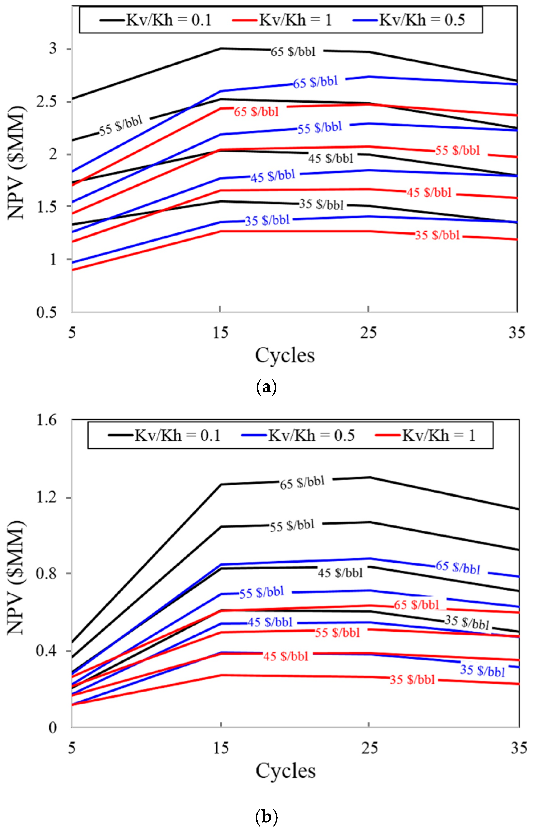
The comprehensive profits for the six cases are illustrated in Figure 11. As described, oil price changes significantly affect the NPV, particularly when reservoir conditions are favorable for deploying the project. However, all cases indicate a positive profit even at the lowest oil price (35 $/bbl), indicating that the project is feasible over a wide range of market conditions. Furthermore, the figure also indicates an unstable trend of progressing NPV following injection cycles among cases and oil prices. In detail, the profits all peak prior to 35 cycles, and in some cases have the highest NPV at 15 cycles. Subsequently, the project maintains a maximum NPV until 25 cycles, but the economic performance does not improve further. These trends depend not only on the reservoir case, but also on the variation in oil price, indicating the important contribution of market factors to the project. The results definitely confirm the excellent applicability of network models for analyzing the economic feasibility of a project. The implications and conclusions will be undoubtedly different given other fiscal conditions, but these ANN models will remain helpful for evaluating project economic benefits.
Clearly, the models in this work can be reused in other similarly constrained flooding projects; in particular, this methodology can be utilized in CO2-EOR projects and even other research areas. While this study investigated a five-spot pattern, the method should be scalable to larger reservoirs and different patterns.
5. Conclusions
Three ANN models representing three critical targets of the CO2 injection process have been successfully generated and verified in terms of technical relationships. Using a suitable training scheme of 50%-20%-30% corresponding to a training-validation-test data ratio, the models show excellent regressions on the sample data, with overall errors less than 3.2%. Therefore, they can be used to predict any input data within the assigned constraints. Possible computations were conducted for a series of performances after 5, 15, 25 and 35 injection cycles. The networks proved to be extremely reliable in both estimating quantities, and in accurately providing project timing, which aids in determining an injection schedule and flexibly managing economic conditions.
The technical relationships between input parameters and targets have also been properly evaluated to validate the generated models. For a specific fiscal condition and possible range in oil prices, the ANN models are used to optimize the NPV for six different reservoir cases; the models perform well and provide an evaluation in terms of profitability, feasibility, and the project schedule proposal. As the NPV progression depends on injection conditions and oil prices, the neural networks are extremely powerful models for engaging with other economic tools to comprehensively assess the project.
The networks in this study can be applied to other identical reservoir conditions; moreover, this method of utilizing traditional neural networks can also be directly considered or modified for application to other EOR projects for forecasting purposes.
Author Contributions
Both authors have worked on this manuscript together, read and approved the final manuscript.
Conflicts of Interest
The authors declare no conflicts of interest.
References
- Perera, M.S.A.; Gamage, R.P.; Rathaweera, T.D.; Ranathunga, A.S.; Koay, A.; Choi, X. A review of CO2-Enhaced oil recovery with a simulated sensitivity analysis. Energies 2016, 9, 481. [Google Scholar] [CrossRef]
- Si, L.V.; Chon, B.H. Artificial neural network model for alkali-surfactant-polymer flooding in viscous oil reservoirs: Generation and application. Energies 2016, 9, 1081. [Google Scholar]
- Zaluski, W.; El-Kaseeh, G.; Lee, S.Y.; Piercey, M.; Duguid, A. Monitoring technology ranking methodology for CO2-EOR sites using the Weyburn-Midale field as a case study. Int. J. Greenh. Gas Control 2016, 54, 466–478. [Google Scholar] [CrossRef]
- Nobakht, M.; Moghadam, S.; Gu, Y. Effects of viscous and capillary forces on CO2 enhanced oil recovery under reservoir conditions. Energy Fuels 2007, 21, 3469–3476. [Google Scholar] [CrossRef]
- Zanganeh, P.; Ayatollahi, S.; Alamdari, A.; Zolghadr, A.; Dashti, H.; Kord, S. Asphaltene deposition during CO2 injection and pressure depletion: A visual study. Energy Fuels 2012, 26, 1412–1419. [Google Scholar] [CrossRef]
- Ping, H.L.; Ping, S.P.; Wei, L.X.; Chao, G.Q.; Sheng, W.C.; Fangfang, L. Study on CO2 EOR and its geological sequestration potential in oil field around Yulin city. J. Petrol. Sci. Eng. 2015, 134, 199–204. [Google Scholar] [CrossRef]
- Ampomah, W.; Balch, R.S.; Grigg, R.B.; Will, R.; Dai, Z.; White, M.D. Farnsworth field CO2-EOR project: Performance case history. In Proceedings of the SPE Improved Oil Recovery Conference, Tulsa, OK, USA, 11–13 April 2016. [Google Scholar]
- Ren, B.; Ren, S.; Zhang, L.; Chen, G.; Zhang, H. Monitoring on CO2 migration in a tight oil reservoir during CCS-EOR in Jilin oilfield China. Energy 2016, 98, 108–121. [Google Scholar] [CrossRef]
- Raza, A.; Rezaee, R.; Gholami, R.; Bing, C.H.; Nagarajan, R.; Hamid, M.A. A screening criterion for selection of suitable CO2 storage sites. J. Nat. Gas Sci. Eng. 2016, 28, 317–327. [Google Scholar] [CrossRef]
- Ahmadi, M.A.; Pouladim, B.; Barghi, T. Numerical modeling of CO2 injection scenarios in petroleum reservoirs: Application to CO2 sequestration and EOR. J. Nat. Gas Sci. Eng. 2016, 30, 38–49. [Google Scholar] [CrossRef]
- He, L.; Shen, P.; Liao, X.; Li, F.; Gao, Q.; Wang, Z. Potential evaluation of CO2 EOR and sequestration in Yanchang oilfield. J. Energy Inst. 2016, 89, 215–221. [Google Scholar] [CrossRef]
- Teklu, T.W.; Alameri, W.; Graves, R.; Kazemi, H. Low-salinity water-alternating-CO2 EOR. J. Petrol. Sci. Eng. 2016, 142, 101–118. [Google Scholar] [CrossRef]
- Yao, Y.; Wang, Z.; Li, G.; Wu, H.; Wang, J. Potential of carbon dioxide miscible injections into the H-26 reservoir. J. Nat. Gas Sci. Eng. 2016, 34, 1085–1095. [Google Scholar] [CrossRef]
- Song, Z.; Li, Z.; Wei, Z.; Lai, F.; Bai, B. Sensitivity analysis of water-alternating-CO2 flooding for enhanced oil recovery in high water cut oil reservoirs. Comput. Fluids 2014, 99, 93–103. [Google Scholar] [CrossRef]
- Wei, N.; Li, X.; Dahowski, R.T.; Davidson, C.L. Economic evaluation on CO2-EOR of onshore oil fields in China. Int. J. Greenh. Gas Control 2015, 37, 170–181. [Google Scholar] [CrossRef]
- Ettehadtavakkol, A.; Lake, L.W.; Bryant, S.L. CO2-EOR ans storage design optimization. Int. J. Greenh. Gas Control 2014, 25, 79–92. [Google Scholar] [CrossRef]
- Ahmadi, M.A. Neural network based unified particle swarm optimization for prediction of asphaltene precipitation. Fluid Phase Equilibr. 2012, 314, 46–51. [Google Scholar] [CrossRef]
- Pan, F.; McPherson, B.J.; Daim, Z.; Lee, S.Y.; Ampomah, W.; Viswanathan, H.; Esser, R. Uncertainty analysis of carbon sequestration in an active CO2-EOR field. Int. J. Greenh. Gas Control 2016, 51, 18–28. [Google Scholar] [CrossRef]
- Dai, Z.; Viswanathan, H.; Middleton, R.; Pan, F.; Ampomah, W.; Yang, C.; Jia, W.; Lee, S.Y.; Balch, R.; Grigg, R.; White, M. CO2 accounting and risk analysis for CO2 sequestration at enhanced oil recovery sites. Environ. Sci. Technol. 2016, 50, 7546–7554. [Google Scholar] [CrossRef] [PubMed]
- Eshraghi, S.E.; Rasaeim, M.R.; Zendehboudi, S.Z. Optimization of miscible CO2 EOR and storage using heuristic methods combined with capacitance/resistance and Gentil fractional flow models. J. Nat. Gas Sci. Eng. 2016, 32, 304–318. [Google Scholar] [CrossRef]
- Ampomah, W.; Balch, R.; Cather, M.; Coss, D.R.; Dai, Z.; Heath, J.; Dewers, T.; Mozley, P. Evaluation of CO2 storage mechanisms in CO2 enhanced oil recovery sites: Application to Morrow sandstone reservoir. Energy Fuels 2016, 30, 8545–8555. [Google Scholar] [CrossRef]
- Li, L.; Khorsandi, S.; Johns, R.T.; Dilmore, R.M. CO2 enhanced oil recovery and storage using a gravity-enhanced process. Int. J. Greenh. Gas Control 2015, 42, 502–515. [Google Scholar] [CrossRef]
- Moortgat, J.; Firoozabadi, A.; Li, Z.; Esposito, R. Experimental coreflooding and numerial modeling of CO2 injection with gravity and diffusion effects. In Proceedings of the SPE Annual Technical Conference and Exhibition, Florence, Italy, 19–22 September 2010. [Google Scholar]
- Computer Modelling Group Ltd. WINPROP User Guide; Computer Modelling Group Ltd.: Calgary, AB, Canada, 2016. [Google Scholar]
- Orr, F.M.; Dindoruk, B.; Johns, R.T. Theory of multicomponent gas/oil displacements. Ind. Eng. Chem. Res. 1995, 34, 2661–2669. [Google Scholar] [CrossRef]
- Orr, F.M.; Silva, M.K. Effect of oil composition on minimum miscibility pressure-Part 2: Correlation. SPE J. 1987, 2, 479–491. [Google Scholar] [CrossRef]
- Ahmadi, K.; Johns, R.T. Multiple-mixing-cell method for MMP calculations. SPE J. 2011, 16, 733–742. [Google Scholar] [CrossRef]
- Haghtalab, A.; Moghaddam, A.K. Prediction of minimum miscibility pressure using the UNIFAC group contribution activity coefficient model and the LCVM mixing rule. Ind. Eng. Chem. Res. 2016, 55, 2840–2851. [Google Scholar] [CrossRef]
- Damico, J.R.; Monson, C.C.; Frailey, S.; Lasemi, Y.; Webb, N.D.; Grigsby, N.; Yang, F.; Berger, P. Strategies for advancing CO2 EOR in the Illinois Basin, USA. Energy Procedia 2014, 63, 7694–7708. [Google Scholar] [CrossRef]
- Dai, Z.; Middleton, R.; Viswanathan, H.; Rahn, J.F.; Bauman, J.; Pawar, R.; Lee, S.Y.; McPherson, B. An integrated framework for optimizing CO2 sequestration and enhanced oil recovery. Environ. Sci. Technol. Lett. 2014, 1, 49–54. [Google Scholar] [CrossRef]
- Holt, T.; Lindeberg, E.; Berg, D.W. EOR and CO2 disposal-Economic and capacity potential in the North Sea. Energy Procedia 2009, 1, 4159–4166. [Google Scholar] [CrossRef]
- Zhao, X.; Liao, X. Evaluation method of CO2 sequestration and enhanced oil recovery in an oil reservoir, as applied to the Changqing oil fields, China. Energy Fuels 2012, 26, 5350–5354. [Google Scholar] [CrossRef]
- Attavitkamthorn, V.; Vilcaez, J.; Sato, K. Integrated CCS aspect into CO2 EOR project under wide range of reservoir properties and operating conditions. Energy Procedia 2013, 37, 6901–6908. [Google Scholar] [CrossRef]
- Gong, Y.; Gu, Y. Miscible CO2 simultaneous water-and-gas (CO2-SWAG) injection in the Bakken formation. Energy Fuels 2015, 29, 5655–5665. [Google Scholar] [CrossRef]
- Mishra, S.; Hawkins, J.; Barclay, T.H.; Harley, M. Estimating CO2-EOR potential and co-sequestration capacity in Ohio's depleted oil fields. Energy Procedia 2014, 63, 7785–7795. [Google Scholar] [CrossRef]
- Monson, C.C.; Korose, C.P.; Frailey, S.M. Screening methodology for regional-scale CO2 EOR and storage using economic criteria. Energy Procedia 2014, 63, 7796–7808. [Google Scholar] [CrossRef]
Figure 1.
Relative permeability curves for the rock system used in the simulation: (a) water-oil table; (b) gas-liquid table; and (c) three-phase relative permeability.
Figure 1.
Relative permeability curves for the rock system used in the simulation: (a) water-oil table; (b) gas-liquid table; and (c) three-phase relative permeability.

Figure 2.
Laboratory data and matching curves derived in WINPROP for the given crude oil: (a) oil specific gravity (1 for water)-DLT; (b) oil viscosity-DLT; (c) gas oil ratio-DLT; (d) saturation pressure-ST; and (e) swelling factor-ST.
Figure 2.
Laboratory data and matching curves derived in WINPROP for the given crude oil: (a) oil specific gravity (1 for water)-DLT; (b) oil viscosity-DLT; (c) gas oil ratio-DLT; (d) saturation pressure-ST; and (e) swelling factor-ST.


Figure 3.
ANN structure of the network models. Y represents oil recovery, CO2 production, or net CO2 storage.
Figure 3.
ANN structure of the network models. Y represents oil recovery, CO2 production, or net CO2 storage.

Figure 4.
Numerical results of the base case for essential performances: (a) oil recovery factor and oil rate; (b) cumulative CO2 production and net CO2 storage; and (c) global mole fraction profile of CO2 after 5.5 injection cycles.
Figure 4.
Numerical results of the base case for essential performances: (a) oil recovery factor and oil rate; (b) cumulative CO2 production and net CO2 storage; and (c) global mole fraction profile of CO2 after 5.5 injection cycles.

Figure 5.
Diversity of the numerical results from 263 samples: (a) oil recovery factor; (b) CO2 production; and (c) net CO2 storage.
Figure 5.
Diversity of the numerical results from 263 samples: (a) oil recovery factor; (b) CO2 production; and (c) net CO2 storage.
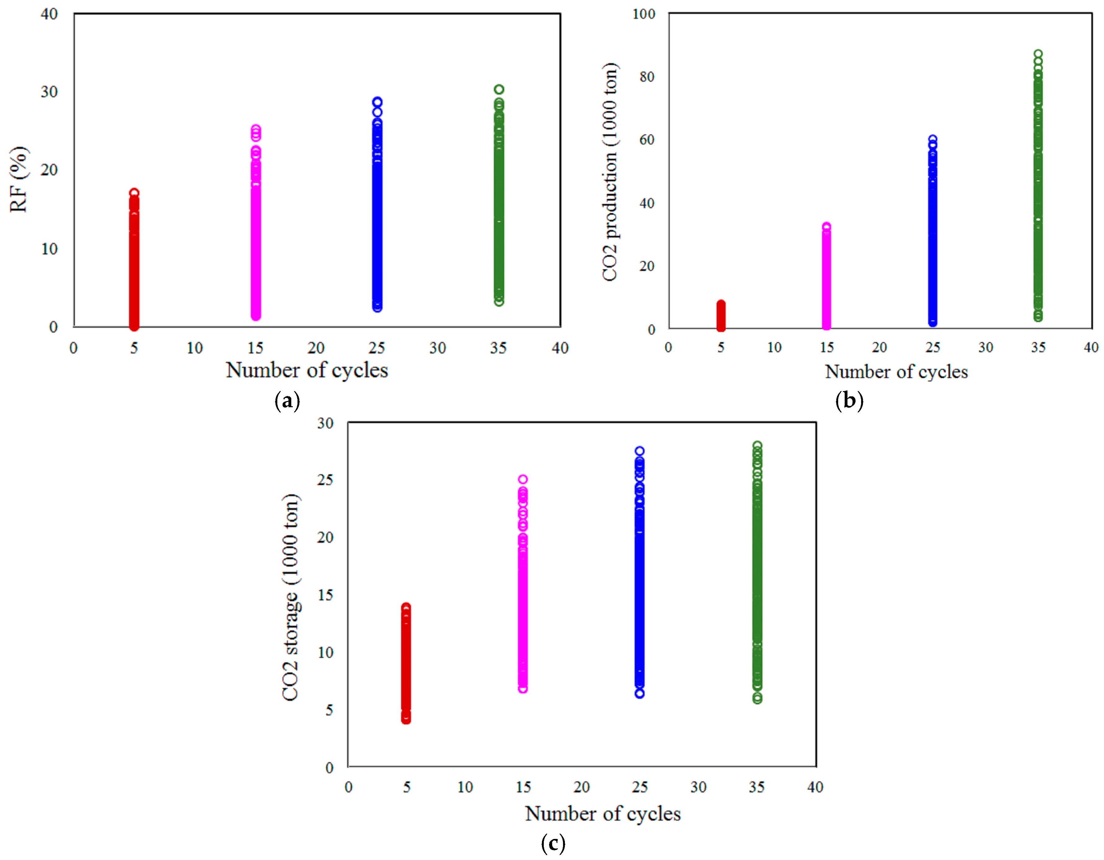
Figure 6.
Training performance for three essential objectives: (a) oil recovery factor; (b) CO2 production; and (c) net CO2 storage.
Figure 6.
Training performance for three essential objectives: (a) oil recovery factor; (b) CO2 production; and (c) net CO2 storage.

Figure 7.
Regression plots for three critical objectives: (a) oil recovery factor; (b) cumulative CO2 production; and (c) net CO2 storage.
Figure 7.
Regression plots for three critical objectives: (a) oil recovery factor; (b) cumulative CO2 production; and (c) net CO2 storage.
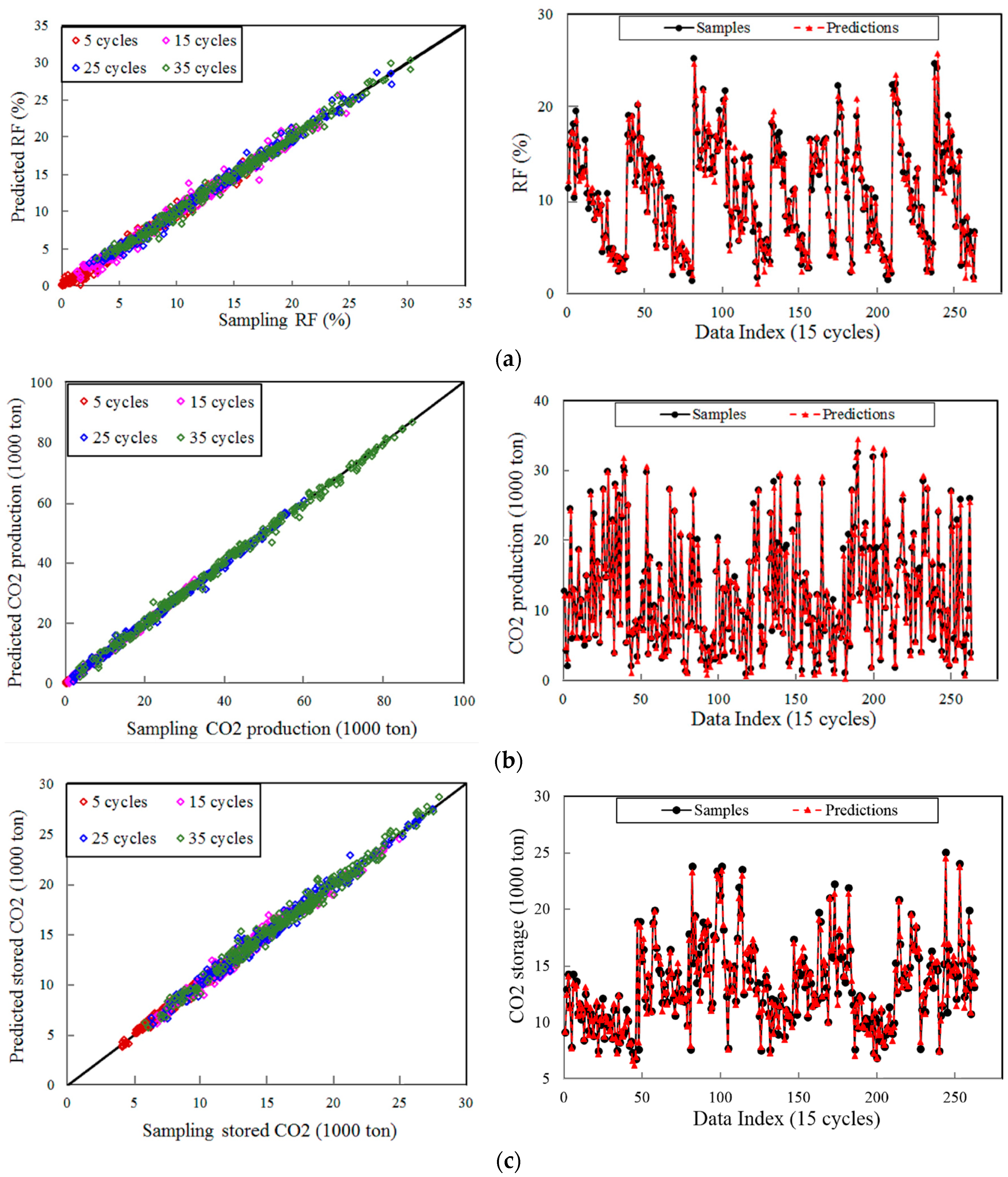
Figure 8.
Relationships between reservoir parameters and flooding performances: (a) Sw and Kv/Kh versus RF; (b) Sw and Kv/Kh versus net CO2 storage.
Figure 8.
Relationships between reservoir parameters and flooding performances: (a) Sw and Kv/Kh versus RF; (b) Sw and Kv/Kh versus net CO2 storage.
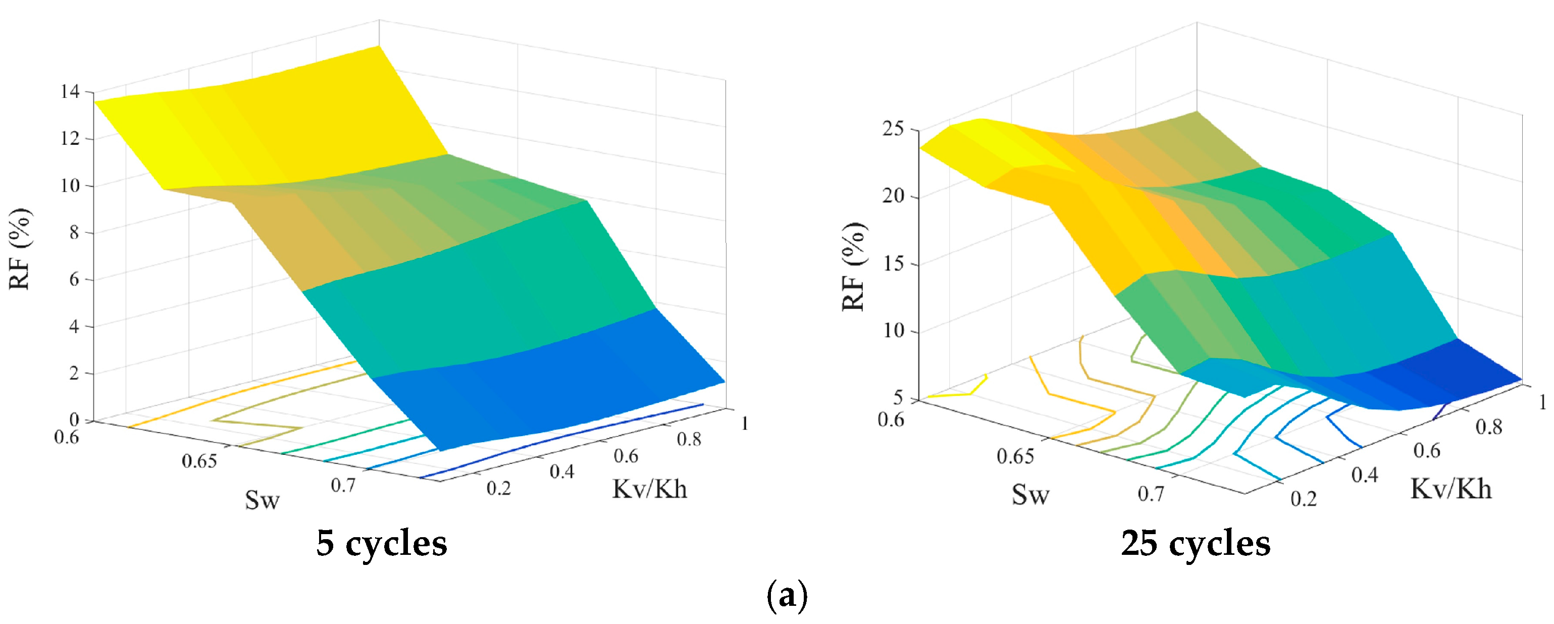

Figure 9.
Dependence of critical targets on the WAG ratio and duration of cycle (T) after 15 and 35 injection cycles: (a) oil recovery; (b) net CO2 storage; and (c) cumulative CO2 production.
Figure 9.
Dependence of critical targets on the WAG ratio and duration of cycle (T) after 15 and 35 injection cycles: (a) oil recovery; (b) net CO2 storage; and (c) cumulative CO2 production.

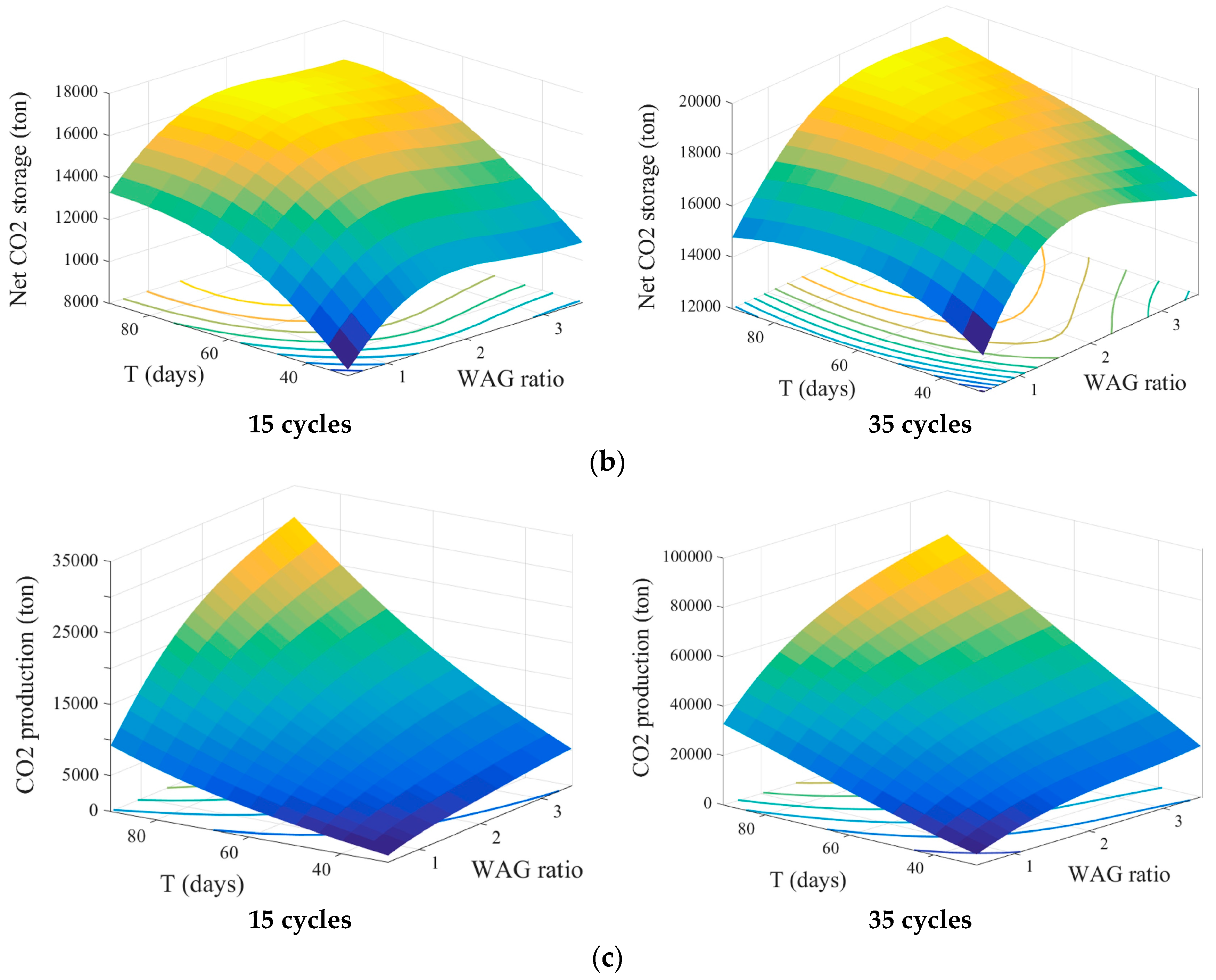
Figure 10.
Dependence effects of the well distance and WAG ratio on targets after 35 cycles: (a) oil recovery factor; (b) cumulative CO2 production; and (c) total CO2 sequestration.
Figure 10.
Dependence effects of the well distance and WAG ratio on targets after 35 cycles: (a) oil recovery factor; (b) cumulative CO2 production; and (c) total CO2 sequestration.
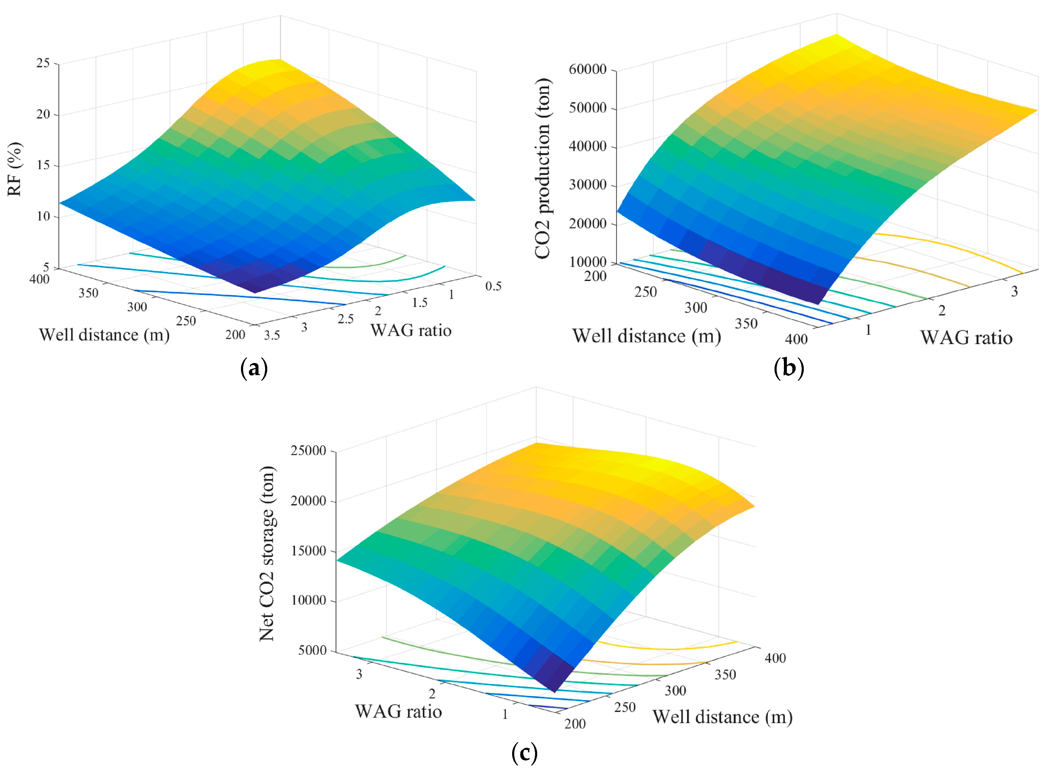
Figure 11.
NPV for six reservoir cases at different oil prices from 35 $/bbl to 65 $/bbl: (a) Sw = 0.6; (b) Sw = 0.7.
Figure 11.
NPV for six reservoir cases at different oil prices from 35 $/bbl to 65 $/bbl: (a) Sw = 0.6; (b) Sw = 0.7.


Table 1.
Reservoir Parameters of the reservoir model at initial conditions.
| Properties | Values | |
|---|---|---|
| Grid size (m3) | 565.84 × 565.84 × 9.15 | |
| Cell size (m3) | 10.48 × 10.48 × 1.52 | |
| Porosity | 0.029–0.21 | |
| Absolute permeability | -Kh (mD) | 10–100 |
| -Kv/Kh (base case) | 0.5 | |
| Reservoir pressure (at bottom layer) (MPa) | 31.026 | |
| Reservoir temperature (°C) | 58.75 | |
| Water saturation (base case) | 0.63 | |
Table 2.
Pseudo-components and parameters of the crude oil used for simulation.
| Components | Mole Fraction | Molecular Weight (g/gmol) | Acentric Factors | Pc (MPa) | Tc (K) |
|---|---|---|---|---|---|
| CO2 | 0.0824 | 44.01 | 0.225 | 7.378 | 304.2 |
| N2 to CH4 | 0.5166 | 16.12 | 0.008229 | 4.59 | 190.11 |
| C2H6 | 0.0707 | 30.07 | 0.098 | 4.89 | 305.4 |
| C3H8 | 0.0487 | 44.10 | 0.152 | 4.25 | 369.8 |
| IC4 to NC5 | 0.0414 | 63.04 | 0.206198 | 3.62 | 436.27 |
| C6 to C9 | 0.0656 | 104.24 | 0.337594 | 2.63 | 523.36 |
| C10 to C14 | 0.0613 | 158.65 | 0.513651 | 2.6 | 659.97 |
| C15 to C19 | 0.0371 | 232.97 | 0.715302 | 1.34 | 855.21 |
| C20+ | 0.0762 | 536 | 1.169989 | 0.852 | 885.57 |
Table 3.
Coefficients of determination and root mean square errors (RMSE) of estimated values from ANN models versus sample data for crucial targets.
Table 3.
Coefficients of determination and root mean square errors (RMSE) of estimated values from ANN models versus sample data for crucial targets.
| Cycles | RF | Gaseous CO2 Production | |||||||
| 5 | 15 | 25 | 35 | 5 | 15 | 25 | 35 | ||
| Training | R2 | 0.990 | 0.991 | 0.996 | 0.994 | 0.989 | 0.996 | 0.998 | 0.998 |
| RMSE (%) | 2.52 | 2.14 | 1.51 | 1.74 | 2.33 | 1.51 | 0.93 | 1.12 | |
| Validation | R2 | 0.981 | 0.978 | 0.990 | 0.990 | 0.978 | 0.995 | 0.997 | 0.996 |
| RMSE (%) | 3.21 | 3.33 | 2.28 | 2.24 | 3.04 | 1.77 | 1.37 | 1.54 | |
| Test | R2 | 0.980 | 0.986 | 0.989 | 0.989 | 0.986 | 0.994 | 0.995 | 0.995 |
| RMSE (%) | 3.82 | 2.89 | 2.47 | 2.61 | 2.87 | 2.09 | 1.74 | 1.72 | |
| Overall | R2 | 0.985 | 0.987 | 0.992 | 0.991 | 0.986 | 0.995 | 0.997 | 0.997 |
| RMSE (%) | 3.10 | 2.65 | 2.0 | 2.14 | 2.66 | 1.75 | 1.31 | 1.42 | |
| Cycles | Net CO2 Storage | ||||||||
| 5 | 15 | 25 | 35 | ||||||
| Training | R2 | 0.988 | 0.986 | 0.993 | 0.991 | ||||
| RMSE (%) | 2.40 | 2.50 | 1.92 | 2.19 | |||||
| Validation | R2 | 0.963 | 0.972 | 0.983 | 0.983 | ||||
| RMSE (%) | 3.57 | 2.99 | 2.45 | 2.50 | |||||
| Test | R2 | 0.980 | 0.976 | 0.982 | 0.978 | ||||
| RMSE (%) | 3.15 | 3.09 | 2.62 | 3.00 | |||||
| Overall | R2 | 0.982 | 0.981 | 0.988 | 0.986 | ||||
| RMSE (%) | 2.90 | 2.79 | 2.26 | 2.52 | |||||
Table 4.
Weights and biases of the ANN structure for RF and Net CO2 storage.
| RF | ||||||||||
| b | IW | LW | ||||||||
| b1 | b2 | D | Sw | Kv/Kh | WAG | T | 5 | 15 | 25 | 35 |
| 0.120 | −0.586 | −0.207 | −1.673 | −0.280 | −0.394 | 1.388 | 0.162 | 0.027 | 0.017 | 0.017 |
| −3.651 | −1.514 | 0.213 | 2.523 | −0.113 | −0.135 | 0.030 | −0.639 | 0.381 | 0.700 | 0.895 |
| −1.824 | −1.000 | 0.339 | 0.049 | −0.351 | −0.109 | −0.625 | 0.014 | −1.920 | −1.575 | −1.234 |
| −0.960 | −0.556 | 0.680 | −0.337 | −0.753 | −0.793 | −1.100 | −0.132 | 0.096 | 0.097 | 0.085 |
| 0.177 | - | 0.475 | −1.441 | −0.189 | −0.489 | 0.175 | 0.152 | 0.313 | 0.324 | 0.330 |
| −2.821 | - | 0.156 | −2.591 | −0.056 | −0.815 | 0.590 | 0.553 | 0.265 | 0.216 | 0.203 |
| 1.413 | - | −0.010 | 0.089 | 1.570 | 0.388 | −0.078 | −0.273 | −1.235 | −1.553 | −1.675 |
| −0.963 | - | −0.146 | 2.437 | −0.374 | −1.161 | −0.001 | −0.963 | −0.822 | −0.854 | −0.906 |
| −1.787 | - | −0.226 | −0.119 | −1.654 | −0.444 | 0.123 | −0.189 | −1.126 | −1.500 | −1.668 |
| −0.721 | - | −0.114 | 2.403 | −0.350 | −1.512 | −0.011 | 0.931 | 0.728 | 0.735 | 0.771 |
| CO2 Production | ||||||||||
| b | IW | LW | ||||||||
| b1 | b2 | D | Sw | Kv/Kh | WAG | T | 5 | 15 | 25 | 35 |
| 2.210 | −0.418 | −0.273 | 0.033 | −1.923 | −0.269 | −0.336 | 0.357 | 0.529 | 0.397 | 0.340 |
| 0.314 | −0.653 | −0.275 | 0.065 | 0.282 | 0.460 | 0.525 | −1.999 | 0.277 | 0.793 | 0.947 |
| 0.142 | −0.867 | −0.523 | 0.164 | 0.447 | 1.466 | 0.644 | 0.375 | 0.063 | −0.078 | −0.135 |
| 1.204 | −0.949 | −0.295 | 0.051 | −0.676 | −0.363 | −0.516 | −0.522 | −0.935 | −0.727 | −0.623 |
| −0.174 | - | 0.370 | 0.018 | −0.568 | −0.076 | −0.419 | −0.852 | −0.002 | 0.260 | 0.375 |
| −0.768 | - | −0.133 | 0.074 | −0.046 | 0.518 | −0.413 | 0.055 | −0.398 | −0.459 | −0.474 |
| −1.388 | - | −0.712 | −0.077 | −0.690 | −0.226 | 0.706 | 0.111 | 0.330 | 0.275 | 0.208 |
| −1.780 | - | −0.195 | 0.054 | 0.066 | −1.009 | 0.521 | −1.014 | −1.029 | −1.031 | −1.025 |
| 0.415 | - | −0.065 | −0.105 | 0.105 | 0.470 | 0.780 | 0.827 | 0.065 | 0.078 | 0.135 |
| −0.866 | - | −0.517 | 0.135 | 0.186 | 0.185 | 0.737 | 1.006 | 0.565 | 0.426 | 0.406 |
| Net CO2 Storage | ||||||||||
| b | IW | LW | ||||||||
| b1 | b2 | D | Sw | Kv/Kh | WAG | T | 5 | 15 | 25 | 35 |
| −3.181 | −1.218 | 0.894 | 0.058 | −2.133 | 0.758 | −0.060 | 0.034 | 0.312 | 0.356 | 0.308 |
| −1.130 | −1.758 | 0.543 | −0.039 | −0.051 | −0.383 | −0.411 | −0.071 | −1.229 | −1.588 | −1.487 |
| −0.763 | −1.575 | 0.359 | −0.107 | −0.167 | −0.725 | −0.552 | −1.317 | 0.096 | 0.690 | 0.733 |
| −0.202 | −1.365 | 1.240 | 0.055 | 1.116 | 0.447 | −0.708 | −0.067 | −0.207 | −0.120 | −0.029 |
| −0.081 | - | 0.234 | −0.187 | −0.496 | −0.389 | 0.102 | 0.422 | 0.319 | 0.429 | 0.547 |
| 0.120 | - | 0.520 | −0.024 | 0.153 | 0.112 | 0.527 | 0.362 | 0.656 | 0.487 | 0.293 |
| 0.069 | - | 0.159 | −0.042 | −0.089 | −1.081 | 0.032 | 0.784 | 0.403 | 0.169 | 0.117 |
| −0.905 | - | −0.429 | −0.061 | −0.249 | −0.711 | 0.079 | −0.294 | −0.887 | −1.221 | −1.366 |
| 1.142 | - | 0.039 | −0.042 | −0.072 | −0.948 | −1.268 | −0.463 | 0.050 | 0.137 | 0.078 |
| 0.592 | - | 0.163 | −0.092 | −0.126 | 0.349 | −0.718 | 0.903 | 0.577 | 0.184 | 0.046 |
Table 5.
Specific fiscal conditions for a WAG flooding project.
| Components | Values |
|---|---|
| Oil price | 35–65 ($/bbl) |
| CO2 purchase cost | 17.5 ($/ton) |
| CO2 recycling cost | 12 ($/ton) |
| CO2 gathering system | 30,000 ($/pattern) |
| Operating costs | 60,000 ($/year/pattern) |
| Additional incentives | 3.5 ($/ton CO2 storage) |
| Discount rate | 12% |
| Income tax | 35% |
Table 6.
Optimal injection designs and well distances for different Sw and Kv/Kh values in terms of NPV (oil price at 45 $/bbl).
Table 6.
Optimal injection designs and well distances for different Sw and Kv/Kh values in terms of NPV (oil price at 45 $/bbl).
| Sw = 0.6 | Kv/Kh = 0.1 | Kv/Kh = 0.5 | Kv/Kh = 1 |
|---|---|---|---|
| 25 Cycles | 25 Cycles | 25 Cycles | |
| RF (%) | 25.18 | 19.40 | 17.67 |
| NPV ($MM) | 1.993 | 1.846 | 1.665 |
| D (m) | 400 | 280 | 300 |
| WAG | 0.5 | 0.5 | 0.5 |
| T (days) | 50 | 30 | 30 |
| Sw = 0.7 | Kv/Kh = 0.1 | Kv/Kh = 0.5 | Kv/Kh = 1 |
| 25 Cycles | 25 Cycles | 25 Cycles | |
| RF (%) | 17.43 | 11.94 | 7.89 |
| NPV ($MM) | 0.834 | 0.546 | 0.387 |
| D (m) | 400 | 400 | 400 |
| WAG | 0.5 | 0.5 | 0.5 |
| T (days) | 60 | 55 | 40 |
© 2017 by the authors. Licensee MDPI, Basel, Switzerland. This article is an open access article distributed under the terms and conditions of the Creative Commons Attribution (CC BY) license (http://creativecommons.org/licenses/by/4.0/).
Share and Cite
MDPI and ACS Style
Le Van, S.; Chon, B.H. Applicability of an Artificial Neural Network for Predicting Water-Alternating-CO2 Performance. Energies 2017, 10, 842. https://doi.org/10.3390/en10070842
AMA Style
Le Van S, Chon BH. Applicability of an Artificial Neural Network for Predicting Water-Alternating-CO2 Performance. Energies. 2017; 10(7):842. https://doi.org/10.3390/en10070842
Chicago/Turabian StyleLe Van, Si, and Bo Hyun Chon. 2017. "Applicability of an Artificial Neural Network for Predicting Water-Alternating-CO2 Performance" Energies 10, no. 7: 842. https://doi.org/10.3390/en10070842
Note that from the first issue of 2016, this journal uses article numbers instead of page numbers. See further details here.